DFT+DMFT with natural atomic orbital projectors

Abstract

We introduce natural atomic orbitals as the local projector to define the correlated subspace for DFT + DMFT (density functional theory plus dynamical mean-field theory) calculation. The natural atomic orbitals are found to be stably constructed against the number and the radius of basis orbitals. It can also be self-consistently updated inside the DFT+DMFT loop. The spatial localization, electron occupation and the degree of correlation are investigated and compared with other conventional techniques. As a ‘natural’ choice to describe the electron numbers, adopting natural atomic orbitals has advantage in terms of electron number counting. We further explore the reduction of computation cost by separating correlated orbitals into two subgroups based on the orbital occupancy. Our new recipe can serve as a useful choice for DFT+DMFT and related methods.

I Introduction

The calculation of real materials with strong electronic correlations poses an important problem in condensed matter physics and material science. While the first-principles band structure method based on density functional theory (DFT) provides a powerful theoretical framework for real materials, the sizable on-site correlation invalidates the standard approximations such as local density approximation (LDA) and generalized gradient approximation (GGA). To overcome this limitation, the combined methods of LDA/GGA with many-body techniques have been suggested and made tremendous success such as the early attempts of so-called LDA$+U$ or DFT$+U$ Anisimov et al. (1991, 1993) and the more recently suggested LDA+Gutzwiller Ho et al. (2008); Gutzwiller (1965); Deng et al. (2009); Lanatà et al. (2015). GW type of self energy within the self-consistent framework van Schilfgaarde et al. (2006); Kotani et al. (2007); Faleev et al. (2004) can also be useful with the limited purposes of, e.g., describing the model parameters and the metallic Fermi surfaces Jang et al. (2015); Ryee et al. (2016). Among them, DFT+DMFT (dynamical mean-field theory) has become one of the standard choices providing the unique feature by capturing the ‘dynamic’ correlations Georges and Kotliar (1992); Metzner and Vollhardt (1989); Zhang et al. (1993); Anisimov et al. (1997); Lichtenstein and Katsnelson (1998); Kotliar et al. (2006); Georges et al. (1996).

Along with its great success, many of formal and technical issues in the implementation have received much attention Amadon et al. (2008); Anisimov et al. (2005); Savrasov et al. (2001); Held et al. (2001a, b); Park et al. (2008); de’ Medici et al. (2011); Kent and Kotliar (2018); Choi et al. (2019); _DM ; Alet et al. (2005); Parcollet et al. (2015); Haule et al. (2010). Typically, any attempt to combine LDA/GGA-type of scheme with Hubbard-like model approach requires a step to define the correlated subspace within which Coulomb interaction (‘Hubbard $U$’) comes in to play. In other words, the correlated orbitals span the bands near the Fermi level ($E_{F}$) where the on-site correlation becomes important. They are expected to be reasonably well localized, site-centered and atomic-like. In literature, many different suggestions to define the correlated orbital space are found: maximally localized Wannier functions (MLWF) Souza et al. (2001); Marzari and Vanderbilt (1997), muffin-tin orbitals Andersen and Saha-Dasgupta (2000); Pavarini et al. (2004), and other projection methods Haule et al. (2010, 2014).

Considering the ambiguity in this choice of ‘projector’, we take a special note of recent studies that emphasize the correlated orbital occupancy $N_{d}$ being the critical variable to describe the correlation effect Wang et al. (2012); Dang et al. (2014). Here it should first be noted that estimating or determining $N_{d}$ is a non-trivial issue. It depends on the form of so-called double counting form Wang et al. (2012); Dang et al. (2014) as well as the choice of the correlated orbitals Haule et al. (2014). In fact, it is not straightforward already in DFT-LDA level, leading to many different possible choices suggested for atomic orbitals or charge counting schemes such as Mulliken population analysis Mulliken (1955a, b), Löwdin orthogonalization method Löwdin (1950) and natural population analysis Reed et al. (1985).

In this paper we suggest the implementation of DFT+DMFT with natural atomic orbitals (NAOs) as the local projector. In our DFT formulation based on the linear combination of non-orthogonal pseudo-atomic orbitals (PAOs) ope , the use of NAOs provides a ‘natural’ way of estimating $N_{d}$ from the orthogonalized orbitals. The NAO construction process is not only well plugged in between DFT and DMFT self-consistent loop, but it also stable with respect to the numerical parameters such as the range of energy window and the number of basis sets. Our calculations show that the localization and the covalency are reasonably well described with NAO compared with the other choices including PAO, L${\rm\ddot{o}}$wdin orthogonalized orbital (LOO), and MLWF. Further, the possibility of reducing computation cost is explored by separating the correlated subspace into two different parts.

The paper is organized as follow. In Sec. II we briefly review the DFT+DMFT procedure which is followed by our NAO-based formalism. In Sec. III, the calculation results are presented for a correlated metal SrVO₃ and a charge-transfer insulator NiO. Summary and conclusion are given in Sec. IV.

II Formalism

II.1 DFT+DMFT and the basis issue

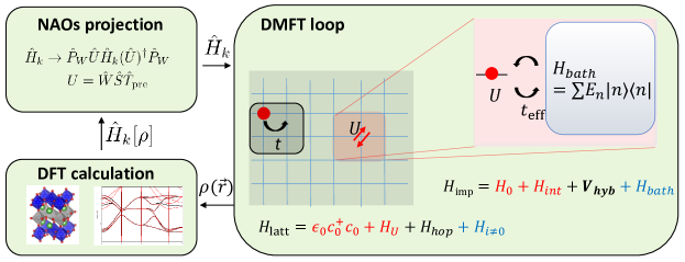
Figure 1: A schematic illustration of our DFT+DMFT calculation by using NAO as local projector. Kohn-Sham DFT Hamiltonian is solved within LDA or GGA which provides the charge density and overlap matrix. With those, one can construct NAOs which then serve as correlated orbitals for DMFT impurity model. As in the conventional DFT+DMFT, Kohn-Sham Hamiltonian $H_{k}$ obtained from LDA/GGA is regarded as non-interacting $H_{0}$ for DMFT calculation. The computed Green’s function $G_{{\rm imp}}$ and the self-energy $\Sigma_{{\rm imp}}$ complete the self-consistent loop by providing the updated charge density $\rho(\vec{r})$ for DFT-LDA/GGA.

So-called DFT+DMFT is a scheme that combines the standard band theory such as LDA and GGA with a non-perturbative many-body technique, DMFT. In DMFT, the lattice self-energy $\hat{\Sigma}_{{\rm latt}}(i\omega_{n},\bm{k})$ is approximated by local self-energy $\hat{\Sigma}^{\rm DMFT}_{{\rm latt}}(i\omega_{n})=\bigoplus_{R}\ \hat{\Sigma}_{{\rm loc}}(R)$. The non-local contribution is projected out by a local projection; $\hat{\Sigma}_{\rm loc}(R)=P_{R}\hat{\Sigma}_{{\rm latt}}=\sum_{\alpha\beta\in d}\ket{\chi_{\alpha R}}\Sigma_{\alpha\beta}(R)\bra{\chi_{\beta R}}$ where ‘$d$’ refers to the correlated subspace such as transition-metal $d$ orbitals and $R$ the atomic position. The on-site Coulomb interaction is applied onto the localized orbitals $\ket{\chi_{\alpha}}$. The interacting Green’s function is given by

$$\hat{G}(i\omega_{n},\bm{k})=\frac{{1}}{i\omega_{n}+\mu-\hat{H}(\bm{k)}-\hat{\Sigma}_{{\rm loc}}(i\omega_{n})+\hat{\Sigma}_{dc}(i\omega_{n})}$$ (1)

where $\hat{\Sigma}_{dc}$ refers to the double-counting term. Once $P_{R}$, or correlated subspace $\{\ket{\chi_{\alpha}}\}$ is specified, $\hat{\Sigma}_{{\rm loc}}$ is determined by solving the impurity model with the self-consistently-constructed hybridization function Zhang et al. (1993); Lichtenstein and Katsnelson (1998); Georges and Kotliar (1992); Metzner and Vollhardt (1989):

$$\hat{\Delta}(i\omega_{n})=P_{R=0}\left[i\omega_{n}-\hat{H}_{{\rm loc}}-\Sigma_{{\rm loc}}(i\omega_{n})+\Sigma_{{\rm dc}}(i\omega_{n})-\left(\frac{1}{N_{k}}\sum_{k}\hat{G}(\bm{k},i\omega_{n})\right)^{-1}\right].$$ (2)

Many issues can arise in solving this problem. The first thing is to choose ‘impurity solver’ for which several standard techniques are available such as (continuous-time) quantum Monte Carlo ((CT)QMC) Werner et al. (2006); Werner and Millis (2006), exact diagonalization Koch et al. (2008); Caffarel and Krauth (1994), NRG (numerical renormalization group) Wilson (1975); Bulla et al. (2008) and others Bauernfeind et al. (2017), each of which has both advantage and disadvantage. Another important issue is related to $\hat{\Sigma}_{dc}(i\omega_{n})$ for which many different recipes have been discussed in literature Wang et al. (2012); Karolak et al. (2010); Haule (2015, 2015); Anisimov et al. (1991, 1993) In the current study, we take so-called ‘fully localized limit’ as suggested in Ref. Anisimov et al., 1993.

Our main concern here is about the projection for defining the correlated subspace $\left\{\ket{\chi_{\alpha}}\right\}$ in the line of previous discussion Wang et al. (2012); Haule et al. (2014); Dang et al. (2014). Note that different projection method can lead to the different self-energy. Several different ways to construct localized orbitals have been suggested. For example, maximally localized Wannier function (MLWF) method is widely used in combination with different type of codes Lechermann et al. (2006); Bhandary et al. (2016); _DC . One can also take LMTO (linearized muffin-tin orbitals) L. V. Pourovskii et al. (2007), NMTO (n-th order muffin-tin orbitals) Lechermann et al. (2006), or resort to the real space embedding method Haule et al. (2010).

As an alternative possible choice, we pay a special attention to ‘projective Wannier function (PWF)’ method which is a straightforward way to define correlated orbitals Amadon (2012); Amadon et al. (2008). It has been adopted in some standard computation schemes including LMTO Anisimov et al. (2005), APW Aichhorn et al. (2009); Karolak et al. (2011); Schüler et al. (2018), and PAW Amadon (2012); Amadon et al. (2008). The main idea of PWF is to project the localized atomic-like orbitals $\left\{\ket{\tilde{\chi}_{\alpha}}\right\}$ onto the the low-energy Bloch states

$$\ket{\chi_{\alpha}}=\frac{{1}}{N}\sum_{k,n}^{\epsilon_{kn}\in W}\ket{kn}\braket{kn}{\tilde{\chi}_{\alpha}},$$

followed by orthogonalization procedure Amadon et al. (2008). Here $N=\lVert\sum_{k,n}^{\epsilon_{kn}\in W}\ket{kn}\braket{kn}{\tilde{\chi}_{\alpha}}\rVert$ is the normalization factor and $W$ energy window within which the hybridization function $\Delta(i\omega_{n})$ is defined. Thus the result depends not only on the energy window $W$ but also on the choice of initial local orbitals $\left\{\ket{\tilde{\chi}_{\alpha}}\right\}$. While the ambiguity related to the $W$ range can be removed, at least in principle by taking the large enough energy window Haule et al. (2014), the choice of the $\ket{\tilde{\chi}_{\alpha}}$ is not straightforward. The different initial choice can lead to the different final result Karolak et al. (2011).

A purpose of our current work is to construct the optimal $\ket{\tilde{\chi}_{\alpha}}$ for the non-orthogonal local orbital basis method. As mentioned above, the result of DFT+DMFT can critically depend on the choice of $\ket{\tilde{\chi}_{\alpha}}$. Non-orthogonality can introduce an ambiguity in the estimation of key physical quantities such as the number of electrons in $d$ orbitals $N_{d}$. This poses a highly non-trivial issue not only because the correlated orbitals often get significantly hybridized with ligands but also because the numerical orthogonalization process usually introduces the undesirable mixing between the two. Here we suggest NAOs Reed et al. (1985) as a set of the local correlated orbitals $\ket{\tilde{\chi}_{\alpha}}$ for DFT+DMFT calculation. As illustrated in Fig. 1, this process can be inserted as an intermediate step between DFT and DMFT to complete the self-consistent loop. While ‘natural orbital’ has been adopted for the basis set to solve the impurity model Kananenka et al. (2015), we emphasize that the use of $\ket{\chi_{\alpha}^{{\rm NAOs}}}$ as $\ket{\tilde{\chi}_{\alpha}}$ has never been reported for the first-principles DFT+DMFT.

The use of NAO as a local projector has notable advantages. As will be discussed in the below, this choice can certainly give the more intuitive charge counting for the correlated orbitals. Further, the construction of NAOs is found to be numerically stable. In the case of MLWF, for example, achieving the convergence can be an issue when the bands are strongly entangled. As for muffin-tin orbitals or PAOs, basically the similar ambiguity can be manifested in terms of the choice of local orbital radius. In this sense, the use of NAO can be a ‘natural’ choice regardless of the DFT basis types.

II.2 Natural atomic orbital as a projector

The numerical PAOs basis in our DFT code, OpenMX, is constructed in a controlled way and therefore its localization is well identified Ozaki and Kino (2004); Ozaki (2003). The non-orthogonality issue, on the other hand, needs to be dealt with care. One straightforward way is just to take $\ket{\tilde{\chi}_{\alpha}}=\ket{\phi^{{\rm PAOs}}}$ as correlated orbitals and to reconstruct the ligand orbitals to be orthogonal with respect to $\ket{\tilde{\chi}_{\alpha}}$ through, e.g., Schmidt orthogonalization procedure. This choice corresponds to ‘full’ local projector in the previous DFT$+U$ implementation Han et al. (2006). Not surprisingly, however, this procedure overestimates the electron occupation in the correlated orbitals as discussed in the below (see Sec. III). Another possible choice, namely, Löwdin symmetric orthogonalization, is not the desirable method either because it treats the important atomic set (the AO with large occupations) and the less important AO (the almost empty AO) on the equal footing.

Here we note that NAOs can be determined in a physically motivated way and suitable for local orbitals of the given materials Reed et al. (1985). Mathematically, NAOs are defined by the eigen-orbitals of any given local occupation matrix Löwdin (1955). For a given occupation matrix $N^{\rm PAOs}_{\alpha\beta}=\braket{c_{\alpha}^{\dagger}c_{\beta}}$ NAOs are constructed through a three-step process. In the below, orbital index $\alpha\equiv(ilp)$ specifies the site index $i$, angular momentum quantum number $l$, and multiplicity number of radial basis function $p$. First, we construct the atom-centered local orbitals $\ket{\phi^{{\rm pre}}}$ called as ‘pre-NAOs’ which are the eigenstates of the sub-block $(N^{i,l})_{pp^{\prime}}$ corresponding to the occupation matrix projected onto the atomic site $i$ and the angular momentum $l$ subshells. To preserve the invariance of the occupation with respect to the coordinate transformation, the symmetry averaging should be carried out over the $(2l+1)$ diagonal blocks of $N_{pp^{\prime}}^{i,l}$. Since the pre-NAO transformation matrix $\hat{T}_{\rm pre}^{i,l}$ considers only the sub-blocks of the occupation matrix, pre-NAOs centered on different atoms are nonorthogonal to one another.

The second and third step concern about the proper elimination of inter-atomic wave function overlaps. To obtain a stable result, we divide pre-NAOs into two subsets, namely, ‘minimal’ and ‘Rydberg’ set Reed et al. (1985). The ‘minimal’ set is the atomic $(n,l)$ subshells with finite formal occupancy whereas the ‘Rydberg’ set consists of the remaining (formally unoccupied) orbitals. Then the ‘Rydberg’ sets are Schmidt orthogonalized to the manifold spanned by ‘minimal’ orbitals. We represent this orthogonalization by a matrix $\hat{S}$. This step is essential to avoid the over-counting problem in the occupancy-weighted symmetric orthogonalization (OWSO) process in the next step.

In the third step, we orthogonalize pre-NAOs orbitals by means of OWSO method in which the occupancy-weighted difference between orthogonalized basis and original pre-NAOs

$$\sum_{\alpha}N_{\alpha\alpha}\lVert\ket{\chi_{\alpha}^{{\rm NAOs}}}-\ket{\phi_{\alpha}^{{\rm pre}}}\rVert^{2}$$ (3)

is minimized. Here, $N$ is expressed within pre-NAOs basis. The transformation having this property is written as

$$\ket{\chi_{\alpha}^{{\rm NAOs}}}=\ket{\phi_{\beta}^{PAOs}}W_{\beta\alpha},$$ (4)

where $\hat{W}=\tilde{N}(\tilde{N}O\tilde{N})^{-1/2}$ with the overlap matrix of pre-NAOs ($O$), and the diagonal part of $N$ ($\tilde{N}$). The final form of transformation matrix from PAOs to NAOs can then be written as $\hat{T}_{N}=\hat{W}\hat{S}\hat{T}_{Pre}$.

Natural orbital methods, including NAO and natural bond orbital, have been used typically to calculate atomic charge population Reed et al. (1985, 1988). Recently, natural orbitals have also been used to solve impurity problem of strongly correlated electron systems Go and Millis (2017); Mayda et al. (2017). For example, natural orbitals can provide the adaptive basis set to reduce the dimension of Hilbert space Go and Millis (2017). In Ref. Mayda et al., 2017, model parameters for Anderson impurity problem have been obtained based on NAOs. In the current study, we used NAO as a basis or a projector for representing correlated subspace. We also demonstrate that the use of NAO can provide a way of reducing computation costs by separating the correlated orbitals into two subsets and adopting two different levels of solvers as will be discussed in the below.

III Application

III.1 Computation details

First-principles band calculations have been carried out based on DFT within LDA Perdew and Zunger (1981); Ceperley and Alder (1980). We used ‘OpenMX’ code ope ; Ozaki and Kino (2004); Ozaki (2003) for DFT calculation. Experimental lattice parameters have been used Rey et al. (1990); Furstenau et al. (1985), and the $k$-point meshes of $13\times 13\times 13$ and $23\times 23\times 23$ adopted for SrVO₃ and NiO, respectively. Double valence and single polarization orbitals were used as a basis set for DFT. These numerical atomic basis orbitals (i.e., PAOs) were generated with cutoff radius of 10.0, 6.0, 6.0, and 5.0 a.u. for Sr V, Ni, and O atoms, respectively Ozaki and Kino (2004). The DFT-LDA calculation results serve as the non-interacting Hamiltonian $H_{0}$, and the interaction Hamiltonian containing the density-density interaction is parameterized by $U$ and $J_{H}$ for on-site Coulomb repulsion and Hund interaction, respectively. The Hamiltonian is solved within the single-site DMFT by employing hybridization expansion CT-QMC algorithm Gull et al. (2001, 2011). For ‘impurity solver’, we used the software package as implemented in Ref. Haule, 2007; _CT, , and the results were double checked by using ALPS library Alet et al. (2005). Our DFT+DMFT interface code is available online _DM . The real frequency self-energy and spectral function are obtained from the matsubara Green’s function and the self-energy by analytic continuation using maximum entropy method (MEM) Jarrell and Gubernatis (1996); Gunnarsson et al. (2010). For this process we used our recent method as reported in Ref. Sim and Han, 2018. The large enough energy windows of $W=[-10,10]$ eV around $E_{F}$ has been considered Rey et al. (1990); Haule et al. (2014). For comparison, we also present the results of MLWF as local projectors where the initial projections onto three atomic V-$t_{2g}$ and nine O-$2p$ orbitals were used for SrVO₃ Souza et al. (2001); Marzari and Vanderbilt (1997).

III.2 SrVO₃

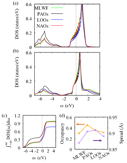
Figure 2: (a) The calculated density of states projected onto the V-$t_{2g}$-like orbitals for SrVO₃ with $U=0$ eV. The results from the different local orbitals, namely MLWF (green), PAOs (black), LOOs (blue), and NAOs (red), are compared. (b) The calculated spectral function $A(\omega)$ projected onto the local orbitals with $U$ = 6 eV and at inverse temperature $\beta=20$ eV^-1. (c) The integrated density of states for different local orbitals. (d) The calculated occupancy of each $t_{2g}$ orbitals within LDA+DMFT calculation (orange) and the spread of the orbitals as defined in the text (purple).

SrVO₃ has been serving as a test bed for DFT+DMFT Nekrasov et al. (2005, 2006); Karolak et al. (2011); Sekiyama et al. (2004); Nomura et al. (2012) and the related methods such as LDA+DCA Lee et al. (2012) and $GW$+DMFT Taranto et al. (2013); Casula et al. (2012); Tomczak et al. (2014, 2012); Choi et al. (2016). With cubic SrVO₃ as our first example, we investigated the properties of NAO as a local projector. Fig. 2(a) and (b) shows the LDA ($U=0$ eV) and the LDA+DMFT density of states (DOS) projected onto the V-$t_{2g}$ like orbitals, respectively. Two main peaks are clearly identified; the O_p–V_d bonding complex locating at around $[-7{\rm eV},-3{\rm eV}]$, and the the antibonding states across $E_{F}$ which are mainly of V_d character. The results of four different projectors are presented in different colors, namely, the green, black, blue and red lines refer to the MLWF, PAO, LOO, and NAO result, respectively.

Not surprisingly, the degree of hybridization depends on the choice of projectors. For example, the direct use of PAOs notably overestimates $d$-$p$ hybridization compared to the other projection methods. This feature is reflected in that the more states of the lower-lying bonding complex are assigned as V_d orbitals; see Fig. 2(a) and (b). Also, it naturally affects the electron number counting. With PAO projector, $n_{e_{g}}^{\rm LDA}=\sum_{n,k}^{\epsilon_{nk}<\epsilon_{F}}\lvert\braket{nk}{\tilde{\chi}_{\alpha}^{{\rm PAO}}}\rvert^{2}=0.55$ and $n_{t_{2g}}^{\rm LDA}=\sum_{n,k}^{\epsilon_{nk}<\epsilon_{F}}\lvert\braket{nk}{\tilde{\chi}_{\beta}^{{\rm PAO}}}\rvert^{2}=0.50$, where $\alpha\in e_{g}$ and $\beta\in t_{2g}$. Both values of $n_{t_{2g}}^{\rm LDA}$ and $n_{e_{g}}^{\rm LDA}$ are notably larger than those of NAOs; $n_{e_{g}}^{\rm LDA}=0.29$ and $n_{t_{2g}}^{\rm LDA}=0.35$. The nominal values ($t_{2g}^{1}$ configuration of V⁴⁺) are $n_{e_{g}}=0$ and $n_{t_{2g}}=1/6$. Note that $n_{t_{2g}}^{\rm LDA}<n_{e_{g}}^{\rm LDA}$ in PAO projection whereas $n_{t_{2g}}^{\rm LDA}>n_{e_{g}}^{\rm LDA}$ in NAO.

The same feature can also be noted in the integrated DOS (IDOS) as presented in Fig 2(c). The calculated IDOS at $E_{F}$ clearly shows that the V_d occupation or its valency is markedly larger in the PAO estimation than in others. The calculated IDOS at $E=E_{F}$ is 0.34, 0.50, 0.31, and 0.35 for MLWF, PAO, LOO, and NAO, respectively. The largest value of PAO projector reflects the greatest $d$–$p$ hybridization while the value of NAO is smaller than that of PAO and comparable with MLWF. Another notable feature is that the IDOS calculated from LOOs does not reach to but remains far below 1.0 even up to $\omega=+10$ eV; $\simeq$ 0.78. On the other hand, the use of PAO and NAO projector satisfies the sum rule, yielding the IDOS $\simeq$0.96 and 0.97 (i.e., close to 1.0), respectively, as $\omega$ becomes large.

This feature remains stable even when the number of basis orbitals (not the projector orbitals) changes. The calculation with the more basis orbitals of $s2p2d2f$$1$ (i.e., double orbital sets for $s$, $p$, $d$, and single for $f$ states), for example, gives $n_{t_{2g}}^{\rm LDA}=0.31$ by using NAO projector. The calculated IDOS up to high energy remains as 0.97. On the other hand, the IDOS result of LOO, 0.72, shows the sizable dependence on the basis set choice due to the mixing between the correlated orbitals near $E_{F}$ and the atomic orbitals in the higher energy. These features can certainly be useful for both practically and physically.

In order to see and compare the degree of spatial localization of correlated orbitals produced by different projectors, we computed the ‘spread function’ Marzari and Vanderbilt (1997) defined by $\Omega=\sqrt{{\braket{\mathbf{r}^{2}}-\braket{\mathbf{r}}^{2}}}$ where $\braket{\mathbf{r}}=\int\mathbf{r}\lvert\tilde{\chi}_{\alpha\in t_{2g}}(\mathbf{r})\rvert^{2}d\mathbf{r}$  . The results of the energy window $W=[-10,10]$ eV are presented in Fig. 2(d). The calculated $\Omega$ for NAOs is 0.891 Å which is slightly larger than that of MLWF (0.870 Å), and smaller than PAO ($0.905$ Å) and LOO ($0.910$ Å). Our analysis shows that the NAO projector produces a moderately localized spatial subspace of correlation.

The DFT+DMFT result of $A(\omega)=-1/\pi\Im G_{{\rm loc}}(\omega)$ is presented in Fig. 2(b). The calculations were performed with the inverse temperature $\beta=20$ eV^-1, $U=6.5$ eV and $J_{H}=0.65$ eV Amadon et al. (2008). The effect of correlation is clearly seen in the bandwidth renormalization and the upper Hubbard-like peak developed at around $\omega=+2$eV, both of which clearly show that the correlation effect is gradually reduced as the more localized projector is adopted. The use of NAO gives the moderate degree of correlation in between MLWF and PAO. Focusing on the lower and upper Hubbard peak, identified at around $\omega=-1$ and $+2.5$ eV, respectively, they are more pronounced in the result of MLWF than PAO. Once again, the result of NAO is in the middle being consistent with the above analysis. A systematic trend of correlation strength depending on the local projectors is also observed in the calculated spectral weight of the bonding orbital complex.The calculated $A(\omega)$ with PAO projector has the much greater weight in this region of energy reflecting the larger hybridization between V-$t_{2g}$ and O-$p$ states. This is attributed to the extended and non-orthogonal nature of PAO.

Fig. 2(d) also shows the electron occupancy in V${}_{t_{2g}}$ orbitals, $n_{t2g}^{\rm DMFT}$, obtained from LDA+DMFT calculation with different local projectors. The NAO shows the comparable value with that of MLWF which is noticeably smaller than the other projection results. The use of more localized projector results in the smaller occupation which is consistent with the previous studies on covalency issue Wang et al. (2012); Dang et al. (2014); Haule et al. (2014).

A straightforward and quantitative way to measure the correlation effect is to estimate the quasi-particle renormalization factor

$$Z\approx\left[1-\frac{\Im\Sigma(i\omega_{1})}{\omega_{1}}\right]^{-1}.$$ (5)

The calculated value by NAO projector is $Z^{\rm NAO}=0.60$ which is comparable with that of MLWF ($Z^{\rm MLWF}=0.58$). The result of PAO and LOO is $Z^{{\rm PAOs}}=0.62$ and $Z^{{\rm L\ddot{o}wdin}}=0.61$, respectively. While these calculation results are in overall good agreement with the previous DFT+DMFT calculation of 0.61 Karolak et al. (2011) and ARPES (angle-resolved photoemission spectroscopy) of 0.56 Yoshida et al. (2005), the degree of correlation effect is once again follow the same trend discussed above.

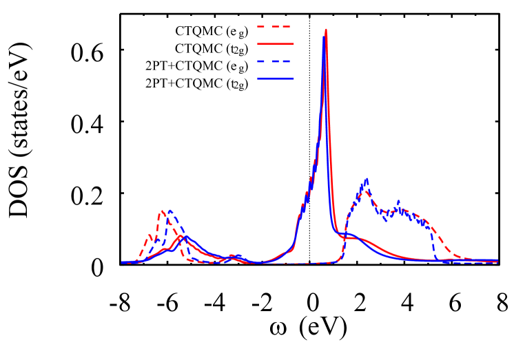
Figure 3: The calculated spectral function for SrVO₃ projected onto the V-$e_{\rm g}$ (dashed line) and $t_{\rm 2g}$ (solid line) orbitals. The result presented in red color is obtained with CTQMC solver for five V-$d$ orbitals. The blue colored lines present the result obtained by CTQMC solver for three V-$t_{\rm 2g}$ orbitals whose self-energy is then embedded into the second-order perturbation theory (2PT) solution.

One big advantage of using our NAO projector is to reliably separate the correlated subspace into two parts. It enables us to use an elaborate technique only for the one part of correlated orbitals while, for another part, a computationally cheaper approximation can be utilized. Or, high-level approximation can be adopted for both parts, which are then embedded by the self-energy obtained from the cheaper approximation as shown in recent model studies Kananenka et al. (2015); Nguyen Lan et al. (2016); Lan et al. (2017). In this scheme, natural orbitals were used as a basis set to represent the correlated subspace by taking only the orbitals whose occupations are close to 1.0.

We apply this type of capability to the first-principles DFT+DMFT framework. In order to see its effect, we extend the correlated subspace from three $t_{2g}$ orbitals to the $d$ complex (i.e., both $t_{2g}+e_{g}$). The former is certainly more relevant to the correlation effect and basically determines the most of electronic properties while the latter is less important. Therefore we adopted CTQMC solver for $t_{2g}$ orbitals and the second-order perturbation theory (2PT) for $e_{g}$, which significantly reduces the computation cost. For more details of our 2PT method, see Appendix A.

The calculation result of spectral function is presented as a blue line in Fig. 3. The red line in Fig. 3 represents the CTQMC-only result; namely, all of five V-$d$ orbitals are solved with CTQMC. In spite of much less computation cost (i.e., five- vs three-orbital impurity problem for CTQMC), the hybrid solver of 2PT+CTQMC gives a reasonable agreement with the CTQMC-only result especially for the near-$E_{F}$ region. For example, Hubbard bands and the $d$-$p$ hybridization part are well reproduced. Simultaneously, some deviations are also clearly noticed. For example, the intensity of the Hubbard bands are reduced in 2PT+CTQMC calculation. This reduced correlation in $t_{\rm 2g}$ manifolds is attributed to the inability of 2PT to accurately describe the screening effect Gukelberger et al. (2015); Honerkamp et al. (2018). As expected, the difference between the two computation results is more pronounced in high energy $e_{g}$ spectra.

III.3 NiO

As the second example, we chose a classical charge-transfer insulator NiO. Due to the sizable hybridization between Ni-$d$ and O-$p$, the electronic property depends on the choice of local correlated orbital projector. Note that the projector affects both Hubbard $U$ and charge-transfer energy $\Delta$ in this type of materials Zaanen et al. (1985); Wang et al. (2012); Dang et al. (2014). The inverse temperature of $\beta=10$ eV^-1 (corresponding to 1160.45 K higher than Neel temperature $T_{N}=525$ K Srinivasan and Seehra (1983); Roth (1958)) and the interaction parameters of $U=8$ eV and $J_{H}=1$ eV were used following the previous studies Karolak et al. (2010); Kuneš et al. (2007); Anisimov et al. (1991). Fig. 4 shows the electronic structures which were calculated by two different projectors; (a) PAO and (b) NAO. As expected, LDA ($U$=0; black solid line) gives the unphysical metallic solution while the experimental gap is $\sim$4.3 eV Hüfner et al. (1984).

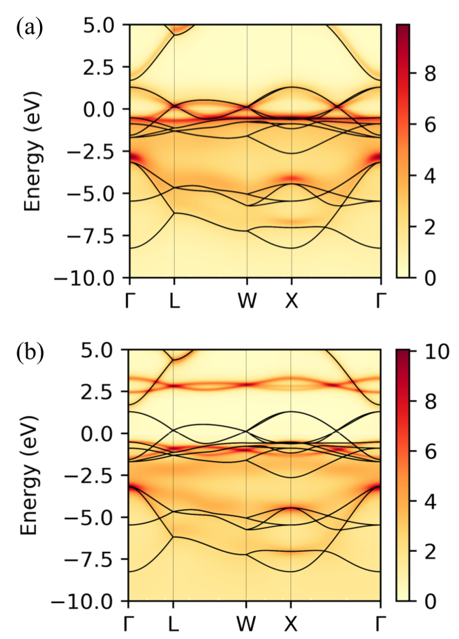
Figure 4: The calculated band dispersion of NiO. DFT+DMFT result (color map) is compared with that of LDA (black solid lines). Two different projection methods are adopted for DFT+DMFT calculation; (a) PAOs and (b) NAOs.

The DFT+DMFT spectral function $A({\bf k},\omega)$ calculated with PAO projector is presented as a false-color band in Fig. 4(a). Interestingly the system remains metallic in a sharp contrast to the previous calculations of DFT+$U$ Anisimov et al. (1991); Han et al. (2006) and DFT+DMFT Kuneš et al. (2007); Karolak et al. (2010). This result demonstrates the fact that the effect of correlations depend on the choice of local projector. Note that the Ni-${e_{g}}$ energy level $\epsilon^{e_{g}}=\braket{\hat{H}}_{\chi^{\rm PAOs}}=-7.58$ eV is significantly lower than that of NAO (see below) which results in the large number of Ni-$d$ electrons, $N_{d}=8.72$. In combination with the conventional FLL double counting, it leads to a significant change of chemical potential. This effect is clearly noticed, for example, in the bands at around $\pm\sim$2.5 eV being deviated from LDA bands.

The result of NAO projector is presented in Fig. 4(b) (false color plot) in comparison with LDA (black line). A well developed band gap is clearly identified. The on-site energy is significantly increased compared to PAO result, $\epsilon_{d}^{eg}=-7.21$ eV, and therefore the charge transfer energy is increased. The $d$ orbital occupancy is also reduced $N_{d}=8.21$. It is found that the electronic structure is overall quite consistent with previous theoretical studies Han et al. (2006); Karolak et al. (2010); Kuneš et al. (2007).

IV Summary

We introduce NAO as a local projector to define the correlated subspace in DFT+DMFT procedure. Our implementation is based on the systematic construction of projector from the original non-orthogonal PAO basis set. We apply this method to a correlated metal SrVO₃ and insulator NiO. From the comparison with other projector methods, we found that NAO not just serves as another possible choice, but it also has some advantage particularly in the charge counting. First, it provides a reliable electron number $N_{d}$ for the correlated orbitals and does not require any additional convergence or minimization procedure. No arbitrary numerical parameter needs to be introduced such as cut-off or muffin-tin radius, and the application to the entangled band structure is also straightforward. Finally, we emphasize that the use of NAO projector provides a viable way to separate correlated subspace into two parts; one for which the elaborate technique can be used for describing correlations, and for another part one can resort to a computationally cheaper approximation.

Appendix A Details of the second-order perturbation approach

Our DFT+DMFT iteration procedure with 2PT+CTQMC solver is summarized as follow.

(1) We start with the initial guess for self-energy $\Delta\Sigma(i\omega_{n})=\Sigma_{\text{weak}}+\Sigma_{\text{strong}}-\Sigma_{\text{DC}}^{\text{DFT}}=0$. The local Green’s function of a given material (or lattice problem) is

$$G_{\text{loc }}(i\omega_{n})=\frac{1}{N_{k}}\sum_{k}\left[i\omega_{n}-H_{k}+\mu-\Delta\Sigma(i\omega_{n})\right]^{-1}$$ (6)

where $H_{k}$ is the Kohn-Sham Hamiltonian and the chemical potential $\mu$ is adjusted to obtain the correct number of electrons.

(2) Calculate Weiss mean-field $\mathcal{G}^{-1}=G_{\text{loc}}^{-1}+\Sigma_{\text{imp}}$. Equivalently one can calculate the impurity energy level and the hybridization function from $H_{\text{imp}}=H_{\text{loc}}-\Sigma_{\text{DC}}^{\text{DFT}}$ and $\Delta=i\omega_{n}-H_{\text{loc}}+\mu-\Delta\Sigma-G_{\text{loc}}^{-1}$, respectively.

(3) Now we solve the impurity problem with an approximate way. Here we adopted the second-order perturbation theory:

$$\Sigma^{(2)}(i\omega_{n})=\Sigma^{\text{HF}}[G_{\text{loc}}]+\Sigma^{\prime(2)}[G_{\text{HF}}](i\omega_{n}),$$ (7)

where $\Sigma^{\text{HF}}$ is the Hartree-Fock contribution and

$$\Sigma_{ij}^{\prime(2)}[G](i\omega_{n})=(-G_{kl}(\tau)G_{mn}(\tau)G_{pq}(-\tau)+G_{kn}(\tau)G_{ml}(\tau)G_{pq}(-\tau))U_{iqmk}U_{lnpj}.$$ (8)

Here the summation over the repeated indices is assumed and $U_{ijkl}=\braket{ij}{U}{kl}$.

(4) Calculate the double counting term, $\Sigma_{\text{DC}}^{(2)}=\Sigma^{\text{HF}}[\hat{P}_{c}G_{\text{loc}}]+\Sigma^{\prime(2)}[\hat{P}_{c}G_{\text{HF}}](i\omega_{n}).$ Here $\hat{P}_{c}$ is the projector onto the strongly correlated orbitals, namely, $t_{\text{2g}}$ orbitals for SVO₃. Then we have $\Sigma_{\text{weak}}(i\omega_{n})=\Sigma^{(2)}(i\omega_{n})-\Sigma_{\text{DC}}^{(2)}(i\omega_{n})$.

(5) CTQMC impurity solver is adopted to obtain the impurity self-energy $\Sigma_{\text{strong}}$ describing the correlated subspace $c$. Again, we construct the impurity problem from the Weiss field $\mathcal{G_{\text{strong}}}^{-1}=(P_{c}G_{\text{loc}})^{-1}+\Sigma_{\text{strong}}$. Alternatively, we can define the impurity site energy $H_{\text{imp}}^{\text{strong}}=H_{\text{loc}}+\Sigma_{\text{weak}}(\infty)-\Sigma_{\text{DC}}^{\text{DFT}}$ and the hybridization $\Delta_{\text{strong}}=i\omega_{n}-H_{\text{imp}}^{\text{strong}}+\mu-\Sigma_{\text{strong}}-(P_{c}G_{\text{loc}})^{-1}\approx i\omega_{n}-H_{\text{loc}}+\mu-P_{c}(\Delta\Sigma)+\Sigma_{\text{weak}}^{\prime}-(P_{c}G_{\text{loc}})^{-1}.$

(6) Update $\Delta\Sigma(i\omega_{n})=\Sigma_{\text{weak}}+\Sigma_{\text{strong}}-\Sigma_{\text{DC}}^{\text{DFT}}$ and go back to step 2.

References

- Anisimov et al. (1991) Vladimir I. Anisimov, Jan Zaanen, and Ole K. Andersen, “Band theory and Mott insulators: Hubbard instead of Stoner ,” Phys. Rev. B 44, 943 (1991).
- Anisimov et al. (1993) V. I. Anisimov, I. V. Solovyev, M. A. Korotin, M. T. Czyżyk, and G. A. Sawatzky, “Density-functional theory and NiO photoemission spectra,” Phys. Rev. B 48, 16929 (1993).
- Ho et al. (2008) K. M. Ho, J. Schmalian, and C. Z. Wang, “Gutzwiller density functional theory for correlated electron systems,” Phys. Rev. B 77, 073101 (2008).
- Gutzwiller (1965) Martin C. Gutzwiller, “Correlation of Electrons in a Narrow Band,” Phys. Rev. 137, A1726 (1965).
- Deng et al. (2009) XiaoYu Deng, Lei Wang, Xi Dai, and Zhong Fang, “Local density approximation combined with Gutzwiller method for correlated electron systems: Formalism and applications,” Phys. Rev. B 79, 075114 (2009).
- Lanatà et al. (2015) Nicola Lanatà, Yongxin Yao, Cai-Zhuang Wang, Kai-Ming Ho, and Gabriel Kotliar, “Phase Diagram and Electronic Structure of Praseodymium and Plutonium,” Phys. Rev. X 5, 011008 (2015).
- van Schilfgaarde et al. (2006) M. van Schilfgaarde, Takao Kotani, and S. Faleev, “Quasiparticle Self-Consistent Theory,” Phys. Rev. Lett. 96, 226402 (2006).
- Kotani et al. (2007) Takao Kotani, Mark van Schilfgaarde, and Sergey V. Faleev, “Quasiparticle self-consistent method: A basis for the independent-particle approximation,” Phys. Rev. B 76, 165106 (2007).
- Faleev et al. (2004) Sergey V. Faleev, Mark van Schilfgaarde, and Takao Kotani, “All-Electron Self-Consistent Approximation: Application to Si, MnO, and NiO,” Phys. Rev. Lett. 93, 126406 (2004).
- Jang et al. (2015) Seung Woo Jang, Takao Kotani, Hiori Kino, Kazuhiko Kuroki, and Myung Joon Han, “Quasiparticle self-consistent GW study of cuprates: Electronic structure, model parameters, and the two-band theory for Tc,” Sci. Rep. 5, 12050 (2015).
- Ryee et al. (2016) Siheon Ryee, Seung Woo Jang, Hiori Kino, Takao Kotani, and Myung Joon Han, “Quasiparticle self-consistent GW calculation of Sr2RuO4 and SrRuO3,” Phys. Rev. B 93, 075125 (2016).
- Georges and Kotliar (1992) Antoine Georges and Gabriel Kotliar, “Hubbard model in infinite dimensions,” Phys. Rev. B 45, 6479 (1992).
- Metzner and Vollhardt (1989) Walter Metzner and Dieter Vollhardt, “Correlated Lattice Fermions in Dimensions,” Phys. Rev. Lett. 62, 324 (1989).
- Zhang et al. (1993) X. Y. Zhang, M. J. Rozenberg, and G. Kotliar, “Mott transition in the Hubbard model at zero temperature,” Phys. Rev. Lett. 70, 1666 (1993).
- Anisimov et al. (1997) V. I. Anisimov, A. I. Poteryaev, M. A. Korotin, A. O. Anokhin, and G. Kotliar, “First-principles Calculations of the Electronic Structure and Spectra of Strongly Correlated Systems: Dynamical Mean-field Theory,” J Phys Condens Matter 9, 7359 (1997).
- Lichtenstein and Katsnelson (1998) A. I. Lichtenstein and M. I. Katsnelson, “Ab initio calculations of quasiparticle band structure in correlated systems: LDA++ approach,” Phys. Rev. B 57, 6884 (1998).
- Kotliar et al. (2006) G. Kotliar, S. Y. Savrasov, K. Haule, V. S. Oudovenko, O. Parcollet, and C. A. Marianetti, “Electronic structure calculations with dynamical mean-field theory,” Rev. Mod. Phys. 78, 865 (2006).
- Georges et al. (1996) Antoine Georges, Gabriel Kotliar, Werner Krauth, and Marcelo J. Rozenberg, “Dynamical mean-field theory of strongly correlated fermion systems and the limit of infinite dimensions,” Rev. Mod. Phys. 68, 13 (1996).
- Amadon et al. (2008) B. Amadon, F. Lechermann, A. Georges, F. Jollet, T. O. Wehling, and A. I. Lichtenstein, “Plane-wave based electronic structure calculations for correlated materials using dynamical mean-field theory and projected local orbitals,” Phys. Rev. B 77, 205112 (2008).
- Anisimov et al. (2005) V. I. Anisimov, D. E. Kondakov, A. V. Kozhevnikov, I. A. Nekrasov, Z. V. Pchelkina, J. W. Allen, S. K. Mo, H. D. Kim, P. Metcalf, S. Suga, A. Sekiyama, G. Keller, I. Leonov, X. Ren, and D. Vollhardt, “Full orbital calculation scheme for materials with strongly correlated electrons,” Phys. Rev. B 71, 125119 (2005).
- Savrasov et al. (2001) S. Y. Savrasov, G. Kotliar, and E. Abrahams, “Correlated electrons in -plutonium within a dynamical mean-field picture,” Nature 410, 793 (2001).
- Held et al. (2001a) K. Held, A. K. McMahan, and R. T. Scalettar, “Cerium Volume Collapse: Results from the Merger of Dynamical Mean-Field Theory and Local Density Approximation,” Phys. Rev. Lett. 87, 276404 (2001a).
- Held et al. (2001b) K. Held, G. Keller, V. Eyert, D. Vollhardt, and V. I. Anisimov, “Mott-Hubbard Metal-Insulator Transition in Paramagnetic V2O3: An Study,” Phys. Rev. Lett. 86, 5345 (2001b).
- Park et al. (2008) H. Park, K. Haule, and G. Kotliar, “Cluster Dynamical Mean Field Theory of the Mott Transition,” Phys. Rev. Lett. 101, 186403 (2008).
- de’ Medici et al. (2011) Luca de’ Medici, Jernej Mravlje, and Antoine Georges, “Janus-Faced Influence of Hund’s Rule Coupling in Strongly Correlated Materials,” Phys. Rev. Lett. 107, 256401 (2011).
- Kent and Kotliar (2018) Paul R. C. Kent and Gabriel Kotliar, “Toward a predictive theory of correlated materials,” Science 361, 348–354 (2018).
- Choi et al. (2019) Sangkook Choi, Patrick Semon, Byungkyun Kang, Andrey Kutepov, and Gabriel Kotliar, “ComDMFT: A massively parallel computer package for the electronic structure of correlated-electron systems,” Comput. Phys. Commun. 244, 277 (2019).
- (28) “DMFTpack,” https://kaist-elst.github.io/DMFTpack/.
- Alet et al. (2005) F. Alet, P. Dayal, A. Grzesik, A. Honecker, M. K orner, A. L auchli, S. R. Manmana, I. P. McCulloch, F. Michel, R. M. Noack, G. Schmid, U. Schollwöck, F. Stöckli, S. Todo, S. Trebst, M. Troyer, P. Werner, and S. Wessel, “The ALPS project release 2.0: Open source software for strongly correlated systems,” J Phys Soc Jpn 74, 30 (2005).
- Parcollet et al. (2015) Olivier Parcollet, Michel Ferrero, Thomas Ayral, Hartmut Hafermann, Igor Krivenko, Laura Messio, and Priyanka Seth, “TRIQS: A toolbox for research on interacting quantum systems,” Computer Physics Communications 196, 398 (2015).
- Haule et al. (2010) Kristjan Haule, Chuck-Hou Yee, and Kyoo Kim, “Dynamical mean-field theory within the full-potential methods: Electronic structure of CeIrIn5, CeCoIn5, and CeRhIn5,” Phys. Rev. B 81, 195107 (2010).
- Souza et al. (2001) Ivo Souza, Nicola Marzari, and David Vanderbilt, “Maximally-localized Wannier functions for entangled energy bands,” Phys. Rev. B 65, 035109 (2001).
- Marzari and Vanderbilt (1997) Nicola Marzari and David Vanderbilt, “Maximally localized generalized Wannier functions for composite energy bands,” Phys. Rev. B 56, 12847 (1997).
- Andersen and Saha-Dasgupta (2000) O. K. Andersen and T. Saha-Dasgupta, “Muffin-tin orbitals of arbitrary order,” Phys. Rev. B 62, R16219 (2000).
- Pavarini et al. (2004) E. Pavarini, S. Biermann, A. Poteryaev, A. I. Lichtenstein, A. Georges, and O. K. Andersen, “Mott Transition and Suppression of Orbital Fluctuations in Orthorhombic Perovskites,” Phys. Rev. Lett. 92, 176403 (2004).
- Haule et al. (2014) Kristjan Haule, Turan Birol, and Gabriel Kotliar, “Covalency in transition-metal oxides within all-electron dynamical mean-field theory,” Phys. Rev. B 90, 075136 (2014).
- Wang et al. (2012) Xin Wang, M. J. Han, Luca De’Medici, Hyowon Park, C. A. Marianetti, and Andrew J. Millis, “Covalency, double-counting, and the metal-insulator phase diagram in transition metal oxides,” Phys. Rev. B 86, 195136 (2012).
- Dang et al. (2014) Hung T. Dang, Andrew J. Millis, and Chris A. Marianetti, “Covalency and the metal-insulator transition in titanate and vanadate perovskites,” Phys. Rev. B 89, 161113(R) (2014).
- Mulliken (1955a) R. S. Mulliken, “Electronic Population Analysis on LCAO–MO Molecular Wave Functions. I,” J. Chem. Phys. 23, 1833 (1955a).
- Mulliken (1955b) R. S. Mulliken, “Electronic Population Analysis on LCAO–MO Molecular Wave Functions. II. Overlap Populations, Bond Orders, and Covalent Bond Energies,” J. Chem. Phys. 23, 1841 (1955b).
- Löwdin (1950) Per Olov Löwdin, “On the non-orthogonality problem connected with the use of atomic wave functions in the theory of molecules and crystals,” J Chem Phys 18, 365 (1950).
- Reed et al. (1985) Alan E. Reed, Robert B. Weinstock, and Frank Weinhold, “Natural population analysis,” J. Chem. Phys. 83, 735 (1985).
- (43) “OpenMX,” http://www.openmx-square.org.
- Werner et al. (2006) Philipp Werner, Armin Comanac, Luca de’ Medici, Matthias Troyer, and Andrew J. Millis, “Continuous-Time Solver for Quantum Impurity Models,” Phys. Rev. Lett. 97, 076405 (2006).
- Werner and Millis (2006) Philipp Werner and Andrew J. Millis, “Hybridization expansion impurity solver: General formulation and application to Kondo lattice and two-orbital models,” Phys. Rev. B 74, 155107 (2006).
- Koch et al. (2008) Erik Koch, Giorgio Sangiovanni, and Olle Gunnarsson, “Sum rules and bath parametrization for quantum cluster theories,” Phys. Rev. B 78, 115102 (2008).
- Caffarel and Krauth (1994) Michel Caffarel and Werner Krauth, “Exact diagonalization approach to correlated fermions in infinite dimensions: Mott transition and superconductivity,” Phys. Rev. Lett. 72, 1545 (1994).
- Wilson (1975) Kenneth G. Wilson, “The renormalization group: Critical phenomena and the Kondo problem,” Rev. Mod. Phys. 47, 773–840 (1975).
- Bulla et al. (2008) Ralf Bulla, Theo A. Costi, and Thomas Pruschke, “Numerical renormalization group method for quantum impurity systems,” Rev. Mod. Phys. 80, 395 (2008).
- Bauernfeind et al. (2017) Daniel Bauernfeind, Manuel Zingl, Robert Triebl, Markus Aichhorn, and Hans Gerd Evertz, “Fork tensor-product states: Efficient multiorbital real-time DMFT solver,” Phys Rev X 7, 031013 (2017).
- Karolak et al. (2010) M. Karolak, G. Ulm, T. Wehling, V. Mazurenko, A. Poteryaev, and A. Lichtenstein, “Double counting in LDA+DMFT—The example of NiO,” J. Electron Spectrosc. Relat. Phenom. 181, 11 (2010).
- Haule (2015) Kristjan Haule, “Exact Double Counting in Combining the Dynamical Mean Field Theory and the Density Functional Theory,” Phys. Rev. Lett. 115, 196403 (2015).
- Lechermann et al. (2006) F. Lechermann, A. Georges, A. Poteryaev, S. Biermann, M. Posternak, A. Yamasaki, and O. K. Andersen, “Dynamical mean-field theory using Wannier functions: A flexible route to electronic structure calculations of strongly correlated materials,” Phys. Rev. B 74, 125120 (2006).
- Bhandary et al. (2016) Sumanta Bhandary, Elias Assmann, Markus Aichhorn, and Karsten Held, “Charge self-consistency in density functional theory combined with dynamical mean field theory: -space reoccupation and orbital order,” Phys. Rev. B 94, 155131 (2016).
- (55) “DCore,” https://issp-center-dev.github.io/DCore/.
- L. V. Pourovskii et al. (2007) L. V. Pourovskii, B. Amadon, S. Biermann, and A. Georges, “Self-consistency over the charge density in dynamical mean-field theory: A linear muffin-tin implementation and some physical implications,” Phys. Rev. B 76, 235101 (2007).
- Amadon (2012) B. A. Amadon, “A self-consistent DFT+DMFT scheme in the projector augmented wave method: Applications to cerium, Ce2O3 and Pu2O3 with the Hubbard I solver and comparison to DFT,” J Phys Condens Matter 24, 075604 (2012).
- Aichhorn et al. (2009) Markus Aichhorn, Leonid Pourovskii, Veronica Vildosola, Michel Ferrero, Olivier Parcollet, Takashi Miyake, Antoine Georges, and Silke Biermann, “Dynamical mean-field theory within an augmented plane-wave framework: Assessing electronic correlations in the iron pnictide LaFeAsO,” Phys. Rev. B 80, 085101 (2009).
- Karolak et al. (2011) M Karolak, T O Wehling, F Lechermann, and A I Lichtenstein, “General DFT++ method implemented with projector augmented waves: Electronic structure of SrVO3 and the Mott transition in Ca2-SrRuO4,” J. Phys. Condens. Matter 23, 085601 (2011).
- Schüler et al. (2018) M Schüler, O E Peil, G J Kraberger, R Pordzik, M Marsman, G Kresse, T O Wehling, and M Aichhorn, “Charge self-consistent many-body corrections using optimized projected localized orbitals,” J. Phys.: Condens. Matter 30, 475901 (2018).
- Kananenka et al. (2015) Alexei A. Kananenka, Emanuel Gull, and Dominika Zgid, “Systematically improvable multiscale solver for correlated electron systems,” Phys. Rev. B 91, 121111(R) (2015).
- Ozaki and Kino (2004) T. Ozaki and H. Kino, “Numerical atomic basis orbitals from H to Kr,” Phys. Rev. B 69, 195113 (2004).
- Ozaki (2003) T. Ozaki, “Variationally optimized atomic orbitals for large-scale electronic structures,” Phys. Rev. B 67, 155108 (2003).
- Han et al. (2006) Myung Joon Han, Taisuke Ozaki, and Jaejun Yu, “O() LDA+ electronic structure calculation method based on the nonorthogonal pseudoatomic orbital basis,” Phys. Rev. B 73, 045110 (2006).
- Löwdin (1955) Per-Olov Löwdin, “Quantum Theory of Many-Particle Systems. I. Physical Interpretations by Means of Density Matrices, Natural Spin-Orbitals, and Convergence Problems in the Method of Configurational Interaction,” Phys. Rev. 97, 1474 (1955).
- Reed et al. (1988) Alan E. Reed, Larry A. Curtiss, and Frank Weinhold, “Intermolecular interactions from a natural bond orbital, donor-acceptor viewpoint,” Chem. Rev. 88, 899 (1988).
- Go and Millis (2017) Ara Go and Andrew J. Millis, “Adaptively truncated Hilbert space based impurity solver for dynamical mean-field theory,” Phys. Rev. B 96, 085139 (2017).
- Mayda et al. (2017) Selma Mayda, Zafer Kandemir, and Nejat Bulut, “Electronic Structure of Cyanocobalamin: DFT+QMC Study,” J Supercond Nov Magn 30, 3301 (2017).
- Perdew and Zunger (1981) J. P. Perdew and Alex Zunger, “Self-interaction correction to density-functional approximations for many-electron systems,” Phys. Rev. B 23, 5048–5079 (1981).
- Ceperley and Alder (1980) D. M. Ceperley and B. J. Alder, “Ground State of the Electron Gas by a Stochastic Method,” Phys. Rev. Lett. 45, 566 (1980).
- Rey et al. (1990) M. J. Rey, Ph Dehaudt, J. C. Joubert, B. Lambert-Andron, M. Cyrot, and F. Cyrot-Lackmann, “Preparation and structure of the compounds SrVO3 and Sr2VO4,” J Solid State Chem 86, 101 (1990).
- Furstenau et al. (1985) R.P. Furstenau, G. McDougall, and M.A. Langell, “Initial stages of hydrogen reduction of NiO(100),” Surface Science 150, 55 (1985).
- Gull et al. (2001) E. Gull, A. J. Millis, A. I. Lichtenstein, A. N. Rubtsov, M. Troyer, and P. Werner, “Continuous-time Monte Carlo methods for quantum impurity models,” Rev. Mod. Phys. 83, 349 (2001).
- Gull et al. (2011) Emanuel Gull, Philipp Werner, Sebastian Fuchs, Brigitte Surer, Thomas Pruschke, and Matthias Troyer, “Continuous-time quantum Monte Carlo impurity solvers,” Comput. Phys. Commun. 182, 1078 (2011).
- Haule (2007) Kristjan Haule, “Quantum Monte Carlo impurity solver for cluster dynamical mean-field theory and electronic structure calculations with adjustable cluster base,” Phys. Rev. B 75, 155113 (2007).
- (76) http://hauleweb.rutgers.edu/tutorials/Tutorial0.html.
- Jarrell and Gubernatis (1996) M. Jarrell and J. E. Gubernatis, “Bayesian inference and the analytic continuation of imaginary-time quantum Monte Carlo data,” Phys. Rep. 269, 133 (1996).
- Gunnarsson et al. (2010) O. Gunnarsson, M. W. Haverkort, and G. Sangiovanni, “Analytical continuation of imaginary axis data using maximum entropy,” Phys. Rev. B 81, 155107 (2010).
- Sim and Han (2018) Jae-Hoon Sim and Myung Joon Han, “Maximum quantum entropy method,” Phys. Rev. B 98, 205102 (2018).
- Nekrasov et al. (2005) I. A. Nekrasov, G. Keller, D. E. Kondakov, A. V. Kozhevnikov, Th. Pruschke, K. Held, D. Vollhardt, and V. I. Anisimov, “Comparative study of correlation effects in CaVO3 and SrVO3,” Phys. Rev. B 72, 155106 (2005).
- Nekrasov et al. (2006) I. A. Nekrasov, K. Held, G. Keller, D. E. Kondakov, Th. Pruschke, M. Kollar, O. K. Andersen, V. I. Anisimov, and D. Vollhardt, “Momentum-resolved spectral functions of SrVO3 calculated by LDA+DMFT,” Phys. Rev. B 73, 155112 (2006).
- Sekiyama et al. (2004) A. Sekiyama, H. Fujiwara, S. Imada, S. Suga, H. Eisaki, S. I. Uchida, K. Takegahara, H. Harima, Y. Saitoh, I. A. Nekrasov, G. Keller, D. E. Kondakov, A. V. Kozhevnikov, Th. Pruschke, K. Held, D. Vollhardt, and V. I. Anisimov, “Mutual Experimental and Theoretical Validation of Bulk Photoemission Spectra of Sr1-xCaxVO3,” Phys. Rev. Lett. 93, 156402 (2004).
- Nomura et al. (2012) Yusuke Nomura, Merzuk Kaltak, Kazuma Nakamura, Ciro Taranto, Shiro Sakai, Alessandro Toschi, Ryotaro Arita, Karsten Held, Georg Kresse, and Masatoshi Imada, “Effective on-site interaction for dynamical mean-field theory,” Phys. Rev. B 86, 085117 (2012).
- Lee et al. (2012) Hunpyo Lee, Kateryna Foyevtsova, Johannes Ferber, Markus Aichhorn, Harald O. Jeschke, and Roser Valentí, “Dynamical cluster approximation within an augmented plane wave framework: Spectral properties of SrVO3,” Phys. Rev. B 85, 165103 (2012).
- Taranto et al. (2013) C. Taranto, M. Kaltak, N. Parragh, G. Sangiovanni, G. Kresse, A. Toschi, and K. Held, “Comparing quasiparticle GW+DMFT and LDA+DMFT for the test bed material SrVO3,” Phys. Rev. B 88, 165119 (2013).
- Casula et al. (2012) Michele Casula, Alexey Rubtsov, and Silke Biermann, “Dynamical screening effects in correlated materials: Plasmon satellites and spectral weight transfers from a Green’s function ansatz to extended dynamical mean field theory,” Phys. Rev. B 85, 035115 (2012).
- Tomczak et al. (2014) Jan M. Tomczak, M. Casula, T. Miyake, and S. Biermann, “Asymmetry in band widening and quasiparticle lifetimes in SrVO3 : Competition between screened exchange and local correlations from combined and dynamical mean-field theory +DMFT,” Phys. Rev. B 90, 165138 (2014).
- Tomczak et al. (2012) Jan M. Tomczak, Michele Casula, Takashi Miyake, Ferdi Aryasetiawan, and Silke Biermann, “Combined GW and dynamical mean-field theory: Dynamical screening effects in transition metal oxides,” EPL Europhys. Lett. 100, 67001 (2012).
- Choi et al. (2016) Sangkook Choi, Andrey Kutepov, Kristjan Haule, Mark van Schilfgaarde, and Gabriel Kotliar, “First-principles treatment of Mott insulators: Linearized QSGW+DMFT approach,” Npj Quantum Materials 1, 16001 (2016).
- Yoshida et al. (2005) T. Yoshida, K. Tanaka, H. Yagi, A. Ino, H. Eisaki, A. Fujimori, and Z.-X. Shen, “Direct Observation of the Mass Renormalization in SrVO3 by Angle Resolved Photoemission Spectroscopy,” Phys. Rev. Lett. 95, 146404 (2005).
- Nguyen Lan et al. (2016) Tran Nguyen Lan, Alexei A. Kananenka, and Dominika Zgid, “Rigorous Ab Initio Quantum Embedding for Quantum Chemistry Using Green’s Function Theory: Screened Interaction, Nonlocal Self-Energy Relaxation, Orbital Basis, and Chemical Accuracy,” J Chem Theory Comput 12, 4856 (2016).
- Lan et al. (2017) Tran Nguyen Lan, Avijit Shee, Jia Li, Emanuel Gull, and Dominika Zgid, “Testing self-energy embedding theory in combination with GW,” Phys. Rev. B 96, 155106 (2017).
- Gukelberger et al. (2015) Jan Gukelberger, Li Huang, and Philipp Werner, “On the dangers of partial diagrammatic summations: Benchmarks for the two-dimensional Hubbard model in the weak-coupling regime,” Phys. Rev. B 91, 235114 (2015).
- Honerkamp et al. (2018) Carsten Honerkamp, Hiroshi Shinaoka, Fakher F. Assaad, and Philipp Werner, “Limitations of constrained random phase approximation downfolding,” Phys. Rev. B 98, 235151 (2018).
- Zaanen et al. (1985) J. Zaanen, G. A. Sawatzky, and J. W. Allen, “Band gaps and electronic structure of transition-metal compounds,” Phys. Rev. Lett. 55, 418 (1985).
- Srinivasan and Seehra (1983) G. Srinivasan and Mohindar S. Seehra, “Nature of magnetic transitions in MnO, FezO, CoO, and NiO,” Phys. Rev. B 28, 6542 (1983).
- Roth (1958) W. L. Roth, “Multispin Axis Structures for Antiferromagnets,” Phys. Rev. 111, 772 (1958).
- Kuneš et al. (2007) J. Kuneš, V. I. Anisimov, A. V. Lukoyanov, and D. Vollhardt, “Local correlations and hole doping in NiO: A dynamical mean-field study,” Phys. Rev. B 75, 165115 (2007).
- Hüfner et al. (1984) S. Hüfner, J. Osterwalder, T. Riesterer, and F. Hulliger, “Photoemission and inverse photoemission spectroscopy of NiO,” Solid State Commun. 52, 793 (1984).