Short-Term Load Forecasting Using AMI Data

Abstract

Accurate short-term load forecasting is essential for the efficient operation of the power sector. Forecasting load at a fine granularity such as hourly loads of individual households is challenging due to higher volatility and inherent stochasticity. At the aggregate levels, such as monthly load at a grid, the uncertainties and fluctuations are averaged out; hence predicting load is more straightforward. This paper proposes a method called Forecasting using Matrix Factorization (fmf) for short-term load forecasting (stlf). fmf only utilizes historical data from consumers’ smart meters to forecast future loads (does not use any non-calendar attributes, consumers’ demographics or activity patterns information, etc.) and can be applied to any locality. A prominent feature of fmf is that it works at any level of user-specified granularity, both in the temporal (from a single hour to days) and spatial dimensions (a single household to groups of consumers). We empirically evaluate fmf on three benchmark datasets and demonstrate that it significantly outperforms the state-of-the-art methods in terms of load forecasting. The computational complexity of fmf is also substantially less than known methods for stlf such as long short-term memory neural networks, random forest, support vector machines, and regression trees.

I Introduction

Smart grid is a communication and control network on top of the electric grid to collect and analyze data from iot devices at various grid elements. A fundamental task in power systems management is to accurately predict consumers’ electricity demands based on past loads collected from smart meters. Inaccuracy in the demand estimate and the subsequent operational decisions may result in grid instability and sub-optimal resource utilization entailing high economic costs. Long-Term Load Forecasting (a few months to a year) is needed for power infrastructure planning [1]. However, operational decisions for smart grids have to be made within a short time and require Short-Term Load Forecasting (stlf) (a few hours to days) [2]. Renewable energy resources are inherently intermittent in nature [3, 4], with their increasing integration in the energy mix, accurate stlf becomes even more crucial [5].

Load forecasting can be categorized based on the spatial granularity of forecast, ranging from large scale (e.g., feeders or grids level) to fine-scale (e.g., individual consumer or household level). Forecasting at a smaller scale is more challenging due to the interplay of many factors [6, 5, 7, 8]. Most of these factors are unknown or hard to measure, such as demographics, number, and daily schedules of residents in a household. It is well known that with increasing spatial aggregation, the forecasting error decreases [9, 7]. This behavior is because many fluctuations tend to average out at larger scales.

A wide variety of methods have been proposed for stlf at large scales. These methods apply statistical and machine learning techniques to historical load data to predict the (total) load of all consumers [1, 10, 11, 12]. However, efficient and accurate load forecasting for short-term and at a fine scale is pivotal for demand response programs [1, 9, 2], peak shaving [10, 13], dynamic pricing [14] and soft load-shedding schemes [15, 16].

In the Advanced Metering Infrastructure (ami), consumers are increasingly connected to the grid through smart meters, a typical example of iot. Over 100 million smart meters have been installed in the USA [17]. ami makes available short duration load data for individual consumers. There is an increasing research interest in utilizing this data for stlf to optimize power system management [13, 8].

Most recent works on stlf group consumers into clusters based on their load profiles (hourly ami readings) and sociological data (obtained from surveys). Then the load of each cluster is predicted using machine learning methods [18, 19, 20, 21]. The survey data is not necessarily reliable when available and limits the applicability of the methods to a specific locality. Moreover, the total load of a cluster is smoother and less volatile (Figure 1), hence relatively easier to forecast.

Figure 1: (a) Hourly load of a randomly selected household in Sweden dataset for a single day (Fri, $5$ Jan, $2004$). (b) Total hourly load of all households for the same day.

In this paper, we propose an algorithm called Forecasting using Matrix Factorization (fmf) for short-term load forecasting at any user-specified level of spatial and temporal granularity. We perform a comprehensive exploratory analysis of three benchmark datasets from three countries to visually observe patterns in the data. fmf first applies data transformation on the past load values to reduce skewness in the data. Since the dimensionality of data is high, to avoid the ”curse of dimensionality”, we factorize the load matrix using Singular Value Decomposition (svd) to get a low-dimensional representation both for time-stamps (hour) and consumers. The new feature vectors for time-stamps are based on all consumers’ overall behavior in that hour. Similarly, the feature vectors of consumers are determined by their consumption patterns for the total period of the training data. (Note that we use the word consumer and household interchangeably throughout the paper). We empirically demonstrate that this representation improves the forecasting performance of our model. In this feature space, we aggregate hours into demonstrably more meaningful clusters. Finally, to predict the load of a consumer in a query hour (in the test set), we find clusters of hours in the training data that are ‘most similar’ to the query hour and report an ‘average’ of the consumer’s loads in those clusters.

We perform an extensive empirical evaluation of fmf to showcase its efficacy as a general-purpose forecasting method that works for a wide range of user-specified spatial and temporal granularity. We compare fmf with baseline and state-of-the-art (sota) methods using their respective experimental setup and evaluation metric. We show that fmf significantly outperforms known methods on stlf at the individual consumer level. We test fmf on forecasting loads for longer durations (up to a day), for groups (clusters) of consumers, and both combined. Results reveal that the performance of fmf surpasses the computationally expensive specialized methods for these tasks.

Key features of fmf are the following:

• fmf only utilizes the readily available hourly electricity consumption ami data and does not require any consumers specific information. Hence fmf is more generally applicable.

• fmf works at any level of user-specified granularity, both in the temporal and spatial dimensions.

• fmf does not require any complex training of the model, unlike Long Short Term Memory (lstm), Random Forest (rf), Support Vector Machine (svm), and Regression Tree (rt). Thus fmf is more suitable for stlf, where timely decisions need to be made.

• fmf achieves up to $26.5\%$ and $24.4\%$ improvement in Root Mean Square Error (rmse) over svr and rt, respectively and up to $73.8\%$ and $38\%$ improvement in Mean Absolute Percentage Error (mape) over rf and lstm, respectively.

• The representations learned for consumers and time-steps in our model preserves the overall structure of data, reduce the computational complexity of the model, and make the model scalable to big data.

The rest of the paper is organized as follows. We provide a brief review of existing methods for stlf in Section II. In Section III we describe the fmf scheme. Section IV contains datasets description and experimental setup. Results of empirical evaluation and comparisons of fmf are reported in Section V. Finally, we conclude the paper in Section VI.

II Related Work

The existing work on stlf can be divided into three categories, namely (i) stlf at system or subsystem level in which aggregated the load of all consumers at a locality is forecasted, (ii) Clusters level stlf, where consumers are intelligently grouped into clusters and loads for those clusters are forecasted, and (iii) stlf for individual consumers in which load is forecasted separately for each customer.

II-A stlf at System or Subsystem Level

Short-term load forecasting at a system/subsystem level is well explored in the literature. A neural network based method for stlf is proposed in [22] in which households are grouped based on location, nature, and size of loads. In [23] $k$-nearest neighbors based algorithm is used to forecast day-ahead loads of groups of consumers. A framework using wavelet transform and Bayesian neural network for stlf at the system level is proposed in [24]. A time-series method using intra-day and intra-week seasonal cycles is proposed in [25] for forecasting country loads a few minutes ahead. In [26], stochastic properties of electricity in France are utilized to predict short-term aggregated load. A kernel-based support vector regression model for the stlf at system level is proposed in [27]. A hybrid machine learning model is proposed in [28], which uses the combination of arima, logistic regression, and artificial neural networks to forecast day-ahead peak electric load at the system level. Several authors proposed hybrid methods involving data preprocessing with classification, regression, and other machine learning based methods for stlf at system/subsystem level [29, 5].

There are several problems with directly using machine learning models for stlf, such as difficulties in parameter selection and non-obvious selection of input variables [30]. Therefore, these models have to be combined with statistical models and different data preprocessing techniques to reduce the computational overhead. Authors in [30] use a combination of neural network and statistical models for stlf at microgrid level. An unsupervised machine learning model is proposed in [31], which combines Auto Correlation Function and Least Squares Support Vector Machines model to forecast short term load at the system level. The actual deployability of the forecasting algorithms at the country level is studied in [32]. The authors focus on prediction power, the robustness of model, the dependence of model on the dataset, and storage size. Multiple wavelet convolution neural networks are proposed, which balance these measures. Since the impact of variables on the demand changes over time, an online continuous learning approach is proposed and tested by [33]. The author used correlation analysis to figure out the effect of variables and then used a neural network for prediction in an online setting.

II-B stlf for Clusters of Consumers

A wide variety of methods utilize the increasingly available ami data to intelligently group the households into clusters (based on their consumption patterns) and forecast the load of these clusters. For cluster loads prediction, machine learning models such as random forest, neural networks, and deep learning are commonly used. Clustering is accomplished based on similarities in load profiles (consumers’ ami readings) [21] and consumers demographic information [20]. Practice theory of human behavior is incorporated for improved clustering [34], resulting in an accuracy boost for day-ahead system-level load forecast. A deep neural network-based model for stlf at an individual and subsystem level is proposed in [35], which learns complex relations between weather, calendar, and previous consumption for individual households. A hybrid approach consisting of a convolutional neural network and $k$-means clustering algorithm is proposed in [36] to forecast the hourly load of clusters of households. In [37] the authors propose a multi-resolution clustering method to forecast half hourly load for households. The relationship between cluster size and forecast accuracy is studied in [38] using two forecasting methods, namely Holt-Winters and Seasonal Naive.

II-C stlf for Individual Consumers

stlf at individual consumers’ level is significantly more challenging due to high volatility and variability in load profiles [39]. The classical methods treat each consumers’ data as a stationary time series for prediction. Time series methods for stlf use Kalman filter [40], advanced statistical techniques [41], and the standard Auto Regressive Integrated Moving Average (arima) forecasting models [10]. These time series approaches, however, do not capture the complex nonlinear relationship between electricity consumption and periodic routines of household residents [19]. It has been shown in [42] that time series based methods hardly beat persistent forecast (using previous hour load value as the forecast for the next hour). Authors in [43] propose a regression based method to forecast the monthly aggregated load of individual households. However, they do not take into account the temporal order of the historical loads in which the load values were observed. This limitation restricts the application of the method in any realistic scenario. A Pooling based deep recurrent neural network method is proposed in [10] to predict individual households loads and improve upon the accuracy of arima, and other machine learning models. Similarly, [9] uses lstm network along with density based clustering for household load forecasting. Authors in [44] used a factored conditional restricted Boltzmann machine for load forecasting of buildings and showed improvement over the support vector machine and neural network. A stlf model for individual household level is proposed in [39], which uses standard machine learning models such as neural networks and svm for load forecasting. [45] proposes a model for stlf, which uses historical loads and weather information along with the information contained in typical daily consumption profiles (loads in mornings, evenings, and nights, etc.) for load forecasting. A predicted model (sparse high-dimensional partially linear additive models) for stlf at individual households level is used in [7], which forecasts half-hourly electricity load for one day ahead. In [46], the authors propose a clustering based method, which uses historical load to forecast day ahead loads of individual households. Hybrid methods for household level stlf incorporate additional activities patterns information (survey, demographic information etc.) to improve household load forecast [47, 18]. However, the activity patterns information is not readily available in many cases.

III Proposed Approach

In this section, we describe the detailed algorithm of fmf. fmf takes the load matrix $X\in\mathbb{R}^{m\times n}$ as input, with rows and columns corresponding to $m$ hours and $n$ consumers, respectively. The entry $X(i,j)$ is the electricity consumption of consumer $j$ at hour $i$. fmf broadly performs the following steps: We first preprocess the data to improve its statistical properties. Then we split $X$ into two submatrices $A$ and $B$. The submatrix $A$ consists of the first $m_{1}$ rows and is used as training data. While submatrix $B$, consisting of the last $m_{2}=m-m_{1}$ rows, is used for testing. Thus the dimensions of $A$ and $B$ are $m_{1}\times n$ and $m_{2}\times n$, respectively. Next, we map hours of $A$ into a low-dimensional feature space based on the overall consumption patterns. In this feature space, hours of $A$ are clustered. The forecast for $B(i,j)$ is an ‘average’ of consumer $j$’s loads (along with the loads consumers similar to $j$) in the $t$ clusters of hours of $A$ that are the most ‘similar’ to the query hour $i$. However, since clusters are in a load-based (abstract) feature space and hour $i$ is in the testing period, we cannot use load values at hour $i$. Therefore, we find a common representation both for testing hours and clusters of training hours based only on the calendar attributes of hours. Similarities between query hours and clusters are evaluated with this representation. We provide details of each step below.

III-A Data Preprocessing

First, we min-max normalize columns of $A$ to make the values unitless and scale them to $[0,1]$. The load values in $X$ are for individual consumers and a short duration; most are very low values. Hence there is a significant right skew and variation in the data. We apply the standard $q^{th}$ root transformation on $X$ as a preprocessing step i.e. every value $X(i,j)$ is replaced with $X(i,j)^{\nicefrac{{1}}{{q}}}$. For notational convenience, we still denote the transformed matrix by $X$. The skew and effect of transformation are depicted in Figure 2, showing load distributions at a randomly chosen hour. It is clear from the figure that a large number of values are very close to $0$ before transformation and that the transformed data is more ‘normally’ distributed. The optimum value of $q$ is selected empirically as $4$, $5$, and $3$ for Sweden, Ireland, and Australia datasets, respectively.

Figure 2: Consumers load distribution (Ireland dataset) for a randomly chosen hour (a) before and (b) after transformation.

Remark 1

Note that we apply the corresponding reverse transformation ($q^{th}$ power) after forecasting the load and report our predictions and their errors in the original scale.

III-B Consumption Patterns based Feature Map and Clustering of Training Hours

Our goal is to cluster hours of $A$ based on the overall consumption patterns during these hours. Moreover, we want to define a similarity measure between a testing hour and a cluster of training hours. However, every hour of $A$ is (potentially) a very high dimensional vector ($n$). In such a high dimensional space, due to curse of dimensionality, no notion of pairwise similarities and thus clustering is significant. Forecasting accuracy, however, critically depends on the quality of clustering. To deal with this problem, we reduce dimensionality of the matrix $A$, using the following fundamental result on singular value decomposition (svd) from linear algebra [c.f. [48]].

Theorem 1

Suppose $Z$ is an $a\times b$ real matrix with rank $r$. Then there exists a factorization $Z=U\Sigma V^{T}$ such that $U$ is ($a\times r$) matrix of orthonormal rows, $\Sigma$ is $r\times r$ diagonal matrix of non-negative real numbers, and $V$ is $b\times r$ matrix of orthonormal rows.

The rows of $U\Sigma$ and columns of $\Sigma V^{T}$ represent rows and columns of $Z$, respectively, in an abstract feature space (latent factors on which the data varies). The relevance of features is quantified by the singular values $(\Sigma)$. For $d\leq r$, let $\Sigma_{d}$ be the $d\times d$ diagonal submatrix of $\Sigma$ consisting of the largest singular values (these singular values contain maximum weight or energy in $\Sigma$ [48]). Let $U_{d}$ and $V_{d}$ be the submatrices of $U$ and $V$ consisting of the $d$ columns corresponding to values in $\Sigma_{d}$. The truncated matrix $Z_{d}=U_{d}\Sigma_{d}{V_{d}}^{T}$ approaches $Z$ as $d$ approaches $r$ and is called low rank approximation of $Z$.

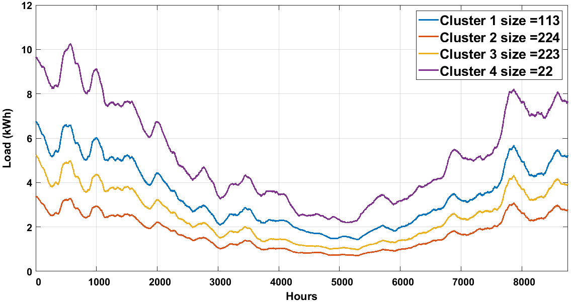
Figure 12: Total hourly loads of different clusters of consumers for one year in Sweden dataset. Figure is best seen in color.

We apply svd on $A$ to get $A=U\Sigma V^{T}$ and consider its approximation $A_{d}:=U_{d}\Sigma_{d}{V_{d}}^{T}$. Let $H:=U_{d}\Sigma_{d}$, then rows of $H$ are the $d$-dimensional representations of hours of $A$. Each column of $H$ is a feature of hours, based on the loads of all consumers in $A$. We cluster the training hours of $H$ into $r$ clusters, ${\mathcal{C}}=\{C_{1},C_{2},\ldots,C_{r}\}$. Each cluster $C_{i}$ contains hours that are substantially similar to each other based on the overall consumption patterns (see Figure 12 in appendix).

We choose the values of $d$ (the number of reduced dimensions) and $r$ (the number of clusters) by evaluating the quality of clusters. The chosen values for $r$ are $80$, $70$, and $70$, while those for $d$ are $300$, $424$, and $34$ for Sweden, Ireland, and Australia datasets respectively.

Remark 2

No dimensionality reduction is applied for the Australia dataset as the number of consumers (columns of the load matrix) is already small, i.e. ”$34$”.

Remark 3

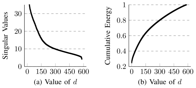
Figure 11: (a) Singular values, and (b) Cumulative energy contained in the first $d$ dimensions of $\Sigma$ (for Sweden dataset).

We selected the singular values $d$ of $\Sigma$ for svd that preserve $80\%$, $80\%$, and $100\%$ cumulative energy in $\Sigma$ for Sweden, Ireland, and Australia datasets, respectively. We can see in Figure 11 (in appendix) that $d=300$ (for $d\leq r$) contains $80\%$ of the cumulative energy of $\Sigma$ for Sweden dataset (Figure 11 (b) in appendix).

We use $k$-means++ algorithm [49] to cluster the rows of $H$. To avoid local minima, we replicate the clustering $1000$ times and select the most accurate partition.

Given a customer $j$, we now find other customers similar to $j$. For this, we first take the transpose of matrix $X$ (to represent customers in rows and hours in columns) and apply svd to reduce the number of columns (hours). However, we perform this task for each month’s hours separately (to capture the seasonality information). To do this, we separate the hours of each month ($\approx 720$ hours for each month), which will give us a separate $\approx n\times 720$ dimensional matrix. On each month’s matrix, we apply svd separately columns (and get $10$ principal components) to reduce its dimensions (we get $n\times 10$ dimensional matrix). Then we concatenate values of all months (all $n\times 10$ matrices together for 12 months) to form a single $n\times 120$ dimensional matrix (where $10\times 12=120$). We refer to this as the seasonal svd approach. The top $k$ similar consumers (rows in this new matrix) to consumer $j$ are then selected using the Euclidean similarity. We use $k=3$, empirically set using standard validation set approach [50]).

III-C Calendar Attributes Based Feature Map

We use rows of $H$ to represent corresponding hours of $A$. To predict a test matrix value $B(i,j)$, the load of consumer $j$ at hour $i$, we identify hours of $A$ (represented by clusters in ${\mathcal{C}}$) that are ‘most similar to the query hour $i$ and report an average of loads of consumer $j$ and that of its top $k$ neighbors in those clusters. The only information of a query hour we can use is its calendar attributes, i.e., time, day, and month. On the other hand, attributes of clusters of training hours (columns of $H$) are based on overall consumption at those hours.

For a common representation of an hour and a cluster of hours, we use a $75$-dimensional vector, $\mathbf{v}(\cdot)$. The first $24$ coordinates of $\mathbf{v}(\cdot)$ ($\mathbf{v}[0\ldots 23]$) correspond to the $24$ hours in a day. The next $7$ coordinates represent the days of a week, and the $31$ coordinates after them represent the days of a month. The following $12$ coordinates stand for the months of a year. The $74^{th}$ and $75^{th}$ coordinates encode public holidays.

For a given hour $h$ (a time-stamp with associated calendar information), the value of $\mathbf{v}(h)$ at a coordinate is $1$ if $h$ has the corresponding attribute. Figure 3(a) depicts an example vector representation of an hour. For a cluster $C=\{h_{1},h_{2},\ldots,h_{|C|}\}$ of hours, $\mathbf{v}(C)$ is the distribution of hours (represented as $\mathbf{v}(\cdot)$) contained in $C$. Formally, $\mathbf{v}(C)=\frac{1}{|C|}\sum_{h\in C}\mathbf{v}(h).$ Figure 3(b) depicts an example vector representation of a cluster of hours (rows of $H$).

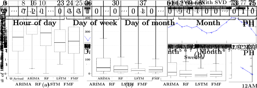
Figure 3: Vector encoding of (a) an hour: Mon $7^{th}$ Jul, 4-5 PM (b) a cluster containing $\mathbf{70\%}$ 8 AM, $\mathbf{20\%}$ 9 AM and $\mathbf{10\%}$ 10 AM hours, half each of Mondays and Tuesdays. $\mathbf{90\%}$ hours are of Jan and $\mathbf{10\%}$ of Feb.

III-D Forecasting the Load

Finally, we describe the mechanism to estimate load of household $j$ at a testing hour $i$, i.e. value of $B(i,j)$. To predict $B(i,j)$, we report an ‘average’ of household $j^{th}$’s load along with the load of its top $k$ neighbors in the clusters of hours in $A$ that are most similar to the query hour $i$. For this, we need a measure of distance/similarity, $d({h},C)$ between a testing hour ${h}$ and a cluster of training hours $C$. Since, the vector representations $\mathbf{v}({h})$ and $\mathbf{v}(C)$ (for hour $h$ and cluster$C$ respectively), encode attributes of $h$ and $C$ related to time, day and month etc. We define $d({h},C)$ to be a weighted sum of the $l_{p}$-distance between the corresponding attributes of ${h}$ and $C$. More precisely, let $d[q]$ be the absolute difference between the $q^{th}$ coordinate of $\mathbf{v}({h})$ and $\mathbf{v}(C)$, i.e. $d[q]=|\mathbf{v}({h})[q]-\mathbf{v}(C)[q]|$. Consider a vector $``\mathbf{w}"$ that contains weights of attributes $w_{1},w_{2},\ldots,w_{8}$. Also consider another vector $``\mathbf{a}"$ that contains following elements of the feature vector related to calendar attributes: $a_{1}=\bigg{(}\sum\limits_{q=0}^{23}(d[q])^{p}\bigg{)}^{\nicefrac{{1}}{{p}}}$, $a_{2}=\bigg{(}\sum\limits_{q=24}^{30}(d[q])^{p}\bigg{)}^{\nicefrac{{1}}{{p}}}$, $a_{3}=\bigg{(}\sum\limits_{q=31}^{61}(d[q])^{p}\bigg{)}^{\nicefrac{{1}}{{p}}}$, $a_{4}=\bigg{(}\sum\limits_{q=62}^{73}(d[q])^{p}\bigg{)}^{\nicefrac{{1}}{{p}}}$,
$a_{5}=\bigg{(}\sum\limits_{q=74}^{75}(d[q])^{p}\bigg{)}^{\nicefrac{{1}}{{p}}}$.

The distance $d(h,C)$ between $h$ and $C$ is defined as $d(h,C):=\mathbf{a^{T}}\mathbf{w}$.

The optimum values for the weights of attributes ($w_{1},w_{2},\ldots,w_{8}$) are computed using the standard validation set approach [50]. The similarity, $sim(h,C)$ between an hour ${h}$ and a cluster $C$ is given by $sim({h},C):=1-d({h},C)$. To predict $B(i,j)$, we find a subset ${\mathcal{C}}^{\prime}\subset{\mathcal{C}}$ of $t$ clusters that have the highest similarity with the hour $i$ and a subset of top $k$ nearest neighbors of consumer $j$ (i.e. $N_{1}(j),\cdots,N_{k}(j)$). We report the similarity-weighted mean of the median consumption of sub-matrix, which consists of loads of consumer $j$, $N_{1}(j),\cdots,N_{k}(j)$ in these $t$ clusters (we empirically select $t=2$ for all datasets). In other words, fmf computes a forecast $B^{\prime}(i,j)$ for the load $B(i,j)$ as follows:

$$B^{\prime}(i,j)=\frac{\sum_{C\in\mathcal{C^{\prime}}}\{sim(i,C)\times\textsc{median}_{h\in C}\cdot\{a\}\}}{\sum_{C\in\mathcal{C^{\prime}}}sim(i,C)}$$ (1)

$$a\;=\;\textsc{median}_{x\in N(j)}A(h,x)$$ (2)

III-E Time Complexity of fmf

The running time of the preprocessing is linear with respect to the size of the input. The training matrix $A$ has dimensions $m_{1}\times n$, svd on $A$ that takes $O(\min(m_{1}n^{2},m_{1}^{2}n))$ time. The next step of the algorithm is clustering training hours. The standard $k$-means algorithm takes time proportional to $O(nrI)$, where $r$ is the number of clusters and $I$ is the number of iterations of the $k$-means algorithm (similar is the case for clustering the customers). Note that these $t$-nearest neighbors are found for each hour only, not for individual consumers, i.e., for every row of $B$, we perform this step only once. Therefore, the total time required for all nearest neighbors computations is $O(m_{2}rt)$. Thus the total running time of all these steps is $O(\min(m_{1}n^{2},m_{1}^{2}n)+nrI+m_{2}rt)$, where $r,t,I$ are user-set parameters and usually small constants. Hence the time complexity is dominated by the svd step. To make a forecast, we compute the medians in each nearest cluster and report an average of these medians. Thus the worst-case runtime of a forecast is $O(m_{1})$.

IV Experimental Setup

In this section, we first describe the three benchmark datasets that we use for evaluating fmf. We then describe the evaluation metrics used to measure the goodness of our approach. We also discuss the baseline and state-of-the-art methods for stlf used for comparison with fmf. In the end, we show the visual representation of data to analyze the hidden patterns (if any exist in the data). Our algorithms are implemented in Matlab and Python on a Core i7 pc with 8GB memory. Code of fmf and the pre-processed datasets are available online for reproducibility.

IV-A Dataset Description and Visualization

We use real-world smart meter data of hourly consumption from different residential areas of Sweden [51, 52, 16], Australia [6] and Ireland [53]. Table I shows detail statistics of these datasets.

Dataset	Households	Hours	Duration	Avg. load	Std. dev.
Sweden	582	17544	Jan 1, 04-Dec 31, 05	2.52	0.81
Ireland	709	12864	Jul 14, 09-Dec 31, 10	1.33	1.33
Australia	34	26304	Jul 1, 10-Jun 30, 13	0.79	0.29

TABLE I: Statistics of datasets: Only the first $12864$ hours ($\approx 18$ months) data is used from all datasets.

To visually examine natural clusters in the data (if any), we embed time-stamps into a $2d$ real vector space using $t$-distributed stochastic neighbor embedding ($t$-sne) [54]. Recall that $X\in\mathbb{R}^{m\times n}$ is the load matrix, where $m$ is the number of hours, and $n$ is the number of households. We apply $t$-sne on the rows of $X$ to get a matrix $F\in\mathbb{R}^{m\times 2}$. We plot the rows of $F$ with each row labeled based on the calendar attributes to observe patterns in the data visually.

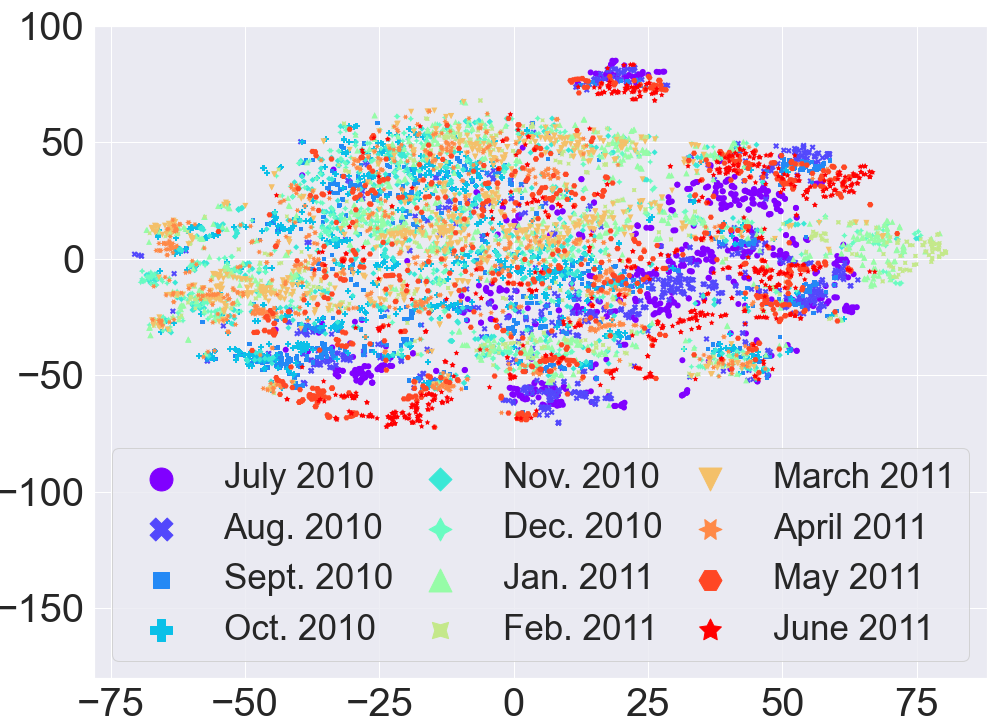
(a) Month wise labels

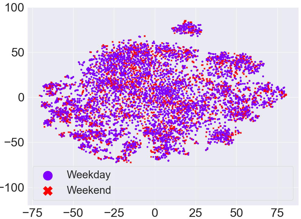
(b) Weekdays/Weekends

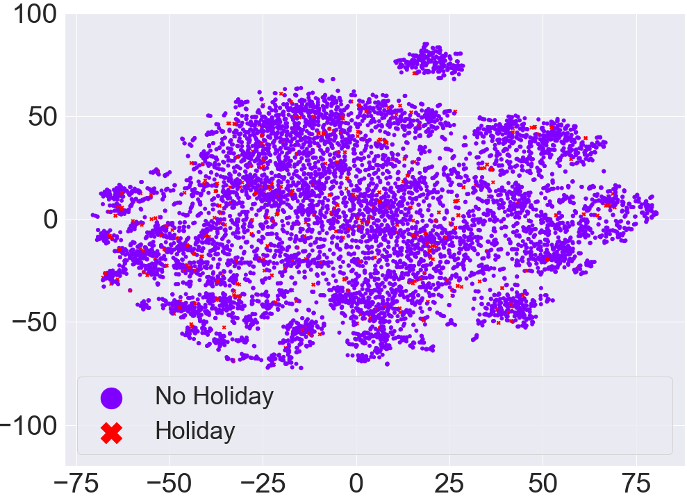
(c) Public Holiday

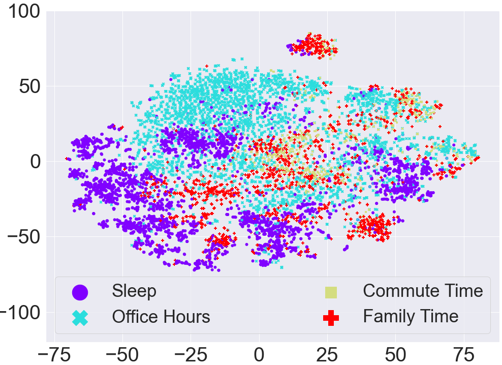
(d) Hours of the Day

Figure 4: The t-sne plots of different labels for Australia dataset. Figure is best seen in color.

Figure 4(a) shows the $t$-sne plot for the Australia dataset with hours assigned month names as labels. Although we can observe some small clusters (i.e., July 2010 and June 2011 at the top center of the plot), there is no clear separation between data points based on months. Similarly, there is no clear separation between hours based on “Weekdays” and “Weekends” or based on “Public Holiday” and “No Public Holiday” (Figure 4(b) and 4(c)). We also group hours of a day into $4$ periods namely “Sleep Time” (12:00 AM – 8:00 AM), “Office Hours” (8:00 AM – 5:00 PM), “Commute Time” (5:00 PM – 7:00 PM), and “Family Time” (7:00 PM – 12:00 AM). We can observe in Figure 4(d) that there are some patterns for sleep hours, office hours, and family time. However, there is no complete separation between different labels. Overall, this scattered behavior shows no clear pattern in the data, i.e., extracting any useful information from data without any preprocessing is not easy.

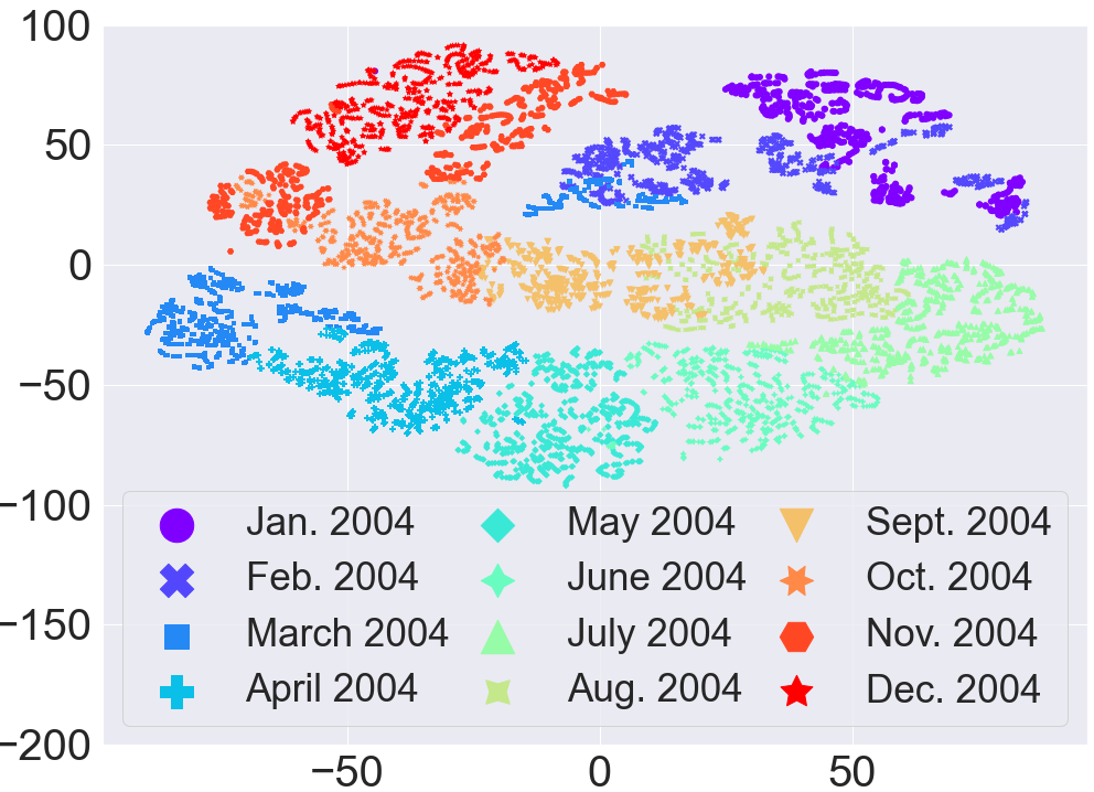
(a) Month wise labels

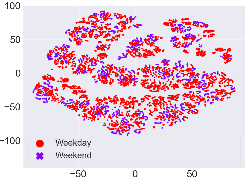
(b) Weekdays/Weekends

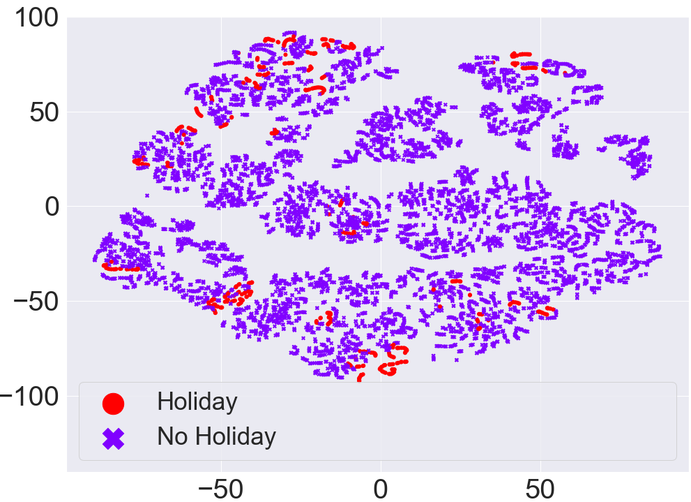
(c) Public Holiday

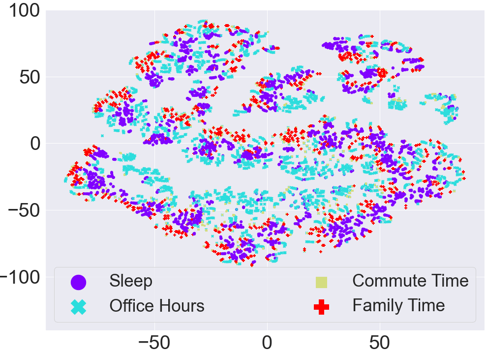
(d) Hours of the Day

Figure 14: The t-sne plots of different labels for Sweden Dataset. Figure is best seen in color.

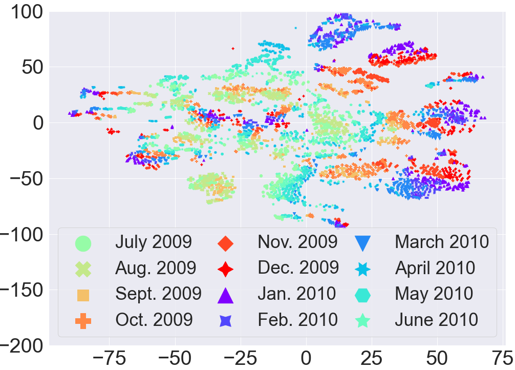
(a) Month wise labels

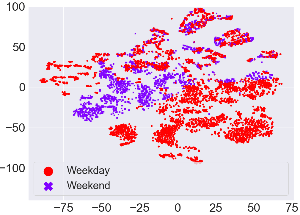
(b) Weekdays/Weekends

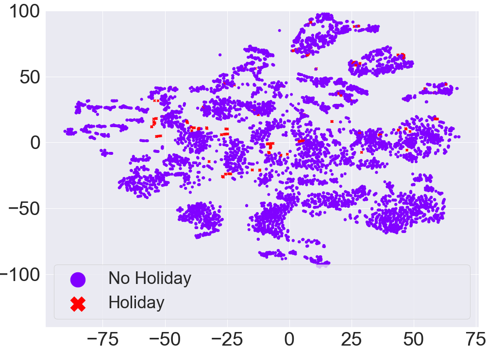
(c) Public Holiday

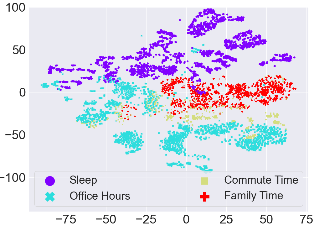
(d) Hours of the Day

Figure 15: The t-sne plots of different labels for Ireland dataset. Figure is best seen in color.

The $t$-sne plots for the Sweden dataset, Figure 14 (in appendix), unlike the Australia dataset, reveal some grouping between months ((Figure 14(a)) and days (weekend/weekdays Figure 14(b)). In the Ireland dataset, we can observe that the weekends and weekdays are clearly grouped (Figure 15(b)). Similarly, the hours of the day in Figure 15(d) show a separation between office hours and sleep hours, but the family time and commute time overlap.

IV-B Evaluation Setup and Metrics

We use the following error metrics to test the performance of fmf: Mean Absolute Error (mae) [10], Mean Absolute Percentage Error (mape) [9], Root Mean Square Error (rmse) [6] and Normalized Root Mean Square Error (nrmse). From all datasets, we use data of first $18$ months in our experiments. Out of these $18$ months data, the first $\approx 12$ months of data ($m_{1}=8760$ (hours)) is used as training data. The succeeding $\approx 6$ months data ($m_{2}=4104$ (hours)) is used for testing.

IV-B1 Clustering Evaluation

We evaluate the effectiveness of clustering hours in the abstract feature-space (rows of $H=U_{d}\Sigma_{d}$) by observing clusters representations, $\mathbf{v}(\cdot)$. We note that hours expected to have similar consumption based on domain knowledge tend to be grouped into the same clusters.

Figure 5: Bar graphs of $\mathbf{v}(\cdot)$ for three clusters of hours (Ireland dataset). All three clusters (a), (b), and (c) shows that similar load pattern hours tend to be in the same clusters.

Figure 5 depicts three randomly chosen clusters and shows that clustering of rows of $H$ is meaningful and successfully avoids the curse of dimensionality. The first cluster (a) contains the winter night hours ($12AM$ to $8AM$) of one whole week. The second cluster (b) is for the daytime summer weekends, while the last cluster (c) is for the evening hours of winter weekends.

Remark 4

Note that we perform clustering only once, and the same clusters are used to predict the entire test matrix $B$ (i.e. $\approx 6$ months hourly load).

Figure 12 (in appendix) shows the clusters of consumers for Sweden dataset. Clusters are well separated in terms of load, highlighting the effectiveness of clustering in our representation. Similar behavior is observed for other datasets.

IV-C Comparison Algorithms

We compare the results of fmf with several baselines and state-of-the-art methods proposed in the literature.

IV-C1 Baseline Method

We use Auto Regressive Integrated Moving Average (arima), a time series model, as a baseline [10]. arima treats historical loads as a time series and attempts to learn parameters for forecasting future values. Our second baseline is ‘Persistent Forecast’, which uses an average of “previous hours” loads as the forecast for the next hour.

IV-C2 State-of-the-Art (sota) Methods

The sota methods that we use for comparison with fmf are the following: Long Short Term Memory (lstm) [9, 20], Multiple Linear Regression (mlr) [6], Regression Trees (rt) [6], Neural Network (nn) [6, 20], Support Vector Regression (svr) [20], and Random Forest (rf) [20]. Further implementation details (including hyperparameters values) are given in the appendix.

We also compare fmf with the methods proposed in [6] and  [20]. In [6], the authors reported household level stlf results on the Australia dataset using four different machine learning algorithms. We apply fmf on the same dataset (with the same train-test split and settings) and report forecasting accuracy (using the same error metrics). In [20], the authors employed four machine learning models to forecast loads for clusters of consumers for the Ireland dataset. We use their method for clustering consumers into clusters and forecast their loads using fmf and compare the forecasting error with the best and recommended method by [20].

V Results and Discussion

In this section, we report forecasting results of fmf perform a comparison with the baseline, and sota approaches. Since fmf works at any level of user-defined granularity both in spatial and time domains, we demonstrate the effectiveness of fmf for predicting aggregated load of clusters of households and total load for the extended periods ranging from a couple of hours to days.

V-A Evaluation of Hourly forecast at Household level

In this section, we use fmf to perform stlf at household level, i.e. we forecast individual entries of the test matrix $B$. Figure 6 shows the boxplots of actual hourly loads (all $m_{2}\times n$ values in $B$) and the hourly loads forecasted using arima, rf, lstm, and fmf. Note that the loads predicted using fmf is closer to the actual loads than all other methods in all datasets.

Figure 6: Actual and forecasted loads of all hours and all households for arima, rf, lstm and fmf. Observe that fmf forecasts are significantly closer to actual loads in all datasets.

Table II shows the comparison of different methods for hourly load prediction with fmf in terms of average error over all households and hours. In this experimental setting, we forecast the hourly load for the next $6$ months. Note that the actual load values in all datasets are very close to $0$ (see Table I), since they represent individual household loads for a short duration (an hour). Thus, a slight prediction error results in a higher percentage error. This is demonstrated by higher mape ($>30\%$) for all methods. However, rmse, nrmse, and mae values in Table II are small, indicating that the predicted loads are close to actual loads (which is also evident from Figure 6).

Method	Dataset	mae (kWh)	rmse (kWh)	nrmse	mape (%)
arima	Sweden	1.55	1.87	10.79	98.5
	Ireland	1.01	1.44	48.50	223.2
	Australia	0.71	0.89	6.79	199.5
rf [20]	Sweden	1.03	1.57	0.018	51.49
	Ireland	1.20	2.06	0.02	354.9
	Australia	0.72	0.98	0.09	234.2
lstm [9]	Sweden	0.79	1.35	0.017	31.85
	Ireland	0.66	1.30	0.015	149.9
	Australia	0.405	0.65	0.06	90.68
fmf	Sweden	0.78	1.24	0.012	37.1
	Ireland	0.60	1.20	0.014	92.9
	Australia	0.401	0.60	0.05	97.4
fmf $(\%)$ improvement over arima	Sweden	$49.67$	$33.68$	$99.9$	$62.3$
	Ireland	$40.59$	$16.66$	$99.9$	$58.3$
	Australia	$43.6$	$32.58$	$99.2$	$51.1$

TABLE II: Per household average errors of all hours for the next $6$ months load forecasting.

Remark 5

Note that we are forecasting hourly load for the next six months. This is still called short term load forecasting as the hourly load is being forecasted. In the case of medium term load forecasting, the “total load” for a few months is forecasted rather than the hourly load.

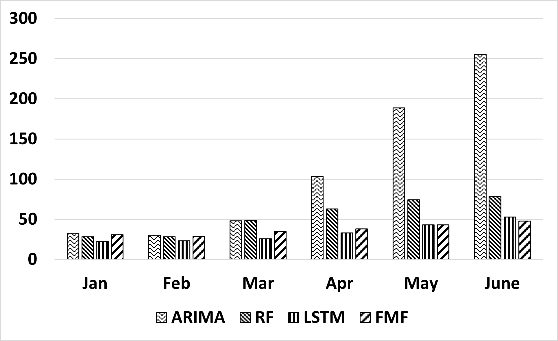
(a)

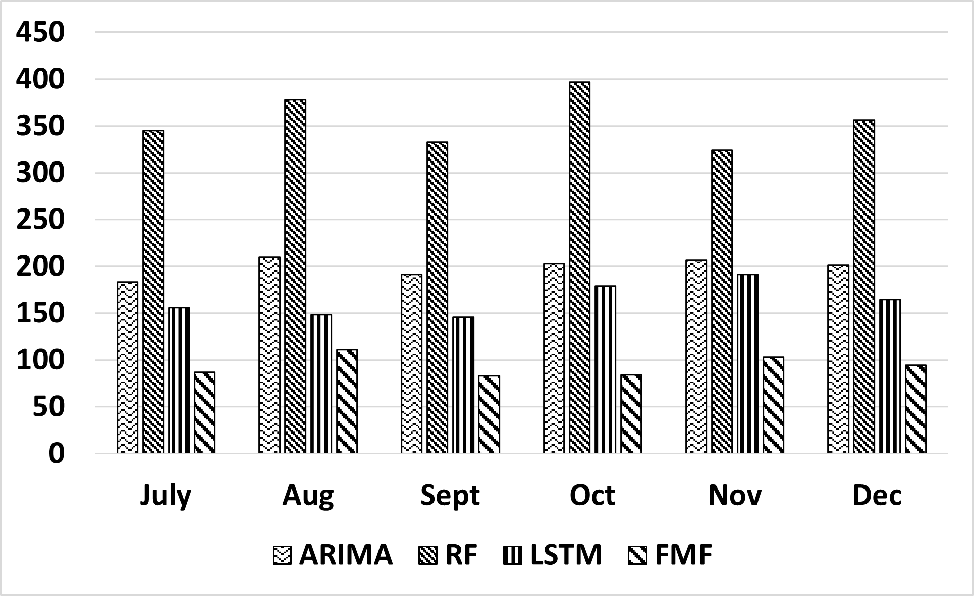
(b)

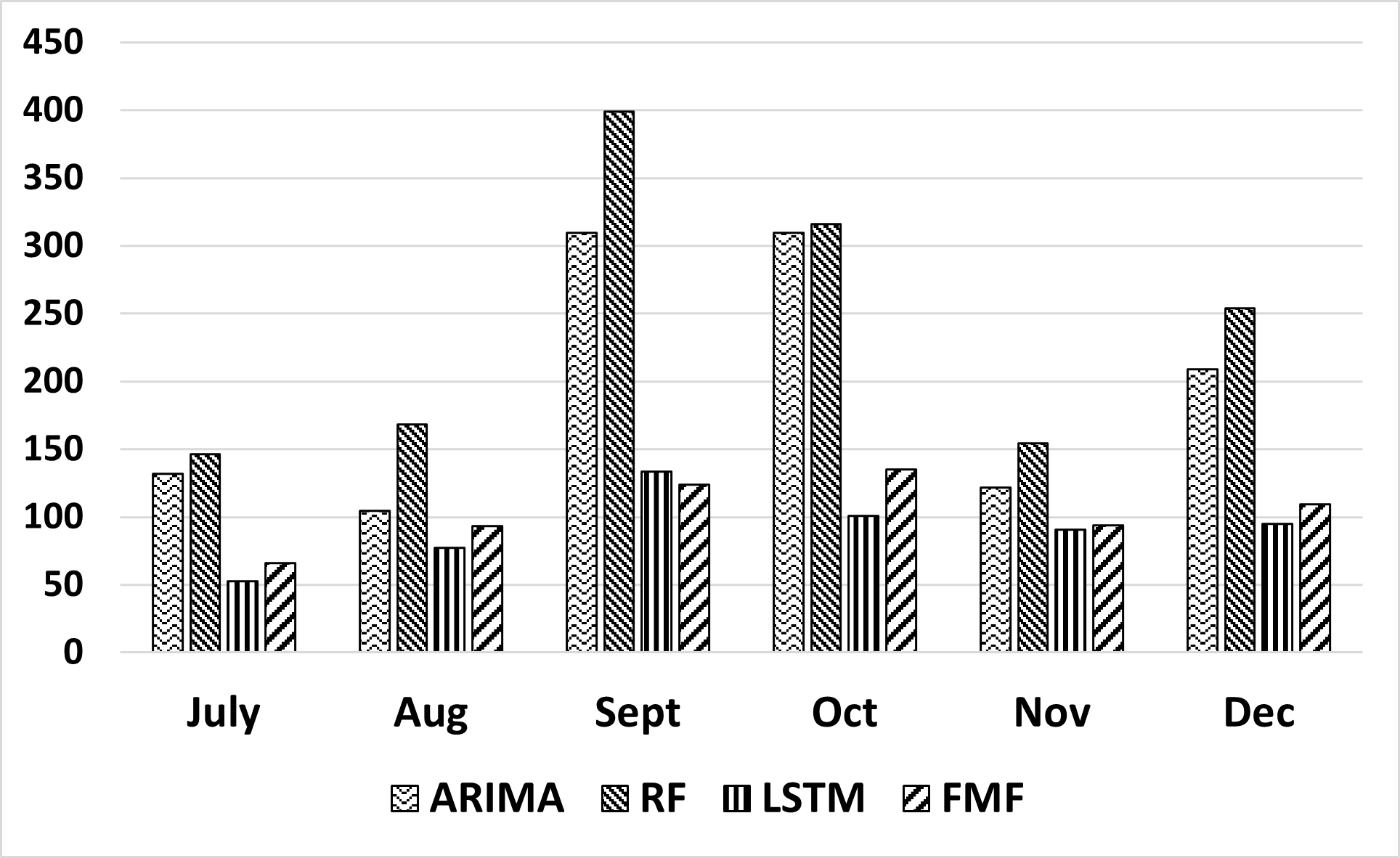
(c)

Figure 7: Monthly mape of arima, rf, lstm and fmf for (a) Sweden (b) Ireland (c) Australia dataset (lower value is better).

Since variability in low loads is relatively much higher, algorithms tend to perform better if the load values of households are on the higher side. Table I shows the average and standard deviation of loads of three datasets. The average load is the largest for the Sweden dataset, and we achieve the minimum mape on it compared to other datasets (see Table II). The average load of households for the Australia dataset is the smallest among the three datasets, and we got a larger mape for this dataset. This also points to the widely accepted phenomenon that forecasting larger aggregated loads is substantially easier than smaller individual loads. We observed in Figure 4, Figure 14 (in appendix), and Figure 15 (in appendix) that the Sweden and Ireland datasets are better separated by different calendar attributes, compared to the Australia dataset. This separability leads to better results on the former two datasets by all error measures.

From Table II it is clear that in most cases, fmf outperforms the baseline and sota approaches. However, these are the mean values of errors, which are very sensitive to outliers. Recall that many actual loads are $0$ or very close to it; there is a sizeable number of outliers in the errors. Therefore, we also plot all point-wise absolute percentage errors in Figure 8 to show that for majority of consumers fmf achieves very low percentage errors. It is clear from Figure 8 that the median percentage error achieved by fmf is the smallest compared to other methods (on the Sweden dataset it is very close to the median performance of lstm).

Figure 8: Absolute percentage errors of all households and all hours for arima, rf, lstm, and fmf.

V-A1 Month-Wise Performance Comparison

To analyze the effect of seasons on forecasting, we report the results for different months. We observe that on the Sweden dataset (Figure 7(a)), fmf is better than all methods for May and June, better than arima and rf for all other months, and comparable to lstm for Jan to April. For the Ireland and Australia dataset (Figure 7(b) and Figure 7(c)), fmf is better than all methods for every month, except in the Australia dataset, it is comparable with lstm.

V-A2 Comparison with Method Proposed in [6]

Authors in [6] perform stlf at even finer granularity ($30$ minutes ahead) using different machine learning methods to perform stlf. For comparison, as performed in [6], we use $28$ days for testing and all remaining data for training “$\approx 2.5$ years” (for Australia dataset). The test data consists of randomly selected weeks in September ($2012$), December ($2012$), March ($2013$), June ($2013$). The comparison, using same parameters, dataset and experimental settings as in [6], is given in Table III. Observe that fmf achieves up to $26.5\%$ improvement in rmse and $94.1\%$ improvement in nrmse.

Method	rmse (kWh)	nrmse
mlr	0.561	2.778
rt	0.516	2.375
svm	0.531	1.793
nn	0.53	2.772
fmf	0.390	0.140
fmf (%) improvement over rt	$24.4$	$94.1$
fmf (%) improvement over svm	$26.5$	$92.1$

TABLE III: Comparison of fmf with different machine learning methods employed by [6] for Australia dataset.

V-A3 Comparison with Persistent Forecast and Autocorrelation Analysis

We designed two settings for the persistent forecast (pf) model and compared them with the fmf results. In the first setting, pf₁, given a query hour $t$, we take the load values for $t-1$, $t-2$ hours of the same day, and $t$ and $t-1$ hours of the previous day and take the average of all these load values as the predicted value. In the second setting, pf₂, given a query hour $t$, we take the load values for $t-1$, $t-2$ hours of the same day, $t$ and $t-1$ hours of the previous day, and $t$ and $t-1$ hours of the same day of the previous week and take the average of all these load values as the predicted value. The result comparison for the pf with fmf are shown in Table IV. A limitation of pf is that it can only be used to forecast the load for the next hour and cannot forecast the hourly load for multiple hours in advance (e.g., hourly load for the next six months or long-term load (e.g., the aggregated load of a month or year).

Dataset	Method	rmse (kWh)	nrmse	mape (%)
Australia	pf1	0.34	0.15	55.53
	pf2	0.46	0.20	65.83
	fmf	0.33	0.14	117.81
Sweden	pf1	0.99	0.037	30.17
	pf2	1.01	0.038	31.57
	fmf	0.95	0.035	26.15
Ireland	pf1	0.68	0.041	102.61
	pf2	0.59	0.036	99.42
	fmf	0.58	0.034	64.23

TABLE IV: Forecasting errors of pf₁, pf₂, and fmf.

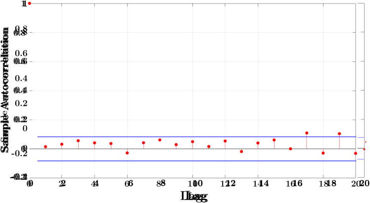
(b) Sweden dataset

Figure 16: Autocorrelation in the datasets. Sweden data has very low autocorrelation for all lag values (similarly Ireland data). The Australia data shows a slightly more significant autocorrelation.

We use autocorrelation to measure the linear relationship between lagged values. We consider lag values (time gap) ranging from $1$ to $20$. A lag $k$ autocorrelation is the correlation between values that are $k$ periods apart. There is a very low average autocorrelation with a small standard deviation in the Sweden dataset (Figure 16(b) in appendix). These values are relative larger in the Australia dataset (Figure 16(a) in appendix). The Ireland dataset has autocorrelation on the lower end too. This explains why pf results on the Australia data are better than the Sweden dataset, hence using more lag values would not increase the forecasting accuracy of pf.

V-A4 Effectiveness of svd

We showed the effectiveness of svd in preserving the original structure of data and making clear clusters of hours (see Section IV-A). Now we report mape for fmf with and without using svd. We observe that svd helps improve the forecasting error for all datasets.

Method	Australia	Sweden	Ireland
fmf without svd	104.79	38.85	103.81
fmf with svd	97.4	37.1	92.9

TABLE V: mape (for the hourly forecast of 6 months) for fmf with and without using svd for hours representation.

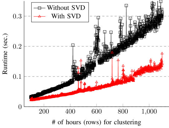
Figure 13: Runtime of $k$-means algorithm ($k=80$) on load matrix without and with dimensionality reduction. Horizontal axis shows the increasing number of hours in the training set.

Moreover, svd also helps reduce the computational runtime of the underlying clustering algorithm (by reducing the dimensionality of the data). We report the effect of dimensionality reduction on the running time of clustering $m$ hours. Recall that each hour is an $n$-d vector ($n=709$, the number of households in the Ireland dataset). Figure 13 (in appendix) plots the runtimes clustering varying number of hours through $k$-means algorithm ($k=80$), when dimensionality of hours is $709$ and $424$ (approximately $80\%$ energy in the singular values is preserved, see Section III-B).

V-B Evaluation of fmf at Higher Granularity

As discussed above, load forecasting at coarser levels (either in space or time dimensions) is substantially easier. This, however, is an important problem in the power sector decision-making. fmf is most suited for stlf at the individual household level, but it is a general-purpose method that works at any level of user-defined granularity and yields significantly more accurate forecasts in most cases. In this section, we use fmf to forecast load for longer durations (up to a day), for groups (clusters) of households, and both combined.

V-B1 Forecast for longer durations

In this section, we show results of fmf and other methods on forecasting loads of individual consumers for longer periods. We add consecutive hours (rows) of the original load matrix in this setting. We aggregated $2,4,12,$ and $24$ consecutive hours of the original load matrix (training and testing data before transformation). Figure 9 shows the mape of fmf, lstm, rf, and arima with increasing hours aggregation. Clearly, with no hour aggregation (when $x$-axis value is $1$), fmf is better than rf and arima on all datasets. fmf yields better results than lstm on the Ireland, comparable on the Sweden and performs slightly worse on the Australia dataset. However, performance of lstm degrades with increasing hours aggregation.

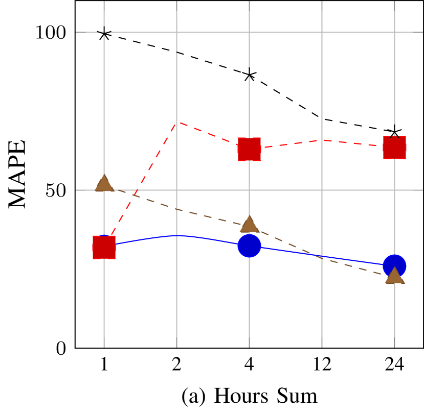
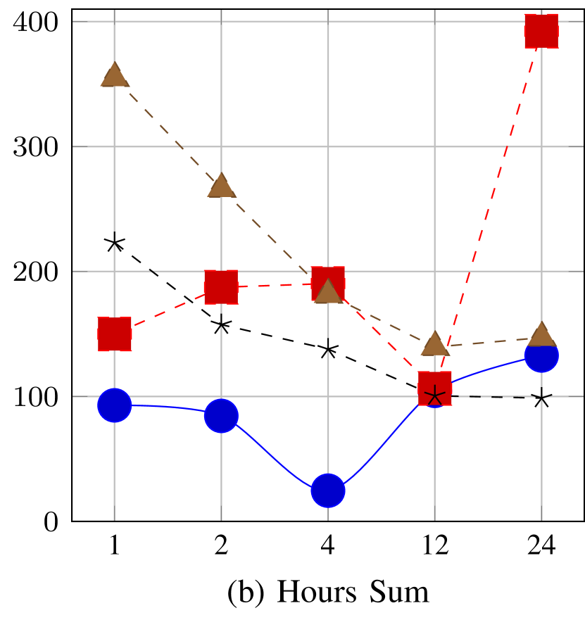
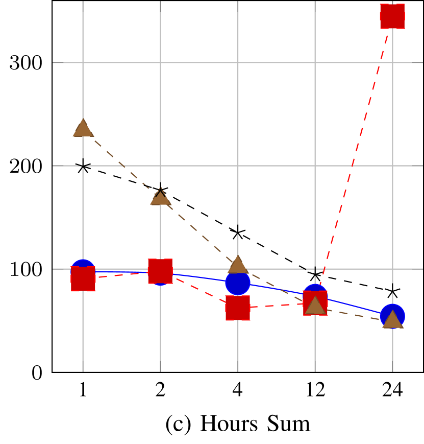
Figure 9: mape comparison of fmf, lstm, rf, and arima with increasing hours aggregation for (a) Sweden, (b) Ireland, and (c) Australia dataset. Figure is best seen in color.

V-B2 Forecast for clusters of households

To evaluate the performance of fmf on higher spatial granularity, we group the households into clusters and forecast the total load of each cluster for individual hours. To compare our fmf with [20], we follow the same train-validation-test split setting ($9$ months-$3$ months-$6$ months) for the Ireland dataset (as used in [20]). We cluster households, represented by our feature vectors (see Section III-B) into varying numbers of clusters ($2$ to $7$). Table VI shows the mape of fmf and the scheme presented in [20]. fmf outperform other methods in majority of the scenarios. We report improvement over rf, the top performing and recommended method in [20].

Techniques	mape for different numbers of clusters
	$2$	$3$	$4$	$5$	$6$	$7$
nn	6	5.3	5	5.1	5	5.2
svr	6	5.3	5.1	5.1	5.2	5.4
rf	6.1	5	4.6	4.6	4.7	4.7
lstm	10.8	9.2	9	8.5	8.7	8.6
fmf	4.4	3.2	4.8	4.3	4.3	5.6
%-improvement of fmf over rf	$22.8$	$36$	$-4.3$	$6.5$	$8.5$	$-19.1$

TABLE VI: mape of fmf and models proposed in [20] on the Ireland dataset with increasing number of household clusters.

V-B3 Forecast of clusters of households for longer durations

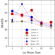
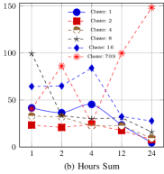
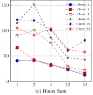
Figure 17: mape of fmf for groups of households and longer durations. ‘Cluster: $i\,$’ means households are grouped into $i$ clusters. Datasets: (a) Sweden (b) Ireland (c) Australia

In this section, we first aggregate hours (add consecutive hours) and then households (cluster the households and aggregate their total loads) and then forecast the total load using fmf. We report the errors in clusters’ total forecasted loads for different periods (consecutive hours sum shown on the horizontal axis) for varying numbers of clusters. We can see from Figure 17 (in appendix) that forecasting the aggregated load (both row “hours” and column “households” wise) helps to reduce the error in most cases. The error values show some variations, but overall the error reduces as we aggregate the hours and households. The spikes in some cases are due to randomness in loads of households.

VI Conclusion and Future Work

Short-term load forecasting is a fundamental task in power system operations. stlf at the household level is pivotal for demand response programs such as peak shaving, dynamic pricing, and soft load shedding. In this work, we proposed a matrix factorization-based method called fmf for short-term load forecasting at the individual consumer level. fmf is computationally less expensive and can be applied to any locality because it does not use any consumers’ demographic or activity pattern data. fmf forecast the hourly load of individual households with high accuracy compared to state-of-the-art machine learning-based methods e.g. lstm, svm, rf etc. We have observed up to $49\%$ improvement in mae, up to $33\%$ improvement in rmse, up to $99\%$ improvement in nrmse and up to $62\%$ improvement in mape over other techniques for stlf on different datasets. fmf also produce promising results on forecasting loads of clusters of consumers for longer durations. This illustrates the general ability of fmf to apply in any temporal and spatial granularity. Potential future work is to combine fmf with existing machine learning methods in an ensemble-based approach. Another future direction is to extend the approach of fmf to the problems of wind speed and solar intensity forecasting.

Appendix A Implementation Details

A separate model is learned for each household by arima and rf while a single model is learned for all households by lstm due to its computational complexity.

A-1 arima

The input parameters for arima are the maximum and minimum number of autoregressive terms ($p$), the maximum and the minimum number of nonseasonal differences needed for stationarity ($q$), and the maximum and minimum number of lagged forecast errors ($d$). The output is an arima model fitted according to Akaike Information Criterion. We select $d=0$, minimum $p=1$, maximum $p=5$, minimum $q=1$, maximum $q=5$. We fit Seasonal arima (sarima), which is more suitable due to capturing seasonal information, sarima $(p,q,d)(P,Q,D,S)$. The value of $S$ is $24$ because of seasonality effect. Maximum $P$ and maximum $Q$ values are taken as $2$, and maximum $D$ value is taken as $0$.

A-2 Random Forest (rf)

Two essential hyperparameters for rf are ’maximum number of attributes used in a tree’ and the ’the number of trees’, which are tuned using a validation set. As we increase the number of trees the error decreases, as shown in Figure 10(b). Due to computational constraints, we select $100$ trees, and the maximum attributes used in each decision tree are $29$. This attributes count is chosen using grid search on the validation set with (mse) as error metric. In Figure 10 (a), mse has least value against the attribute count of $29$. Since rf is invariant to scaling, we used Table VII features without scaling. A separate model is learned (with different hyperparameters) for each consumer in each dataset.

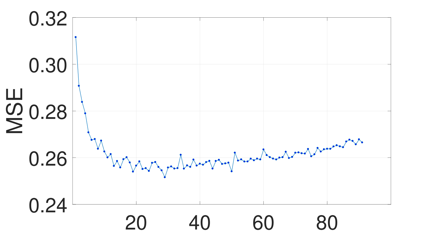
(a) Attributes for Individual Tree

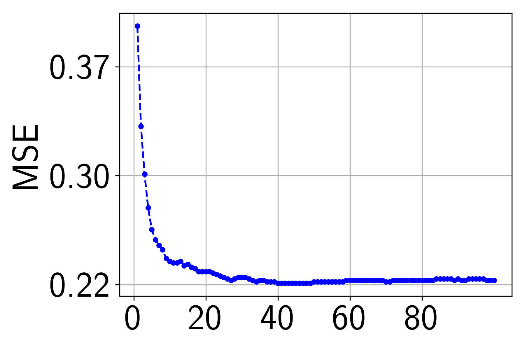
(b) Total Number of Trees

Figure 10: Hyperparameter tuning of Random Forest for a single Household of Sweden dataset.

A-3 lstm

The architecture of lstm scheme proposed in [9] consists of $2$ hidden layers with $20$ nodes in each layer. A simple neural network with sigmoid activation function is used to ensemble the final prediction. The features used in lstm are shown in Table VII. The number of previous time-stamps used in the forecasting is $6$. Furthermore, mse with Adam optimizer [55] is used to perform training for $100$ epochs. Since lstm contains a large number of weights, learning these weights requires huge amount of data. We test separate lstm models for each consumer and a single model on all consumers. Due to less amount of data, a separate model on individual consumer performs poorly compared to a single model for all consumers. Therefore, we only include the results of a single model for all consumers in each dataset.

Index	Variable	Description
1-24	Hours	One hot encoding vector
25-31	Day of Week	One hot encoding vector
32-62	Day of Month	One hot encoding vector
63-74	Month	One hot encoding vector
75-85	Lagged Input	3 previous hours of same day, 4 hours of previous day including predicted hour predicted, 4 hours of same day previous week
86	Public Holiday	Boolean input
87	Temperature	Single numeric input
88	Wind Speed	Single numeric input
89	Humidity	Single numeric input

TABLE VII: Input parameters for the classification algorithms.

Appendix B Supplementary Results

(a) Australia dataset

References

- [1] T. Hong and S. Fan, “Probabilistic electric load forecasting: A tutorial review,” International Journal of Forecasting, vol. 32, pp. 914–938, 2016.
- [2] X. Qiu, P. Suganthan, and G. Amaratunga, “Ensemble incremental learning random vector functional link network for short-term electric load forecasting,” Knowledge Based Systems, vol. 145, pp. 182–196, 2018.
- [3] Y. Wang, Y. Shen, S. Mao, X. Chen, and H. Zou, “Lasso and lstm integrated temporal model for short-term solar intensity forecasting,” IEEE Internet of Things Journal, vol. 6, pp. 2933–2944, 2018.
- [4] W. Wu and M. Peng, “A data mining approach combining -means clustering with bagging neural network for short-term wind power forecasting,” IEEE Internet of Things Journal, vol. 4, pp. 979–986, 2017.
- [5] M. Malekizadeh, H. Karami, M. Karimi, A. Moshari, and M. Sanjari, “Short-term load forecast using ensemble neuro-fuzzy model,” Energy, vol. 196, p. 117127, 2020.
- [6] P. Lusis, K. Khalilpour, L. Andrew, and A. Liebman, “Short-term residential load forecasting: Impact of calendar effects and forecast granularity,” Applied Energy, vol. 205, pp. 654–669, 2017.
- [7] U. Amato, A. Antoniadis, I. Feis, Y. Goude, and A. Lagache, “Forecasting high resolution electricity demand data with additive models including smooth and jagged components,” International Journal of Forecasting, vol. 37, pp. 171–185, 2021.
- [8] I. Koprinska, M. Rana, and V. Agelidis, “Correlation and instance based feature selection for electricity load forecasting,” Knowledge Based Systems, vol. 82, pp. 29–40, 2015.
- [9] W. Kong, Z. Dong, Y. Jia, D. Hill, Y. Xu, and Y. Zhang, “Short-term residential load forecasting based on lstm recurrent neural network,” IEEE Transactions on Smart Grid, vol. 10, pp. 841–851, 2019.
- [10] H. Shi, M. Xu, and R. Li, “Deep learning for household load forecasting—a novel pooling deep rnn,” IEEE Transactions on Smart Grid, vol. 9, pp. 5271–5280, 2018.
- [11] J. Ping, L. Feng, and S. Yiliao, “A hybrid forecasting model based on date-framework strategy and improved feature selection technology for short-term load forecasting,” Energy, vol. 119, pp. 694–709, 2017.
- [12] N. Amjady and F. Keynia, “Short-term load forecasting of power systems by combination of wavelet transform and neuro-evolutionary algorithm,” Energy, vol. 34, pp. 46 – 57, 2009.
- [13] S. Haben, J. Ward, D. Greetham, C. Singleton, and P. Grindrod, “A new error measure for forecasts of household-level, high resolution electrical energy consumption,” International Journal of Forecasting, vol. 30, pp. 246–256, 2014.
- [14] M. Felice and X. Yao, “Short-term load forecasting with neural network ensembles: A comparative study [application notes],” IEEE Computational Intelligence Magazine, vol. 6, pp. 47–56, 2011.
- [15] T. Aslam and N. Arshad, “Soft load shedding: An efficient approach to manage electricity demand in a renewable rich distribution system,” in International Conference on Smart Cities and Green Systems, 2018, pp. 101–107.
- [16] S. Ali, H. Mansoor, I. Khan, and N. Arshad, “Fair allocation based soft load shedding,” in Intelligent Systems Conference, 2020, pp. 1–17.
- [17] “The United States of America, Department of Energy,” 7 March, 2022. [Online]. Available: www.energy.gov/energysaver/articles/modern-smart-meters-offer-consumers-power-choice
- [18] K. Gajowniczek and T. Zabkowski, “Electricity forecasting on the individual household level enhanced based on activity patterns,” PlOS ONE, vol. 12, 2017.
- [19] Y. Hsiao, “Household electricity demand forecast based on context information and user daily schedule analysis from meter data,” IEEE Transaction on Industrial Informatics, vol. 11, pp. 33–43, 2015.
- [20] A. Kell, A. McGough, and M. Forshaw, “Segmenting residential smart meter data for short-term load forecasting,” in International Conference on Future Energy Systems, 2018, pp. 91–96.
- [21] F. Quilumba, W. Lee, H. Huang, D. Wang, and R. Szabados, “Using smart meter data to improve the accuracy of intraday load forecasting considering customer behavior similarities,” IEEE Transaction on Smart Grid, vol. 6, pp. 911–918, 2015.
- [22] H. Li, Y. Zhao, Z. Zhang, and X. Hu, “Short-term load forecasting based on the grid method and the time series fuzzy load forecasting method,” in International Conference on Renewable Power Generation, 2015, pp. 1–6.
- [23] R. Zhang, Y. Xu, Z. Dong, W. Kong, and K. Wong, “A composite k-nearest neighbor model for day-ahead load forecasting with limited temperature forecasts,” in IEEE Power and Energy Society General Meeting, 2016, pp. 1–5.
- [24] M. Ghofrani, M. Ghayekhloo, A. Arabali, and A. Ghayekhloo, “A hybrid short-term load forecasting with a new input selection framework,” Energy, vol. 81, pp. 777–786, 2015.
- [25] J. Taylor, “An evaluation of methods for very short-term load forecasting using minute-by-minute british data,” International Journal of Forecasting, vol. 24, pp. 645–658, 2008.
- [26] Y. Chakhchoukh, P. Panciatici, and L. Mili, “Electric load forecasting based on statistical robust methods,” IEEE Transactions on Power Systems, vol. 26, pp. 982–991, 2011.
- [27] J. Che and J. Wang, “Short-term load forecasting using a kernel-based support vector regression combination model,” Applied energy, vol. 132, pp. 602–609, 2014.
- [28] H. Saxena, O. Aponte, and K. McConky, “A hybrid machine learning model for forecasting a billing period’s peak electric load days,” International Journal of Forecasting, vol. 35, pp. 1288–1303, 2019.
- [29] S. Li, L. Goel, and P. Wang, “An ensemble approach for short-term load forecasting by extreme learning machine,” Applied Energy, vol. 170, pp. 22–29, 2016.
- [30] U. Tayab, A. Zia, F. Yang, J. Lu, and M. Kashif, “Short-term load forecasting for microgrid energy management system using hybrid hho-fnn model with best-basis stationary wavelet packet transform,” Energy, p. 117857, 2020.
- [31] A. Yang, W. Li, and X. Yang, “Short-term electricity load forecasting based on feature selection and least squares support vector machines,” Knowledge Based Systems, vol. 163, pp. 159–173, 2019.
- [32] Z. Liao, H. Pan, X. Fan, Y. Zhang, and L. Kuang, “Multiple wavelet convolutional neural network for short-term load forecasting,” IEEE Internet of Things Journal, vol. 8, pp. 9730–9739, 2020.
- [33] M. A. Zamee, D. Han, and D. Won, “Online hour ahead load forecasting using appropriate time-delay neural network based on multiple correlation-multicollinearity analysis in iot energy network,” IEEE Internet of Things Journal, pp. 1–1, 2021.
- [34] B. Stephen, X. Tang, P. Harvey, S. Galloway, and K. Jennett, “Incorporating practice theory in sub-profile models for short term aggregated residential load forecasting,” IEEE Transactions on Smart Grid, vol. 8, pp. 1591–1598, 2017.
- [35] S. Ryu, J. Noh, and H. Kim, “Deep neural network based demand side short term load forecasting,” Energies, vol. 10, p. 3, 2017.
- [36] X. Dong, L. Qian, and L. Huang, “Short-term load forecasting in smart grid: A combined cnn and k-means clustering approach,” in International Conference on Big Data and Smart Computing, 2017, pp. 119–125.
- [37] R. Li, F. Li, and N. Smith, “Multi-resolution load profile clustering for smart metering data,” IEEE Transactions on Power Systems, vol. 31, pp. 4473–4482, 2016.
- [38] P. Silva, D. Ilic, and S. Karnouskos, “The impact of smart grid prosumer grouping on forecasting accuracy and its benefits for local electricity market trading,” IEEE Transactions on Smart Grid, vol. 5, pp. 402–410, 2013.
- [39] K. Gajowniczek and T. Zabkowski, “Short term electricity forecasting using individual smart meter data,” Procedia Computer Science, vol. 35, pp. 589–597, 2014.
- [40] M. Ghofrani, M. Hassanzadeh, M. Etezadi, and M. Fadali, “Smart meter based short-term load forecasting for residential customers,” in North American Power Symposium, 2011, pp. 1–5.
- [41] P. Athukorala and C. Wilson, “Estimating short and long-term residential demand for electricity: New evidence from sri lanka,” Energy Economics, vol. 32, pp. S34–S40, 2010.
- [42] A. Veit, C. Goebel, R. Tidke, C. Doblander, and H. Jacobsen, “Household electricity demand forecasting: benchmarking state-of-the-art methods,” in International Conference on Future Energy Systems, 2014, pp. 233–234.
- [43] D. Ignatiadis, G. Henri, and R. Rajagopal, “Forecasting residential monthly electricity consumption using smart meter data,” in North American Power Symposium, 2019, pp. 1–6.
- [44] E. Mocanu, P. Nguyen, M. Gibescu, and W. Kling, “Deep learning for estimating building energy consumption,” Sustainable Energy, Grids and Networks, vol. 6, pp. 91–99, 2016.
- [45] B. Yildiz, J. Bilbao, J. Dore, and A. Sproul, “Household electricity load forecasting using historical smart meter data with clustering and classification techniques,” in IEEE Innovative Smart Grid Technologies Asia, 2018, pp. 873–879.
- [46] M. Chaouch, “Clustering-based improvement of nonparametric functional time series forecasting: Application to intra-day household-level load curves,” IEEE Transactions on Smart Grid, vol. 5, pp. 411–419, 2013.
- [47] A. Singh, Ibraheem, S. Khatoon, M. Muazzam, and D. Chaturvedi, “Load forecasting techniques and methodologies: A review,” in International Conference on Power, Control and Embedded Systems, 2012, pp. 1–10.
- [48] G. Strang, Linear algebra and its applications. Belmont, CA: Thomson, Brooks/Cole, 2006.
- [49] D. Arthur and S. Vassilvitskii, “k-means++: The advantages of careful seeding,” in Symposium on Discrete algorithms, 2007, pp. 1027–1035.
- [50] P. Devijver and J. Kittler, “Pattern recognition: A statistical approach.” London, GB: Prentice-Hall, 1982.
- [51] F. Javed, N. Arshad, F. Wallin, I. Vassileva, and E. Dahlquist, “Forecasting for demand response in smart grids: An analysis on use of anthropologic and structural data and short term multiple loads forecasting,” Applied Energy, vol. 96, pp. 150–160, 2012.
- [52] S. Ali, H. Mansoor, N. Arshad, and I. Khan, “Short term load forecasting using smart meter data,” in International Conference on Future Energy Systems, 2019, pp. 419–421.
- [53] “Commission for energy regulation smart metering project - electricity customer behaviour trail, 2009-2010,” 2012. [Online]. Available: www.ucd.ie/issda/data/commissionforenergyregulationcer
- [54] L. Maaten and G. Hinton, “Visualizing data using t-sne.” Journal of Machine Learning Research, vol. 9, pp. 2579–2605, 2008.
- [55] D. Kingma and J. Ba, “Adam: A method for stochastic optimization,” in International Conference on Learning Representations, 2015.