About the Power Spectrum Of Primordial Gravitational Waves

Abstract

The primordial gravitational waves (PGW) have been generated by inflationary amplification of the primordial (quantum) fluctuations. It is true that they have not been recorded directly so far, but their spectrum can help a lot in solving the basic puzzles of the early universe as Inflation (high) energy scale. In the present work, we give a straightforward method to calculate the spectral energy density (SED) of the relic gravitons different from that used in e. g.  [3, 7, 8]. In our approach, the evolution equations are in terms of the scale factor (instead of conformal time) through the Lagrange formalism (instead of the transfer function). The presence of the Hubble parameter allows to calculate the power spectrum in the different dynamical regimes.

Keywords: Gravitational waves; Hubble Parameter; Power Spectrum.

1 Introduction

The gravitational waves (GW) are spacetime curvature disturbances which propagate at speed of light. One of the familiar sources is rapidly accelerated massive objects which make ripples in their surrounding spacetime. These waves were first predicated by Einstein as approximative solutions of the field equations of General Relativity in 1916 [1]. In recent decades, study of GW becomes an interesting topic in theoretical and experimental physics such as GW produced during inflationary period or the compact binary system [2, 3]. The first direct detections of GW was from the merging of black holes and neutron stars reported by the LIGO/VIRGO [4, 5, 6].
GW can give information from regions of spacetime of universe that are not accessible by other source of information as electromagnetic radiation. From the cosmological standpoint, the GW play a potential role to extract or infer the information about theories as Cosmic Inflation. This is due to the tensorial nature of GW, because some information cannot be extracted from the scalar perturbations.
In this work, we are interested in studying and analysing the GW originating in the early universe. To understand and describe of its physical conditions of the early universe, the inflationary paradigm is a very successful theory. This theory was welcomed due to solving the major cosmological problems, because it is well–supported by observational data such as Large Scale Structure of the present universe (this theory is well–described by the scalar perturbations). On the other hand, the tensorial perturbations predict the existence of a uniform background of gravitational radiation in the universe. Despite the very low intensity of GW, observational evidences and technological tools have succeeded in detecting them, the hopes for future are that, by improved technologies one should be able to test the prediction from inflation which this would be a huge success in confirming the theory.
During the inflationary epoch, the other possible physical processes and matter–field fluctuations are also involved in the generation of GW and can be considered as sources of the wave production. These processes can cause the noise in the wave propagation which makes a random character for the GW (what is known as stochastic background GW). The study and investigation of such a background can help us to understand and explore the early universe events and high–energy physics. In fact, the energy scale for which the inflation can occur is one of the main challenge for theoretical and experimental physics and in this way the GW generated at that time can play an important role to probe the such energy scale. In fact, it is believed that since there are no gravitational waves found at the 5 percent level, thus the energy scale of an inflationary epoch was below the Planck scale.
In general case when one deals with a stochastic (radiation) signal, the signal hasn’t a meaningful phase data information (due to the random noise effects) and it is common to use the spectral methods. The spectral energy density (SED)is an important quantity in analysis of the (periodic) signals to extract information. It identifies at what frequency (or frequencies) is the signal power or, what form does the energy density function over frequency have?. Therefore, to study and analysis of the primordial GW, the power spectrum can be used as an useful tool for extracting the information which can not be read from the time domain of the wave. Indeed, these information (as magnitudes of the frequencies components) can be directly related to the energy scale of inflation.
In the present article, we deal with the tensorial perturbations amplified by inflation leading to primordial GW, by special focus on their power spectrum. We calculate the spectral energy in a different way from the one used in the previous works, e. g.  [3, 7, 8]. SED is obtained directly in terms of scale factor, from the beginning of the universe until the present age. In the mentioned works, the spectrum is obtained for each dynamical regime of the universe (that is radiation, matter–radiation and matter regimes) individually and then patch them together. The corresponding spectrum diagrams are also plotted which through them some physics are deduced.
The work is organized as follows:

In section 2, we obtain the wave equation governing the perturbations in terms of the scale factor using the Lagrangian formalism. In section 3, the power spectrum of gravitational waves and corresponding diagrams are presented. Conclusions are given in section 4.

2 Perturbations in FRW Background

In the beginning of this section, let’s give a brief overview of the time evolution of gravitational perturbations, needed for the work. Consider a perturbed FRW spacetime whose line element can be written in the form [3, 7]

$$ds^{2}=g_{\mu\nu}dx^{\mu}dx^{\nu}=\left(\bar{g}_{\mu\nu}+h_{\mu\nu}\right)dx^{\mu}dx^{\nu}=a^{2}\left\{-d\tau^{2}+\left[\delta_{ij}+h_{ij}(t,x)\right]dx^{i}dx^{j}\right\}$$ (1)

where $\tau$ is the conformal time, $\bar{g}_{\mu\nu}=diag\{-a^{2},a^{2},a^{2},a^{2}\}$ is the unperturbed FRW background metric and $h_{\mu\nu}=h_{\mu\nu}(x)$ are the perturbations satisfying $|h_{\mu\nu}|<<1$,  $h_{00}=h_{0i}=0$ and traceless ($h^{i}_{i}=0)$ and transverse $(h^{j}_{i,j}=0)$ conditions. The linearization of Einstein equations (in presence of an isotropic and perfect fluid) for the spectrum of perturbations lead to the following equation [3, 8]:

$$h^{{}^{\prime\prime}}_{k}+2\left(\frac{a^{{}^{\prime}}}{a}\right)h^{{}^{\prime}}_{k}+k^{2}h_{k}=0,$$ (2)

where $h_{k}=h(\tau,k)=\int d^{3}\textbf{x}e^{-i\textbf{k}\cdot\textbf{x}}h(\tau,\textbf{x})$ is the Fourier transform of perturbations and prime denotes derivative with respect to the conformal time $\tau$. For later purposes, we obtain equation (2) by the Lagrangian formalism in the following discussion. The gravitational action describing the tensor perturbations is given by[7]:

$$S=\int d\tau d\textbf{x}\sqrt{-\bar{g}}\left(R+\frac{1}{2}\Pi_{ij}h_{ij}\right)=\int d\tau d\textbf{x}\sqrt{-\bar{g}}\left(\frac{-\bar{g}^{\mu\nu}}{64\pi G}\partial_{\mu}h_{ij}\partial_{\nu}h_{ij}+\frac{1}{2}\Pi_{ij}h_{ij}\right),$$ (3)

where $R$ is the Ricci scalar, $\Pi_{ij}$ is the anisotropic stress tensor and $\bar{g}$ is the determinant of $\bar{g}_{\mu\nu}$. For an isotropic and perfect fluid ($h_{ij}(x)=h(x)$ and $\Pi_{ij}=0\hskip 5.69054pt\cite[cite]{[\@@bibref{}{Steven 2003}{}{}]}$), the action (3) reduces to

$$S=\int d\tau d\textbf{x}\sqrt{-\bar{g}}\left(\frac{\bar{-g^{\mu\nu}}}{64\pi G}\partial_{\mu}h\partial_{\nu}h\right)=\int d\tau d\textbf{x}\mathcal{L},$$ (4)

which gives the Lagrangian as

$$\mathcal{L}=\frac{\bar{-g^{\mu\nu}}}{64\pi G}\partial_{\mu}h\partial_{\nu}h\sqrt{-\bar{g}}.$$ (5)

This Lagrangian is independent of the perturbation $h(x)$, then the Lagrange equations

$$\frac{\partial\mathcal{L}}{\partial h}-\partial_{\mu}\left(\frac{\partial\mathcal{L}}{\partial(\partial_{\mu}h)}\right)=0,$$ (6)

reduce to

$$\partial_{\mu}\left(\sqrt{-\bar{g}}\frac{\partial\mathcal{L}}{\partial(\partial_{\mu}h)}\right)=0,$$ (7)

which by substituting (5), we get

$$\partial_{\mu}\left(a^{4}{\bar{g}^{\mu\nu}}\partial_{\nu}h(\tau,\textbf{x})\right)=0.$$ (8)

By inserting the (inverse) background metric in the last equation and taking the Fourier transform on both sides (8), one gets

$$h^{{}^{\prime\prime}}(\tau,k)+2\left(\frac{a^{{}^{\prime}}(\tau)}{a(\tau)}\right)h^{{}^{\prime}}(\tau,k)+k^{2}h(\tau,k)=0,$$ (9)

where is the same equation (2). Equation (9) has two independent variables (that is $a(\tau),h(\tau,k)$) and therefore to solve it, one first have to specify the scale factor (as known time function) for each evolutionary stage of the universe and matching the solutions at the epoch of the transition between the different stages. Instead of this method, we replace the derivative with respect to conformal time by derivative with respect to scale factor, we come in to an independent equation. In other words, if the time dependence is replaced by the scale factor dependence through the familiar replacement $d\tau=\frac{dt}{a}$, then equation (9) takes the following form

$$a^{4}H^{2}h_{aa}(a,k)+\left(4a^{3}H^{2}+\frac{a^{4}}{2}\frac{dH^{2}}{da}\right)h_{a}(a,k)+k^{2}h(a,k)=0,$$ (10)

where $h_{a}(a,k)=\frac{dh(a,k)}{da}$, $h_{aa}(a,k)=\frac{d^{2}h(a,k)}{da^{2}}$ and $H=\frac{\dot{a}}{a}$ is the Hubble parameter. Since the Hubble parameter can be usually described as function of scale factor, that is $H=H(a)$, then equation (10) describes the evolution of perturbations in terms of the scale factor. It is true that the above equation has a relatively more complex appearance than the equation (9), but as mentioned above, it is an autonomous equation which by specifying the Hubble rate function $H(a)$, one can proceed to solve it exactly or numerically.

3 The Power Spectrum

In this section, we are going to compute SED corresponding to the perturbations satisfying the equation (10). This is done by numerical instructions without restoring to the direct solution of (10). In the first step, we should specify the Hubble parameter as function of scale factor. This parameter as expansion rate in terms of present–day measurable quantities is given by the Friedmann–Lemaître equation:

$$H^{2}(a)=H_{0}^{2}\left(\Omega_{r}a^{-4}+\Omega_{m}a^{-3}+\Omega_{k}a^{-2}+\Omega_{\Lambda}\right),$$ (11)

where $\Omega_{r}=9.4\times 10^{-5}\simeq 10^{-4}$, $\Omega_{m}=0.3$, $|\Omega_{k}|\leq 0.01$ and $\Omega_{\Lambda}=0.7$ are radiation, matter, curvature and dark energy density parameters, respectively. For a flat background $\Omega_{k}=0$, thus (11) reads

$$H^{2}(a)=H_{0}^{2}\left(\Omega_{r}a^{-4}+\Omega_{m}a^{-3}+\Omega_{\Lambda}\right).$$ (12)

In the second step, we introduce quantities necessary to describe the relationships between perturbations and their corresponding spectrum. The first quantity is the spectral amplitude $\Delta_{h}^{2}(\tau,k)$ defined by

$$<h_{ij}(\tau,\textbf{x})h^{ij}(\tau,\textbf{x})>=\int\frac{dk}{k}\Delta_{h}^{2}(\tau,k),$$ (13)

which can be written in the reverse form as

$$\Delta_{h}^{2}(\tau,k)=\frac{2k^{3}}{2\pi^{2}}<|h(\tau,k)|^{2}>,$$ (14)

or, in terms of scale factor

$$\Delta_{h}^{2}(a,k)=\frac{2k^{3}}{2\pi^{2}}<|h(a,k)|^{2}>.$$ (15)

The spectral amplitude relates the spectral distribution of the amplified fluctuations and the cosmological kinematic parameters. Indeed, in the two end of inflation time interval, one deals with the amplified modes in outside and inside horizon and the spectral amplitude is useful to describe the distribution of the modes in outside the horizon.
The second quantity is SED that introduced by

$$\Omega_{h}(a,k)=\frac{1}{\rho_{c}}\frac{d\rho}{d\ln k},$$ (16)

where $\rho$ and $\rho_{c}$ are energy density and critical energy density respectively. Since, the relic GW (amplified by inflation) with mode inside horizon should be still present today, they must be accessible to direct observations (by the high improved gravitational detectors). SED characterises the spectrum of the relic waves and thus it is useful to discuss the possible of their direct detection. For the mode inside horizon, SED is related to the spectral amplitude through the relatively simple relation, that is

$$\Omega_{h}(a,k)=k^{2}\frac{\Delta_{h}^{2}}{12\hskip 1.42262pta^{2}H^{2}(a)}=\frac{k^{5}}{12\pi^{2}}\frac{<|h(a,k)|^{2}>}{\hskip 1.42262pta^{2}H^{2}(a)},$$ (17)

finally, to obtain the spectral energy for the present time, by substituting the (conventional) present value of scale factor ($a(\tau_{0})=a_{0}=1$), one gets

$$\Omega(k)=\Omega_{h}(1,k)=\frac{k^{5}}{12\pi^{2}}\frac{<|h(1,k)|^{2}>}{\hskip 1.42262ptH_{0}^{2}}=\frac{k^{5}}{3\pi^{2}}\frac{|h(k)|^{2}}{\hskip 1.42262ptH_{0}^{2}},$$ (18)

where $|h(k)|^{2}=\frac{1}{2}\left(\langle|h_{+}|^{2}\rangle+\langle|h_{\times}|^{2}\rangle\right)=\frac{1}{4}\langle h^{ij}h_{ij}\rangle=\frac{1}{4}<|h(1,k)|^{2}>$. The latter relations mean that the contributions of the two polarization states ($+,\times$) of GW is taken to be equal[10].
Let’s remember that discussion and investigation of the equation (18) is conditional on obtaining the perturbation $h(k)$ satisfying (10) which is generally not exactly solvable. Thus we have to use and implement the numerical recipes which requires the appropriate initial conditions. Knowing that PGW are originated from inflationary period, the appropriate initial conditions can be considered as

$$h\left(a_{e},k\right)=1$$ (19)

$$h_{a}\left(a_{e},k\right)=0,$$

where $a_{e}\simeq 10^{-27}$ is the scale factor at the end of inflation [11].
In order to make more sense spectral density (18), its corresponding diagrams are illustrated in Fig.1. The three (color) graphs shown in the figure are the spectrum diagrams corresponding to three cases of the Hubble rate function (12). The three cases of the Hubble function and corresponding spectrum graphs are as follows:

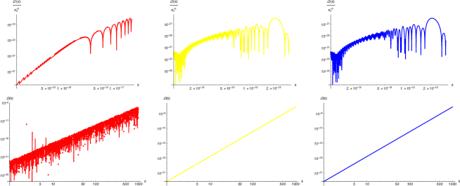
Figure 1: Three spectrum diagrams of $\Omega(k)$ corresponding to three cases of the Hubble parameter. $H^{2}(a)\approx H_{0}^{2}\Omega_{m}a^{-3}$ (red graph), $H^{2}(a)\approx H_{0}^{2}\left(\Omega_{m}a^{-3}+\Omega_{\Lambda}\right)$ (yellow graph) and $H^{2}(a)=H_{0}^{2}\left(\Omega_{r}a^{-4}+\Omega_{m}a^{-3}+\Omega_{\Lambda}\right)$ (blue graph). The difference between the figures in the top and bottom rows is only in the presented frequency ranges.

1) General case: $H^{2}(a)=H_{0}^{2}\left(\Omega_{r}a^{-4}+\Omega_{m}a^{-3}+\Omega_{\Lambda}\right)$ corresponds to the blue graph,
2) Matter–Dark Energy dominate case: $H^{2}(a)\approx H_{0}^{2}\left(\Omega_{m}a^{-3}+\Omega_{\Lambda}\right)$ corresponds to the yellow graph,
3) Matter dominate case: $H^{2}(a)\approx H_{0}^{2}\Omega_{m}a^{-3}$ corresponds to the red graph.
The two simple can be deduced by looking at the figure:
1) All cases are compatible with the Big Bang Nucleosynthesis (BBN) bounds which states that in frequency band around 100 Hz or $k=\frac{2\pi f}{c}\simeq 628\hskip 1.42262ptm^{-1}$ (in $c=1$ unity), $\Omega_{gw}(f)\leq 6.9\times 10^{-6}$ [12]. For a better benchmark, the values of $\Omega$ for this frequncy are given in the Table.1.
2) The graphs corresponding to the cases (1), (2) (yellow and blue graphs) are not much different and this is to be expected due to the insignificant contribution of radiation term ($\Omega_{r}\simeq 10^{-4}$) in comparison with matter and dark energy contributions.

3.1 Dark Energy Effects

In this subsection, we discuss impact of dark energy contribution on spectrum diagrams. In order to this, the diagrams corresponding to matter–dominate (red diagram) and matter–dark energy dominate (yellow diagram) cases are redrawn in Fig.2. The difference with Fig.1 is only in the presented range frequency. The figure says about two effects of dark energy contribution with respect to the matter dominate case:
1) It increases SED in the initial frequencies and decreases it in high frequencies.
2) It increases the number of power fluctuations in the initial frequencies and at high frequencies, this situation is reversed. (spectrum fluctuations means the number of fluctuations in a frequency interval.)
In the end of the section, we note from an astrophysical and phenomenological point of view, the allowed constraints on $\Omega(k)$ (as BBN or observations of millisecond pulsars) can restrict the values for Cosmological Constant or other (inflationary) parameters as expansion rate in the inflationary epoch. This depends on the future detections of primordial GW by the new generations of the advanced technological instruments.

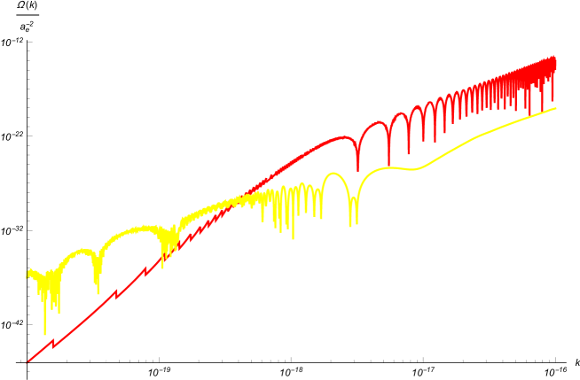
Figure 2: Dark energy contribution effects, $H^{2}(a)\approx H_{0}^{2}\Omega_{m}a^{-3}$ (red graph) and $H^{2}(a)\approx H_{0}^{2}\left(\Omega_{m}a^{-3}+\Omega_{\Lambda}\right)$ (yellow graph) .

Table 1: Numerical values of SED at $k\simeq 628$

$\frac{H^{2}(a)}{H_{0}^{2}}$	$\Omega(k\simeq 628)$
$\Omega_{m}a^{-3}$	$5.83\times 10^{-10}$
$\Omega_{m}a^{-3}+\Omega_{\Lambda}$	$2.29\times 10^{-9}$
$\Omega_{r}a^{-4}+\Omega_{m}a^{-3}+\Omega_{\Lambda}$	$2.28\times 10^{-9}$

4 Conclusions

In the very early universe, tensorial perturbations was amplified during the inflationary epoch leading to primordial radiation. The remnants of this radiation must exist in the present age as well and thus its detection can tell us the facts about the past history of the universe. An efficient quantity associated with the gravity waves detection is the radiation spectrum (or what is called in breif SED). In this work, SED of primordial gravity waves is calculated and presented by their corresponding diagrams in three cases of the Hubble expansion rate. The observations (data coming from the phenomenological and experimental bounds on the spectral energy) predict mostly growing character for the spectrum and this character is confirmed by the illustrated diagrams here. The graphs of spectrum are consistent with the observational data (as BBN bounds) and also indicate the dark energy has a decreasing (in high frequency) and an increasing (in low frequency) effect on the power spectrum.
Acknowledgments: We thank K. Rezazadeh for useful discussions.

References

- [1] A. Einstein, Sitzungsber. K. Preuss. Akad. Wiss. 1, 688 (1916).
- [2] L. Blanche, Living Rev. Relativity 17, (2014).
- [3] R. Jinno, T. Moroi and K. Nakayama, JCAP 1, 41(2014).
- [4] B. P. Abbott, et al, Phys. Rev. Lett 116, 061102(2016).
- [5] B. P. Abbott, et al, Phys. Rev. Lett 119, 141101(2017).
- [6] B. P. Abbott, et al, Phys. Rev. Lett 119, 161101(2017).
- [7] L. A. Boyle and P. J. Steinhardt, Phys. Rev. D 77, 063504 (2008).
- [8] Y. Watanabe and E. Komatsu, Phys. Rev. D 73, 123515(2006).
- [9] S. Weinberg, Phys. Rev. D 69, 023503(2004).
- [10] D. N. Spergel et al, ApJ Suppl 148, 175(2003).
- [11] S. Dodelson and F. Schmidt, Modern Cosmology, ACADEMIC PRESS, p-162, (2021).
- [12] B. P. Abbott et al. (LIGO Scientific Collaboration and Virgo Collaboration), Nature (London) 460, 990(2009).