Classifying topological sector via machine learning

Abstract:

We employ a machine learning technique for an estimate of the topological charge $Q$ of gauge configurations in SU(3) Yang-Mills theory in vacuum [1]. As a first trial, we feed the four-dimensional topological charge density with and without smoothing into the convolutional neural network and train it to estimate the value of $Q$. We find that the trained neural network can estimate the value of $Q$ from the topological charge density at small flow time with high accuracy. Next, we perform the dimensional reduction of the input data as a preprocessing and analyze lower dimensional data by the neural network. We find that the accuracy of the neural network does not have statistically-significant dependence on the dimension of the input data. From this result we argue that the neural network does not find characteristic features responsible for the determination of $Q$ in the higher dimensional space.

1 Introduction

The existence of nontrivial topology is one of the most important non-perturbative aspects of Quantum chromodynamics (QCD) and other Yang-Mills (YM) gauge theories in four spacetime dimensions. These theories can have topologically nontrivial gauge configurations classified by the topological charge $Q$. The topology in QCD is responsible for various non-perturbative properties of this theory, such as the U(1) problem [2].

The topological property of YM theories has been studied by numerical simulations of lattice gauge theory. Although gauge configurations on the lattice are strictly speaking topologically trivial, it is known that well separated topological sectors emerge as the continuum limit is approached [3]. It is known that the values of $Q$ of lattice gauge configurations measured by various methods show an approximate agreement [4], which is consistent with the existence of the well separated topological sectors in lattice gauge theory.

In the present study, we apply the machine learning (ML) for the analysis of $Q$ of gauge configurations on the lattice [1]. We generate data by the numerical simulation of SU(3) YM theory in four spacetime dimensions, and feed them into the neural networks (NN). The main motivation of this study is the search for characteristic local structures in the four-dimensional space related to $Q$ by the ML. It is known that YM theories have classical gauge configurations called instantons, which carry a nonzero topological charge and have a localized structure [2]. If the topological charge of the quantum gauge configurations is also carried by instanton-like local objects, the NN would recognize and make use of them for the prediction of $Q$. This study will also contribute to a reduction of the numerical costs for the analysis of $Q$.

2 Topological charge and gradient flow

In this study, we consider SU(3) YM theory in the four-dimensional Euclidean space with the periodic boundary conditions for all directions. The Wilson gauge action is used for generating gauge configurations. The numerical analyses are performed at two inverse couplings $\beta=6/g^{2}=6.2$ and $6.5$ with the lattice volumes $16^{4}$ and $24^{4}$, respectively, and $20,000$ gauge configurations have been generated for each analysis. These two lattices have almost the same physical volume.

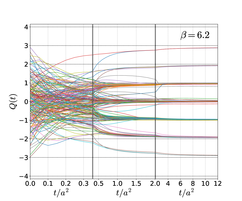
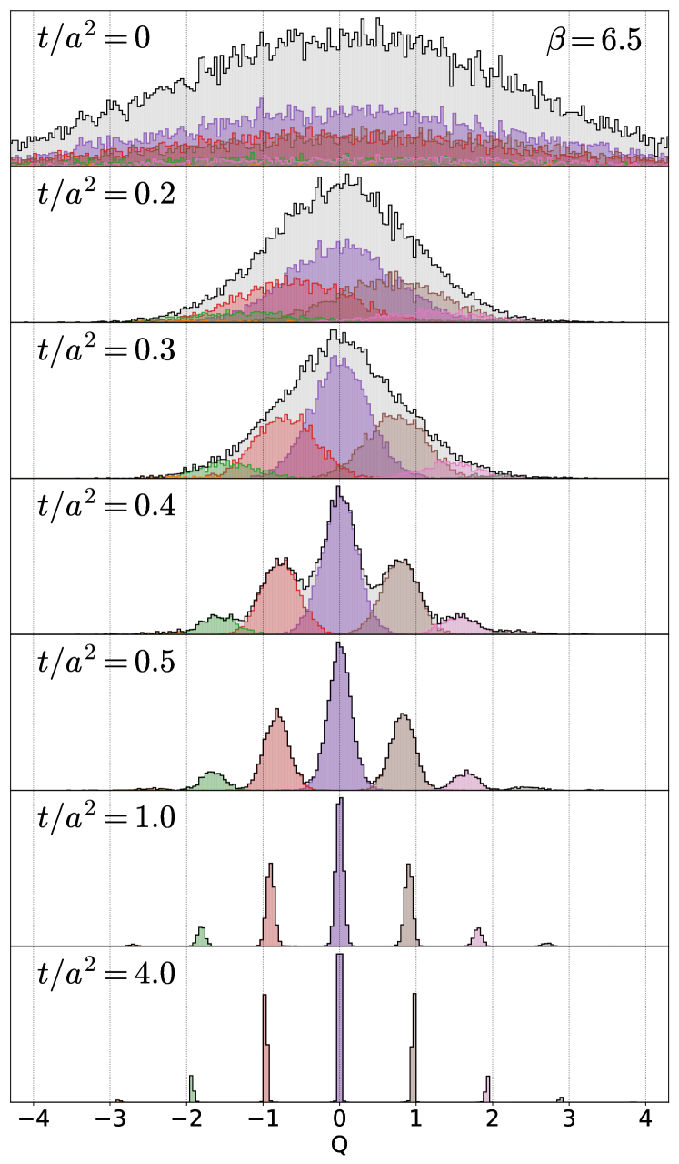
Figure 1: Left: Flow time $t$ dependence of $Q(t)$ on $200$ gauge configurations at $\beta=6.2$ (upper) and $6.5$ (lower). Right: Distribution of $Q(t)$ at several values of $t/a^{2}$. The colored histograms are the distributions in individual topological sectors.

In the continuous YM theory the topological charge is defined by

$$Q=\int_{V}d^{4}x\,q(x),\qquad q(x)=-\frac{1}{32\pi^{2}}\epsilon_{\mu\nu\rho\sigma}{\rm tr}\left[F_{\mu\nu}(x)F_{\rho\sigma}(x)\right],$$ (1)

with the field strength $F_{\mu\nu}(x)=\partial_{\mu}A_{\nu}(x)-\partial_{\nu}A_{\mu}(x)+[A_{\mu}(x),A_{\nu}(x)]$ and $q(x)$ the topological-charge density. In lattice gauge theory, Eq. (1) calculated on a gauge configuration is not given by an integer, but distributes continuously. To obtain discretized values, one may apply a smoothing of the gauge field before the measurement of $q(x)$. In the present study, we use the gradient flow [5] for the smoothing. The gradient flow is a transformation of the gauge field described by a continuous parameter $t$ called the flow time. The gauge field at a flow time $t$ is a smoothed field with the mean-square smoothing radius $\sqrt{8t}$ [5]. We denote the topological charge density at $t$ as $q_{t}(x)$, and its four-dimensional integral as

$$Q(t)=\int_{V}d^{4}x\,q_{t}(x).$$ (2)

In the left panels of Fig. 1, we show $200$ examples of $Q(t)$ for $\beta=6.2$ and $6.5$. The horizontal axis shows $t/a^{2}$ with the lattice spacing $a$. The panels show that $Q(t)$ approaches discrete integer values as $t$ becomes larger. In the right panel of Fig. 1, we show the distribution of $Q(t)$ at $\beta=6.5$ for several values of $t/a^{2}$ by the histogram. Although the values of $Q(t)$ are distributed continuously around the origin at $t=0$, the distribution converges on discretized integer values as $t$ becomes larger. At $t/a^{2}\gtrsim 1.0$, the gauge configurations are well separated into different topological sectors. We define the topological charge from $Q(t)$ at $t/a^{2}=4.0$ as

$$Q={\rm round}[Q(t)]_{t/a^{2}=4.0},$$ (3)

where ${\rm round}(x)$ means rounding off to the nearest integer. As indicated from Fig. 1, the value of $Q$ in Eq. (3) hardly changes with the variation of $t/a^{2}$ in the range $t/a^{2}\gtrsim 4$. It is known that the topological charge $Q$ defined in this way approximately agrees with those obtained through other definitions [4]. In the right panel of Fig. 1, the distributions of $Q(t)$ in individual topological sectors are shown by the colored histograms. From the panel one sees that the distribution of $Q(t)$ deviates from integer values toward the origin. This deviation becomes smaller as $t$ becomes larger.

3 Benchmark

In this study, we evaluate the performance of a model for an estimate of $Q$ by the accuracy $P$ and recalls $R_{Q}$ defined by

$$P=\frac{N_{\rm correct}}{N_{\rm total}},\qquad R_{Q}=\frac{N_{Q}^{\rm correct}}{N_{Q}},$$ (4)

where $N_{\rm total}$, $N_{\rm correct}$, $N_{Q}$, and $N_{Q}^{\rm correct}$ mean the numbers of total data, total correct answers, data in the topological sector $Q$, and correct answers among them, respectively. The recalls are suitable to see the bias of the answers.

$t/a^{2}$	$\beta=6.2$	$\beta=6.5$
0	0.273(3)	0.162(3)
0.1	0.383(4)	0.274(3)
0.2	0.546(4)	0.474(4)
0.3	0.773(3)	0.713(4)
0.4	0.925(2)	0.916(2)

$t/a^{2}$	$\beta=6.2$	$\beta=6.5$
0.5	0.960(1)	0.989(1)
1.0	0.982(1)	0.999(0)
2.0	0.992(1)	0.999(0)
4.0	1.000(0)	1.000(0)
10.0	0.993(1)	0.999(0)

Table 1: Accuracy $P_{\rm imp}$ obtained by the model Eq. (6) with the optimized parameter $c$.

In this study, we analyze $q_{t}(x)$ or $Q(t)$ at small $t$ by the NN. Here, $t$ used for the input has to be chosen small enough so that a simple estimate of $Q$ like Eq. (3)

$$Q_{\rm naive}={\rm round}[Q(t)],$$ (5)

does not give a high accuracy. We also consider an improved estimator of $Q$ defined by

$$Q_{\rm imp}={\rm round}[cQ(t)],$$ (6)

where $c$ is a parameter determined so as to maximize the accuracy in the range $c>1$ for each $t$. This parameter is introduced to compensate the deviation of the distribution of $Q(t)$ in each topological sector from integers found in Fig. 1. We found that Eq. (6) with the optimized $c$ has a better accuracy compared with the naive model Eq. (5) at some range of $t/a^{2}$. In Table 1, we show the accuracy $P_{\rm imp}$ of the model Eq. (6) for several values of $t/a^{2}$. We note that $P_{\rm naive}=P_{\rm imp}=1$ at $t/a^{2}=4.0$ by definition. As the accuracy is almost unity at $t/a^{2}=2.0$ and $10.0$, the value of $Q$ defined by Eq. (3) hardly changes with the variation of $t/a^{2}$ in the range $t/a^{2}\gtrsim 2.0$.

4 Analysis of four-dimensional field

layer	filter size	output size
input	-	$8^{d}\times N_{\rm ch}$
convolution	$3^{d}$	$8^{d}\times 5$
convolution	$3^{d}$	$8^{d}\times 5$
convolution	$3^{d}$	$8^{d}\times 5$
global average pooling	$8^{d}$	$1\times 5$
full connect	-	5
full connect	-	1

layer	output size
input	3
full connect	5
full connect	1

Table 2: Designs of the NN. In Secs. 4 and 6 we use the convolutional NN in the left panel with the dimension $d$ of the input data, while in Sec. 5 a simple fully-connected NN in the right panel is employed.

In this section, we analyze the four-dimensional data of $q_{t}(x)$ by the ML. We feed the topological charge density $q_{t}(x)$ into the NN and train it by the supervised learning so that it answers the value of $Q$ defined by Eq. (3). We employ the convolutional NN (CNN) for four-dimensional space. As the CNN is a class of NNs which had been developed for the image recognition [6, 7], this framework would be suitable for searching for local features in the four-dimensional data.

The structure of the CNN is shown in the left panel of Table 2. The lattice volume is reduced to $8^{4}$ from $16^{4}$ and $24^{4}$ by the average pooling by a preprocessing. The CNN has three convolutional layers with the filter size $3^{4}$ and five output channels. The global average pooling (GAP) layer, which takes the average with respect to the spatial coordinates, is inserted after the convolutional layers to respects the translational symmetry of the input data. The output of the GAP layer is then processed by two fully-connected layers. For more details on the NN and the procedure of the supervised learning, see Ref. [1].

In the upper four rows of Table 3, we show the resulting accuracy $P$ and recall of each topological sector $R_{Q}$ with the input data at several flow times $t$ for $\beta=6.5$. At $t=0$, the accuracy takes a nonzero value $P\simeq 0.39$. However, from the values of $R_{Q}$ one finds that the NN answers $Q=0$ for almost all gauge configurations. This result shows that the CNN does not find any useful features in the input data.

			$R_{Q}$
$N_{\rm ch}$	input $t/a^{2}$	$P$	-4	-3	-2	-1	0	1	2	3	4
1	0	0.388	0	0	0	0	1.000	0	0	0	0
1	0.1	0.396	0	0	0	0.086	0.889	0.129	0	0	0
1	0.2	0.479	0	0	0.108	0.445	0.641	0.459	0.150	0	0
1	0.3	0.698	0	0.170	0.585	0.730	0.727	0.701	0.624	0.395	0.071
3	0.3,0.2,0.1	0.953	0	0.830	0.951	0.956	0.952	0.962	0.968	0.953	0.286

Table 3: Accuracy $P$ and the recalls of individual topological sectors $R_{Q}$ obtained by the analysis of $q_{t}(x)$ in the four-dimensional space by the CNN for $\beta=6.5$. The input data has $N_{\rm ch}$ channels.

Because the analysis of the data at $t=0$ does not provide any useful results, as a next trial we perform the analysis of $q_{t}(x)$ at nonzero $t$. The resulting accuracy and recalls at $t/a^{2}=0.1$, $0.2$, and $0.3$ depicted in Table 3 shows that the accuracy becomes better as $t/a^{2}$ becomes larger. From the behavior of $R_{Q}$ one also finds that the answers of the CNN are distributed for all topological sectors at large $t/a^{2}$. From this result, it is naïvely expected that the CNN recognizes features in the four-dimensional space. However, by comparing these accuracies with Table 1, one finds that the accuracies are almost consistent with the benchmark model Eq. (6) at the same $t/a^{2}$. A natural interpretation of this result is that the answers of the CNN are obtained by Eq. (6). Because the four-dimensional structure is completely integrated out in Eq. (6), this result shows that characteristic features responsible for the determination of $Q$ in the four-dimensional space were not found by the CNN.

In order to realize the recognition of the four-dimensional data by the CNN, we next feed $q_{t}(x)$ obtained at three different flow times simultaneously as a single multi-channel data. We use $q_{t}(x)$ at $t/a^{2}=0.3$, $0.2$, and $0.1$ for the input. The resulting accuracy and recalls are shown at the bottom row of Table 3. One finds a remarkable improvement of the accuracy compared with the analysis of the single flow time, which indicates a nontrivial recognition of the four-dimensional data by the CNN.

5 Analysis of $Q(t)$

Let us inspect whether the high accuracy of the CNN in the previous section is established by the recognition of the four-dimensional space, or not. For this purpose, in this section we consider a simple fully connected NN (FNN) which accepts only three values of $Q(t)$ at different $t/a^{2}$. The structure of the FNN is shown in the right panel of Table 2. The FNN has only one hidden layer that is fully connected with the input and output layers.

input $t/a^{2}$	$\beta=6.2$	$\beta=6.5$
0.35, 0.3, 0.25	0.967(2)	0.996(1)
0.3, 0.25, 0.2	0.959(2)	0.990(2)
0.25, 0.2, 0.15	0.939(3)	0.951(2)
0.3, 0.2, 0.1	0.941(2)	0.957(2)

Table 4: Accuracy of the trained FNN in Table 2 with various sets of the input data. Left column shows the values of $t/a^{2}$ that evaluate $Q(t)$ for the input. Errors are estimated from the variance among 10 different trainings.

In Table 4, we show the accuracies obtained by the trained FNN for various combinations of the flow times for the input $Q(t)$ at $\beta=6.2$ and $6.5$. The table shows that the accuracy with the combination $t/a^{2}=(0.3,0.2,0.1)$ is comparable with that obtained in the previous section, although the four-dimensional structure of the input data is fully integrated out in this analysis. From this result it is concluded that the CNN in Sec. 4 does not find features in the four-dimensional space, but performs almost the same analysis as the FNN introduced in this section.

Table 4 also suggests that the accuracy obtained by the FNN is significantly higher than $P_{\rm imp}$ with the same largest $t/a^{2}$. In particular, the accuracy with $t/a^{2}=(0.3,0.25,0.2)$ shown by the bold letters is as high as $99\%$ for $\beta=6.5$, while the benchmark model Eq. (6) gives $P_{\rm imp}\simeq 0.71$ at $t/a^{2}=0.3$. This result shows that the trained NN can estimate $Q$ quite successfully only with the data at $t/a^{2}\lesssim 0.3$, and this model can be used for an effective analysis of $Q$. The robustness of this result against the variation of the lattice spacing and the effect of the reduction of the training data are discussed in Ref. [1].

6 Dimensional reduction

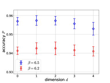
Figure 2: Dependence of the accuracy $P$ on the dimension $d$ of the input data.

In Secs. 4 and 5, we analyzed the data with the space dimension $d=4$ and $0$, respectively. We next consider the analysis of the data with dimensions $d=1$–$3$ by the NN. We reduce the dimension of the input data by the dimensional reduction, i.e. by integrating out some coordinates, and explore a possible optimal dimension of the input data of the CNN between $d=0$ and $4$.

In Fig. 2, we show the dependence of the resulting accuracy of the trained CNN on $d$ with the flow times of the input data $t/a^{2}=(0.3,0.2,0.1)$. The figure shows that the accuracy does not have a statistically-significant $d$ dependence, although the results at $d=1$ and $2$ would be slightly better. This result supports our observation that the CNN does not recognize features in the multi dimensional space.

7 Summary

In this study, we applied a machine learning technique for the classification of the topological sector of gauge configurations in SU(3) YM theory. We found that the value of $Q$ defined at a large flow time can be predicted with high accuracy only with $Q(t)$ at $t/a^{2}\leq 0.3$ with the aid of the NN. This procedure would be used for reducing the numerical cost for the analysis of $Q$. We also found that the analysis of the multi dimensional field $q_{t}(x)$ by the CNN does not improve the accuracy, which suggests that our CNN fails in capturing useful structures in the multi dimensional space.

The lattice simulations of this study are in part carried out on OCTOPUS at the Cybermedia Center, Osaka University. The NNs are implemented by Chainer framework, and are in part trained on Google Colaboratory. This work was supported by JSPS KAKENHI Grant Numbers 17K05442 and 19H05598.

References

- [1] T. Matsumoto, M. Kitazawa and Y. Kohno, Classifying Topological Charge in SU(3) Yang-Mills Theory with Machine Learning, 1909.06238.
- [2] S. Weinberg, The quantum theory of fields. Vol. 2: Modern applications. Cambridge University Press, 2013.
- [3] M. Luscher, Topology of Lattice Gauge Fields, Commun. Math. Phys. 85 (1982) 39.
- [4] C. Alexandrou, A. Athenodorou, K. Cichy, A. Dromard, E. Garcia-Ramos, K. Jansen et al., Comparison of topological charge definitions in Lattice QCD, arXiv:1708.00696 (2017) [1708.00696].
- [5] M. Luscher and P. Weisz, Perturbative analysis of the gradient flow in non-abelian gauge theories, JHEP 02 (2011) 051 [1101.0963].
- [6] Y. Lecun, L. Bottou, Y. Bengio and P. Haffner, Gradient-based learning applied to document recognition, Proc. IEEE 86 (1998) 2278.
- [7] A. Krizhevsky, I. Sutskever and G. E. Hinton, Imagenet classification with deep convolutional neural networks, NIPS’12, (USA), pp. 1097–1105, Curran Associates Inc., 2012.