Microscopic theory of pseudogap phenomena and unconventional Bose-liquid superconductivity and superfluidity in high-$T_{c}$ cuprates and other systems

Abstract

In this work, the consistent, predictive and empirically adequate microscopic theory of pseudogap phenomena and unconventional Bose-liquid superconductivity (superfluidity) is presented, based on the fact that in high-$T_{c}$ cuprates and other related systems the energy $\varepsilon_{A}$ of the effective attraction between fermionic quasiparticles is comparable with their Fermi energy $\varepsilon_{F}$ and the bosonic Cooper pairs are formed above $T_{c}$ (the temperature of the superfluid transition) and then a small part of such Cooper pairs condense into a Bose superfluid at $T_{c}$. According to this theory, the doped high-$T_{c}$ cuprates and other systems with low Fermi energies ($\varepsilon_{F}\sim\varepsilon_{A}$) are unconventional bosonic superconductors/superfluids and exhibit pseudogap phases above $T_{c}$, $\lambda$-like superconducting transition at $T_{c}$ and Bose-liquid superconductivity below $T_{c}$. The relevant charge carriers in high-$T_{c}$ cuprates are polarons which are bound into bosonic Cooper pairs above $T_{c}$. Polaronic effects and related pseudogap weaken with increasing the doping and disappear at a quantum critical point where a small Fermi surface of polarons transforms into a large Fermi surface of quasi-free carriers. The modified BCS-like theory describes another pseudogap regime but the superconducting/superfluid transition in high-$T_{c}$ cuprates and related systems is neither the BCS-like transition nor the usual Bose-Einstein condensation. A good quantitative agreement is found between pseudogap theory and experiment. Universal criteria for bosonization of Cooper pairs are formulated in terms of two fundamental ratios $\varepsilon_{A}/\varepsilon_{F}$ and $\Delta_{F}/\varepsilon_{F}$ (where $\Delta_{F}$ is the BCS-like gap). The mean-field theory of the coherent single particle and pair condensates of bosonic Cooper pairs describes fairly well the novel superconducting states (i.e., two distinct superconducting A and B phases below $T_{c}$ and a vortex-like state above $T_{c}$) and various salient features ($\lambda$-like transition at $T_{c}$, kink-like anomalies in all superconducting/superfluid parameters near the first-order phase transition temperature $T^{*}_{c}$ lower than $T_{c}$, gapless excitations below $T^{*}_{c}$ and two-peak specific heat anomalies) of high-$T_{c}$ cuprates in full agreement with the experimental findings. Though Bose-liquid superconductivity in the bulk of high-$T_{c}$ cuprates is destroyed at $T_{c}$, but it can persist above $T_{c}$ at grain boundaries and interfaces of these materials up to room temperature. The unusual superconducting/superfluid states and properties of other exotic systems (e.g., heavy-fermion and organic compounds, $\rm{Sr_{2}RuO_{4}}$, ³He, ⁴He and atomic Fermi gases) are explained more clearly by the theory of Bose superfluids. Finally, the new criteria and principles of unconventional superconductivity and superfluidity are formulated.

I I. INTRODUCTION

The usual band theory has been successful enough in describing the normal state of conventional metals with large Fermi energies $\varepsilon_{F}>1$ eV 1 ; 2 , while the theory of superconductivity proposed by Bardeen-Cooper-Schrieffer (BCS) 3 was quite adequate for the description of the Fermi-liquid superconductivity in these systems. However, the unconventional superconductivity (superfluidity) and the pseudogap phenomena discovered in doped high-$T_{c}$ copper oxides (cuprates) 4 ; 5 ; 6 ; 7 ; 8 ; 9 and other systems (e.g., liquid ³He, heavy-fermion and organic compounds, $\rm{Sr_{2}RuO_{4}}$ and ultracold atomic Fermi gases) 10 ; 11 ; 12 ; 13 ; 14 ; 15 ; 16 ; 17 ; 18 were turned out the most intriguing puzzles in condensed matter physics. The normal state of high-$T_{c}$ cuprates exhibits many unusual properties not encountered before in conventional superconductors, which are assumed to be closely related to the existence of a pseudogap predicted first theoretically 19 ; 20 ; 21 ; 22 ; 23 , and then, observed clearly experimentally 6 ; 7 ; 8 ; 9 . The normal state of other exotic superconductors 16 ; 18 ; 24 ; 25 and superfluids 26 also exhibits a pseudogap behavior above the superconducting/superfluid transition temperature $T_{c}$. The pseudogap phenomenon observed in high-$T_{c}$ cuprates and other systems means the suppression of the density of states at the Fermi level and the pseudogap appears at a characteristic temperature $T^{*}$ above $T_{c}$ without the emergence of any superconducting order. Most importantly, the high-$T_{c}$ cuprates in the intermediate doping regime exhibit exotic superconducting properties inherent in unconventional superconductors 17 ; 27 ; 28 ; 29 and quantum liquids (³He and ⁴He) 30 ; 31 ; 32 ; 33 , while the heavily overdoped cuprates are similar to conventional metals 34 ; 35 .

In the case of high-$T_{c}$ cuprates which are prototypical unconventional superconductors/superfluids and are of significant current interest in condensed matter physics and beyond (e.g., in the physics of low-density nuclear matter 36 ), our understanding of superconductivity and pseudogap phenomena is still far from satisfactory. Aside from early theoretical ideas 19 ; 20 ; 21 ; 22 ; 23 ; 37 ; 38 ; 39 ; 40 ; 41 , later other competing theories have been proposed for explaining the origins and the nature of the pseudogaps and high-$T_{c}$ superconductivity in these most puzzling materials (for a review see Refs. 35 ; 42 ; 43 ; 44 ; 45 ; 46 ; 47 ; 48 ). But in judging the relevance of these theoretical approaches to the unconventional cuprate superconductors with small Fermi energies $\varepsilon_{F}<<1$ eV, one should consider their compatibility with the observed normal-state properties, and especially superconducting properties (i.e., a $\lambda$-like superconducting transition at $T_{c}$, a first-order phase transition in the superconducting state and the kink-like temperature dependences of all superconducting parameters) of high-$T_{c}$ cuprates.

In high-$T_{c}$ cuprates and other complex systems, unconventional interactions between pairs of quasiparticles may take place, leading to new and unidentified states of matter. Specifically, the enigmatic pseudogap, diamagnetic and vortex-like states are formed in high-$T_{c}$ cuprate superconductors above $T_{c}$ 35 ; 45 ; 47 ; 49 , while the unusual superconducting state (see Fig. 1 in Refs.21 ; 51 ) and quantum critical point (QCP) (at $T=0$) exist below $T_{c}$ 52 ; 53 ; 54 ; 55 . The origin of the pseudogap state in these systems has been debated for many years, being attributed to the different pairing effects in the electronic subsystem 19 ; 21 ; 22 ; 23 ; 44 ; 46 and spin subsystem 37 ; 39 ; 56 or to other effects associated with different competing orders (see Refs. 35 ; 46 ). The pseudogap phenomena and high-$T_{c}$ cuprate superconductivity are often discussed in terms of superconducting fluctuation theories 19 ; 23 ; 46 ; 57 . The first proposed theory argues 19 that the superconducting fluctuation scenario is justifiable only for temperatures well below the onset temperature of Cooper pairing $T^{*}$ in the normal state of high-$T_{c}$ cuprates. Other superconducting fluctuation theories are believed to be less justifiable (see, e.g., Refs. 35 ; 42 ), since they assume that the superconductivity is destroyed at $T_{c}$ by the phase fluctuation, whereas local superconducting Cooper pairs persist well above $T_{c}$ 46 ; 49 or even up to the characteristic temperature $T^{*}>>T_{c}$ 23 ; 57 . In these theoretical scenarios, it is speculated that the BCS-like ($s$-or $d$-wave) gap represents the superconducting order parameter below $T_{c}$ and then persists as a superconductivity-related pseudogap above $T_{c}$, i.e., the superconducting BCS transition has a wide fluctuation region above $T_{c}$. However, the experimental data show that the pseudogap in high-$T_{c}$ cuprates is unrelated to superconducting fluctuations 58 and the superconducting transition is a $\lambda$-transition 33 ; 59 ; 60 and it is characterized by a narrow fluctuation region ($T-T_{c}\lesssim 0.1T_{c}$) above $T_{c}$ 35 ; 42 . Another inconsistency is that the problem of quantitative determination of $T_{c}$ in these unconventional superconductors remains unresolved and the phenomenological Ginzburg-Landau or Kosterlitz-Thouless theory is used to determine the actual $T_{c}$ 19 ; 23 ; 49 . In reality, the pseudogap state in high-$T_{c}$ cuprates has properties incompatible with superconducting fluctuations 35 ; 42 ; 58 and most likely behaves as an anomalous metal above $T_{c}$ 21 ; 35 ; 62 ; 63 .

In alternative theoretical scenarios, the unconventional (i.e. non-superconducting) Cooper pairing can be expected in the low carrier concentration limit at $T=2T_{c}$ in superconducting semiconductors 64 and in underdoped cuprates in a wide temperature range above $T_{c}$ 21 ; 22 ; 62 . Such a Cooper pairing of fermionic quasiparticles (e.g., polarons) in the normal state of high-$T_{c}$ cuprates can occur in the BCS regime and lead to the formation of a non-superconductivity-related pseudogap. In this case, one expects the preformed Cooper pairs exist in the bosonic limit.

Attempts to understand the different pseudogap regimes in high-$T_{c}$ cuprates have been based on the different temperature-doping phase diagrams showing only one pseudogap crossover temperature 37 ; 47 ; 52 ; 65 or two pseudogap crossover temperatures 56 ; 62 ; 63 ; 66 ; 67 above $T_{c}$ and a QCP under the superconducting dome at $T=0$ 52 ; 62 ; 65 ; 67 . However, a full description of the distinctive phase diagrams and the pseudogap, quantum critical and unusual superconducting states of these intricate materials in the different competing theories is still out of reach (see, e.g., question marks in the proposed phase diagrams of the cuprates 37 ; 45 ; 68 ). Because many of the proposed theories are phenomenological in nature and fail to explain consistently not only the existence of different pseudogap regimes above $T_{c}$, pseudogap QCPs under the superconducting dome and distinct superconducting regimes below $T_{c}$, but also all the anomalies observed in the normal and superconducting properties of various high-$T_{c}$ cuprates.

Many theoretical scenarios for high-$T_{c}$ cuprate superconductivity are based on the BCS-like pairing correlations and on the usual Bose-Einstein condensation (BEC) of an ideal Bose-gas of Cooper pairs and other bosonic quasiparticles (e.g., bipolarons and holons). However, the BCS-type ($s$-, $p$- or $d$- wave) superconductivity is most likely to occur in systems that satisfy at least the following three conditions. First, they should have large Fermi energies. Second, the attractive interaction between pairs of fermionic quasiparticles near Fermi surface must be sufficiently weak. Third, the Cooper pairs should have fermionic nature due to their strong overlapping just like in metals. The transition from BCS-type condensation regime to BEC regime can be expected in a Fermi system, if either the attractive interaction between fermions is increased sufficiently or the density of fermions is decreased to a certain critical density. Such a transition was studied, first, in superconducting semiconductors (where the Cooper pairing without superconductivity at low carrier concentrations may occur) 64 and then in an attractive Fermi gas 69 ; 70 . The high-$T_{c}$ cuprates and many other exotic systems may fail to meet the above three conditions needed for BCS-type superconductivity and superfluidity. Some theoretical models of high-$T_{c}$ cuprate superconductivity 44 ; 71 ; 72 based on the BCS-BEC crossover 64 ; 69 ; 70 interpolate between BCS-like transition in Fermi liquid and usual BEC of preformed Cooper pairs as the interaction strength is varied. However, according to the Landau criterion 30 , the usual BEC of an ideal Bose gas of small real-space pairs and Cooper pairs is irrelevant to the superconductivity (superfluidity) phenomenon. Also, it was clearly argued by Evans and Imry 73 that the superfluid phase in ⁴He is not described by the presence of BEC in an ideal or a repulsive Bose gas of ⁴He atoms.

Successful solutions of complex problems posed by high-$T_{c}$ cuprate superconductors may provide new insights into the microscopic physics and thus contribute toward a complete understanding of unsolved problems of other unconventional superconductors and superfluids. So far, the pseudogap phenomena and unconventional superconductivity (superfluidity) in high-$T_{c}$ cuprates and other systems are often misinterpreted. In particular, the high-$T_{c}$ cuprates are similar to the superfluid ⁴He and might be genuine superfluid Bose systems that cannot be understood within the BCS-like and BEC theories. Further, the superconductivity in other exotic systems and the superfluidity both in ³He and in ultracold atomic Fermi gases with an extremely high superfluid transition temperature with respect to the Fermi temperature $T_{F}\simeq 5T_{c}$ 26 cast a doubt on any BCS-like pairing theory as a complete theory of these phenomena.

The purpose of this paper is to construct a consistent, predictive and empirically adequate microscopic theory of pseudogap phenomena and unconventional Bose-liquid superconductivity and superfluidity, which accounts for essentially all the observed pseudogap features and novel superconducting/superfluid properties of high-$T_{c}$ cuprates and other intricate systems. By studying the ground states of doped charge carriers in polar cuprate materials, we show that the relevant charge carriers in such systems are large polarons. Polaronic effects in doped high-$T_{c}$ cuprates can give rise to a pseudogap state and a polaronic pseudogap weakens with increasing the doping and disappear at a specific QCP. We demonstrate that the pairing theory of polarons in real-space describes the formation of large bipolarons at low dopings, while the modified BCS-like pairing theory describes the formation of bosonic Cooper pairs at intermedate dopings in these systems. Our results provide deeper insights into the emergence of the two different pseudogap regimes above $T_{c}$ and the pseudogap phase boundary terminating at specific QCPs in various high-$T_{c}$ cuprates and the pseudogap effects on the normal-state properties of high-$T_{c}$ cuprates. We then apply the BCS-like pairing theory to describe the pseudogap state in other unconventional superconductors and superfluids. For all cases considered, good quantitative agreement is found between pseudogap theory and experiment.

Next we address the key issue of whether Cooper pairs have fermionic nature just like in the BCS theory or they are bosonic quasiparticles. We formulate the universal criteria for bosonization of Cooper pairs in high-$T_{c}$ cuprates and other related systems using the uncertainty prinsiple. We then elaborate a consistent mean-field microscopic theory of Bose-liquid superconductivity and superfluidity by starting from the boson analogs of the BCS-like pair Hamiltonian. This theory describes the superfluidity in three-dimensional (3D) and two-dimensional (2D) attractive Bose systems originating from the pair condensation (at $T_{c}$) and single particle condensation (at a certain temperature $T^{*}_{c}$ below $T_{c}$ in 3D systems or at $T=0$ in 2D systems) of bosonic Cooper pairs and ⁴He atoms. The self-consistent solutions of mean-field integral equations for attractive 3D and 2D Bose systems are capable of giving the new predictions and the adequate description of the three distinct regimes of Bose-liquid superconductivity and superfluidity, $\lambda$-like superconducting transition at $T_{c}$, first-order phase transition at $T^{*}_{c}$, half-integer $h/4e$ magnetic flux quantization and two distinct superconducting phases below $T_{c}$, the novel gapless excitations below $T^{*}_{c}$ and vortex-like excitations above $T_{c}$ and other observed puzzling superconducting properties of high-$T_{c}$ cuprates. The unconventional superconductivity and superfluidity observed in other systems, such as in heavy-fermion and organic compounds, $\rm{Sr_{2}RuO_{4}}$, quantum liquids (³He and ⁴He) and atomic Fermi gases are also well described by the mean-field theory of Bose superfluids, while the mean-field theory of the BCS-like ($s$-, $p$-or $d$-wave) pairing of fermionic quasiparticle can describe only the formation of Cooper pairs in these intricate systems.

The rest of the paper is organized as follows. In Sec. II, the unconventional electron-phonon interactions, the new in-gap states and the relevant charge carriers in doped high-$T_{c}$ cuprate superconductors are described. In Sec. III, the microscopic theory of pseudogap phenomena in these high-$T_{c}$ materials is presented. In Sec. IV, the pseudogap effects on the normal-state properties of underdoped to overdoped cuprates are discussed. In Sec. V, the pseudogap phenomena in other systems are described. In Sec. VI, the problem of the bosonization of Cooper pairs in high-$T_{c}$ cuprates and other systems is solved. In Sec. VII, the mean-field theory of 3D and 2D superfluid Bose liquids is elaborated. In Sec. VIII, the microscopic theory of unconventional Bose-liquid superconductivity and superfluidity in high-$T_{c}$ cuprates and other systems is presented. In Sec. IX, the new criteria and principles of unconventional superconductivity and superfluidity are formulated. In Sec.X, we summarize our results. Computational details are presented in Appendixes.

II II. GROUND STATE ENERGIES OF CHARGE CARRIERS AND GAP-LIKE FEATURES IN DOPED CUPRATES

Since the discovery of high-$T_{c}$ superconductivity in doped cuprates 4 ; 5 , the nature and types of charge carriers, which determine the insulating, metallic and superconducting properties of these materials, have especially been the subject of controversy, being attributed to hypothetical quasiparticles 35 ; 74 ; 75 (e.g., holons and other electron- or hole-like quasiparticles) or self-trapped quasiparticles (large and small (bi)polarons) 44 ; 76 ; 77 ; 78 . The issues concerning the relevant charge carriers and the unusual unsulating, metallic and superconducting phases in some doped cuprates remain unresolved yet (see, e.g., question marks in some proposed phase diagrams of doped cuprates 37 ; 45 ; 68 ).

According to the Zaanen-Sawatzky-Allen classification scheme 79 , the electronic band structure of the undoped cuprates corresponds to the charge-transfer (CT)-type Mott-Hubbard insulators 80 ; 81 . Because the strong electron correlations (i.e., the strong Coulomb repulsions between two holes each on copper Cu sites) drive these systems into the Mott-Hubbard-type insulating state. As a result, the oxygen 2$p$ band in the undoped cuprates lies within the Mott-Hubbard gap and the Fermi level $\varepsilon_{F}$ is located at the center of the CT gap 81 . Hole carriers introduced by doping will not appear on copper sites giving two holes ($\rm{Cu^{3+}}$) (i.e. spinless holons 75 ) but they appear as quasi-free holes in the oxygen band instead, where the correlation between these holes is weak enough 74 . Actually, the preponderance of experimental evidence now supports the oxygen character of additional (i.e. doped) holes (see Refs. 80 ; 82 ). Upon hole doping, the oxygen valence band of the cuprates is occupied first by hole carriers having the effective mass $m^{*}$, which are delocalized just like in doped semiconductors (e.g., Si and Ge) and interact with acoustic and optical phonons. Therefore, the properties of the hole carriers in these polar materials are strongly modified by their interaction with the lattice vibrations (i.e. by strong and intermediate electron-phonon coupling) and they are self-trapped at their sufficiently strong coupling to optical phonons. Essentially, a large ionicity of the cuprates $\eta=\varepsilon_{\infty}/\varepsilon_{0}<<1$ (where $\varepsilon_{\infty}$ and $\varepsilon_{0}$ are the high-frequency and static dielectric constants, respectively) enhances the polar hole-lattice interaction and the tendency to polaron formation. One can expect that the the self-trapping of hole carriers in doped cuprates will be more favorable just like the self-trapping of holes in ionic crystals of alkali halides 83 ; 84 .

One distinguishes three distinct regimes of electron (hole)-phonon coupling in doped polar cuprates: (i) the weak-coupling regime in heavily overdoped cuprates describes the correlated motions of the lattice atoms and the quasi-free charge carriers which remain in their initial extended state, (ii) the intermediate-coupling regime (corresponding to the underdoped, optimally doped and moderately overdoped cuprates) characterizes the self-trapping of a charge carrier, which is bound within a potential well produced by the polarization of the lattice in the presence of the carrier and follows the atomic motions in the non-adiabatic regime, and (iii) the strong-coupling regime in lightly doped cuprates describes the other condition of self-trapping under which the lattice distortion cannot follow the charge carrier motion and the self-trapping of carriers is usually treated within the adiabatic approximation (i.e., the lattice atoms remain at their fixed positions). In the latter case the carrier is strongly bound to a lattice distortion by a strong and very localized carrier-lattice interaction. Under certain conditions, two charge carriers interacting with the lattice vibrations and with each other can form a bound state of two carriers in polar materials within a common self-trapping well. In these systems the attractive electron-phonon interaction can be strong enough to overcome the Coulomb repulsion between two charge carriers. The self-trapped state of the pair of charge carriers is termed as a bipolaron.

In the following, we will consider the self-trapping of hole carriers in the continuum model 85 ; 86 and adiabatic approximation taking into account both the short- and long-range carrier-phonon interactions in doped cuprates. In the case of the lightly doped cuprates, the total energies of the coupled hole-lattice and two-hole-lattice systems are given by the following functionals describing the formation of the polaronic and bipolaronic states 78 :

$$E_{p}{\{\psi\}}=\frac{\hbar^{2}}{2m^{*}}\int(\nabla\psi(r))^{2}d^{3}r-$$

$$-\frac{e^{2}}{2\tilde{\varepsilon}}\int\frac{\Psi^{2}(r)\Psi^{2}(r^{\prime})}{|\vec{r}-\vec{r}^{\prime}|}d^{3}rd^{3}r^{\prime}-\frac{E^{2}_{d}}{2B}\int\psi^{4}(r)d^{3}r,$$ (1)

and

$$E_{B}{\{\Psi}\}=\frac{\hbar^{2}}{2m^{*}}\int\big{[}(\nabla_{1}\Psi(r_{1},r_{2}))^{2}+$$

$$+(\nabla_{2}\Psi(r_{1},r_{2}))^{2}]d^{3}r_{1}d^{3}r_{2}+$$

$$+\frac{e^{2}}{\varepsilon_{\infty}}\int\frac{\Psi^{2}(r_{1},r_{2})}{|\vec{r_{1}}-\vec{r_{2}}|}d^{3}r_{1}d^{3}r_{2}-$$

$$-\frac{2e^{2}}{\tilde{\varepsilon}}\int\frac{\Psi^{2}((r_{1},r_{2})\Psi^{2}(r_{3},r_{4}))}{|\vec{r_{1}}-\vec{r_{3}}|}d^{3}r_{1}d^{3}r_{2}d^{3}r_{3}d^{3}r_{4}-$$

$$-\frac{2E^{2}_{d}}{B}\int\Psi(r_{1},r_{2})\Psi(r_{2},r_{3})d^{3}r_{1}d^{3}r_{2}d^{3}r_{3},$$ (2)

where $\psi(r)$ and $\Psi(r_{1},r_{2})$ are the one- and two-particle wave functions, respectively, $\vec{r}$ is the position vector of a carrier, $\tilde{\varepsilon}=\varepsilon_{\infty}/(1-\eta)$ is the effective dielectric constant, $E_{d}$ is the deformation potential of a carrier, $B$ is an elastic constant of the crystal lattice. Minimization of the functionals (II) and (II) with respect to $\psi(r)$ and $\Psi(r_{1},r_{2})$ would give the ground state energies of hole carriers in doped cuprates. We minimize these functionals by choosing the following trial functions:

$$\psi(r)=N_{1}\exp[(-\sigma r)],$$ (3)

$$\Psi(r_{1},r_{2})=N_{2}[1+\gamma(\sigma{|\vec{r_{1}}-\vec{r_{2}}|})]\exp[(-\sigma(r_{1}+r_{2})],$$ (4)

where $N_{1}=\sigma^{3/2}/\sqrt{\pi}$ and $N_{2}=\sigma^{3}/\pi\sqrt{C_{1}(\gamma)}$ are the normalization factors, $\sigma=\beta/a_{0}$, $C_{1}(\gamma)=1+\frac{35}{8}\gamma+6\gamma^{2}$ is the correlation coefficient, $\sigma$ and $\gamma$ are the variational parameters characterizing the carrier localization and the correlation between carriers, respectively, $a_{0}$ is the lattice constant.

Substituting Eqs. (3) and (4) into Eqs. (II) and (II), and performing the integrations in Eqs. (II) and (II), we obtain the following functionals:

$$E_{p}(\beta)=A[\beta^{2}-g_{s}\beta^{3}-g_{l}(1-\eta)\beta],$$ (5)

and

$$E_{B}(\beta,\gamma)=2A\frac{C_{2}(\gamma)}{C_{1}(\gamma)}\Bigg{\{}\beta^{2}-16g_{s}\frac{C_{3}(\gamma)}{C_{1}(\gamma)C_{2}(\gamma)}\beta^{3}-$$

$$-\frac{8}{5}g_{l}\left[2(1-\eta)\frac{C_{4}(\gamma)}{C_{1}(\gamma)C_{2}(\gamma)}-\frac{C_{5}(\gamma)}{C_{2}(\gamma)}\right]\beta\Bigg{\}},$$ (6)

where $A=\hbar^{2}/2m^{*}a^{2}_{0}$, $g_{s}=E^{2}_{d}/16\pi Ba^{3}_{0}A$ and $g_{l}=5e^{2}/16\varepsilon_{\infty}a_{0}A$ are the dimensionless short- and long-range carrier-phonon coupling constants, respectively,

$$C_{2}(\gamma)=1+\frac{25}{8}\gamma+4\gamma^{2},$$

$$C_{3}(\gamma)=\frac{1}{8}+\frac{185}{216}\gamma+\frac{4199}{1728}\gamma^{2}+\frac{8591}{2592}\gamma^{3}+\frac{477}{256}\gamma^{4},$$

$$C_{4}(\gamma)=\frac{5}{8}+\frac{1087}{216}\gamma+\frac{38237}{2304}\gamma^{2}+\frac{67639}{2592}\gamma^{3}+\frac{4293}{256}\gamma^{4},$$

$$C_{5}(\gamma)=\frac{5}{8}+2\gamma+\frac{35}{16}\gamma^{2}.$$

By minimizing the functionals (5) and (II) with respect to $\beta$ and $\gamma$, we determine the ground state energies of hole carriers and the polaronic and bipolaronic states lying in the CT gap of the cuprates.

II.1 A. Basic parameters of strong coupling large polarons and bipolarons

We now calculate the ground state energies of strong coupling large polarons and bipolarons in lightly doped cuprates using the values of the parameters entering into Eqs. (5) and (6). The lattice parameter value of the orthorhomic cuprates is about $a_{0}\simeq 5.4{\AA}$. According to the spectroscopy data, the Fermi energy $E_{F}$ of the undoped cuprates is equal to 7 eV 87 . To determine the value of the short-range carrier-phonon coupling constant $g_{s}$, we can estimate the deformation potential as $E_{d}=(2/3)E_{F}$ 88 . For the cuprates, typical values of other parameters are $m^{*}\simeq m_{e}$ 89 (where $m_{e}$ is the free electron mass), $\varepsilon_{\infty}=3-5$ 76 ; 90 , $\varepsilon_{0}\simeq 22-85$ 76 ; 77 ; 90 , $B\approx 1.4\cdot 10^{12}dyn/cm^{2}$ 91 . The minima of $E_{p}(\beta)$ and $E_{B}(\beta,\gamma)$ correspond to the ground state energies of strong coupling large polaron and bipolaron, respectively, which are measured with respect to the top of the oxygen valence band. The basic parameter of such polarons and bipolarons are their binding energies, which are defined as $E_{p}=|E_{p}(\beta_{min})|$ and $E_{bB}=|E_{B}(\beta_{min},\gamma_{min})-2E_{p}(\beta_{min})|$. In 3D systems there is generally a potential barrier that must be overcome to initiate self-trapping, while in 2D systems there is no barrier for self-trapping 76 .

From Eq. (5), we find

$$E_{p}=|E_{p}(\beta_{min})|=\big{|}\frac{A}{27g^{2}_{s}}\big{[}2-9g_{s}g_{l}(1-\eta)-$$

$$-2(1-3g_{s}g_{l}(1-\eta))^{3/2}]\big{|}.$$ (7)

The states of large and small polarons are separated by the potential barrier determined as

$$E_{a}=E_{p}(\beta_{max})-E_{p}(\beta_{min})=\frac{4A}{27g^{2}_{s}}\big{[}1-3g_{s}g_{l}(1-\eta)]^{3/2}.$$

Using the values of parameters $m^{*}=m_{e}$, $a_{0}=5.4{\AA}$, $E_{d}\simeq 4.67$ eV $\varepsilon_{\infty}=4$ and $B=1.4\cdot 10^{12}dyn/cm^{2}$, we find $E_{a}\simeq 4.21\rm{eV}$ at $\eta=0.08$. It follows that the large and small polaron states are separated by very high potential barrier. Such a high potential barrier prevents the formation of small polarons and bipolarons in the bulk of hole-doped cuprates, where the relevant charge carriers are large polarons and bipolarons. The binding energies of strong-coupling 2D polarons determined using the relation $E^{2D}_{p}=(\pi/8)\hbar\omega_{0}\alpha^{2}_{F}$ (where $\hbar\omega_{0}$ is the optical phonon energy, $\alpha_{F}$ is the Fröhlich polaron coupling constant) 92 would be much larger than those of strong-coupling 3D polarons and such polarons tend to be localized rather than mobile.

There is now experimental evidence that polaronic carriers are present in the doped cuprates 89 ; 93 and they have effective masses $m_{p}\simeq(2-3)m_{e}$ 9 ; 89 and binding energies $E_{p}\simeq(0.06-0.12)$ eV 93 . In lightly doped cuprates, these large polarons tend to form real-space pairs, which are localized large bipolarons. The calculated values of the binding energies of large polarons $E_{p}$ and bipolarons $E_{bB}$ and the ratio $R_{bB}=E_{bB}/2E_{p}$ in 3D lightly doped cuprates for different values of $\varepsilon_{\infty}$ and $\eta$ are given in Table I.

Table 1: Calculated parameters of the 3D large polarons and bipolarons in lightly doped cuprates at different values of $\varepsilon_{\infty}$ and $\eta$.

$\eta$	$\varepsilon_{\infty}=3$			$\varepsilon_{\infty}=4$			$\varepsilon_{\infty}=5$
	$E_{p},$ eV	$E_{bB},$ eV	$R_{bB}$	$E_{p},$ eV	$E_{bB},$ eV	$R_{bB}$	$E_{p},$ eV	$E_{bB},$ eV	$R_{bB}$
0	0.15095	0.08097	0.26820	0.08432	0.04384	0.25996	0.05375	0.02744	0.25526
0.02	0.14489	0.06725	0.23207	0.08095	0.03637	0.22464	0.0516	0.02275	0.22045
0.04	0.13896	0.05429	0.19534	0.07765	0.0293	0.18867	0.0495	0.01831	0.18495
0.06	0.13315	0.04208	0.15802	0.07442	0.02264	0.15211	0.04745	0.01412	0.14879
0.08	0.12748	0.03062	0.12010	0.07125	0.01637	0.11488	0.04543	0.01017	0.11193
0.10	0.12193	0.01987	0.08148	0.06816	0.01048	0.07688	0.04347	0.00646	0.07430
0.12	0.1165	0.00985	0.04227	0.06514	0.00498	0.03823	0.04154	0.00299	0.03599
0.14	0.11121	0.000523	0.00235	0.06219	0.00014	0.00109	0.03966	0.00024	0.00305
0.16	0.10604	-	-	0.05931	-	-	0.03783	-	-

II.2 B. Experimental evidences for the existence of in-gap (bi)polaronic states and gap-like features in lightly doped cuprates

There is now serious problem in describing excitations in lightly doped cuprates. If the insulating state of these materials is considered as the non-conducting state of the Mott insulator with the AF ordering, then it is difficult to describe the insulating behavior of lightly doped cuprates above the Neel temperature $T_{N}$. The puzzling insulating state of lightly doped cuprates both above $T_{N}$ and above some doping level (e.g., at $x\gtrsim 0.02$ in $\rm{La_{2-x}Sr_{x}CuO_{4}}$ (LSCO)) can be described properly on the basis of the above theory of large (bi)polarons. Therefore, it is of interest to compare the above presented results with experimental data on localized in-gap states (or bands) and energy gaps which are precursors to the pseudogaps observed in the metallic state of hole-doped cuprates. The (bi)polaronic states emerge in the CT gap of the cuprates and are manifested as the localized in-gap states (at very low doping) or the narrow in-gap bands (at intermediate doping) in the cuprates, as observed in various experiments 80 ; 94 . The characteristic binding energies of large polarons and bipolarons should be manifested in the excitation spectra of hole-doped cuprates as the low-energy gaps, which are different from the high-energy CT gaps ($\Delta_{CT}\simeq 1.5-2.0$ eV 80 ) of the cuprates. Actually, the values of $E_{bB}$ (see Table I) are close to the observed energy gaps $E_{g}\simeq 0.03-0.05$ eV in the excitation spectra of these materials 8 ; 89 ; 95 . The values of the binding energies of large bipolarons $E_{bB}\simeq 0.01-0.04$ eV obtained at $\varepsilon_{\infty}=3-5$ and $\eta=0.06-0.08$ are also consistent with the energies of the absorption peaks in the far-infrared transmission spectra observed in $\rm{YBa_{2}Cu_{3}O_{7-\delta}}$ (YBCO) at 0.013-0.039 eV 96 . Other experimental observations indicative of the existence of localized in-gap states 82 ; 97 and the well-defined semiconducting gap in the lightly doped LSCO ($x=0.02$) 98 , where the observed energy gap has the value 0.04 eV and is almost temperature independent up to 160 K. The value of this energy gap is close to the binding energies of large bipolarons presented in Table I for $\varepsilon_{\infty}=3$ and $\eta=0.06$. Further, in various experiments the excitation spectra of doped cuprates show gap-like features on the other energy scales of 0.06-0.15 eV 43 ; 81 ; 99 ; 100 , which are consistent with the binding energies of large polarons $E_{p}\simeq 0.06-0.15$ eV at $\varepsilon_{\infty}=3-4$ and $\eta=0.01-0.14$. In particular, the measured mid-infrared (MIR) spectral shape in doped YBCO is similar to the photoinduced polaronic features observed in the insulating phase of the undoped YBCO 99 . Such a characteristic MIR feature led many researchers to a polaronic interpretation of the MIR response and the Raman spectra of YBCO (see Refs. 92 ; 99 ). In the polaronic model, the MIR absorption and the peak in the Raman spectra are expected due to excitations of charge carriers from the polaronic states (or bands) to the delocalized states of quasi-free carriers. The energy gap seen in the angle-integrated photoemission spectra of LSCO at $\sim 0.1$ eV 101 is likely associated with the excitations of carriers from the polaronic state to the quasi-free states. Further, the in-gap band observed in this system at 0.13 eV is attributed to the energy band of polarons 89 . By taking $\varepsilon_{\infty}=3$ and $\eta=0.07$ for LSCO, we obtain the value of $E_{p}\simeq 0.13$ eV (see Table I) in accordance with this experimental observation. Another important experimental observation is that in LSCO the flatband 102 , which is $\sim 0.12$ eV below the Fermi energy for $x=0.05$, moves upwards monotonically with increasing $x$, but the flatband is lowered as $x$ decreases and loses its intensity in the insulating phase. We argue that the flatband observed by angle-resolved photoemission spectroscopy (ARPES) in the lightly doped LSCO ($x\lesssim 0.05$) is the energy band of large polarons, since the effective mass of carriers obtained from analysis of the ARPES spectra is about $2.1m_{e}$ 102 . The existence of the unconventional electron-phonon interactions in doped cuprates, which are responsible for the formation of large (bi)polarons and in-gap states, have been clearly confirmed in the above experiments 89 ; 92 ; 97 ; 99 and other experiments 103 ; 104 . In recent experimental observations 105 ; 106 ; 107 , giant phonon anomalies in underdoped cuprates confirm also a large electron-phonon interaction leading to the complex ionic displacement pattern associated with the charge-density-wave (CDW) formation. These phonon anomalies are reminiscent of anomalous phonon softening and broadening effects, which are caused by the polaron formation. Therefore, the formation of the CDW in doped cuprates is none other than polaron formation in a deformable lattice. Actually, the CDW associated with the lattice distortion is similar to the polaronic picture.

Apparently, two distinct pseudogaps observed in the metallic state of the underdoped high-$T_{c}$ cuprates 35 ; 100 are precursors of the above discussed insulating gaps in the lightly doped cuprates (cf. Refs. 102 ; 108 ). Finally, scanning tunneling microscopy/spectroscopy (STM/STS) studies showed 109 that, as the carrier density decreases, the delocalized carriers in momentum ($k$) space progressively become localized in real ($r$) space, and the pseudogap state develops in poorly understable manner. The possible pseudogap excitations in doped cuprates will be discussed below.

III III. FORMATION OF TWO DISTINCT PSEUDOGAPS IN THE METALLIC STATE OF HIGH-$T_{c}$ CUPRATES

The electronic structure of doped cuprates is quite different from that of parent cuprate compounds, since the in-gap polaronic states are formed in the CT gap and develop into metallic state with increase of the carrier concentration. As the doping level increases towards underdoped regime ($x>0.05$), the polaronic carriers are ordered specifically with the formation of superlattices 110 and the energy band of polarons develops (i.e. the bandwidth $W_{p}$ of polarons becomes nonzero) in the CT gap and the Fermi level moves into the polaronic band. In this case the binding energies of large bipolarons are decreased with increasing of the concentration $n$ of large polarons and become zero at some doping levels. The binding energy of a large bipolaron is now defined as

$$\Delta_{b}=E_{bB}-2\varepsilon_{F},$$ (9)

where $\varepsilon_{F}=\hbar^{2}(3\pi^{2}n)^{2/3}/2m_{p}$ is the Fermi energy of large polarons. Obviously, large bipolarons can exist only in carrier-poor regions and remain localized. At a certain doping level $n=n_{c}$ or $x=x_{c}=n_{c}/n_{a}$ (where $n_{a}=1/V_{a}$ is the density of the host lattice atoms, $V_{a}$ is the volume per CuO₂ unit in cuprates), $\Delta_{b}=0$ and the large bipolaron will dissociate into two polarons. The critical concentration of polarons $n_{c}$ determined from Eq. (9) is

$$n_{c}=\frac{(m_{p}E_{bB})^{3/2}}{3\pi^{2}\hbar^{3}}.$$ (10)

For the LSCO system, we can evaluate $n_{c}$ using the values of parameters $m_{p}=3m_{e}$, $\varepsilon_{\infty}=3$, $\eta=0.02-0.12$, $E_{bB}\approx 0.01-0.07$ eV (Table I). Then we find $n_{c}\simeq(0.083-1.540)\cdot 10^{20}\rm{cm^{-3}}$. The value of $V_{a}$ in the orthorhombic LSCO is 190 ${\AA}^{3}$ and the appropriate critical doping levels are $x_{c}\simeq 0.0016-0.0293$ at which large bipolarons dissociate into large polarons. By taking $V_{a}\approx 100{\AA}^{3}$ for YBCO, we find $x_{c}\simeq 0.0008-0.0154$. We see that large bipolarons can exist only in the lightly doped cuprates ($x<0.05$). It follows that the energy bands of large polarons may exist in the underdoped cuprates ($x>0.05$) where the polaronic carriers are arranged periodically and they would have well-defined momentum $k$ at $E_{bB}<2\varepsilon_{F}=W_{p}$. However, at $x<0.05$ and $E_{bB}>2\varepsilon_{F}$ the system is converted into a (bi)polaronic insulator.

The formation of the in-gap polaronic band immediately above the oxygen valence band explains naturally the possible shift of the Fermi level to the top of the oxygen valence band (Fig. 1) and the MIR feature 111 , observed in the lightly to overdoped regime. Hence, the nature of the electronic excitations that fill in the spectrum density above the oxygen valence band is intimately tied to the pseudogap.

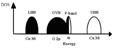
Figure 1: Schematic band structure (density of states (DOS)) of the doped cuprates. LHB and UHB are the lower and upper Habbard bands, respectively, OVB is the oxygen valence band, $P$-band marks the polaronic band, $\varepsilon_{F}$ is the Fermi energy.

III.1 A. Non-pairing polaronic pseudogap

When the energy band of polarons is formed in the CT gap of the cuprates, the states of quasi-free hole carriers in the oxygen valence band become the excited states of a polaron. The Fermi level of polarons $\varepsilon_{F}$ lies inside the CT gap and the threshold energy for photoexcitation of a hole carrier from the polaronic state to a free hole state is given by

$$\Delta\varepsilon_{F}=\varepsilon_{F}^{f}-\varepsilon_{F},$$ (11)

where $\varepsilon_{F}^{f}=\hbar^{2}(3\pi^{2}n)^{2/3}/2m^{*}$ is the Fermi energy of quasi-free hole carriers, $m^{*}$ is the effective mass of these carriers.

The polaronic effects are caused by the unconventional electron-phonon interactions and result in lowering the electronic energy (i.e., the Fermi level or chemical potential $\mu_{F}$ is shifted) by an amount $\Delta\varepsilon_{F}$ and the suppression of the density of states at the Fermi surface of quasi-free electrons (or holes). The so-called non-pairing pseudogap is opened on the former Fermi surface due to the polaronic shift of the electronic states of free carriers. As a result, a large Fermi surface of quasi-free carriers transforms into a small polaronic Fermi surface. Therefore, the excitation energy $\Delta\varepsilon_{F}$ of polarons is manifested in the single-particle spectrum of doped high-$T_{c}$ cuprates as the suppression of the density of states (DOS) at the Fermi level $\varepsilon^{f}_{F}$ and as the non-pairing polaronic pseudogap. As the doping (or $n$) is increased, the Coulomb repulsion between polarons increases and the binding energy $E_{p}$ of polarons decreases, so that the polaronic effect weakens and disappears in the overdoped region. Indeed, the binding energies of polarons $E_{p}=0.12$ eV and $E_{p}=0.06$ eV were observed experimentally in the underdoped and optimally doped cuprates, respectively 93 . One can expect that the dissociation of large polarons due to the Coulomb repulsion between them at short distances occurs at some critical doping level $x=x_{p}$. At $x<x_{p}$, the threshold energy for the thermal excitation of a carrier from the polaronic state to a free-carrier state or for the thermal dissociation of a large polaron can be approximately defined as

$$\Delta_{p}=E_{p}-E_{c},$$ (12)

where $E_{c}=e^{2}/\varepsilon_{0}a_{p}$ is the Coulomb interaction energy between two large polarons, $a_{p}=(3/4\pi n_{a}x)^{1/3}$ is the mean distance between these polarons.

According to the above considerations, depending on the excitation ways, the non-pairing polaronic pseudogap can be determined either from Eq. (11) or from Eq. (12). A better way to define the doping-dependent polaronic pseudogap might be the latter result, Eq. (12), which provides useful information about the characteristic crossover temperature associated with this pseudogap. To evaluate the energy scales of such a pseudogap in underdoped cuprates LSCO, we use Eq. (12) and choose the parameters as $x=0.12$, $\varepsilon_{0}=30$ 89 , $n_{a}\simeq 5.3\cdot 10^{21}\rm{cm^{-3}}$ and $E_{p}\simeq 0.135$ eV. Then we obtain $\Delta_{p}\approx 0.068$ eV, which is in fair agreement with the temperature-independent pseudogap observed experimentally in underdoped LSCO at $500-600\rm{cm^{-1}}$ ($0.06-0.072$ eV) 43 . By taking the parameters $x=0.087$, $\varepsilon_{0}=30$ 89 ; 90 , $n_{a}\approx 10^{22}\rm{cm^{-3}}$ and $E_{p}\simeq 0.143$ eV for YBCO, we find $\Delta_{p}\simeq 0.069$ eV, which is also close to the observed value of the pseudogap $\Delta_{p}\simeq 0.07$ eV in underdoped YBCO 112 . The origin of the large pseudogap ($\Delta_{PG}\sim 0.1$ eV) observed in all underdoped cuprates is most likely associated with the formation of the non-pairing polaronic pseudogap. According to Eq. (12), the polaronic pseudogap decreases with increasing $x$ and disappears at $x=x_{p}$ in accordance with experimental findings 52 ; 53 ; 55 . The pseudogap crossover temperature $T_{p}$ decreases with increasing $x$ and the quantum criticality (quantum phase transition) occurs at some critical doping at which $T_{p}$ goes to zero near a quantum critical point (QCP), $x_{QCP}=x_{p}$ where the breakdown of the usual Fermi-liquid and BCS pairing theories occurs 61 . In the overdoped regime, a large Fermi surface transforms into a small polaronic Fermi surface at $x<x_{QCP}$. This formerly predicted Fermi surface transformation at a QCP 62 was discovered later experimentally 113 . We now consider the doping dependences of the pseudogap crossover temperature $T_{p}(x)=\Delta_{p}(x)/k_{B}$ in various high-$T_{c}$ cuprates. In so doing, we show that the different binding energies $\Delta_{p}$ of polarons determine the different positions of the QCP found from the condition $\Delta_{p}(x)=0$ in LSCO, YBCO and Bi-2212 systems.

III.2 1. Pseudogap phase boundary ending at the quantum critical point $x_{p}\lesssim 0.22$ in LSCO

Various experiments indicate 52 that the unusual and usual metallic states of underdoped to overdoped cuprates above $T_{c}$ are separated by the pseudogap phase boundary or pseudogap crossover line which intersects the superconducting dome and reaches $T=0$ at some critical doping level (i.e., at a QCP).

Figure 2: The doping dependence of the pseudogap crossover temperature $T_{p}$ (solid line) calculated using Eq. (12) at $E_{p}=0.053$ eV, $\varepsilon_{0}=46$ and $n_{a}\simeq 5.3\cdot 10^{21}\rm{cm^{-3}}$. For comparison experimental results (open circles and black squares) corresponding to the openning of the pseudogap in LSCO have been taken from 52 . $T_{c}$ is the critical superconducting transition temperature observed in various experiments.

In particular, the QCP ($x=x_{p}$) in LSCO lies in the doping range $0.20<x<0.24$ 52 ; 114 . By taking $E_{p}\simeq(0.095-0.10)$ eV, $\varepsilon_{0}=30$ and $n_{a}\simeq 5.3\cdot 10^{21}\rm{cm^{-3}}$ (at $V_{a}=190{\AA}$) for LSCO, we obtain $x_{p}\simeq 0.20-0.24$ in accordance with these experimental findings. In Fig. 2, the calculated doping dependence of the polaronic pseudogap crossover temperature $T_{p}(x)$ is compared with the pseudiogap crossover temperature measured on LSCO 52 . As can be seen in Fig. 2, there is a fair agreement between the calculated curve $T_{p}(x)$ and experimental results for $T_{PG}\simeq E_{g}/k_{B}$ in LSCO, where $E_{g}$ is the energy scale of a pseudogap 52 . The transformation of the large Fermi surface of quasi-free carriers to small Fermi surface of large polarons occurs at the QCP located at $x_{QCP}=x_{p}\lesssim 0.22$ above which the Fermi surface of LSCO is in its pristine large Fermi surface state.

III.3 2. Pseudogap phase boundary ending at the quantum critical point $x_{p}\simeq 0.20$ in YBCO

In YBCO the doping-dependent pseudogap determined by using different experimental techniques decreases with increasing $x$ and tends to zero as $x\longrightarrow x_{QCP}\simeq 0.19$ 52 ; 53 or as $x\longrightarrow x_{QCP}\simeq 0.22$ 55 .

Figure 3: The doping dependence of the pseudogap crossover temperature $T_{p}$ (solid line) calculated using Eq. (12) at $E_{p}\simeq 0.142$ eV, $\varepsilon_{0}=22$ and $n_{a}\simeq 1.2\cdot 10^{22}\rm{cm^{-3}}$. For comparison experimental results (open circles, open squares and crosses) corresponding to the openning of the pseudogap in YBCO have been taken from 52 . $T_{c}$ is the experimental values of the critical superconducting transition temperature 52 .

If we take $E_{p}\simeq 0.142$ eV, $\varepsilon_{0}=22$ and $n_{a}=1.2\cdot 10^{22}\rm{cm^{-3}}$ for YBCO, we find from the condition $\Delta_{p}(x)=0$ somewhat different position of the QCP at $x=x_{p}\simeq 0.20$ located between the above experimental values of $x_{QCP}\simeq 0.19$ and $x_{QCP}\simeq 0.22$. In this system the transformation of the large Fermi surface of quasi-free carriers to small Fermi surface of large polarons occurs at the QCP located around $x_{p}\simeq 0.20$, which separates two types of Fermi-liquids (i.e., usual Fermi-liquid and polaronic Fermi-liquid).

III.4 3. Pseudogap phase boundary ending at the quantum critical point $x_{p}\gtrsim 0.22$ in Bi-2212

Experimental results 52 ; 115 provide evidence for the existence of a finite pseudogap at around $x\simeq 0.22$ in the overdoped system Bi-2212. Apparently, the QCP in this system is located at $x\gtrsim 0.22$. By taking the parameters $E_{p}\simeq 0.133$ eV, $\varepsilon_{0}=25$ and $n_{a}=1.3\cdot 10^{22}\rm{cm^{-3}}$ for Bi-2212, we find $x_{QCP}=x_{p}\gtrsim 0.22$ (Fig. 4) in accordance with the experimental results 115 . It follows that the transformation of the large Fermi surface of quasi-free carriers to small Fermi surface of large polarons in Bi-2212 occurs at the QCP located at $x_{p}\gtrsim 0.22$. We see that each of the cuprate superconductor is characterized by the distinct pseudogap phase boundary ending at a specific QCP where Fermi surface reconstruction occurs, somewhere in the overdoped region.

Figure 4: The doping dependence of the pseudogap crossover temperature $T_{p}$ (solid line) calculated using Eq. (12) at $E_{p}\simeq 0.133$ eV, $\varepsilon_{0}=25$ and $n_{a}\simeq 1.3\cdot 10^{22}\rm{cm^{-3}}$. For comparison experimental results (open circles and crosses) corresponding to the openning of the pseudogap in Bi-2212 have been taken from 52 . $T_{c}$ is the experimental values of the critical superconducting transition temperature 52 .

III.5 B. BCS-like pairing pseudogap

The formation of large strongly overlapping Cooper pairs and the superfluidity of such fermionic Cooper pairs in weak-coupling BCS superconductors are assumed to occur at the same temperature $T_{c}$. However, the situation is completely different in more complex systems, in particular, in high-$T_{c}$ cuprates in which the BCS-type Cooper pairing of fermionic quasiparticles without superconductivity can occur above $T_{c}$ and the superfluidity of preformed Cooper pairs becomes possible only at $T_{c}$. In this case, one expects a significant suppression of the density of states at the Fermi surface above $T_{c}$ in the normal state. This so-called BCS-like pairing pseudogap regime extends up to a crossover temperature $T^{*}=T_{F}>T_{c}$ 21 ; 50 . Because the unconventional and more effective electron-phonon interactions are believed to be responsible for the BCS-like pairing correlation above $T_{c}$ and the formation of incoherent (non-superconducting) Cooper-like polaron pairs in the normal state of underdoped, optimally doped and moderately overdoped cuprates. Actually, these high-$T_{c}$ cuprates are unusual metals and have a well-defined and large Fermi surface as follows from ARPES data 43 ; 45 .

The symmetry of the BCS-like pairing pseudogap is still one of the most controversial issues in the physics of high-$T_{c}$ cuprates. Although some experimental observations advocate in favor of a $d$-wave symmetry (see Ref. 116 ), many other experiments 117 ; 118 ; 119 ; 120 closely trace a $s$-wave pairing gap and are incompatible with a $d$-wave pairing symmetry. Further, the $c$-axis bicrystal twist Josephson junction and natural cross-whisker junction experiments provide strong evidence for a $s$-wave pairing gap in high-$T_{c}$ cuprates 121 ; 122 . Müller has argued 123 that a $s$-wave pairing state may, in fact, exist in the bulk of high-$T_{c}$ cuprates. Therefore, we take the view that for high-$T_{c}$ cuprates, the $s$-wave BCS-like pairing state is favored in the bulk and the $s$-wave BCS-like pairing pseudogap could originate from unconventional electron-phonon interactions and carry the physics of the novel BCS-like pairing effects above $T_{c}$.

The high-$T_{c}$ cuprates with low Fermi energies ($\varepsilon_{F}\simeq 0.1-0.3$ eV 44 ; 124 ) and high-energy optical phonons ($\hbar\omega_{0}=0.05-0.08$ eV 81 ; 89 ; 124 ) are in the nonadiabatic regime (i.e., the ratio $\hbar\omega_{0}/\varepsilon_{F}$ is no longer small). For these reasons, the BCS-Eliashberg theory turned out to be inadequate for the description of the formation of unconventional Cooper pairs in high-$T_{c}$ cuprates, where the polaronic effects seem to be important and control the new physics of these systems. In hole-doped cuprates, the new situation arises when the polaronic effects exist and the attractive interaction mechanism (e.g., due to exchange of static and dynamic phonons) between the carriers operating in the energy range $\{-(E_{p}+\hbar\omega_{0}),(E_{p}+\hbar\omega_{0})\}$ is much more effective than in the simple BCS picture. Therefore, the BCS pairing theory should be modified to include polaronic effects. In the case of high-$T_{c}$ cuprates the unusual form of BCS-like pairing theory can describe the formation of polaronic Cooper pairs above $T_{c}$ naturally.

By applying the modified BCS formalism to the interacting Fermi-gas of polarons, we can write the Hamiltonian of this systems with the pair interaction in the form

$$H_{F}=\sum_{k\sigma}\xi(k)a^{+}_{\vec{k}\sigma}a_{\vec{k}\sigma}+\sum_{\vec{k}\vec{k^{\prime}}}V_{p}(\vec{k},\vec{k^{\prime}})a^{+}_{\vec{k}\uparrow}a^{+}_{-\vec{k}\downarrow}a_{-\vec{k^{\prime}}\downarrow}a_{\vec{k^{\prime}}\uparrow},$$

where $\xi(k)=\varepsilon(k)-\varepsilon_{F}$ is the energy of polarons measured from the Fermi energy $\varepsilon_{F}$, $\varepsilon(k)={\hbar}^{2}k^{2}/2m_{p}$, $a^{+}_{{\vec{k}\sigma}}(a_{\vec{k}\sigma})$ is the creation (annihilation) operator for a polaron having momentum $\vec{k}$ and spin projection $\sigma$ ($=\uparrow$ or $\downarrow$), $V_{p}(\vec{k},\vec{k^{\prime}})$ is the pair interaction potential (which has both an attractive and a repulsive part) between large polarons.

The ground state energy of the interacting many-polaron system is calculated by using the model Hamiltonian (III.5). One can assume that the deviations of the products of operators $a^{+}_{\vec{k^{\prime}}\uparrow}$$a^{+}_{-\vec{k^{\prime}}\downarrow}$ and $a_{-\vec{k^{\prime}}\downarrow}$$a_{\vec{k}\uparrow}$ in Eq. (III.5) from their average values $<a^{+}_{\vec{k^{\prime}}\uparrow}a^{+}_{-\vec{k^{\prime}}\downarrow}>$ and $<a_{-\vec{k^{\prime}}\downarrow}a_{\vec{k}\uparrow}>$ are small. Then one pair of operators, $a_{-\vec{k^{\prime}}\downarrow}$$a_{\vec{k}\uparrow}$ or $a^{+}_{\vec{k^{\prime}}\uparrow}$$a^{+}_{-\vec{k^{\prime}}\downarrow}$, can be replaced by its average value. We can write further the identity, following Tinkham 125 , in the form

$$a_{-\vec{k}\downarrow}a_{\vec{k}\uparrow}=F_{\vec{k}}+(a_{-\vec{k}\downarrow}a_{\vec{k}\uparrow}-F_{\vec{k}}),$$ (14)

where $F_{\vec{k}}=<a_{-\vec{k}\downarrow}a_{\vec{k}\uparrow}>$. This is a mean-field approximation and the quantity in the bracket in Eq. (14) is a small fluctuation term. Substituting Eq. (14) and its Hermitian conjugate into the Hamiltonian (III.5) and dropping the term $\sum_{\vec{k},\vec{k^{\prime}}}V_{p}(\vec{k},\vec{k^{\prime}})(a^{+}_{\vec{k^{\prime}}\uparrow}a^{+}_{-\vec{k^{\prime}}\downarrow}-F^{*}_{\vec{k^{\prime}}})(a_{-\vec{k}\downarrow}a_{\vec{k}\uparrow}-F_{\vec{k}}),$ which is the second-order in the fluctuations and is assumed to be very small, the model mean-field Hamiltonian can be written as

$$H_{F}=\sum_{\vec{k}\sigma}\xi(k)a^{+}_{\vec{k}\sigma}a_{\vec{k}\sigma}+$$

$$+\sum_{\vec{k},\vec{k^{\prime}}}V_{p}(\vec{k},\vec{k^{\prime}})[a^{+}_{\vec{k^{\prime}}\uparrow}a^{+}_{-\vec{k^{\prime}}\downarrow}F_{\vec{k}}+a_{\vec{-k}\downarrow}a_{\vec{k}\uparrow}F^{*}_{\vec{k^{\prime}}}-F^{*}_{\vec{k^{\prime}}}F_{\vec{k}}].$$ (15)

Now, we introduce the gap function (or order parameter)

$$\Delta_{F}(\vec{k})=-\sum_{k^{\prime}}V_{p}(\vec{k},\vec{k^{\prime}})<a_{-\vec{k^{\prime}_{\downarrow}}}a_{\vec{k^{\prime}_{\uparrow}}})>=-$$

$$-\sum_{\vec{k^{\prime}}}V_{p}(\vec{k},\vec{k^{\prime}})F_{\vec{k^{\prime}}}.$$ (16)

The function $\Delta_{F}(\vec{k})$ and the Hermitian conjugate function $\Delta^{*}_{F}(\vec{k})$ can be chosen as the real functions 126 . Substituting these functions into Eq. (III.5), we obtain the following resulting Hamiltonian:

$$H_{F}=\sum_{\vec{k}\sigma}\xi(k)\left[a^{+}_{\vec{k}\uparrow}a_{\vec{k}\uparrow}+a^{+}_{-\vec{k}\downarrow}a_{-\vec{k}\downarrow}\right]-$$

$$-\sum_{\vec{k}}\Delta_{F}(\vec{k})\left[a^{+}_{\vec{k}}a^{+}_{-\vec{k}}+a_{-\vec{k}}a_{\vec{k}}-F^{*}_{\vec{k}}\right].$$ (17)

The Hamiltonian (III.5) is diagonalized by using the Bogoliubov transformation:

$$a_{\vec{k}\uparrow}=u_{k}b_{\vec{k}\uparrow}+v_{k}b^{+}_{-\vec{k}\downarrow},\quad a_{-\vec{k}\downarrow}=u_{k}b_{-\vec{k}\downarrow}-v_{k}b^{+}_{\vec{k}\uparrow}$$

$$a^{+}_{\vec{k}\uparrow}=u_{k}b^{+}_{\vec{k}\uparrow}+v_{k}b_{-\vec{k}\downarrow},\quad a^{+}_{-\vec{k}\downarrow}=u_{k}b^{+}_{-\vec{k}\downarrow}-v_{k}b_{\vec{k}\uparrow},$$ (18)

where $b^{+}_{\vec{k}}(b_{\vec{k}})$ is the new creation (annihilation) operator for a Fermi quasiparticle, $u_{k}$ and $v_{k}$ are real functions satisfying the condition

$$u^{2}_{k}+v^{2}_{k}=1.$$ (19)

The new operators $b_{\vec{k}\sigma}$ and $b^{+}_{\vec{k}\sigma}$ just as the old operators $a_{\vec{k}\sigma}$ and $a^{+}_{\vec{k}\sigma}$ satisfy the anticommutation relations of Fermi operators:

$$[b_{\vec{k}\sigma},b_{\vec{k}^{\prime}\sigma^{\prime}}]=[b^{+}_{\vec{k}\sigma},b^{+}_{\vec{k}^{\prime}\sigma^{\prime}}]=0,[b_{\vec{k}\sigma},b^{+}_{\vec{k}^{\prime}\sigma^{\prime}}]=\delta_{\vec{k}\vec{k}^{\prime}}\delta_{\sigma\sigma^{\prime}}.$$

Substituting Eq. (III.5) into Eq. (III.5) and taking into account Eq. (19) and Eq.(III.5), we obtain

$$H_{F}=\sum_{\vec{k}}\Bigg{\{}\left[2\xi(k)v^{2}_{k}-2\Delta_{F}(\vec{k})u_{k}v_{k}\right]+$$

$$+\left[\xi(k)(u^{2}_{k}-v^{2}_{k})+2\Delta_{F}(\vec{k})u_{k}v_{k}\right]$$

$$\times\left(b^{+}_{\vec{k}\uparrow}b_{\vec{k}\uparrow}+b^{+}_{-\vec{k}\downarrow}b_{-\vec{k}\downarrow}\right)+$$

$$+\left[2\xi(k)u_{k}v_{k}-\Delta_{F}(\vec{k})(u^{2}_{k}-v^{2}_{k})\right]$$

$$\times(b^{+}_{\vec{k}\uparrow}b^{+}_{-\vec{k}\downarrow}+b_{-\vec{k}\downarrow}b_{\vec{k}\uparrow})+F^{*}_{\vec{k}}\Delta_{F}(\vec{k})\Bigg{\}}.$$ (21)

We now choose $u_{k}$ and $v_{k}$ so that they are satisfied the condition

$$2\xi(k)u_{k}v_{k}-\Delta_{F}(\vec{k})(u^{2}_{k}-v^{2}_{k})=0.$$ (22)

Then the Hamiltonian (III.5) has the diagonal form and it includes the terms of the ground-state energy $E_{0}$ and the energy $E(\vec{k})$ of quasiparticles

$$H_{F}=E_{0}+\sum_{\vec{k}}E(\vec{k})(b^{+}_{\vec{k}\uparrow}b_{\vec{k}\uparrow}+b^{+}_{-\vec{k}\downarrow}b_{-\vec{k}\downarrow}),$$ (23)

where

$$E_{0}=\sum_{\vec{k}}\left[2\xi(k)v^{2}_{k}-2\Delta_{F}(\vec{k})u_{k}v_{k}+F^{*}_{\vec{k}}\Delta_{F}(\vec{k})\right],$$ (24)

$$E(\vec{k})=\xi(k)(u^{2}_{k}-v^{2}_{k})+2\Delta(\vec{k})u_{k}v_{k}.$$ (25)

As can be seen from Eq. (23), the Hamiltonian (III.5) is reduced to the Hamiltonian of an ideal gas of non-interacting fermionic quasiparticles. Combining Eq. (19) and Eq. (22), and solving the quadratic equation, we have

$$u^{2}_{k}=\frac{1}{2}\left[1+\frac{\xi(k)}{E(\vec{k})}\right],\quad v^{2}_{k}=\frac{1}{2}\left[1-\frac{\xi(k)}{E(\vec{k})}\right].$$ (26)

Substituting Eqs. (24), (25) and (26) into Eq. (23), we obtain

$$H_{F}=\sum_{\vec{k}}\Bigg{\{}\left[\xi(k)-E(\vec{k})+F^{*}_{\vec{k}}\Delta_{F}(\vec{k})\right]+$$

$$+E(\vec{k})\left[b^{+}_{\vec{k}\uparrow}b_{\vec{k}\uparrow}+b^{+}_{-\vec{k}\downarrow}b_{-\vec{k}\downarrow}\right]\Bigg{\}}.$$ (27)

For the unconventional pairing interactions, it is argued 21 (see also Ref. 26 ) that the pseudogap phase has a BCS-like dispersion given by $E(\vec{k})=\sqrt{\xi^{2}(k)+\Delta^{2}_{F}(\vec{k})}$, but the BCS-like gap $\Delta_{F}(\vec{k})$ is no longer superconducting order parameter and appears on the Fermi surface at a characteristic temperature $T^{*}$, which represents the onset temperature of the Cooper pairing of fermionic quasiparticles above $T_{c}$.

We can now determine the BCS-like energy gap $\Delta_{F}(\vec{k})$ and related normal state pseudogap crossover temperature $T^{*}$. After replacing the $a_{\vec{k}\sigma}$ operators by the $b_{\vec{k}\sigma}$ operators and dropping the off-diagonal operators $b_{-\vec{k}^{\prime}_{\downarrow}}b_{\vec{k}^{\prime}_{\uparrow}}$ and $b^{+}_{\vec{k}^{\prime}_{\uparrow}}b^{+}_{-\vec{k}^{\prime}_{\downarrow}}$, which do not contribute to the average value of the product of operators $a_{-\vec{k}^{\prime}_{\downarrow}}a_{\vec{k}^{\prime}_{\uparrow}}$, the gap function or order parameter $\Delta_{F}(\vec{k})$ is given by

$$\Delta_{F}(\vec{k})=-\sum_{\vec{k}^{\prime}}V_{p}(\vec{k},\vec{k}^{\prime})(1-$$

$$-b^{+}_{\vec{k}^{\prime}\uparrow}b_{\vec{k}^{\prime}\uparrow}-b^{+}_{-\vec{k}^{\prime}\downarrow}b_{-\vec{k}^{\prime}\downarrow}).$$ (28)

This BCS-like energy gap exists in the excitation spectrum $E(\vec{k})$ of fermionic quasiparticles. Therefore, the number of such quasiparticles populating the state $\vec{k}$ at the temperature $T$ is

$$\langle b^{+}_{\vec{k}\sigma}b_{\vec{k}\sigma}\rangle=f(E(\vec{k},T))=\left[\exp\left(\frac{E(\vec{k})}{k_{B}T}\right)+1\right]^{-1}.$$ (29)

Using this relation the gap equation (III.5) can be written as

$$\Delta_{F}(\vec{k},T)=-\sum_{\vec{k}^{\prime}}V_{p}(\vec{k},\vec{k}^{\prime})u_{\vec{k}^{\prime}}v_{\vec{k}^{\prime}}\big{[}1-2f(\vec{k}^{\prime},T)].$$ (30)

At $T=0$ there are no quasiparticles, so that $f(E(\vec{k},T))=0$.

Thus, the temperature-dependent BCS-like gap equation is given by

$$\Delta_{F}(\vec{k},T)=-\sum\limits_{\vec{k}^{\prime}}V_{p}(\vec{k},\vec{k}^{\prime})\frac{\Delta_{F}(\vec{k}^{\prime},T)}{2E(\vec{k}^{\prime},T)}\tanh\frac{E(\vec{k}^{\prime},T)}{2k_{B}T}.$$ (31)

Further we use the model potential which may be chosen as

$$V_{p}(\vec{k},\vec{k}^{\prime})=\left\{\begin{array}[]{lll}V_{c}-V_{ph}&\textrm{for}\>|\xi(k)|,\>|\xi(k^{\prime})|\leq\varepsilon_{A},\\ V_{c}&\textrm{for}\>\varepsilon_{A}\leq|\xi(k)|,\>|\xi(k^{\prime})|<\varepsilon_{c},\\ 0&\>\textrm{otherwise},\end{array}\right.$$ (35)

where $\varepsilon_{A}=E_{p}+\hbar\omega_{0}$ is the cutoff parameter for the attractive part of the potential $V_{p}(\vec{k},\vec{k}^{\prime})$, $V_{ph}$ is the phonon-mediated attractive interaction potential between two polarons, $V_{c}$ is the repulsive Coulomb interaction potential between these carriers, $\varepsilon_{c}$ is the cutoff parameter for the Coulomb interaction.

Using the model potential Eq. (35) and replacing the sum over $\vec{k^{\prime}}$ by an integral over $\varepsilon$ in Eq. (31), we obtain the following BCS-like equation for determining the energy gap (or pseudogap), $\Delta_{F}(T)$ and the mean-field pairing temperature $T^{*}(>T_{c})$:

$$\frac{1}{\lambda^{*}_{p}}=\int\limits_{0}^{\varepsilon_{A}}\frac{d\xi}{\sqrt{\xi^{2}+\Delta^{2}_{F}(T)}}\tanh{\frac{\sqrt{\xi^{2}+\Delta^{2}_{F}(T)}}{2k_{B}T}},$$ (36)

where $\lambda^{*}_{p}=D_{p}(\varepsilon_{F})\tilde{V}_{p}$ is the effective BCS-like coupling constant for pairing polarons, $D_{p}(\varepsilon_{F})$ is the DOS at the polaronic Fermi level, $\tilde{V}_{p}=V_{ph}-\tilde{V}_{c}$ is the effective pairing interaction potential between two large polarons, $\tilde{V}_{c}=V_{c}/[1+D_{p}(\varepsilon_{F})V_{c}\ln(\varepsilon_{c}/\varepsilon_{A})]$ is the screened Coulomb interaction between these polarons.

We can find the temperature-dependent pseudogap $\Delta_{F}(T)$ and the pseudogap formation temperature $T^{*}$ from Eq. (36) at $\lambda_{p}^{*}<1$. At $T=0$, solving Eq. (36) for $\Delta_{F}$, we have

$$\Delta_{F}=\Delta_{F}(0)=\frac{E_{p}+\hbar\omega_{0}}{\sinh[1/\lambda_{p}^{*}]}.$$ (37)

Evidently, as $T\rightarrow T^{*}$, the BCS-like pairing gap $\Delta_{T}(T)$ tends to zero and the Eq. (36) becomes

$$\frac{1}{\lambda_{p}^{*}}=\int^{\varepsilon_{A}}_{0}\frac{d\xi}{\xi}\tanh\frac{\xi}{2k_{B}T^{*}}=\int^{1}_{0}\frac{dy}{y}\tanh y+$$

$$+\int^{y^{*}}_{1}\frac{dy}{y}\tanh y,$$ (38)

where $y^{*}=\varepsilon_{A}/2k_{B}T^{*}$.

In order to evaluate the second integral in Eq. (III.5), it can be written in the form

$$\int_{1}^{y^{*}}\frac{dy}{y}\tanh y=C_{2}+\int_{1}^{y^{*}}\frac{dy}{y}=C_{2}+\ln y^{*},$$ (39)

from which $C_{2}$ is determined for a given value of $y^{*}$.

Substituting this expression into Eq. (III.5), we have the following equation:

$$\frac{1}{\lambda_{p}^{*}}=0.909675+C_{2}+\ln y^{*}=\ln(C^{*}\frac{\varepsilon_{A}}{k_{B}T^{*}}),$$ (40)

where $C^{*}=0.5\exp[C_{2}+0.909675]$.

Thus, the onset temperature of the precursor Cooper pairing of polarons is determined from the relation

$$k_{B}T^{*}=C^{*}(E_{p}+\hbar\omega_{0})exp\big{[}-\frac{1}{\lambda^{*}_{p}}].$$ (41)

As seen from this equation, the BCS-like mean-field pairing temperature $T^{*}$ depends on the phonon energy $\hbar\omega_{0}$ and on the polaron binding energy $E_{p}$. The important point is that the relation (41) is the general expression for the characteristic temperature $T^{*}(\geq T_{c})$ of a BCS-like phase transition. The expression (41) applies equally to the usual BCS-type superconductors (e.g., heavily overdoped cuprates are such systems) and to the unconventional (non-BCS-type) superconductors, such as underdoped, optimally doped and moderately overdoped high-$T_{c}$ cuprates. From this expression it follows that the usual BCS picture ($T_{c}=T^{*}$) as the particular case is recovered in the weak electron-phonon coupling regime (i.e., in the absence of polaronic effects, $E_{p}=0$) and the prefactor $E_{p}+\hbar\omega_{0}$ in Eq. (41) is replaced by $\hbar\omega_{0}$ for heavily overdoped cuprates.

The calculated values of the parameters $C^{*}$ and $\lambda^{*}_{p}$ for different values of $(E_{p}+\hbar\omega_{0})/k_{B}T^{*}$ are presented in Table II. Combining Eqs. (37) and (41), we find the BCS-like ratio

$$\frac{2\Delta_{F}}{k_{B}T^{*}}=\frac{4}{C^{*}[1-\exp(-2/\lambda^{*}_{p})]},$$ (42)

which is characteristic quantity measured in experiments.

Table 2: Calculated values of the prefactor $C^{*}$ and BCS-like coupling constant $\lambda_{p}^{*}$ in Eq. (41) at different values of $(E_{p}+\hbar\omega_{0})/k_{B}T^{*}$.

$\displaystyle{\frac{E_{p}+\hbar\omega_{0}}{k_{B}T^{*}}}$	$C^{*}$	$\lambda_{p}^{*}$
3.00	1.16304	0.80023
4.00	1.14238	0.65815
5.00	1.13646	0.57559
6.00	1.13468	0.52135
7.00	1.13413	0.48268
8.00	1.13395	0.45348
9.00	1.13389	0.43050
10.00	1.13388	0.41182
15.00	1.13387	0.35290
20.00	1.13387	0.32037

III.6 1. Comparison with experiments

The smooth evolution of the energy gap observed in the tunneling and ARPES spectra of high-$T_{c}$ cuprates with lowering the temperature from a pseudogap state above the critical temperature $T_{c}$ to a superconducting state below $T_{c}$, has been poorly interpreted previously as the evidence that the pseudogap must have the same origin as the superconducting order parameter, and therefore, must be related to $T_{c}$. According to the tunneling and ARPES data 127 ; 128 , the observed energy gap follows BCS-like gap equation and closes at a temperature well above $T_{c}$, where Cooper pairs disappear. However, these key experimental findings are not indicative yet of the superconducting origin of the BCS-like gap below $T_{c}$, which persists as a pseudogap in the normal state above $T_{c}$. The interpretation of the BCS-like gap below $T_{c}$ as a superconducting order parameter contradicts with other experiments 33 ; 59 ; 60 in which the superconducting transition at $T_{c}$ is $\lambda$-like but not BCS-like transition. Actually, the anomalous behaviors of the gap $\Delta_{0}$ and ratio $2\Delta_{0}/k_{B}T_{c}$ (where $\Delta_{0}$ is the energy gap observed experimentally and often described as the superconducting order parameter in various high-$T_{c}$ cuprates without any justification) cast a doubt on the BCS-like pairing theory as a theory of unconventional cuprate superconductivity. The numerical solution of Eq. (36) determines the temperature dependence of a BCS-like gap, which extends to the precursor Cooper pairing regime above $T_{c}$ 128 . In high-$T_{c}$ cuprates the energy of the effective attraction between polaronic carriers at their Cooper pairing is determined as $\varepsilon_{A}=E_{p}+\hbar\omega_{0}$. These high-$T_{c}$ materials are characterized by optical phonons with energies in the range 0.03-0.08 eV 89 ; 124 . The binding energy of large polarons $E_{p}$ varies from 0.05 eV (at $\varepsilon_{\infty}=5$ and $\eta=0.04$) to 0.14 eV (at $\varepsilon_{\infty}=3$ and $\eta=0.04$). For $\lambda^{*}_{p}\lesssim 0.5$ the prefactor in Eq. (41) is given by $C\simeq 1.134$ (see Table II). The values of $T^{*}$ determined from this equation are compared with the experimental values of $T^{*}$ presented in Table III for underdoped (UD), optimally doped (OPD) and overdoped (OD) cuprates. As a result, we obtained the values of $\varepsilon_{A}$ and $\lambda^{*}_{p}$ presented in Table III. Then, the values of $\Delta_{F}$ are determined from the relation (37) and presented also in Table III for the comparison with the experimental values of $\Delta_{0}$. Next, the values of the ratio $2\Delta_{F}/k_{B}T_{c}$ are calculated by using the experimental values of $T_{c}$ presented in Table III, while the values of the BCS-like ratio $2\Delta_{F}/k_{B}T^{*}$ are determined from Eq. (42). The calculated and experimental values of the ratios $2\Delta_{F}/k_{B}T_{c}$, $2\Delta_{F}/k_{B}T^{*}$, $2\Delta_{0}/k_{B}T_{c}$ and $2\Delta_{0}/k_{B}T^{*}$ in various high-$T_{c}$ cuprates are presented in Table IV.

Table 3: Theoretical and experimental values of energy gaps ($\Delta_{F}$ and $\Delta_{0}$) and characteristic pseudogap and superconducting transition temperatures ($T^{*}$ and $T_{c}$) in various high-$T_{c}$ cuprate superconductors.

	Theory				Experiment
						43 ; 127
Cuprate	$\varepsilon_{A}$	$\lambda^{*}_{p}$	$\Delta_{F}$,	$T^{*}$,	$T_{c}$,	$\Delta_{0}$,	$T^{*}$,
materials	eV		eV	K	K	eV	K
LSCO UD	0.11	0.352	0.013	84	40	0.016	82
LSCO OD	0.10	0.319	0.009	57	40	0.010	53
Bi-2212 UD	0.13	0.442	0.027	178	82	0.027	180
Bi-2212 OPD	0.14	0.393	0.022	144	88	0.025	142
Bi-2212 OD	0.13	0.378	0.019	121	120	0.020	120
YBa2Cu3O6.95 OPD	0.12	0.377	0.017	111	92	0.020	110
YBa2Cu4O8	0.13	0.467	0.031	200	81	-	200

Table 4: Theoretical and experimental values of the ratios $2\Delta_{F}/k_{B}T_{c}$, $2\Delta_{F}/k_{B}T^{*}$, $2\Delta_{0}/k_{B}T_{c}$, and $2\Delta_{0}/k_{B}T^{*}$ in various cuprate superconductors.

	Theory		Experiment 43 ; 127
Cuprate materials	$\displaystyle{\frac{2\Delta_{F}}{k_{B}T_{c}}}$	$\displaystyle{\frac{2\Delta_{F}}{k_{B}T^{*}}}$	$\displaystyle{\frac{2\Delta_{0}}{k_{B}T_{c}}}$	$\displaystyle{\frac{2\Delta_{0}}{k_{B}T^{*}}}$
LSCO UD	7.536	3.539	9.271	4.522
LSCO OD	5.797	3.534	5.794	4.373
Bi-2212 UD	7.635	3.566	7.632	3.477
Bi-2212 OPD	5.797	3.549	6.584	4.081
Bi-2212 OD	5.373	3.545	5.653	3.863
YBa2Cu3O6.95 OPD	4.285	3.545	5.039	4.214
YBa2Cu4O8	8.875	3.577	-	-

As can be seen from Table III, the difference between $T^{*}$ and $T_{c}$ is large enough in UD cuprates (where $T^{*}/T_{c}\simeq 2.05-2.20$) compared to OD cuprates (where $T^{*}/T_{c}\simeq 1.32-1.46$) and the BCS-like pseudogap regime is extended over a much wider temperature range above $T_{c}$ in UD cuprates than in OD cuprates. Further, both the BCS-like pseudogap $\Delta_{F}$ and the gap $\Delta_{0}$ observed experimentally in various high-$T_{c}$ cuprates scales with $T^{*}$, not with $T_{c}$, i.e., both the $\Delta_{F}$ and the $\Delta_{0}$ are closely related to the characteristic pseudogap temperature $T^{*}$ and not related to $T_{c}$. The unusually large gap values (i.e. $2\Delta_{F}(=\Delta_{0})/k_{B}T_{c}>>3.54-3.58$) observed in various high-$T_{c}$ cuprates (see Table IV) clearly indicate that the BCS-like gap (order parameter) $\Delta_{F}=\Delta_{0}$ appearing at $T^{*}$ is not associated with the superconducting transition at $T=T_{c}$. It follows that the identification of this energy gap by many researchers as a superconducting order parameter ( often called also superconducting gap) in the cuprates, from UD to OD regime is a misinterpretation of such a BCS-like gap. Actually, the single-particle tunneling spectroscopy and ARPES provide information about the excitation gaps at the Fermi surface but fail to identify the true superconducting oreder parameter appearing below $T_{c}$ in non-BCS cuprate superconductors. When polaronic effects cause separation between the two characteristic temperatures $T^{*}$ (the onset of the Cooper pairing) and $T_{c}$ (the onset of the superconducting transition) in these superconductors, both the $s$-wave and the $d$-wave BCS-like pairing theory cannot be used to describe the novel superconducting transition at $T_{c}$. In this case the superconducting order parameter $\Delta_{SC}$ should not be confused with the BCS-like ($s$- or $d$-wave) gap.

III.7 2. Doping dependences of $T^{*}$ and their experimental confirmations in various high-$T_{c}$ cuprates

To determine the characteristic doping dependences of $\Delta_{F}$ and $T^{*}$, we can approximate the DOS at the Fermi level in a simple form

$$D_{p}(\varepsilon_{F})=\left\{\begin{array}[]{lll}1/\varepsilon_{F}&\textrm{for}\>\varepsilon<\varepsilon_{F}\\ 0&\>\textrm{otherwise}.\end{array}\right.$$ (45)

Using this approximation we obtain from Eqs. (37) and (41)

$$\Delta_{F}(x)=\frac{2(E_{p}+\hbar\omega_{0})\exp(-\frac{\hbar^{2}(3\pi^{2}n_{a}x)^{2/3}}{2m_{p}\tilde{V}_{p}})}{[1-\exp(-\frac{\hbar^{2}(3\pi^{2}n_{a}x)^{2/3}}{m_{p}\tilde{V}_{p}})]},$$ (46)

and

$$k_{B}T^{*}(x)=C^{*}(E_{p}+\hbar\omega_{0})exp\big{[}-\frac{\hbar^{2}(3\pi^{2}n_{a}x)^{2/3}}{2m_{p}\tilde{V}_{p}}].$$ (47)

Figure 5: Doping dependence of the characteristic pseudogap temperature $T^{*}$ (solid line) calculated using the Eq. (47) with parameters $E_{p}+\hbar\omega_{0}=0.08$ eV, $m_{p}=1.8m_{e}$, $n_{a}\simeq 5.3\cdot 10^{21}\rm{cm^{-3}}$ and $\tilde{V}_{p}=0.059$ eV. Experimental results for $T^{*}$ have been taken from ARPES (open circles and open square) and tunneling (full triangles) data in LSCO 102 . Black circles are experimental data for $T_{c}$ 102 .

Figure 6: Doping dependence of the characteristic pseudogap temperature $T^{*}$ (solid line) calculated using the Eq. (47) with parameters $E_{p}+\hbar\omega_{0}=0.12$ eV, $m_{p}=2.2m_{e}$, $n_{a}\simeq 1.2\cdot 10^{22}\rm{cm^{-3}}$ and $\tilde{V}_{p}=0.093$ eV. Experimental results for $T^{*}$ in YBCO have been taken from 99 (black circles) and 130 (open circles, triangles and square). Open squares are experimental data for $T_{c}$ 131 .

Figure 7: Doping dependence of the characteristic pseudogap temperature $T^{*}$ (solid line) calculated using the Eq. (47) with parameters $E_{p}+\hbar\omega_{0}=0.098$ eV, $m_{p}=2m_{e}$, $n_{a}\simeq 1.3\cdot 10^{22}\rm{cm^{-3}}$ and $\tilde{V}_{p}=0.125$ eV. Experimental results for $T^{*}$ in Bi-2212 have been taken from 7 (open circles), 132 (open square) and 133 (black squares), 134 (black stars). Open triangles are experimental data for $T_{c}$ 128 .

As seen from Eqs. (46) and (47), both the BCS-like pairing pseudogap $\Delta_{F}$ and the characteristic pseudogap temperature $T^{*}$ has an exponentially increasing dependence on the doping level $x$. Such doping dependences of $\Delta_{F}(x)$ and $T^{*}(x)$ were observed experimentally in high-$T_{c}$ cuprates 7 ; 9 ; 129 . We now compare the calculated doping dependences of $T^{*}$ with experimental results for $T^{*}(x)$ in LSCO, YBCO and Bi-2212. We have found that the calculated results for $T^{*}(x)$ are similar to the experimentally measured doping dependences of $T^{*}$ in these high-$T_{c}$ cuprates, as shown in Figs. 5-7.

III.8 C. Proposed normal-state phase diagrams of the La-, Y- and Bi-based high-$T_{c}$ cuprates

We now construct the unified normal-state phase diagrams of high-$T_{c}$ cuprates in the space of $x$ vs $T$ based on the above theoretical and experimental results. In Figs. 8-10, we summarise characteristic pseudogap temperatures as a function of doping and temperature to demonstrate the existence of two distinct pseudogap regimes above $T_{c}$ and QCP at the end point of the pseudogap phase boundary in LSCO, YBCO and Bi-2212. The key feature of these proposed phase diagrams is the existence of three distinct phase regions (which correspond to three distinct metallic phases) above $T_{c}$, separated by two different pseudogap crossover lines $T^{*}(x)$ and $T_{p}(x)$. In each $T-x$ phase diagram has a very important phase boundary separating two fundamentally different (pseudogap metal and ordinary metal) states of underdoped and optimally doped cuprates. The $T_{p}(x)$ curve (pseudogap phase boundary) crosses the dome-shaped $T_{c}(x)$ curve at around the optimal doping level, and then fall down to $T=0$ at the polaronic QCP, $x=x_{p}$, inside the superconducting phase. Since the discovery of the pseudogap phase boundary 52 ; 62 ; 65 ; 67 , its origin has been under dispute 55 ; 115 ; 135 . The $T-x$ phase diagrams presented in Figs. 8-10 resolve conflicting reports about the fate of the pseudogap phase boundary line discovered experimentally by Loram and Tallon 52 . These phase diagrams clearly demonstrate that the Loram-Tallon line is none other than the polaronic pseudogap crossover line $T_{p}(x)$.

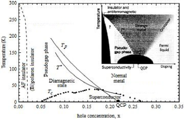
Figure 8: Normal-state phase diagram of LSCO, showing two distinct characteristic pseudogap temperatures $T_{p}$ (solid line which is the same crossover line $T_{p}(x)$ as in Fig. 2) and $T^{*}$ (solid line which is the same crossover line $T^{*}(x)$ as in Fig. 5) and diamagnetism below $T^{*}$, is compared with the other phase diagram 68 (see inset). Black circles are experimental data for $T_{c}$ 102 . The $T_{p}(x)$ line is the pseudogap phase boundary ending at the QCP, $x_{QCP}\lesssim 0.22$. The other line $T^{*}(x)$ is the BCS-like transition (or BCS-like pseudogap crossover) line and merges with the $T_{c}(x)$ line in the overdoped region.

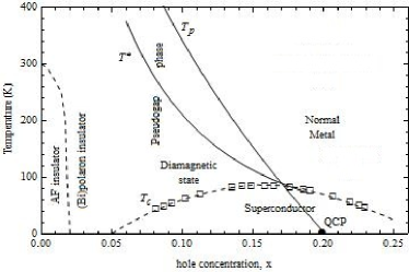
Figure 9: Normal-state phase diagram of YBCO showing two distinct characteristic pseudogap temperatures $T_{p}$ (solid line which is the same crossover line $T_{p}(x)$ as in Fig. 3) and $T^{*}$ (solid line which is the same crossover line $T^{*}(x)$ as in Fig. 6) and diamagnetism below $T^{*}$. Open squares are experimental data for $T_{c}$ 131 . The $T_{p}(x)$ line is the pseudogap phase boundary ending at the QCP, $x_{QCP}\simeq 0.20$. The other line $T^{*}(x)$ is the BCS-like transition (or BCS-like pseudogap crossover) line and merges with the $T_{c}(x)$ line in the overdoped region.

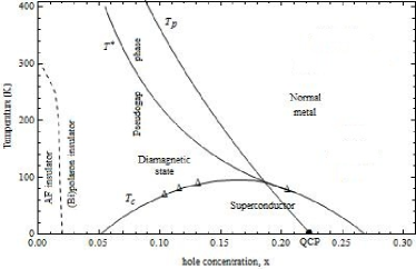
Figure 10: Normal-sate phase diagram of Bi-2212 showing two distinct characteristic pseudogap temperatures $T_{p}$ (solid line which is the same crossover line $T_{p}(x)$ as in Fig. 4) and $T^{*}$ (solid line which is the same crossover line $T^{*}(x)$ as in Fig. 7) and diamagnetism below $T^{*}$. Open triangles are experimental data for $T_{c}$ 128 . The $T_{p}(x)$ line is the pseudogap phase boundary ending at the QCP, $x_{QCP}\gtrsim 0.22$. The other line $T^{*}(x)$ is the BCS-like transition (or BCS-like pseudogap crossover) line and merges with the $T_{c}(x)$ line in the overdoped region.

According to the proposed normal-state phase diagrams of high-$T_{c}$ cuprates, one can observe above $T_{c}$ such properties as the two gap-like features and related abnormal metallic properties, anomalous diamagnetism, from underdoped to overdoped regime, that is, many features that are characteristic of a pseudogap state. In particular, the diamagnetism observed above $T_{c}$ 35 ; 49 is associated with the formation of polaronic Cooper pairs (with zero spin) and would persist up to pseudogap temperature $T^{*}$.

In the underdoped and optimally doped cuprates we have a great variety of experimental evidence that there is a large pristine Fermi surface above the pseudogap crossover line $T_{p}(x)$ but below this line the unusual metallic state is based upon a small polaronic Fermi surface. Further, various experiments and above presented theoretical results indicate that the other pseudogap crossover line $T^{*}(x)$ does not intersect the superconducting dome and smoothly merges into the $T_{c}(x)$ line with overdoping in LSCO, YBCO and Bi-2212. This explains why the pseudogap state was never observed in the overdoped regime except the moderately overdoped region in high-$T_{c}$ cuprates. The smooth merging of $T^{*}(x)$ and $T_{c}(x)$ lines in the overdoped region suggests that cuprates become a conventional superconductor with $T_{c}=T^{*}$. Because the Cooper pairing and Fermi-liquid superconductivity occur at the same temperature $T_{c}$. However, in underdoped and optimally doped (including also slightly overdoped) regimes the BCS-like pseudogap (below $T^{*}$) and the polaronic pseudogap (below $T_{p}$) exist in the normal state of high-$T_{c}$ cuprates. So we have, as a function of $x$ and $T$, another very fundamental BCS-like pseudogap phase boundary: between the state based upon a polaronic Fermi surface and the state where the polarons have already paired up in the BCS regime and there remains only a small collapsed Fermi surface. The pseudogap crossover line $T_{p}(x)$ intersects the $T^{*}(x)$ line and the superconducting dome in the slightly overdoped regime and then ends at a specific QCP in LSCO, YBCO and Bi-2212.

IV IV. PSEUDOGAP EFFECTS ON THE NORMAL-STATE PROPERTIES OF HIGH-$T_{c}$ CUPRATES

The above two distinct pseudogaps, especially BCS-like pairing pseudogap, discovered in underdoped, optimally doped and moderately overdoped cuprates affect the normal-state properties of these high-$T_{c}$ materials and result in the appearance of their anomalous behaviors below the characteristic pseudogap crossover temperatures. Because the pseudogaps have strong effects on the electronic states of the doped high-$T_{c}$ cuprates and manifest themselves both in doping dependences and in temperature dependences of various physical quantities such as the optical, transport, thermodynamic and other properties of these intricate materials. In this section, we discuss the possible effects of the pseudogaps on the normal state properties of underdoped to overdoped cuprates.

IV.1 A. Normal-state charge transport

In the layered cuprates the normal-state in-plane resistivity $\rho(T)$ shows various anomalous behaviors below the crossover temperature $T^{*}$ and above this temperature $\rho(T)$ exhibits a $T$-linear behavior. Below $T^{*}$, $\rho(T)$ deviates either downwards (i.e. $\rho(T)$ shows a bending behavior) or upwards from the high-temperature behavior 43 ; 136 . In particular, $\rho(T)$ in some high-$T_{c}$ cuprates shows a positive curvature in the temperature range $T_{c}<T<T^{*}$ 136 ; 137 and a maximum (i.e. abnormal resistivity peak) between $T_{c}$ and $T^{*}$ 138 ; 139 ; 140 . Sometimes, anomalous resistive transitions (i.e. a sharp drop 141 ; 142 and a clear jump 139 ; 140 in $\rho(T)$) were also observed at $T^{*}$. It is widely believed that the $T$-linear behavior of $\rho(T)$ above $T^{*}$ is also indicative of an unusual property of high-$T_{c}$ cuprate superconductors and is characteristic of the strange metal 35 ; 111 . Some theories of the pseudogap phenomena have attempted to explain the linear temperature dependence of $\rho(T)$ 65 ; 143 ; 144 , but the precise nature of the $T$-linear behavior of $\rho(T)$ in high-$T_{c}$ cuprates remains a complete mystery to these as well as to other existing theories. Further, any microscopic theory that tries to explain the pseudogap effects on the normal-state resistivity of high-$T_{c}$ cuprates must be able to consistently and quantitatively explain not only $T$-linear resistivity above $T^{*}$ but also all the anomalies in $\rho(T)$ observed below $T^{*}$.

In a more realistic model, the charge carriers in polar crystals are scattered by acoustic and optical phonons and these scattering processes are major sources of temperature-dependent resistivity in the cuprates above $T_{c}$ and can describe better the normal-state transport properties. Therefore, we consider here the scattering of charge carriers by the acoustic and optical lattice vibrations, in order to find the variation of the conductivity (resistivity) with the temperature of the crystal. We believe that the in-plane conductivity of underdoped to overdoped cuprates will be associated with the metallic transport of large polarons, bosonic Cooper pairs and polaronic components of such Cooper pairs in the CuO₂ layers. Using the Boltzmann transport equations in the relaxation time approximation, we can obtain appropriate equations for the conductivity of large polarons above $T^{*}$ and for the conductivities of the excited Fermi components of polaronic Cooper pairs and the very bosonic Cooper pairs below $T^{*}$. It is natural to believe that the polaronic carriers and bosonic Cooper pairs are scattered effectively by optical phonons having the specific frequencies $\omega_{0}=\omega_{01}$ and $\omega_{0}=\omega_{02}$, respectively. The total scattering probability of polaronic carriers scattered by acoustic and optical phonons is defined by the sum of two possible scattering probabilities. Above $T^{*}$ the total relaxation time $\tau_{p}(\varepsilon)$ of such carriers having the energy $\varepsilon$ is determined from the relation 145

$$\frac{1}{\tau_{p}(\varepsilon)}=\frac{1}{\tau_{ac}(\varepsilon)}+\frac{1}{\tau_{op}},$$ (48)

where $\tau_{ac}(\varepsilon)=A_{p}/t\sqrt{\varepsilon}$ is the relaxation time of large polarons scattered by acoustic phonons, $\tau_{op}=B_{p}\exp[\hbar\omega_{01}/k_{B}T^{*}t]$ is the relaxation time of such carriers scattered by optical phonons, $A_{p}=\pi\hbar^{2}\rho_{M}\upsilon^{2}_{s}/\sqrt{2}E^{2}_{d}m^{3/2}_{p}k_{B}T^{*}$, $B_{p}=4\sqrt{2}\pi\tilde{\varepsilon}(\hbar\omega_{01})^{3/2}/\omega^{2}_{01}e^{2}\sqrt{m_{p}}$, $t=T/T^{*}$, $\rho_{M}$ is the material density, $\upsilon_{s}$ is the sound velocity.

We now consider the layered cuprate superconductor with a simple ellipsoidal energy surface and the normal-state conductivity of polaronic carriers in the quasi-2D CuO₂ layers (with nonzero thickness). We will take such an approach, since it seems more natural. We further take the components of the polaron mass $m_{p_{1}}=m_{p_{2}}=m_{ab}$ for the $ab$-plane and $m_{p_{3}}=m_{c}$ for the $c$-axis in the cuprates. Then the effective mass $m_{p}$ of polarons in the layered cuprates is $(m^{2}_{ab}m_{c})^{1/3}$.

IV.2 B. Normal-state conductivity of polarons above $T^{*}$

When the electric field is applied in the $x$-direction, the conductivity of polaronic carriers in high-$T_{c}$ materials above $T^{*}$ in the relaxation time approximation is given by

$$\sigma_{p}(T>T^{*})=-\frac{e^{2}}{4\pi^{3}}\int\tau_{p}(\varepsilon)v_{x}^{2}\frac{\partial f_{p}}{\partial\varepsilon}d^{3}k,$$ (49)

where, $f_{p}(\varepsilon)=(e^{(\varepsilon-\mu)/k_{B}T}+1)^{-1}$ is the Fermi distribution function, $\varepsilon=\hbar^{2}k^{2}/2m_{p}$ and $v_{x}=\frac{1}{\hbar}\frac{\partial\varepsilon}{\partial k_{x}}$ are the energy and velocity of polarons, $m_{p}=(m^{2}_{ab}m_{c})^{1/3}$.

In the case of an ellipsoidal energy surface, we make the following transformations similarly to Ref. 146 : $k_{x}=m_{ab}^{1/2}k^{\prime}_{x}$, $k_{y}=m_{ab}^{1/2}k^{\prime}_{y}$, $k_{z}=m_{c}^{1/2}k^{\prime}_{z}$. Then the in-plane and out-of-plane kinetic energies are transformed from $\hbar^{2}(k^{2}_{x}+k^{2}_{y})/2m_{ab}$ and $\hbar^{2}k_{z}^{2}/2m_{c}$ to $(k^{{}^{\prime}2}_{x}+k^{{}^{\prime}2}_{y})/2$ and $\hbar^{2}k^{\prime 2}_{z}/2$ respectively. As a result, average kinetic energy of a carrier over the energy layer $\Delta\varepsilon$ along three directions $k_{x}$, $k_{y}$ and $k_{z}$ is the same and equal to one third of the total energy $\varepsilon$. Therefore, replacing $v_{x}^{2}$ by $\hbar^{2}k^{\prime 2}_{x}/m_{ab}$ and using the relation $d^{3}k=(m^{2}_{ab}m_{c})^{1/3}d^{3}k^{\prime}$, we may write Eq. (49) in the form

$$\sigma_{p}(T>T^{*})=-\frac{e^{2}}{4\pi^{2}}(m^{2}_{ab}m_{c})^{1/2}\int\tau_{p}(\varepsilon)\frac{\hbar^{2}k^{\prime 2}_{x}}{m_{ab}}\frac{\partial f_{p}}{\partial\varepsilon}d^{3}k^{\prime}.$$

Replacing $k^{\prime 2}_{x}$ by $2\varepsilon/3\hbar^{2}$ and using further the carrier density $n$ given by

$$n=\frac{2}{(2\pi)^{3}}\int f_{p}(k)d^{3}k=\frac{(2m_{ab}^{2}m_{c})^{1/2}}{\pi^{2}\hbar^{3}}\int f_{p}(\varepsilon)\varepsilon^{1/2}d\varepsilon,$$

the expression (IV.2) is written as

$$\sigma_{p}(T>T^{*})=\frac{2ne^{2}}{3m_{ab}}\frac{\int\limits_{0}^{\infty}\tau_{p}(\varepsilon)\varepsilon^{3/2}(-\partial f_{p}/\partial\varepsilon)d\varepsilon}{\int\limits_{0}^{\infty}f_{p}(\varepsilon)\varepsilon^{1/2}d\varepsilon}.$$ (52)

When the Fermi energy of large polarons $\varepsilon_{F}$ is much larger than their thermal energy $k_{B}T$, we deal with a degenerate polaronic gas. For a degenerate polaronic Fermi-gas, we have approximately $f_{p}(\varepsilon<\varepsilon_{F})=1$ and $f_{p}(\varepsilon>\varepsilon_{F})=0$. In this case the function $-\partial f_{p}/\partial\varepsilon$ is nonzero only near $\varepsilon=\varepsilon_{F}=\mu_{F}$ and close to the $\delta$-function. Therefore, we may replace $-\partial f_{p}/\partial\varepsilon$ by $\delta(\varepsilon-\varepsilon_{F})$ and the integral in (52) may be evaluated as

$$\int\limits_{0}^{\infty}\tau_{p}(\varepsilon)\varepsilon^{3/2}\left(-\frac{\partial f_{p}}{\partial\varepsilon}\right)d\varepsilon=B_{p}e^{\alpha_{p}/t}\int\limits_{0}^{\infty}\frac{\varepsilon^{3/2}}{1+c_{p}(t)\sqrt{\varepsilon}}\times$$

$$\times\delta(\varepsilon-\varepsilon_{F})d\varepsilon=B_{p}e^{\alpha_{p}/t}\frac{\varepsilon^{3/2}_{F}}{1+c_{p}(t)\sqrt{\varepsilon_{F}}},$$ (53)

where $\alpha_{p}=\hbar\omega_{01}/k_{B}T^{*}$, $c_{p}(t)=(B_{p}/A_{p})te^{\alpha_{p}/t}$.

Using the above property of the Fermi distribution function, the integral in the denominator in Eq. (52) is evaluated as

$$\int\limits_{0}^{\infty}f_{p}(\varepsilon)\varepsilon^{3/2}d\varepsilon=\int\limits_{0}^{\varepsilon_{F}}\varepsilon^{1/2}d\varepsilon=\frac{2}{3}\varepsilon_{F}^{3/2}.$$ (54)

Inserting the relations (IV.2) and (54) into (52), we obtain the normal-state in-plane conductivity

$$\sigma_{ab}(t>1)=\sigma_{p}(t>1)=\frac{ne^{2}B_{p}e^{\alpha_{p}/t}}{m_{ab}(1+c_{p}(t)\sqrt{\varepsilon_{F}})}.$$ (55)

IV.3 C. Normal-state conductivity of the Fermi components of Cooper pairs and the bosonic Cooper pairs below $T^{*}$

As mentioned above, the polaronic carriers in the energy layer of width $\varepsilon_{A}$ around the Fermi surface take part in the BCS-like pairing and form polaronic (bosonic) Cooper pairs. The total number of the excited (dissociated) Fermi components of such Cooper pairs and nonexcited bosonic Cooper pairs is determined from the relation

$$n=n_{p}^{*}+2n_{B}=2\sum_{k}\left[u^{2}_{k}f_{C}(k)+v_{k}^{2}(1-f_{C}(k))\right],$$ (56)

where $n_{p}^{*}=2\sum_{k}u^{2}_{k}f_{C}(k)$ is the number of the excited polaronic components of Cooper pairs, $n_{B}=\sum_{k}v_{k}^{2}(1-f_{C}(k))$ is the number of bosonic Cooper pairs, $f_{C}(k)=f(E(k))=(e^{E/k_{B}T}+1)^{-1}$ is the Fermi distribution function, $E(k)=\sqrt{\xi^{2}(k)+\Delta^{2}_{F}}$, $u_{k}$ and $v_{k}$ are defined in Eq. (26).

The contribution of the excited Fermi components of Cooper pairs to the conductivity in quasi-2D cuprate superconductors below $T^{*}$ in the relaxation time approximation is given by (see Appendix A)

$$\sigma_{p}^{*}(T<T^{*})=-\frac{e^{2}}{8\pi^{3}}\int\tau_{BCS}(\xi)v_{\alpha}^{2}\frac{\xi}{E}\left(1+\frac{\xi}{E}\right)\frac{\partial f_{C}}{\partial E}d^{3}k.$$

When we consider a thin $\rm{CuO_{2}}$ layer of the doped cuprate superconductor with an ellipsoidal energy surface, the expression for $\sigma^{*}_{p}(T<T^{*})$ can be written as

$$\sigma_{p}^{*}(t<1)=\frac{ne^{2}}{3m_{ab}}\times$$

$$\times\frac{\int\limits_{-\varepsilon_{A}}^{\varepsilon_{A}}\tau_{BCS}(\xi+\mu)(\xi+\varepsilon_{F})^{3/2}\frac{\xi}{E}\left(1+\frac{\xi}{E}\right)\left(-\frac{\partial f_{C}}{\partial E}\right)d\xi}{\int\limits_{0}^{\infty}f_{p}(\varepsilon)\varepsilon^{1/2}d\varepsilon}.$$

If we use the property of $\delta$- function $\delta[E(k^{\prime})-E(k)]=(d\varepsilon/dE)\delta[\varepsilon(k^{\prime})-\varepsilon(k)]$ in the expression for $\tau_{p}(k)$ below $T^{*}$, the relaxation time of polaronic carriers at their BCS-like pairing is given by

$$\tau_{BCS}(\xi+\varepsilon_{F})=\frac{E}{|\xi|}\tau_{p}(\xi+\varepsilon_{F}),$$ (59)

Substituting Eq. (59) into Eq. (IV.3), we obtain

$$\sigma_{p}^{*}(t<1)=\frac{ne^{2}}{3m_{ab}}\times$$

$$\times\frac{\int\limits_{-\varepsilon_{A}}^{\varepsilon_{A}}\tau_{p}(\xi+\mu)(\xi+\varepsilon_{F})^{3/2}\frac{\xi}{|\xi|}\left(1+\frac{\xi}{E}\right)\left(-\frac{\partial f_{C}}{\partial E}\right)d\xi}{\int\limits_{0}^{\infty}f_{p}(\varepsilon)\varepsilon^{1/2}d\varepsilon}.$$

The pairing pseudogap $\Delta_{F}$ and characteristic temperature $T^{*}$ are determined from the BCS-like gap equation (36). The temperature dependence of the BCS-like gap parameter, can be approximated analytically as (cf. Ref. 147 )

$$\Delta_{F}(T)\simeq 1.76k_{B}T^{*}(1+0.8T/T^{*})\sqrt{(1-T/T^{*})}.$$ (61)

Here, we have compared numerically the BCS-like equation for $\Delta_{F}(T)$ and the more simple (i.e. convenient) expression (61) chosen by us for calculation of $\Delta_{F}(T)$. In so doing, we checked that the analytical expression given by Eq. (61) is the best approximation to the BCS-like gap equation.

In the calculation of the contribution of bosonic Cooper pairs to the normal-state conductivity of the cuprates, the mass of the Cooper pair in layered cuprates can be defined as $m_{B}=(M_{ab}^{2}M_{c})^{1/3}$, where $M_{ab}=2m_{ab}$ and $M_{c}=2m_{c}$ are the in-plane and out-of-plane ($c$-axis) masses of the polaronic Cooper pairs, respectively. Below $T^{*}$ the density of Cooper pairs is determined from the equation

$$n_{B}=\frac{(m^{2}_{ab}m_{c})^{1/2}}{2\sqrt{2}\pi^{2}\hbar^{3}}\int\limits_{-\varepsilon_{A}}^{\varepsilon_{A}}\left[1-\frac{\xi}{E}\right](\xi+\varepsilon_{F})^{1/2}\frac{e^{E/k_{B}T}}{e^{E/k_{B}T}+1}d\xi.$$

Numerical calculations of the concentration $n_{B}$ and the BEC temperature of bosonic Cooper pairs $T_{BEC}=3.31\hbar^{2}n_{B}^{2/3}/k_{B}m_{B}$ show that just below $T^{*}$ the value of $T_{BEC}$ is very close to $T^{*}$ (i.e., $T_{BEC}\gtrsim T^{*}$), but somewhat below $T^{*}$, $T_{BEC}>>T^{*}$. Therefore, we can consider polaronic Cooper pairs below $T^{*}$ as an ideal Bose-gas with chemical potential $\mu_{B}=0$. Below $T_{BEC}$ the total number of bosonic Cooper pairs with zero and non-zero momenta $K$ or energies $\varepsilon$ is given by

$$n_{B}=n_{B}(\varepsilon>0)+n_{B}(\varepsilon=0),$$ (63)

where

$$n_{B}(\varepsilon>0)=\frac{(M^{2}_{ab}M_{c})^{1/2}}{\sqrt{2}\pi^{2}\hbar^{3}}\int\limits_{0}^{\infty}\frac{\varepsilon^{1/2}d\varepsilon}{e^{\varepsilon/k_{B}T}-1}=n_{B}{\left(\frac{T}{T_{BEC}}\right)}^{3/2}.$$

Obviously, bosonic Cooper pairs with zero center-of-mass momentum ($K=0$) or velocity do not contribute to the current and only the Cooper pairs with $K\neq 0$ and density $n_{B}(\varepsilon>0)$ contribute to the normal-state conductivity of the layered cuprate superconductors with the ellipsoidal constant-energy surfaces. The conductivity of bosonic Cooper pairs below $T^{*}$ is given by (see Appendix A)

$$\sigma_{B}(T<T^{*})=-\frac{e^{2}}{2\pi^{3}}\int\limits_{0}^{\infty}\upsilon_{x}^{2}\tau_{B}(\varepsilon)\frac{\partial f_{B}}{\partial\varepsilon}d^{3}k,$$ (65)

where $f_{B}(\varepsilon)=(e^{\varepsilon/k_{B}T}-1)^{-1}$ is the Bose distribution function, $\tau_{B}(\varepsilon)$ is the relaxation time of Cooper pairs scattered by acoustic and optical phonons and determined as $\tau_{B}(\varepsilon)=\tau^{c}_{ac}(\varepsilon)\tau^{c}_{op}(\varepsilon)/(\tau^{c}_{ac}(\varepsilon)+\tau^{c}_{op}(\varepsilon))$, $\tau^{c}_{ac}(\varepsilon)=A_{c}/t\sqrt{\varepsilon}$, $A_{c}=\pi\hbar^{4}\rho_{M}\upsilon^{2}_{s}/E^{2}_{d}\sqrt{2}m^{3/2}_{B}k_{B}T^{*}$, $\tau^{c}_{op}(\varepsilon)=B_{c}e^{\hbar\omega_{02}/k_{B}T^{*}}$, $B_{c}=\sqrt{2}\pi\tilde{\varepsilon}(\hbar\omega_{02})^{3/2}/\omega^{2}_{02}e^{2}\sqrt{m_{B}}$.

Again, one can make the transformation $K=M_{\alpha}^{1/2}K^{\prime}$, where $\alpha=x,y,z$. In the case of an ellipsoidal energy surface, the expression for the conductivity $\sigma_{B}(T<T^{*})$ of bosonic Cooper pairs in the anisotropic cuprate superconductor at their scattering by acoustic and optical phonons can be written as

$$\sigma_{B}(T<T^{*}) = \frac{e^{2}}{2\pi^{3}}(M^{2}_{ab}M_{c})^{1/2}\times$$ (66)

$$\times\int\tau_{B}(\varepsilon)\frac{\hbar^{2}K^{\prime 2}_{\alpha}}{M_{\alpha}}(-\frac{\partial f_{B}}{\partial\varepsilon})d^{3}K^{\prime},$$

Using Eq. (IV.3) and the relation $K^{\prime 2}_{\alpha}=2\varepsilon/3\hbar^{2}$ and after replacing $M_{\alpha}$ in Eq. (66) by $M_{ab}$, the above expression for $\sigma_{B}(T<T^{*})$ is written as

$$\sigma_{B}(T<T^{*}) = \frac{8n_{B}(T/T_{BEC})^{3/2}e^{2}}{3M_{ab}}\times$$ (67)

$$\times\frac{\int\limits_{0}^{\infty}\tau_{B}(\varepsilon)\varepsilon^{3/2}(-\partial f_{B}/\partial\varepsilon)d\varepsilon}{\int\limits_{0}^{\infty}f_{B}(\varepsilon)\varepsilon^{1/2}d\varepsilon}.$$

After evaluating the integral in the denominator in this equation, we can write Eq. (67) in the form

$$\sigma_{B}(t<1) = 0.19\frac{m_{B}^{3/2}e^{2}}{M_{ab}\hbar^{3}}\int\limits_{0}^{\infty}\tau_{B}(\varepsilon)\varepsilon^{3/2}\left(-\frac{\partial f_{B}}{\partial\varepsilon}\right)d\varepsilon=$$

$$=0.19\frac{m_{B}^{3/2}e^{2}}{M_{ab}\hbar^{3}}\frac{B_{c}e^{\alpha_{c}/t}}{k_{B}T^{*}t}\times$$

$$\times\int\limits_{0}^{\infty}\frac{\varepsilon^{3/2}e^{\varepsilon/k_{B}T^{*}t}}{(e^{\varepsilon/k_{B}T^{*}t}-1)^{2}(1+\beta_{c}(t)\sqrt{\varepsilon})}d\varepsilon,$$

where $\beta_{c}(t)=B_{c}te^{\alpha_{c}/t}/A_{c}$, $\alpha_{c}=\hbar\omega_{02}/k_{B}T^{*}$.

The resulting conductivity of the excited polaronic components of Cooper pairs and the bosonic Cooper pairs below $T^{*}$ in the $\rm{CuO_{2}}$ layers is calculated as

$$\sigma_{ab}(t<1)=\sigma^{*}_{p}(t<1)+\sigma_{B}(t<1).$$ (69)

By using the resistivity data from various experiments, we were able to obtain both qualitative and quantitative agreement with the experimental data presented in section D.

IV.4 D. Anomalous behaviors of the in-plane resistivity and their experimental manifestations in high-$T_{c}$ cuprates

Equation (55) allows us to calculate the in-plane resistivity high-$T_{c}$ cuprates at $T>T^{*}$, which may be defined as

$$\rho_{ab}(T>T^{*})=\rho_{0}+\frac{1}{\sigma_{ab}(T>T^{*})},$$ (70)

where $\rho_{0}$ is the residual resistivity, due presumably to impurity or disorder in samples of high-$T_{c}$ cuprates. Below $T^{*}$ the in-plane resistivity of high-$T_{c}$ cuprates is determined from the expression

$$\rho_{ab}(T<T^{*})=\rho_{0}+\frac{1}{\sigma_{ab}(T<T^{*})}.$$ (71)

In this case we use Eq. (61) to calculate $\rho_{ab}(T<T^{*})$ by numerical integrating Eqs. (IV.3) and (IV.3). The Fermi energy of the undoped cuprates is about $E_{F}\simeq 7$ eV 87 and $E_{d}$ is estimated as $E_{d}=(2/3)E_{F}$. For high-$T_{c}$ cuprates, the experimental values of other parameters lie in the ranges $\rho_{M}\simeq(4-7)$ g/cm³ 148 , $v_{s}\simeq(4-7)\cdot 10^{5}$ cm/s 148 , $\varepsilon_{\infty}\simeq 3-7$ 76 ; 95 , $\varepsilon_{0}\simeq 22-85$ 76 ; 77 and $\hbar\omega_{0}\simeq 0.03-0.08$ eV 89 ; 95 ; 124 .

IV.5 1. Anomalous resistive transitions above $T_{c}$

Experimental studies of doped high-$T_{c}$ cuprates show 7 ; 9 ; 33 ; 43 ; 45 that the temperature dependences of the measured in-plane resistivity $\rho_{ab}$ above and below the characteristic temperature $T^{*}$ (which systematically shifts to lower temperatures with increasing the doping level $x$, and finally merges with $T_{c}$ in the overdoped regime) are strikingly different. The behavior of $\rho_{ab}(T)$ observed below $T^{*}$ in underdoped and optimally doped cuprates is very complicated and most puzzling due to various types of deviations from its $T$-linear behavior above $T^{*}$. In some cases, the resistivity varies very rapidly near $T^{*}$. As mentioned above, the existing theoretical models that attempted to explain the high-temperature linear behavior of $\rho_{ab}(T)$ fail to explain distinctly different deviations from the linear dependence of the resistivity below $T^{*}$. Here we clearly demonstrate that the above theory of normal-state charge transport in the CuO₂ layers of high-$T_{c}$ cuprates can describe satisfactorily the distinctive temperature dependences of $\rho_{ab}(T)$ above and below $T^{*}$ and the anomalous resistive transitions at $T^{*}$, from the underdoped to the overdoped cases. Cuprate superconductors are very complicate and characterized by many intrinsic parameters. Clearly, the minimal model, which uses fewer parameters of the cuprates, does not describe the real physical picture especially in inhomogeneous high-$T_{c}$ cuprates and fail to reproduce many important features in $\rho_{ab}(T)$. To illustrate the competing effects of two contributions from $\sigma_{p}^{*}(t<1)$ and $\sigma_{B}(t<1)$ on the in-plane resistivity below $T^{*}$, which are responsible for two distinct resistive transitions observed in high-$T_{c}$ cuprates at $T^{*}$, we show in Figs. 11 and 12 results of our calculations for the $Y$- and $La$-based cuprates with $T^{*}=145$ K ($\lambda^{*}_{p}=0.496$) and $T^{*}=52$ K ($\lambda^{*}_{p}=0.348$), respectively. These results are obtained using the relevant parameters $v_{s}=5.0\times 10^{5}cm/s$, $\rho_{M}=4.0g/cm^{3}$, $m_{ab}=2.457\times 10^{-27}g$, $m_{p}=4.2\times 10^{-27}g$, $n=1.05\times 10^{21}\rm{cm^{-3}}$, $\hbar\omega_{01}=0.044$ eV, $\hbar\omega_{02}=0.047$ eV, $\rho_{0}=0.62m\Omega cm$ for underdoped YBCO and $v_{s}=4.3\times 10^{5}cm/s$, $\rho_{M}=4.5g/cm^{3}$, $m_{ab}=1.82\times 10^{-27}g$, $m_{p}=2.29\times 10^{-27}g$, $n=0.6\times 10^{21}\rm{cm^{-3}}$, $\hbar\omega_{01}=0.05$ eV, $\hbar\omega_{02}=0.04$ eV, $\rho_{0}=0.09m\Omega cm$ for underdoped $\rm{La_{2-x}Ba_{x}CuO_{4}}$. As can be seen in Figs. 11 and 12, $\rho_{ab}(T)$ shows $T$-linear behavior above $T^{*}$ as observed in various underdoped cuprates. This strange metallic $T$-linear behavior of the resistivity arises from the scattering of large polarons by acoustic and optical phonons. Our calculations show that the anomalous behavior of $\rho_{ab}(T)$ in the pseudogap regime, which is in fact characteristic of underdoped to overdoped cuprates and not very sensitive to changes in the carrier concentration, depends sensitively on the two distinctive frequencies of optical phonons $\omega_{01}$ and $\omega_{02}$. Figures 11 and 12 show clearly that $\rho_{ab}(T)$ in high-$T_{c}$ cuprates exhibits both a sharp drop and an abrupt jump at the BCS-like transition temperature $T^{*}$. Our study demonstrates that two distinct temperature dependences of $\rho_{ab}$ are observed in high-$T_{c}$ cuprates for $\omega_{01}<\omega_{02}$ and $\omega_{01}>\omega_{02}$. In particular, the in-plane resistivity $\rho_{ab}$ changes suddenly just below $T^{*}$ and the anomalous resistive transition is observed as a sharp drop in $\rho_{ab}(T)$ near $T^{*}$ for $\omega_{01}<\omega_{02}$. In contrast, the other resistive transition is observed as an abrupt jump in $\rho_{ab}(T)$ near $T^{*}$ for $\omega_{01}>\omega_{02}$. As shown in Figs. 11 and 12, the predicted anomalous resistive transitions at $T^{*}$ are clearly confirmed by the experimental results reported for YBCO thin film with thickness of 270 ${\AA}$ 142 and for underdoped $\rm{La_{2-x}Ba_{x}CuO_{4}}$ ($x=0.11$) 140 .

Figure 11: A comparison of the calculated results for $\rho_{ab}(T)$ (solid line) with the experimental data $\rho_{ab}(T)$ for the thin YBCO film with thickness of 270 ${\AA}$ (open circles) 142 .

Figure 12: A comparison of the calculated results for $\rho_{ab}(T)$ (solid line) with the experimental $\rho_{ab}(T)$ data for underdoped $\rm{La_{1.89}Ba_{0.11}CuO_{4}}$ 140 (open circles)

.

We see that the calculated resistivity curves shown in Figs. 11 and 12 exhibit clear crossover at $T^{*}$, similar to that observed experimentally at $T^{*}$ in these and other high-$T_{c}$ cuprates 139 ; 141 . In the following, the detailed explanation of the other anomalous behaviors of $\rho_{ab}(T)$ observed above $T^{*}$, below $T^{*}$ and at $T^{*}$ in various high-$T_{c}$ cuprates is given in terms of the above charge transport theory as applied to these materials.

IV.6 2. Other anomalous behaviors of $\rho_{ab}(T)$

For the comparison with other existing experimental resistivity data we also present our results for the temperature dependences of the in-plane resistivity of high-$T_{c}$ cuprates with the realistic sets of fitting parameters, which in many cases have been previously determined experimentally and are not entirely free parameters. Experimentally, in these materials one encounters a crossover from linear-in-$T$ behavior of the resistivity to nonlinear (including nonmonotonic)-in-$T$ behavior below $T^{*}$ even though the anomaly near $T^{*}$ is weak. We believe that the inhomogeneity and other imperfections in the samples of the doped high-$T_{c}$ cuprates have an effect on this crossover which may be obscured due to such extrinsic factors and may become almost masked or less pronounced BCS-type resistive transition. In fact, a variety of different crossovers in resistivity have been observed in underdoped, optimally doped and even overdoped materials near $T^{*}$, where $\rho_{ab}(T)$ displays a finite negative or positive curvature. It is often incorrectly assumed that optimally doped cuprates possess a $T$-linear resistivity over a wide temperature region which extends down to $T_{c}$. However, close examination of the experimental resistivity data in various optimally doped cuprates shows that the resistivity will be linear-in-$T$ from 300 K down to $T^{*}$ and then different deviations from linearity occur below $T^{*}$ in these materials. Below $T^{*}$ the resistivity $\rho_{ab}(T)$ shows nonlinear $T$ dependence and starts to deviate either downward or upward from the $T$-linear behavior, depending on specific materials parameters. Quite generally, in different hole-doped cuprates, the downward deviation of $\rho_{ab}(T)$ from linearity occurs below $T^{*}$, which indicates the appearance of some excess conductivity due to the transition to the PG state and the effective conductivity of bosonic Cooper pairs. The crossover between the high- and low- temperature regimes occurs near $T^{*}$ where the change of $\rho_{ab}(T)$ is controlled by the temperature variation of $\sigma^{*}_{p}(t<1)$ and $\sigma_{B}(t<1)$ below $T^{*}$.

The above expressions for $\rho_{ab}(T>T^{*})$ and $\rho_{ab}(T<T^{*})$ allow us to perform fits of the measured in-plane resistivity $\rho_{ab}(T)$ in various high-$T_{c}$ cuprates above $T_{c}$ using their specific parameters (Table V). In so doing, better fitting of the experimental data is achieved by a more appropriate choice and a careful examining of relevant materials parameters. In Fig. 13 we compare our calculated results for the in-plane resistivity as a function of temperature with the experimental results obtained by Carrington et al. 149 for underdoped $\rm{YBa_{2}Cu_{3}O_{7-\delta}}$ (with $\delta=0.23$) and by A. El. Azrak et al.150 for a thin film of $\rm{YBa_{2}Cu_{3}O_{6+x}}$ ($x=0.6$) (see inset of Fig. 13). Examination of the experimental data presented in Fig. 13 shows that the downward deviations of $\rho_{ab}(T)$ from linearity in the compounds $\rm{YBa_{2}Cu_{3}O_{6.77}}$ and $\rm{YBa_{2}Cu_{3}O_{6.6}}$ occur below the crossover temperatures $T^{*}=140$ K (for $\lambda^{*}_{p}=0.511$) and $150$ K (for $\lambda^{*}_{p}=0.53$), respectively. Below $T^{*}$ the leading contribution to the resulting conductivity of these high-$T_{c}$ cuprates comes from the conductivity of incoherent bosonic Cooper pairs and the temperature dependence of the resistivity is dominated by this contribution to $\sigma_{ab}(t<1)$ that determines the downward deviation of $\rho_{ab}(T)$ from the $T$-linear behavior at $T^{*}$ (the pseudogap $\Delta_{F}$ begins to open at that point). In the numerical calculations of $\rho_{ab}(T>T^{*})$ and $\rho_{ab}(T<T^{*})$, we use the following sets of intrinsic materials parameters in order to obtain the best fits: $v_{s}=5.8\times 10^{5}cm/s$, $\rho_{M}=6.4g/cm^{3}$, $m_{ab}\simeq 2.96\times 10^{-27}g$, $m_{p}\simeq 3.6\times 10^{-27}g$, $n=1.2\times 10^{21}\rm{cm^{-3}}$, $\hbar\omega_{01}=0.056$ eV, $\hbar\omega_{02}=0.071$ eV, $\rho_{0}=0.01m\Omega cm$ for underdoped $\rm{YBa_{2}Cu_{3}O_{6.77}}$ and $v_{s}=4.0\times 10^{5}cm/s$, $\rho_{M}=4.2g/cm^{3}$, $m_{ab}\simeq 2.55\times 10^{-27}g$, $m_{p}\simeq 3.04\times 10^{-27}g$, $n=1.0\times 10^{21}\rm{cm^{-3}}$, $\hbar\omega_{01}=0.05$ eV, $\hbar\omega_{02}=0.07$ eV, $\rho_{0}=0.1m\Omega cm$ for underdoped $\rm{YBa_{2}Cu_{3}O_{6.6}}$.

Figure 13: A comparison of the calculated results for $\rho_{ab}(T)$ (solid line) with the experimental $\rho_{ab}(T)$ data for underdoped $\rm{YBa_{2}Cu_{3}O_{6.77}}$ (open cycles) 149 . Inset: Calculated temperature dependence of $\rho_{ab}$ (solid line) compared with the experimental data for underdoped $\rm{YBa_{2}Cu_{3}O_{6.6}}$ (open circles) 150 .

Figure 13 shows the predicted behaviors of $\rho_{ab}(T)$ are fairly consistent with the experimental results reported for $\rm{YBa_{2}Cu_{3}O_{6.77}}$ and $\rm{YBa_{2}Cu_{3}O_{6.6}}$ especially keeping in mind the fact that the experimental results obtained near the crossover temperature $T^{*}$ are subject to extrinsic factors. Other results of fitting of the experimental $\rho_{ab}(T)$ data are shown in Fig. 14 for $\rm{La_{2-\emph{x}}Sr_{\emph{x}}CuO_{4}}$ (LSCO) ($x=0.08$) with $T^{*}=120$ K ($\lambda_{p}^{*}=0.49$). We obtained reasonable fits to the experimental data by taking appropriate sets of materials parameters $v_{s}=5.1\times 10^{5}cm/s$, $\rho_{M}=5.8g/cm^{3}$, $m_{ab}=2.0\times 10^{-27}g$, $m_{p}=2.46\times 10^{-27}g$, $n=0.43\times 10^{21}\rm{cm^{-3}}$, $\hbar\omega_{01}=0.054$ eV, $\hbar\omega_{02}=0.052$ eV, $\rho_{0}=0.2m\Omega cm$ for $\rm{La_{1.92}Sr_{0.08}CuO_{4}}$. One can see that in $\rm{La_{1.92}Sr_{0.08}CuO_{4}}$ the in-plane resistivity $\rho_{ab}(T)$ is non-linear at $T<T^{*}$. Further, on comparing Figs. 13 and 14 it may be seen that the downward and upward deviations of $\rho_{ab}(T)$ from linearity occur below $T^{*}$ in $\rm{YBa_{2}Cu_{3}O_{6.77}}$ and $\rm{La_{1.92}Sr_{0.08}CuO_{4}}$, respectively, as were seen in experiments.

Figure 14: A comparison of the calculated results for $\rho_{ab}(T)$ (solid line) with the experimental $\rho_{ab}(T)$ data for underdoped $\rm{La_{1.92}Sr_{0.08}CuO_{4}}$ (open circles) 151 .

Our numerical results on nonmonotonic temperature dependence of $\rho_{ab}(T)$ for underdoped $\rm{La_{2-x}Ba_{x}CuO_{4}}$ (with $x=0.10$) are also plotted in Fig. 15 along with the existing experimental data 140 . For this system with $T^{*}\simeq 42$ K ($\lambda^{*}_{p}=0.323$), the following intrinsic material parameters are used in order to obtain best fits: $v_{s}=3.8\times 10^{5}cm/s$, $\rho_{M}=4.1g/cm^{3}$, $m_{ab}=1.82\times 10^{-27}g$, $m_{p}=2.0\times 10^{-27}g$, $n=0.54\times 10^{21}\rm{cm^{-3}}$, $\hbar\omega_{01}=0.060$ eV, $\hbar\omega_{02}=0.042$ eV, $\rho_{0}=0.08m\Omega cm$. We believe that the pronounced nonmonotonic behaviors of $\rho_{ab}(T)$ (i.e., jump- and peak-like anomalies in $\rho_{ab}(T)$ at $T^{*}$ and below $T^{*}$, respectively) in most samples of high-$T_{c}$ cuprates are directly related to competing contributions (i.e., the contribution coming from the unpaired components of Cooper pairs, which decreases sharply below $T^{*}$, and the contribution coming from bosonic Cooper pairs, which is rapidly increased below $T^{*}$) to the resulting conductivity $\sigma_{ab}(t<1)$. Figures 11, 12, 13, 14 and 15 demonstrate clearly that the behavior of the in-plane resistivity in the pseudogap regime is especially sensitive to changes in fitting parameters $\omega_{01}$ and $\omega_{02}$.

Figure 15: A comparison of the calculated results for $\rho_{ab}(T)$ (solid line) with the experimental $\rho_{ab}(T)$ data for underdoped $\rm{La_{1.9}Ba_{0.1}CuO_{4}}$ (open circles) 140 .

Table 5: The values of the parameters $n$, $T^{*}$, $\lambda_{p}^{*}$ and $\rho_{0}$ determined from the fits to experimental $\rho_{ab}(T)$ data. The corresponding $T_{c}$’s and references are also listed.

Sample	$T_{c}$, (K)	$n,\times 10^{21}$ $(\rm{cm^{-3}})$	$T^{*}$, (K)	$\lambda^{*}_{p}$	$\rho_{0},$ $(m\Omega\>cm)$	References
$\rm{La_{1.92}Sr_{0.08}CuO_{4}}$	18	0.43	120	0.490	0.200	151
$\rm{La_{1.90}Ba_{0.10}CuO_{4}}$	30	0.54	42	0.323	0.080	140
$\rm{La_{1.89}Ba_{0.11}CuO_{4}}$	21	0.60	52	0.348	0.090	140
$\rm{YBa_{2}Cu_{3}O_{6.77}}$	81	1.20	140	0.511	0.010	149
$\rm{YBa_{2}Cu_{3}O_{6.6}}$	60	1.00	150	0.530	0.010	150
$\rm{YBCO}$ thin film	80	1.05	145	0.496	0.620	142

In particular, in the cuprates with $\omega_{02}\lesssim\omega_{01}$, the upward deviation of $\rho_{ab}(T)$ from its high-temperature $T$-linear behavior occurs below $T^{*}$ and sometimes the resistivity peak exists between $T_{c}$ and $T^{*}$, while the downward deviation of $\rho_{ab}(T)$ from the $T$-linear behavior occurs below $T^{*}$ in other systems in which $\omega_{02}$ is larger than $\omega_{01}$. A crossover from linear-in-$T$ behavior of the in-plane resistivity to nonlinear-in-$T$ behavior below $T^{*}$ is also observed in optimally doped cuprates, where $\rho_{ab}(T)$ deviates downward from linearity at $T^{*}$ which is already close to $T_{c}$ as the system approaches the overdoped regime.

Finally we conclude that the agreement between the theoretical results and the various experimental resistivity data obtained for underdoped and optimally doped cuprates is quite good. The above quantitative analysis of the resistivity data shows that our theory describes consistently both the $T$-linear resistivity above $T^{*}$ and the distinctly different deviations from the high temperature $T$-linear behavior in $\rho_{ab}(T)$ below $T^{*}$ in these materials.

IV.7 E. Anomalous features of the tunneling spectra of high-$T_{c}$ cuprates

The scanning tunneling microscopy and spectroscopy (STM and STS) 127 and ARPES 81 have greatly contributed to the study of the unexpected normal-state properties (i.e. pseudogap features) of high-$T_{c}$ cuprate superconductors. In this subsection, we describe the pseudogap effects on the tunneling characteristics of the cuprate superconductor/insulator/normal metal (SIN) junction with particular attention to the most striking features of the tunneling spectra, such as nearly $U$- and $V$-shaped subgap features, asymmetric conductance peaks, dip-hump structure outside the conductance peak observed systematically on the negative bias side, suppression of the peak on the negative bias side with increasing temperature and its vanishing somewhat above $T_{c}$ or near $T_{c}$, leaving the hump feature (i.e., linearly increasing higher energy conductance at negative bias) and the second peak (on the positive bias side) 127 ; 152 . Although the extrinsic (band-structure) effects (e.g., Van Hove singularities close to the Fermi level and bilayer splitting) 153 ; 154 or the intrinsic effects such as particle-hole asymmetry 37 ; 155 , strong coupling effects 155 ; 156 and self-energy effects 157 discussed extensively in the literature 127 ; 157 may be regarded as the possible sources of the above anomalies observed in SIN tunneling spectra, it is still worthwhile to consider other important effects, which are manifested in the well-established experimental SIN tunneling spectra showing various anomalous features (e.g., different dip-like features at negative bias and their absence at positive bias, high-energy hump-like conductance shapes, which are nearly flat, linearly increasing at negative bias, temperature- and doping-dependent peaks and asymmetry of the conductance peaks). Similarly, the peak-dip-hump feature and its persistence above $T_{c}$ were also observed in ARPES spectra 81 .

Here we argue that the anomalous features of the SIN tunneling spectra of high-$T_{c}$ cuprates is linked in some way to the polaronic effects and two distinct (polaronic and BCS-like) pseudogaps rather than other effects. We examine the effects of polaronic and BCS-like pseudogaps and gap inhomogeneity on the tunneling characteristics of high-$T_{c}$ cuprates and give an alternative explanation of the anomalous features (e.g., $U$- and $V$-shaped subgap features, asymmetric peaks and peak-dip-hump features) observed in SIN tunneling spectra.

IV.8 1. Two distinct tunneling pseudogaps and peak-dip-hump feature in tunneling spectra

We now consider the model which describes two different mechanisms for quasiparticle tunneling across the SIN junction at the bias voltages $V<0$ and $V>0$ applied across the junction and explains the asymmetry of the tunneling current taking into account the different tunneling DOS existing in these cases 158 . The first mechanism describes the S$\rightarrow$N tunneling processes associated with the dissociation of polaronic Cooper pairs and large polarons at $V<0$. In this case the Cooper pair dissociates into an electron in a normal metal and a polaron in a polaron band of the high-$T_{c}$ cuprate superconductor. This S$\rightarrow$N tunneling is allowed only at $|eV|>\Delta_{F}$. The dissociation of large polaron occurs at $|eV|>\Delta_{p}$ and the carrier released from the polaronic potential well can tunnel from the quasi-free state into the free states of the normal metal. Such a S$\rightarrow$N transition gives an additional contribution to the tunneling current. The other mechanism describes the electron tunneling from the normal metal to the BCS-like quasiparticle states in the high-$T_{c}$ superconductor at $V>0$, while the quasi-free states appearing only at the polaron dissociation are absent. Therefore, at $V>0$ the tunneling current across SIN junction is proportional to the BCS-like DOS given by

$$D_{BCS}(E,\Delta_{F})=\left\{\begin{array}[]{ll}D(\varepsilon_{F})\frac{|E|}{\sqrt{E^{2}-\Delta^{2}_{F}}}&\textrm{for}\>|E|>\Delta_{F},\\ 0&\textrm{for}\>|E|<\Delta_{F},\end{array}\right.$$ (74)

In the case $V<0$, the total current is the sum of two tunneling currents and is proportional to the square of the tunneling matrix element, $|M|^{2}$ 125 , the $D_{BCS}(E,\Delta_{F})$ and the quasi-free state DOS. This current flows from high-$T_{c}$ cuprate superconductor to normal metal at the dissociation of Cooper pairs and large polarons. In high-$T_{c}$ cuprates, the quasi-free carriers appearing at the dissociation of large polarons have the effective mass $m^{*}$ and energy $E=\Delta_{p}+\hbar^{2}k^{2}/2m^{*}$. Then the quasi-free state DOS is defined as

$$D_{f}(E,\Delta_{p})=\left\{\begin{array}[]{ll}D(\varepsilon^{f}_{F})\sqrt{\frac{|E|-\Delta_{p}}{\varepsilon_{F}^{f}}}&\textrm{for}\>|E|>\Delta_{p},\\ 0&\textrm{for}\>|E|<\Delta_{p},\end{array}\right.$$ (77)

where $D(\varepsilon^{f}_{F})$ is the DOS at the Fermi energy of quasi-free carriers $\varepsilon^{f}_{F}$, which can be approximated as $D(\varepsilon^{f}_{F})=1/\varepsilon^{f}_{F}$. For the normal metal, the DOS at the Fermi level is independent of energy $E$, i.e., $D(E)\simeq D(0)$. Thus, at $V>0$ the tunneling current from the normal metal to the cuprate superconductor is

$$I_{N\rightarrow S}(V)=C|M|^{2}D(0)D(\varepsilon_{F})$$

$$\times\int\limits_{-\infty}^{+\infty}\frac{|E+eV|}{\sqrt{(E+eV)^{2}-\Delta^{2}_{F}}}\left[f(E)-f(E+eV)\right]dE$$

$$=\frac{G(\varepsilon_{F})}{e}\int\limits_{-\infty}^{+\infty}\frac{|\varepsilon|}{\sqrt{\varepsilon^{2}-\Delta^{2}_{F}}}\left[f(\varepsilon-eV)-f(\varepsilon)\right]d\varepsilon,$$ (78)

where $G(\varepsilon_{F})=eC|M|^{2}D(0)D(\varepsilon_{F})$ is the doping-dependent conductance factor, $C$ is a constant, $f(\varepsilon)$ is the Fermi function, $\varepsilon=E+eV$. The differential conductance, $dI_{N\rightarrow S}/dV$ is then given by

$$dI_{N\rightarrow S}/dV=G(\varepsilon_{F})[A_{1}(\Delta_{T},a_{V})+A_{2}(\Delta_{T},a_{V})],$$ (79)

where

$$A_{1}(\Delta_{T},a_{V})=\int\limits_{\Delta_{T}}^{+\infty}\frac{y\exp[-y-a_{V}]dy}{\sqrt{y^{2}-\Delta_{T}^{2}}(\exp[-y-a_{V}]+1)^{2}},$$

$$A_{2}(\Delta_{T},a_{V})=\int\limits_{\Delta_{T}}^{+\infty}\frac{y\exp[y-a_{V}]dy}{\sqrt{y^{2}-\Delta_{T}^{2}}(\exp[y-a_{V}]+1)^{2}},$$

$y=\varepsilon/k_{B}T$, $\Delta_{T}=\Delta_{F}/k_{B}T$, $a_{V}=eV/k_{B}T.$

At negative bias voltages $V<0$, two different tunneling processes or currents associated with the Cooper-pair dissociation and the polaron dissociation contribute to the total current (which is a simple sum of two currents described by two independent conductance factors). Therefore, the resulting tunneling current and differential conductance are given by

$$I_{S\rightarrow N}=\frac{G(\varepsilon_{F})}{e}\left\{\int\limits_{-\infty}^{+\infty}\frac{|\varepsilon|d\varepsilon}{\sqrt{\varepsilon^{2}-\Delta^{2}_{F}}}[f(\varepsilon)-f(\varepsilon+eV)]\right.$$

$$\left.+\frac{D(\varepsilon_{F}^{f})}{D(\varepsilon_{F})\sqrt{\varepsilon^{f}_{F}}}\int\limits_{-\infty}^{+\infty}\sqrt{|\varepsilon|-\Delta_{p}}[f(\varepsilon)-f(\varepsilon+eV)]d\varepsilon\right\},$$

and

$$\frac{dI_{S\rightarrow N}}{dV}=G\left\{A_{1}(\Delta_{T},-a_{V})+A_{2}(\Delta_{T},-a_{V})\right.$$

$$\left.+a_{F}(T)[B_{1}(\Delta_{p}^{*},a_{V})+B_{2}(\Delta_{p}^{*},a_{V})]\right\},$$ (81)

where $\varepsilon=E-eV$,

$$B_{1}(\Delta_{p}^{*},a_{V})=\int\limits_{\Delta_{p}^{*}}^{\infty}\sqrt{|y|-\Delta_{p}^{*}}\frac{\exp[y+a_{V}]dy}{(\exp[y+a_{V}]+1)^{2}},$$

$$B_{2}(\Delta_{p}^{*},a_{V})=\int\limits_{\Delta_{p}^{*}}^{\infty}\sqrt{|y|-\Delta_{p}^{*}}\frac{\exp[-y+a_{V}]dy}{(\exp[-y+a_{V}]+1)^{2}},$$

$$a_{F}(T)=[D(\varepsilon_{F}^{f})/D(\varepsilon_{F})]\sqrt{k_{B}T/\varepsilon^{f}_{F}},\quad\Delta_{p}^{*}=\Delta_{p}/k_{B}T.$$

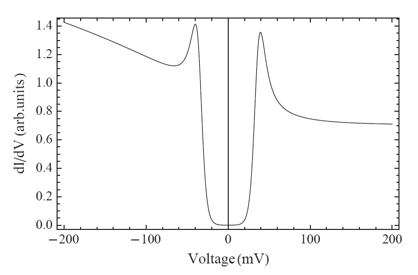
Figure 16: SIN tunneling conductance, exhibiting $U$-shaped feature at low-bias, calculated at $T=40$ K using the simple model with single $s$-wave BCS-like gap $\Delta_{F}$=35 meV and single polaronic gap $\Delta_{p}$=40 meV.

The parameters $G(\varepsilon_{F})$ and $a_{F}(T)$ are adjusted to the experimental data. For the case of single polaronic gap $\Delta_{p}$ and single BCS gap $\Delta_{F}$ the SIN tunneling conductance exhibits a rounded $U$-shaped spectral behavior at low bias (Fig. 16) and such a flat subgap conductance would be expected for homogeneous high-$T_{c}$ cuprates. We argue that the dip-hump feature and asymmetric peaks (with the higher peak in the negative bias voltage) result from the simple superposition of tunneling conductances associated with the BCS DOS and quasi-free state DOS. In the single-gap model, the experimental gap in the tunneling spectra of high-$T_{c}$ cuprates measured as half the energy separating the conductance peaks represents the BCS gap $\Delta_{F}$, while the dip-like feature at energy $|eV|\sim 2\Delta_{F}$, often accompanied by a hump (i.e., almost linearly increasing conductance) at higher energy, is indicative of the presence of polaronic gap $\Delta_{p}$ in their excitation spectrum.

Figure 16 shows clearly that the theoretical tunneling spectra at negative bias just like experimental tunneling conductance curves are characterized by three features: a sharp conductance peak separated from the Fermi level by a BCS-like gap $\Delta_{F}$ and a broad hump at higher energies, $\Delta_{p}$ separated by a well-defined dip at energy $\sim 2\Delta_{F}$. The dip-like feature has particular meaning in the present model, being a consequence of the superposition of the quasi-free state DOS (originating from the polaron dissociation) with the slow decrease of the BCS DOS tail. The polaronic pseudogap in underdoped cuprates is larger than the BCS gap (see Sec. III). As a result, the dip-hump feature will be pronounced in the tunneling spectrum of underdoped cuprates. While the dip feature in the tunneling spectrum of overdoped cuprates becomes weaker due to the weakening of the polaronic effect.

IV.9 2. Multiple-gap model and $V$-shaped tunneling spectra

The physics of quasiparticle tunneling from the cuprate superconductor to the normal metal and vice versa is essentially influenced by the doping-induced inhomogeneities. Therefore, the inhomogeneous high-$T_{c}$ cuprates show very different, asymmetric and more V-shaped spectra with different local tunneling gaps, which might be expected not only within the $d$-wave gap model, but also within the $s$-wave multiple-gap model. One can expect that the electronic inhomogeneity in high-$T_{c}$ cuprates may produce regions with different doping levels and gap amplitudes $(\Delta_{F}(i)$ and $\Delta_{p}(i))$ and a variation in the local DOS. STM and STS experiments on Bi-2212 and other high-$T_{c}$ cuprates confirm this conclusion and indicate that the gap inhomogeneity commonly exists in these high-$T_{c}$ materials regardless of doping level 127 ; 159 ; 160 . Motivated by these experimental observations, we consider the multiple-gap case and the multi-channel tunneling processes (which contribute to the tunneling current) and generalize the above simple model to the case of inhomogeneous cuprate superconductor, where the Fermi energy, BCS gap, polaronic gap and local DOS in various metallic microregions (or stripes) will be different and denoted by $\varepsilon_{Fi}$, $\Delta_{F}(i)$, $\Delta_{p}(i)$, $D_{BCS}(E,\Delta_{F}(i))$ and $D_{f}(E,\Delta_{p}(i))$, respectively $(i=1,2,...)$.

For $V>0$, the tunneling of electrons from the normal metal into these metallic microregions of high-$T_{c}$ cuprate superconductor with different BCS DOS $D_{BCS}(E,\Delta_{F}(i))$ takes place and the contribution of the $i$-th N$\rightarrow$S tunneling channel to the total tunneling conductance is given by Eq. (79). In this case the resulting conductance is

$$\frac{dI_{N\rightarrow S}}{dV}=\sum_{i}G_{i}[A_{1i}(\Delta_{T}(i),a_{V})+$$

$$A_{2i}(\Delta_{T}(i),a_{V})].$$ (82)

For $V<0$, the contributions of parallel conduction channels to the S$\rightarrow$N tunneling current come from various metallic microregions of cuprate superconductors at the dissociation of different polaronic Cooper pairs and large polarons. Therefore, the total current is the sum of tunneling currents flowing from these metallic microregions of cuprate superconductor with different local DOS ($D_{BCS}(E,\Delta_{F}(i))$ and $D_{f}(E,\Delta_{p}(i))$) to the normal metal. The contribution of the $i$-th S$\rightarrow$N tunneling channel into the total tunneling conductance is given by Eq. (IV.8). Then the resulting conductance is

$$\frac{dI_{S\rightarrow N}}{dV}=\sum_{i}G_{i}\{A_{1i}(\Delta_{T}(i),-a_{V})+$$

$$A_{2i}(\Delta_{T}(i),-a_{V})+a_{Fi}(T)[B_{1i}(\Delta_{p}^{*}(i),a_{V})+$$

$$B_{2i}(\Delta_{p}^{*}(i),a_{V})]\}.$$ (83)

In such a multiple-gap model, the tunneling spectra exhibit a more $V$-shaped behavior at low bias, the peak-dip-hump feature at negative bias and the asymmetry of the conductance peaks. The shape of the SIN tunneling spectra between the two conductance peaks tends to be more $V$-shaped in the inhomogeneous multiple-gap regions (with different local gap amplitudes $\Delta_{F}(i)$ and $\Delta_{p}(i)$) due to the superposition of different BCS tunneling conductances, and more rounded $U$-shaped in the homogeneous single gap regions. Indeed, Fang et al. observed such two types of spectra, one nearly $V$-shaped in the average- and large-gap regions and the other showing more rounded $U$-shaped in the small-gap regions of inhomogeneous Bi-2212 160 . With increasing temperature, the dip and peak on the negative bias side gradually disappear 158 , leaving a feature similar to the hump, while the second conductance peak persists on the positive bias side, as observed in tunneling experiments 127 ; 152 .

IV.10 3. Relation to experiments

The experimental tunneling spectra of the well-studied high-$T_{c}$ cuprates Bi-2212 127 ; 160 show the asymmetric and very different V-shaped gaps characterized by the small gaps and sharp well-defined conductance peaks, average gaps and relatively broad conductance peaks, and large gaps and too broad conductance peaks. We now compare our theoretical tunneling spectra calculated using the multiple-gap model with the well-established experimental SIN tunneling data on Bi-2212. The parameters entering into Eqs. (IV.9) and (IV.9) can be varied to fit experimental data. In our analysis we took into account the possible gap inhomogeneity in overdoped, underdoped and strongly underdoped microregions in each sample of Bi-2212. The comparison of the theoretical results with the experimental data on underdoped, slightly underdoped and overdoped Bi-2212 is presented in Fig. 17. We obtained the best fits to the experimental spectra by taking only two or three terms in Eqs. (IV.9) and (IV.9). In this way, we succeeded in fitting almost all of experimental conductance curves by taking two or three (BCS and polaronic) gaps with different gap values. Various V-shaped subgap features, the asymmetric peaks and the dip-hump features, their temperature dependences observed in tunneling spectra of underdoped Bi-2212 (left inset in Fig. 17), slightly underdoped Bi-2212 (right inset in Fig. 17) and overdoped Bi-2212 (main panel in Fig. 17) are adequately reproduced using the multiple-gap model.

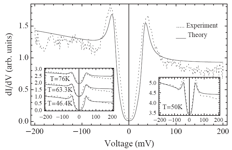
Figure 17: Main panel: SIN tunneling spectrum measured on overdoped Bi-2212 at 43.1 K (dashed line) 161 is fitted by using two-gap model (solid line), with $\Delta_{F}$=31 meV (for $\lambda^{*}_{p}$= 0.5298) and 18 meV (for $\lambda^{*}_{p}$= 0.4154); $\Delta_{p}$= 22 and 15 meV. Left inset: fits of SIN tunneling spectra measured on underdoped Bi-2212 161 by using three-gap model, with $\Delta_{p}$=50, 30 and 25 meV and the set of gap values $\Delta_{F}$=38 meV (for $\lambda^{*}_{p}$= 0.5899), 26 meV (for $\lambda^{*}_{p}$= 0.4866) and 17 meV (for $\lambda^{*}_{p}$= 0.4073) for 46.4 K, $\Delta_{F}$= 37.966 meV, 25.7718 meV and 16.1064 meV; for 63.3 K and $\Delta_{F}$= 37.874 meV, 25.3622 meV and 14.7637 meV for 76 K. Right inset: fit of SIN tunneling spectrum measured on slightly underdoped Bi-2212 at 50 K 162 by using two gap model, with $\Delta_{F}$=36 meV (for $\lambda^{*}_{p}$= 0.5729) and 23 meV (for $\lambda^{*}_{p}$= 0.4694); $\Delta_{p}$= 71 and 37 meV.

The high energy part of the experimental tunneling spectra on the negative bias side show a broad linewidth which grows almost linearly in energy and the peak-dip separation decreases with overdoping. As can be seen in Fig. 17, the agreement of the theory with the well-known experimental results of Renner et al. 161 and Matsuda et al. 162 is fairly good, though the conductance peak heights in some tunneling spectra of Bi-2212 are somewhat underestimated for the overdoped and slightly underdoped samples. Some difference between the calculated and measured conductance peaks can be due to several reasons such as the quality of the sample surface and tip-sample contact 127 , the influence of experimental conditions on tunneling measurements (e.g., the natural surface contamination 163 ), the local variation of the temperature. Tunneling experiments suggest that there exist different types of SIN tunneling spectra that disagree with each other. For example, the opposite asymmetries and doping dependences of the conductance peaks observed in the SIN tunneling experiments on underdoped and overdoped Bi-2212 164 and the dips seen in some STM and STS tunneling measurements on both bias sides (see 156 ; 157 ) have not been found in other SIN tunneling experiments 127 ; 152 ; 159 ; 160 ; 161 ; 162 . Considering the possible uncertainties in experimental measurements, the multiple-gap model leads even in the cases of overdoped Bi-2212 (at 43.1K) 161 and slightly underdoped Bi-2212 (at 50 K) 162 to reasonable agreement between the calculated conductance curves and the well-established tunneling experimental data (Fig. 17).

Thus, the main aspects of the problem of SIN tunneling are successfully modeled. The proposed new simple and generalized multiple-gap models of quasiparticle tunneling across the SIN junction based on two different mechanisms for tunneling of charge carriers at positive and negative biases provides an adequate description of the tunneling spectra of high-$T_{c}$ cuprate superconductors. In particular, these models incorporating effects of the polaronic pseudogap, the combined BCS DOS and quasi-free state DOS at negative bias and the gap inhomogeneity, reproduces well the nearly $U$- and $V$-shaped features, peak-dip-hump structure and asymmetry of the conductance peaks and their evolution with temperature and doping, as seen in the reliable tunneling spectra of Bi-2212 127 ; 159 ; 160 . Interestingly, the peak, dip and hump feature all move to higher binding energy due to the increasing of the BCS-like pseudogap $\Delta_{F}$ and the polaronic pseudogap $\Delta_{p}$ with underdoping. Such a shift of the peak, dip and hump position to higher binding energy with underdoping was actually observed both in tunneling experiments 127 and in ARPES experiments 45

The unusually large reduced-gap values $2\Delta_{F}(0)/k_{B}T_{c}\simeq 7-22$ observed in Bi-2212 127 compared to the BCS value 3.53 give evidence that the BCS-like gap determined by tunneling and ARPES measurements does not close at $T_{c}$ and it is not related to the superconducting order parameter. While the peak suppression on the negative bias side near $T_{c}$ observed in Bi-2212 is due to a spectral superposition of the tunneling conductances associated with the BCS DOS and quasi-free state DOS (originating from the polaron dissociation). The persistence of the conductance peak on the positive bias side well above $T_{c}$ is evidence for the opening of a BCS gap at $T^{*}$.

It is clear that the single-particle tunneling spectroscopy and ARPES provide information about the excitation gaps at the Fermi surface but fail to identify the true superconducting order parameter appearing below $T_{c}$ in non-BCS cuprate superconductors 165 . Therefore, a prolonged discussion of the origin of unconventional superconductivity in the cuprates on the basis of tunneling and ARPES data has nothing to do with the underlying mechanism of high-$T_{c}$ superconductivity; this is because the interpretation of the energy gap observed in tunneling and ARPES experiments both below $T_{c}$ and above $T_{c}$ 43 ; 127 as the evidence for the evolution of a pairing pseudogap from the superconducting order parameter (gap) of high-$T_{c}$ cuprates is misleading speculation.

IV.11 F. Specific heat anomalies of high-$T_{c}$ cuprates in the normal state

The existing experimental facts give evidence that the thermodynamic properties, especially specific heat properties of high-$T_{c}$ cuprate superconductors are very unusual in many respects, both in the superconducting state and in the normal state. In particular, measurements of the specific heat of LSCO and YBCO give clear evidences for the existence of more or less pronounced BCS-like anomalies somewhat above $T_{c}$ or even well above $T_{c}$ 33 ; 59 and a linear term at low temperatures 166 . It seems more likely that the linear term in the low-temperature specific heat of high-$T_{c}$ cuprates is not an intrinsic property of their superconducting state, but due to the presence of some impurity phases 166 . Loram et al. found 167 that the coefficient of the electronic specific heat $\gamma_{e}(T)=C_{e}(T)/T$ in the metallic state of underdoped LSCO and YBCO is no longer constant and shows a broad maximum at some characteristic temperature $T^{*}$ which is much higher than $T_{c}$. In addition to this anomalous feature of $\gamma_{e}(T)$ at $T\leq T^{*}$, the other unexpected and still controversial experimental result is the presence of jump-like anomalies above $T_{c}$ in the specific heat spectrum of high-$T_{c}$ cuprates 166 . The existence of a BCS-like anomaly in electronic specific heat $C_{e}(T)$ of the unconventional cuprate superconductors at $T^{*}>T_{c}$ was assumed by some authors 21 ; 33 ; 168 and this conjecture remains still under discussion 169 . While the other researchers attributed the specific heat jump observed in high-$T_{c}$ cuprates above $T_{c}$ to some kind of phase transition other than the BCS-type phase transition or just simply ignored it. So far, the possible pseudogap effect on $C_{e}(T)$ have not been fully understood. In this subsection we analyze the distinctive specific heat properties of high-$T_{c}$ cuprates in the pseudogap regime and try to provide a natural and quantitative explanation for the specific heat anomalies observed above $T_{c}$ in these materials using the theoretical framework of a pseudogap scenario discussed in Sec. III. One can assume that the BCS-type Cooper pairing of large polarons would occur in the polaronic band below $T^{*}$, while the large polarons localized near the impurities remain impaired. Above $T^{*}$, the contributions to $C_{e}(T)$ come from these two types of charge carriers and the normal-state electronic specific heat is determined from the relation

$$C_{e}(T>T^{*})=(\gamma_{e1}+\gamma_{e2})T,$$ (84)

where $\gamma_{ei}=2\pi^{2}D_{p}(\varepsilon_{Fi})k_{B}^{2}/3=(\pi^{2}/3)k_{B}^{2}g(\varepsilon_{Fi})$ (i=1,2), $g(\varepsilon_{Fi})=3N_{i}/2\varepsilon_{Fi}=3Nf_{i}/2\varepsilon_{Fi}$ is the density of states at the polaronic Fermi level $\varepsilon_{Fi}$ (including both spin orientations), $N_{i}$ is the number of the $i$-th type of large polarons, $N=N_{1}+N_{2}$ is the total number of polaronic carriers in the system , $f_{i}=N_{i}/N$ is the fraction of the $i$-th type of large polaronic carriers. For doped cuprates, the coefficient of the linear term in $C_{e}(T>T^{*})$ is defined as

$$\gamma_{e}=\gamma_{e1}+\gamma_{e2}=\frac{\pi^{2}}{2}k_{B}^{2}xN_{A}\left(\frac{f_{1}}{\varepsilon_{F1}}+\frac{f_{2}}{\varepsilon_{F2}}\right),$$ (85)

where the number of $\rm{CuO_{2}}$ formula unit (or the host lattice atoms) per unit molar volume is equal to the Avogadro number $N_{A}=6.02\times 10^{23}mole^{-1}$, $x=N/N_{A}$ is the dimensionless carrier concentration or doping level, $k_{B}N_{A}=8.314J/moleK$. The important parameters that describe the real experimental situation and the quantitative behavior of $C_{e}(T)$ in doped high-$T_{c}$ cuprate superconductors are $\varepsilon_{Fi}$ and $f_{i}$. Let us estimate the values of $\gamma_{e}$ for LSCO and YBCO. Using the specific values of $\varepsilon_{Fi}$ and $f_{i}$ in the polaronic band ($\varepsilon_{F1}\simeq 0.15$ eV, $f_{1}=0.6$) and impurity band ($\varepsilon_{F2}=0.06$ eV, $f_{2}=0.4$), we obtain $\gamma_{e}\simeq 5.67mJ/moleK^{2}$ at $x=0.1$ for LSCO. The experimental value of $\gamma_{e}$ lies in the range $(4.9-7.3)mJ/moleK^{2}$ 170 . For $\rm{YBa_{2}Cu_{3}O_{7-\delta}}$, the doping level can be determined from the relation 171

$$x(\delta)=\left\{\begin{array}[]{ll}(1-\delta)^{3}&\textrm{for}\>0\leq 1-\delta\leq 0.5,\\ (0.5-\delta)^{3}+0.125&\textrm{for}\>0.5<1-\delta\leq 1\end{array}\right.$$ (88)

from which it follows that $x(\delta=0.115)\simeq 0.182$. By taking $\varepsilon_{F1}=0.20$ eV, $\varepsilon_{F2}=0.1$ eV, $f_{1}=0.6$ and $f_{1}=0.4$ for YBCO, we find $\gamma_{e}\simeq 4.65mJ/moleK^{2}$. This value of $\gamma_{e}$ is well consistent with the experimental data $\gamma_{e}\simeq 4.3-4.9mJ/{moleK^{2}}$ 172

Below $T^{*}$, three contributions to $C_{e}(T)$ come from: (i) the Bogoliubov-like quasiparticles appearing at the dissociation (excitation) of Cooper pairs in the polaronic band, (ii) the unpaired polarons in the impurity band, and (iii) the ideal Bose-gas of incoherent Cooper pairs. The contribution to $C_{e}(T)$ coming from the Bogoliubov-like quasiparticles is determined from the relation.

$$C_{e1}(T<T^{*})=\frac{g(\varepsilon_{F1})}{k_{B}T^{2}}\int\limits_{0}^{\varepsilon_{A}}f(E)(1-f(E))\times$$

$$\times\left[E^{2}(\xi)-\frac{T}{2}\frac{d\Delta_{F}^{2}(T)}{dT}\right]d\xi,$$ (89)

where ${g(\varepsilon_{F1})}={3N_{A}xf_{1}/2\varepsilon_{F1}}$, $f(E)=\left[e^{E/k_{B}T}+1\right]^{-1}$.

The energy of an ideal Bose-gas below the BEC temperature $T_{BEC}$ is given by 173

$$U=0.77n_{c}k_{B}T(T/T_{BEC})^{3/2},$$ (90)

where $n_{c}$ is the number of Bose particles. The specific heat of such a Bose-gas of incoherent Cooper pairs is determined from the relation

$$C_{e3}(T<T^{*})=\frac{dU}{dT}=1.925k_{B}n_{c}\left(T/T_{BEC}\right)^{3/2}.$$ (91)

Then the total electronic specific heat below $T^{*}$ is given by

$$C_{e}(T<T^{*})=C_{e1}(T)+C_{e2}(T)+C_{e3}(T),$$ (92)

where $C_{e2}(T<T^{*})=(\pi^{2}/3)k^{2}_{B}g(\varepsilon_{F2})T$, $g(\varepsilon_{F2})=3N_{A}xf_{2}/2\varepsilon_{F2}$.

The BCS-like gap, $\Delta_{F}(T)$ appearing below $T^{*}$ is determined from Eq. (36). In order to calculate the derivative of $\Delta^{2}_{F}(T)$ with respect to $T$ this BCS-like gap just below $T^{*}$ may be defined as 169

$$\Delta_{F}(T)\simeq 3.06k_{B}T^{*}\sqrt{1-T/T^{*}},$$ (93)

which turns out to be a good approximation only in the narrow temperature range $0.9T^{*}<T\leq T^{*}$. So, if we want a more accurate approximation to find $d\Delta^{2}_{F}(T)/dT$ in a wide temperature range below $T^{*}$, then we can use a more accurate analytical expression (61) for $\Delta_{F}(T)$. As can be seen in Fig. 18, the expression (61) is the best approximation to the BCS-like gap equation not only just below $T^{*}$ but also far below $T^{*}$.

Figure 18: The BCS-like gap $\Delta_{F}$ calculated as a function of the reduced temperature $T/T^{*}$ using the expressions (36) (open circles) at $\lambda^{*}_{p}=0.57$ and $T^{*}=100$K, the expression (61) (solid line 1) at $T^{*}=100$K and the expression (93) (solid line 2) at $T^{*}=100$K.

The number of incoherent Cooper pairs $N_{c}$ and their BEC temperature are determined from the relations

$$n_{c}=\frac{1}{4}g(\varepsilon_{F1})\int\limits_{-\varepsilon_{A}}^{\varepsilon_{A}}\left[1-\frac{\xi}{E}\right]\frac{e^{E/k_{B}T}}{e^{E/k_{B}T}+1}d\xi,$$ (94)

and

$$T_{BEC}=\frac{3.31\hbar^{2}n_{c}^{2/3}}{k_{B}m_{c}},$$ (95)

where $m_{c}=2m_{p}$ is the mass of polaronic Cooper pairs, $\varepsilon_{F1}>\varepsilon_{A}>0.1$ eV, $m_{p}\simeq 2m_{e}$ 89 .

Numerical calculations of $n_{c}$ and $T_{BEC}$ show that just below $T^{*}$ the value of $T_{BEC}$ is very close to $T^{*}$ (i.e., $T_{BEC}\gtrsim T^{*}$), but somewhat below $T^{*}$, $T_{BEC}>>T^{*}$. We emphasize that the calculated results for $C_{e}(T\leq T^{*})$ and $C_{e}(T>T^{*})$ depend sensitively on details of the distribution of polaronic carriers between the polaronic band and the impurity band through the variation of both $\varepsilon_{Fi}$ and $f_{i}$. Actually, the behavior of $C_{e}(T)$ is sensitive to the choice of the parameters $\varepsilon_{Fi}$, $f_{i}$, $x$ and leads us to conclude that self-consistent calculations which take into account changes in the distribution of relevant charge carriers between the polaronic band and the impurity band should be used in comparing with experiment. For doped high-$T_{c}$ cuprates, the observed temperature dependence of $C_{e}$ can be obtained by a more appropriate choice and a careful examining of the relevant fitting parameters. Such a fit is essential for matching the theory with the experiments on $C_{e}(T)$ in various high-$T_{c}$ cuprates. The competition between the pseudogap and impurity effects on $C_{e}(T)$ determines the shape and size of the possible BCS-type jumps of $C_{e}(T)$ above $T_{c}$ in underdoped to optimally doped high-$T_{c}$ cuprates.

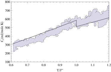
Figure 19: Electronic specific heat of LSCO with doping level $x=0.10$ (solid line) calculated as a function of the reduced temperature $T/T^{*}$ below $T^{*}=98K$ using the fitting parameters $\varepsilon_{F1}\simeq 0.1684$ eV, $\varepsilon_{F2}\simeq 0.0365$ eV, $f_{1}=0.59$, $f_{2}=0.41$ and compared with experimental data for LSCO with doping level $x=0.10$ (dotted line) 33 .

When the BCS-type contribution to $C_{e}(T<T^{*})$ coming from the excited Fermi-components of Cooper pairs and from the bosonic Cooper pairs predominates over the contribution coming from the unpaired carriers in the impurity band, the pronounced BCS-type anomaly of $C_{e}(T)$ is expected at $T^{*}$. However, the situation changes markedly if the impurity contribution dominates the BCS-type contribution and the contribution of bosonic Cooper pairs to $C_{e}(T)$. In this case the jumps of $C_{e}(T)$ above $T_{c}$ will be largely modified (i.e., strongly depressed) by the relatively large impurity contribution to the $C_{e}(T)$ and become less pronounced BCS-type anomalies, as observed in experiments 33 ; 174 . Theoretical results obtained for $C_{e}(T\leq T^{*})$, which are compared with the experimental data on the electronic specific heat reported by Oda’s group for LSCO, are presented in Fig. 19 for the temperature region $0.6T^{*}<T\leq 1.2T^{*}$. Note that the observed behavior of $C_{e}(T)$ closely resembles the calculated results for $T\leq T^{*}$ and $T>T^{*}$, shown in Fig. 19. It follows from the experimental data (see smeared regions between dotted lines in Fig. 19) that the spread of the values of $C_{e}(T)$ are large enough. Nevertheless, there is more or less pronounced BCS-type jump in $C_{e}(T)$ close to $T^{*}$ in LSCO. As seen in Fig. 19, the jump of $C_{e}(T)$ near $T^{*}$ is similar, in both shape and size, to the step-like BCS anomaly, which is observed in high-$T_{c}$ cuprates above $T_{c}$ 33 ; 60 . The specific heat anomaly in the $200-240$ K temperature range, discovered by Fossheim et al. in an YBCO mono-crystal 59 was ascribed to some cause other than that related to the Cooper-pair formation.

However, we argue that this normal-state specific heat anomaly observed also near $220K$ by other authors (for a review, see Ref. 166 ) in YBCO might be a BCS-type anomaly of $C_{e}(T)$ around $T^{*}\simeq 220K$. Dunlap et al. 174 also reported the existence of a phase transition in LSCO at $T^{*}\approx 80K$, which is probably associated with a BCS-type transition at the pseudogap formation temperature. While Loram et al. argued 167 that there is no such a phase transition in the normal state of high-$T_{c}$ cuprates. But they have found that $\gamma_{e}$ is insensitive to $T$ above the characteristic pseudogap temperature $T^{*}$ and decreases rapidly below $T^{*}$ just like in BCS-like theory.

Thus, considering the possible noises or errors in experiments and large enough spread of experimental points (e.g., in Fig. 19), our calculated results for $C_{e}(T)$ are in fair quantitative agreement with the experimental data on $C_{e}(T)$ for high-$T_{c}$ cuprates. In particular, the fitting curve $C_{e}(T)$ in Fig. 19 lies within the experimental noises and is therefore acceptable. Although, at first glance some experimental data on $C_{e}(T)$ do not seem to exhibit significant jump-like anomalies above $T_{c}$ at all, but closer inspection, reveals breaks of the slope of $C_{e}(T)$ or $C_{e}(T)/T$ at various temperatures $T>T_{c}$ in high-temperature cuprates. We therefore may assume that there are BCS-type phase transitions at the breaks of the slope of $C_{e}(T)$ at $T^{*}=T_{break}$ in the cuprates. From the above considerations, it follows that the expected BCS-type jumps of the electronic specific heat of high-$T_{c}$ cuprate superconductors at $T^{*}>T_{c}$ are often buried within the noises and observed as the less pronounced jumps due to the impurity and sample inhomogeneity effects.

IV.12 G. Polaronic isotope effects on the pseudogap formation temperature in high-$T_{c}$ cuprates

The experimental observations of the isotope effects on the pseudogap formation temperature $T^{*}$ in high-$T_{c}$ cuprates 46 ; 175 ; 176 also reflect the fact that the precursor Cooper pairing persists above $T_{c}$. The oxygen and copper isotope effects on $T^{*}$ strongly indicate that the unconventional electron-lattice interactions are involved in the formation of the pseudogap state in these polar materials. The polaronic effect leads to the possibility of observing an unusual isotopic dependence of the Cooper pairing temperature $T^{*}$. Actually, the polaronic nature of charge carriers in high-$T_{c}$ cuprates provides a novel isotope effect due to the dependence of $m_{p}$ on the ionic mass $M$.

The polaronic effects may change significantly the simple BCS picture and lead to the novel isotope effects on $T^{*}$. In the large polaron theory, $m_{p}$, $E_{p}$ and $\varepsilon_{F}$ depend on the Fröhlich-type electron-phonon coupling constant $\alpha_{F}$ which in turn depends on the masses $M(=M_{O}$ or $M_{Cu})$ and $M^{{}^{\prime}}(=M_{Cu}$ or $M_{O})$ of the oxygen O and copper $\rm{Cu}$ atoms in cuprates:

$$\alpha_{F}=\frac{e^{2}}{2\hbar\omega_{0}}\left[\frac{1}{\varepsilon_{\infty}}-\frac{1}{\varepsilon_{0}}\right]\left(\frac{2m\omega_{0}}{\hbar}\right)^{1/2},$$ (96)

where $\omega_{0}\simeq\left(2\kappa\left(\frac{1}{M}+\frac{1}{M^{{}^{\prime}}}\right)\right)^{1/2}$, $\kappa$ is a force constant of the lattice, $m$ is the mass of the undressed carrier in a rigid lattice (i.e. in the absence of the electron-phonon interaction). In the intermediate electron-phonon coupling regime the mass and binding energy of a large polaron are given by 177

$$m_{p}=m(1+\alpha_{F}/6)$$ (97)

and

$$E_{p}=\alpha_{F}\hbar\omega_{0}.$$ (98)

The exponent of the isotope effect on the pseudogap formation temperature $T^{*}$ is defined as

$$\alpha_{T^{*}}=-\frac{d\ln{T^{*}}}{d\ln{M}}.$$ (99)

Using Eqs. (45), (97) and (98), we find that Eqs. (47) (at $\lambda_{p}\lesssim 0.5$ and $C^{*}=1.134$) and (99), become

$$k_{B}T^{*}=1.134A^{*}\mu^{-1/4}\left(1+a^{*}\mu^{-1/4}\right)\exp\left[-1/\lambda_{p}^{*}(\mu)\right],$$

and

$$\alpha_{T^{*}} = \frac{1}{4(1+M/M^{{}^{\prime}})}\left\{1+\frac{a^{*}\mu^{-1/4}}{1+a^{*}\mu^{-1/4}}-\frac{1}{(\lambda_{l}^{*}(\mu))^{2}}\right.$$ (101)

$$\left.\times\left(\lambda_{ph}b^{*}\mu^{1/4}-\frac{\lambda_{c}b^{*}\mu^{1/4}}{U_{c}(\mu)}+\frac{\lambda_{c}^{2}(1+b^{*}\mu^{1/4})}{U^{2}_{c}(\mu)}\right.\right.$$

$$\left.\left.\times\left[b^{*}\mu^{1/4}\ln{B^{*}(\mu)}\right.\right.\right.$$

$$\left.\left.\left.+(1+b^{*}\mu^{1/4})\left(1+\frac{a^{*}\mu^{-1/4}}{1+a^{*}\mu^{-1/4}}\right)\right]\right)\right\},$$

where $\lambda_{p}^{*}(\mu)=\lambda_{ph}(1+b^{*}\mu^{1/4})-\lambda_{c}(1+b^{*}\mu^{1/4})/U_{c}(\mu)$, $U_{c}(\mu)=1+\lambda_{c}(1+b^{*}\mu^{1/4})\ln{B^{*}(\mu)}$, $\lambda_{ph}=\left[2m/\hbar^{2}(3\pi^{2}n)^{2/3}\right]V_{ph}$, $\lambda_{c}=\left[2m/\hbar^{2}(3\pi^{2}n)^{2/3}\right]V_{c}$, $B^{*}(\mu)=\varepsilon_{F}/A^{*}\mu^{-1/4}\left(1+a^{*}\mu^{-1/4}\right)$, $A^{*}=\frac{e^{2}}{\tilde{\varepsilon}}\sqrt{\frac{m}{2\hbar}}(2k)^{1/4}$, $a^{*}=\hbar\tilde{\varepsilon}\sqrt{\frac{2\hbar}{m}}(2\kappa)^{1/4}/e^{2}$, $b^{*}=1/6a^{*}$, $\mu=MM^{{}^{\prime}}/(M+M^{{}^{\prime}})$ is the reduced mass of ions.

Some experiments showed that the oxygen and copper isotope effects on the pseudogap temperature $T^{*}$ in $\rm{Y}$- and $\rm{La}$- based cuprates are absent or very small 178 ; 179 ; 180 and sizable 179 ; 181 . While other experiments revealed a huge oxygen isotope effect on the charge ordering (CO) temperature $T_{CO}$ in LSCO 182 (where the pseudogap formation temperature $T^{*}$ is identified with $T_{CO}$) and the large negative oxygen and copper isotope effects on $T^{*}$ in $\rm{Ho}$-based cuprates 179 ; 183 . The oxygen isotope effect on $T^{*}$ observed in high-$T_{c}$ cuprates is turned out to be unusual and, most interestingly, sign reversed, while the copper isotope effect in the $\rm{HoBa_{2}Cu_{4}O_{8}}$ system is much larger than the oxygen isotope effect. These and other observations 176 suggest that the unconventional electron-phonon interactions and polaronic effects play an important role in high-$T_{c}$ cuprates and could be the origin of the unusual isotope effect. Below, we will show that Eqs. (IV.12) and (101) predict the existence of such a novel isotope effect on $T^{*}$ observed in various high-$T_{c}$ cuprates.

Note that the expression for $\alpha_{T^{*}}$, Eq.(101) contains not only the electron-phonon coupling constant $\lambda_{ph}$ and Coulomb parameter $\lambda_{c}$, but also the effective BCS-like coupling constant $\lambda^{*}_{p}(\mu)$, carrier concentration $n$ and parameters ($\tilde{\varepsilon}$, $\kappa$, $M$, $M^{\prime}$ and $\mu$) of the cuprates. With Eqs. (IV.12) and (101) one can explain the specific features of both the oxygen isotope effect (evaluating Eq. (101) at $M=M_{O}$ and $M^{\prime}=M_{Cu}$) and the copper isotope effect (evaluating Eq. (101) at $M=M_{Cu}$ and $M^{\prime}=M_{O}$) in cuprates. These equations allow us to calculate the pseudogap formation temperatures $T^{*}$ and the exponents $\alpha^{O}_{T^{*}}$ and $\alpha^{Cu}_{T^{*}}$ of the oxygen and copper isotope effects on $T^{*}$. For the cuprates, we will use the experimental values of dielectric constants $\varepsilon_{\infty}=3-5$ and $\varepsilon_{0}=22-50$ presented in Refs. 76 ; 89 to determine the possible values of $\tilde{\varepsilon}$. By using the well-established experimental values of $\varepsilon_{\infty}=3-5$ and $\varepsilon_{0}=22-30$ 76 ; 89 , we find $\tilde{\varepsilon}=3.33-6.47$. After that, inserting the values of $\tilde{\varepsilon}$ into Eqs. (IV.12) and (101), we calculate the pseudogap formation temperatures $T^{*}$ and the oxygen and copper isotope exponents $\alpha^{O}_{T^{*}}$ and $\alpha^{Cu}_{T^{*}}$, which are then compared to their measured values in various high-$T_{c}$ cuprates. In our numerical calculations, we also take $m\simeq m_{e}$ 89 and $\hbar\omega_{0}=0.04-0.07$ eV 81 ; 89 . Then we obtain $\alpha_{F}=2.15-5.54$ (which correspond to the intermediate electron-phonon coupling regime). The $\ln{B^{*}(\mu)}$ entering into the expressions for $T^{*}$ and $\alpha_{T^{*}}$ will be small, so that the Coulomb pseudopotential $\tilde{V}_{c}$ is of the order of bare Coulomb potential $V_{c}$. Although the expressions for the pseudogap formation temperature $T^{*}$ and the isotope exponent $\alpha_{T^{*}}$ depend on various parameters, part of these parameters ($m$, $M$, $M^{\prime}$, $\mu$, $\tilde{\varepsilon}$ and $\kappa$) have been previously determined experimentally and are not entirely free (fitting) parameters for the considered high-$T_{c}$ cuprates (e.g., $\kappa$ is fixed at the value estimated for the oxygen and copper unsubstituted compound using the value of $\hbar\omega_{0}=0.05$ eV). Therefore, only some parameters $\tilde{\varepsilon}$, $n$, $V_{ph}$ and $V_{c}$ should have different values in different samples of high-$T_{c}$ cuprates. These parameters can be examined for specific input parameters $T^{*}$ and $\alpha_{T^{*}}$. For the given ionic masses $M$ and $M^{\prime}$, Eqs. (IV.12) and (101) have to be solved simultaneously and self-consistently to determine $T^{*}$ and the isotope effect on $T^{*}$. Then, replacing in these equations the oxygen ion mass ${}^{16}\rm{O}$ by its isotope ${}^{18}\rm{O}$ mass and keeping all other parameters identical to the case ${}^{16}\rm{O}$, $T^{*}$ is calculated again and the isotope shift $\Delta T^{*}=T^{*}(^{18}O)-T^{*}(^{16}O)$ is calculated for ${}^{16}\rm{O}\longrightarrow^{18}\rm{O}$ substitution. The isotope shift $\Delta T^{*}=T^{*}(^{65}Cu)-T^{*}(^{63}Cu)$ is calculated in the same manner for ${}^{63}\rm{Cu}\longrightarrow^{65}\rm{Cu}$ substitution. The results of numerical calculations of $T^{*}$ and $\alpha_{T^{*}}$ at different values of $\tilde{\varepsilon}$, $n$, $\lambda_{ph}$ and $\lambda_{c}$ are shown in Figs. 20-23.

Our results provide a consistent picture of the existence of pseudogap crossover temperatures $T^{*}$ above $T_{c}$ and various isotope effects on $T^{*}$ in high-$T_{c}$ cuprates. They explain why the small positive or even sign reversed (see Fig. 20) and very large negative (see Figs. 21 and 22) oxygen isotope effects and the large negative and negligible (Fig. 23) copper isotope effects on $T^{*}$ are observed in various experiments. The values of $\lambda_{p}^{*}$ varies from 0.3 to 0.5 and $T^{*}$ increases with decreasing $n$. The existing experimental data on $T^{*}$ and $\alpha_{T^{*}}$ for $\rm{YBa_{2}Cu_{4}O_{8}}$, $\rm{HoBa_{2}Cu_{4}O_{8}}$ and $\rm{La_{1.96-x}Sr_{x}Ho_{0.04}CuO_{4}}$ could be fitted with an excellent agreement using Eqs. (IV.12) and (101), and adjusting the parameters $\tilde{\varepsilon}$, $n$, $\lambda_{ph}$ and $\lambda_{c}$ for each cuprate superconductor. One can assume that in $\rm{YBa_{2}Cu_{4}O_{8}}$ and $\rm{HoBa_{2}Cu_{4}O_{8}}$ the optimally doped level corresponds to the value $n\geq 0.9\times 10^{21}\rm{cm^{-3}}$. Provided $n=0.925\times 10^{21}\rm{cm^{-3}}$, $\tilde{\varepsilon}=4.715-4.905$, $V_{ph}\simeq 0.10$ eV and $V_{c}\simeq 0.025$ eV, one can see that $T^{*}=150-161K$ and $\alpha^{O}_{T^{*}}$ is very small (i.e., $\alpha^{O}_{T^{*}}=(0.0031-0.0069)<0.01$), which are consistent with the experimental data of Refs. 178 ; 180 for $\rm{YBa_{2}Cu_{4}O_{8}}$. Further, using other sets of parameters $n=0.93\times 10^{21}\rm{cm^{-3}}$, $\tilde{\varepsilon}=6.087-6.389$, $V_{ph}\simeq 0.1188$ eV and $V_{c}=0.0313$ eV, we obtain $T^{*}\approx 150K$ and $\alpha^{O}_{T^{*}}\simeq 0.053-0.059$ (Fig. 20), which are in fair agreement with the measured values: $T^{*}=150K$ and $\alpha^{O}_{T^{*}}=0.052-0.061$ for $\rm{YBa_{2}Cu_{4}O_{8}}$ (with $T_{c}=81K$) 181 . Figure 20 illustrates the predicted behaviors of $\alpha^{O}_{T^{*}}$ as a function of $\tilde{\varepsilon}$ and we see that $\alpha^{O}_{T^{*}}$ is small and may become negative with decreasing $\tilde{\varepsilon}$ and the difference $V_{ph}-V_{c}$. Relatively strong electron-phonon and Coulomb interactions change the picture significantly and cause $\alpha^{O}_{T^{*}}$ to decrease rapidly with decreasing $\tilde{\varepsilon}$ (Fig. 21) or increasing $n$ (Fig. 22). In this case the value of $\alpha^{O}_{T^{*}}$ is negative and becomes very large negative with decreasing $\tilde{\varepsilon}$. The pictures shown in Figs. 21 and 22 are likely realized in some cuprates (which exhibit a large negative isotope exponent $\alpha^{O}_{T^{*}}$) and explain another important puzzle of the cuprates 183 : the huge oxygen isotope effect on $T^{*}$ observed in $\rm{HoBa_{2}Cu_{4}O_{8}}$, whose characteristic pseudogap temperature $T^{*}$ increases significantly upon replacing $\rm{{}^{16}O}$ by $\rm{{}^{18}O}$.

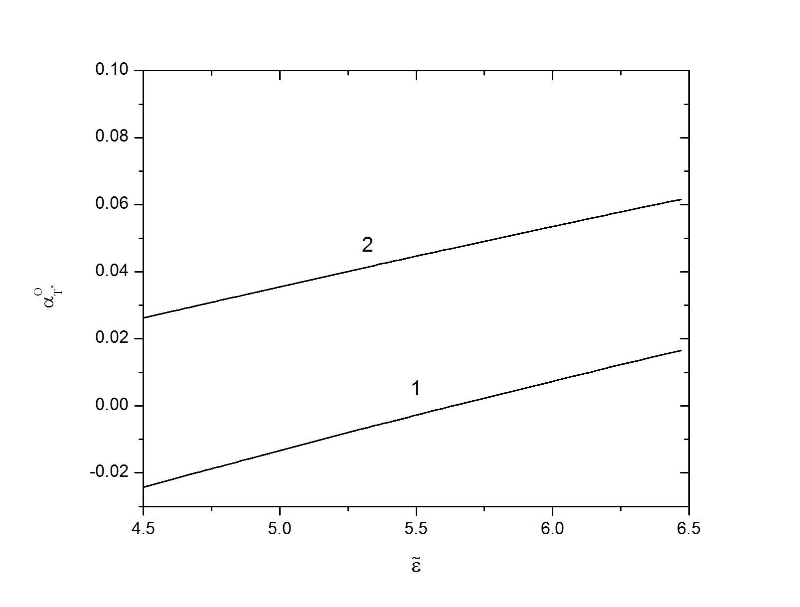
Figure 20: Variation of $\alpha^{O}_{T^{*}}$ as a function of $\tilde{\varepsilon}$ for two sets of parameters: (1) $V_{ph}=0.1175$ eV, $V_{c}=0.0313$ eV, $n=0.89\times 10^{21}\rm{cm^{-3}}$ and (2) $V_{ph}=0.1188$ eV, $V_{c}=0.0313$ eV, $n=0.93\times 10^{21}\rm{cm^{-3}}$.

Figure 21: The dependence of $\alpha^{O}_{T^{*}}$ on $\tilde{\varepsilon}$ for $V_{ph}=0.296$ eV, $V_{c}=0.208$ eV and $n=0.9\times 10^{21}\rm{cm^{-3}}$.

Figure 22: The doping dependence of $\alpha^{O}_{T^{*}}$ (main panel) and $\lambda_{p}^{*}(\mu)$ (inset) for $V_{ph}=0.296$ eV, $V_{c}=0.208$ eV and $\tilde{\varepsilon}=4.109$.

Figure 23: The dependence of $\alpha^{Cu}_{T^{*}}$ on $\tilde{\varepsilon}$ for $V_{ph}=0.616$ eV, $V_{c}=0.316$ eV and $n=0.9\times 10^{21}\rm{cm^{-3}}$.

Indeed, with fitting parameters, $n=0.9\times 10^{21}\rm{cm^{-3}}$, $\tilde{\varepsilon}\simeq 4.109$, $V_{ph}=0.296$ eV and $V_{c}=0.208$ eV, one can explain the observed experimental data of Ref. 183 . In this case, we obtain $T^{*}(^{16}O)\simeq 170K$, $T^{*}(^{18}O)\simeq 220K$, $\Delta T_{O}^{*}=T^{*}(^{18}O)-T^{*}(^{16}O)\simeq 50K$ and $\alpha^{O}_{T^{*}}\simeq-2.53$, which are in remarkably good agreement with the experimental data $T^{*}(^{16}O)\simeq 170K$, $T^{*}(^{18}O)\simeq 220K$, $\Delta T_{O}^{*}\simeq 50K$ and $\alpha^{O}_{T^{*}}\simeq-2.2\pm 0.6$ 183 . We have also performed similar calculations for the copper isotope effect on $T^{*}$ in slightly underdoped $\rm{HoBa_{2}Cu_{4}O_{8}}$ and for the oxygen and copper isotope effects on $T^{*}$ in optimally doped $\rm{La_{1.81}Ho_{0.04}Sr_{0.15}CuO_{4}}$. Figure 23 shows the predicted behaviors of $\alpha_{T^{*}}^{Cu}$ as a function of $\tilde{\varepsilon}$.

By taking $n=0.9\times 10^{21}\rm{cm^{-3}}$, $\tilde{\varepsilon}=3.334$, $V_{ph}=0.616$ eV, $V_{c}=0.316$ eV for $\rm{HoBa_{2}Cu_{4}O_{8}}$, we find $T^{*}(^{63}Cu)\simeq 160K$, $T^{*}(^{65}Cu)\simeq 184.6K$, $\Delta T_{Cu}^{*}=T^{*}(^{65}Cu)-T^{*}(^{63}Cu)\approx 25K$ and $\alpha_{T^{*}}^{Cu}\simeq-4.86$ in accordance with experimental findings $T^{*}(^{63}Cu)\approx 160K$, $T^{*}(^{65}Cu)\approx 185K$ and $\alpha_{T^{*}}^{Cu}\simeq-4.9$ 184 . In the orthorhombic $\rm{La_{2-x}Sr_{x}CuO_{4}}$ the optimally doped level ($x\simeq 0.15$) corresponds to the value $n=0.8\times 10^{21}\rm{cm^{-3}}$. By taking $\tilde{\varepsilon}=4$, $V_{ph}=0.157$ eV and $V_{c}=0.104$ eV for $\rm{La_{1.81}Ho_{0.04}Sr_{0.15}CuO_{4}}$, we obtained $T^{*}(^{16}O)=T^{*}(^{63}Cu)\simeq 60K$, $T^{*}(^{18}O)\simeq 70K$, $\Delta T^{*}_{O}\simeq 10K$, $T^{*}(^{65}{Cu})\simeq 60.53K$; $\Delta T_{Cu}^{*}\simeq 0.53K$, which agree fairly well with the experimental data of Ref. 179 . Further, using other fitting parameters $n=0.67\times 10^{21}\rm{cm^{-3}}$, $\tilde{\varepsilon}=4.08$, $V_{ph}=0.178$ eV, $V_{c}=0.124$ eV and $n=1.1\times 10^{21}\rm{cm^{-3}}$, $\tilde{\varepsilon}=3$, $V_{ph}=0.124$ eV, $V_{c}=0.069$ eV for moderately underdoped and overdoped systems $\rm{La_{1.96-x}Sr_{x}Ho_{0.04}CuO_{4}}$ (with $x=0.11$ and $x=0.20$), we found $T^{*}(^{16}O)\simeq 80K$, $T^{*}(^{18}O)\simeq 100K$, $\Delta T_{O}^{*}\simeq 20K$ and $T^{*}(^{16}O)\simeq 50K$, $T^{*}(^{18}O)\simeq 54.61K$, $\Delta T_{O}^{*}\simeq 4.61K$ for these $\rm{La}$-based compounds with $x=0.11$ and $x=0.20$, respectively. These results are in good quantitative agreement with the experimental results reported in Ref. 185 for $\rm{La_{1.96-x}Sr_{x}Ho_{0.04}CuO_{4}}$, in which upon oxygen substitution (¹⁸O vs ¹⁶O), $T^{*}$ is shifted upwards by 20 and 5 K for $x=0.11$ and $x=0.20$, respectively.

Thus, our results for $T^{*}$, isotope shifts $\Delta T^{*}$ and exponents ($\alpha_{T^{*}}^{O}$ and $\alpha_{T*}^{Cu}$) in different classes of high-$T_{c}$ cuprates are in good agreement with the existing well-established experimental data and explain the controversy between various experiments 178 ; 180 ; 181 on isotope effects for $T^{*}$ in the cuprates.

V v. Pseudogap phenomena in other unconventional superconductors and superfluids

When the strength of the attractive interaction between fermionic quasiparticles becomes sufficiently strong, the Cooper-like pairing of such quasiparticles can occur at a higher temperature $T^{*}$ than the $T_{c}$ not only in high-$T_{c}$ cuprates but also in other unconventional superconductors and superfluids. Therefore, the idea of a normal state gap in high-$T_{c}$ cuprates might be extended in other exotic systems. In particular, the normal state of organic and heavy-fermion superconductors exhibits a pseudogap behavior above $T_{c}$ and is different from the normal state of conventional BCS superconductors 24 ; 186 . Below $T_{c}$, the behaviors of these superconductors and superfluid ³He are also similar to that of high-$T_{c}$ cuprates. Actually, the BCS-like energy gap in unconventional superconductors and superfluid ³He differs from the superconducting/superfluid order parameter and persists above $T_{c}$.

V.1 A. Pseudogap state in organic superconductors

One can assume that the ground state of charge carriers in organic materials just like in high-$T_{c}$ cuprates is a self-trapped state (polaronic state) with appreciable lattice distortion when the carrier-phonon interaction is strong enough 187 ; 188 . The carrier self-trapping leads to a narrowing of the conduction band and the Cooper-like pairing of polaronic carriers may be considered in the momentum space as in BCS-like theory presented in section III. In organic superconductors the Cooper-like pairing of polaronic carriers and the opening of a pseudogap on the Fermi surface may also occur at a mean-field temperature $T^{*}>T_{c}$. To calculate the pseudogap formation temperature $T^{*}$ in these systems, we use the generalized BCS formalism and the BCS-like gap equation Eq. (36).

The BCS-like gap $\Delta_{F}$ goes to zero continuously as $T$ approaches $T^{*}$ from below and the characteristic pseudogap formation temperature is determined from the equation

$$\frac{1}{\lambda_{p}^{*}}=\int_{0}^{E_{p}+\hbar\omega_{0}}\frac{d\xi}{\xi}tanh(\frac{\xi}{2k_{B}T^{*}}).$$ (102)

At $\lambda_{p}^{*}\lesssim 0.5$ and $E_{p}+\hbar\omega_{0}>6k_{B}T^{*}$ this equation gives (see Table II)

$$k_{B}T^{*}=1.134(E_{p}+\hbar\omega_{0})\exp{(-1/\lambda_{p}^{*})}.$$ (103)

If the Fermi energy $\varepsilon_{F}$ is smaller than $E_{p}+\hbar\omega_{0}$, the cutoff energy $\varepsilon_{A}=E_{p}+\hbar\omega_{0}$ in Eq. (36) for the attractive electron-phonon interaction is replaced by $\varepsilon_{F}$.

Organic superconductors (BEDF-TTF salts) may have high phonon energy up to 0.018 eV 189 . For organic materials, the value of the polaron binding energy $E_{p}$ varies from 0.03 to 0.06 eV 190 , while the value of $\varepsilon_{F}$ varies from 0.07 to 0.10 eV 191 ; 192 . The values of $m_{p}$ are about 3.5-5.0$m_{e}$ 191 ; 192 . At $E_{p}=0.05$ eV, $\hbar\omega_{0}\simeq 0.018$ eV and $\lambda^{*}_{p}=0.38$, we find from Eq. (103) that in organic superconductors the BCS-like pairing pseudogap opens well above $T_{c}$, namely, at $T^{*}\simeq 64K>>T_{c}\simeq 10.4$K (for $\rm{\emph{k}-(BEDT-TTF)Cu[N(CN)_{2}]Br}$ system superconductors 186 ). If we use the values of the parameters $E_{p}=0.038$ eV, $\lambda_{p}^{*}=0.335-0.338$ and $E_{p}=0.04$ eV, $\lambda_{p}^{*}=0.356-0.367$, we obtain $T^{*}\simeq 37-38$ and $T^{*}\simeq 46-50K$, which are in good agreement with the values of $T^{*}=37-38K$ and $T^{*}=46-50K$ observed in organic superconductors $\rm{\emph{k}-(ET)_{2}Cu[N(CN)_{2}]Br}$ and $\rm{\emph{k}-(ET)_{2}Cu[N(NCS)_{2}]}$, respectively 24 . Further, the pseudogap behavior is also observed in $\rm{\emph{k}-(BEDT-TTF)_{2}Cu(NCS)_{2}}$ where the magnitude of the pseudogap is larger than 0.02 eV 186 . In $\rm{\emph{k}-(BEDT-TTF)_{2}Cu(NCS)_{2}}$ ($T_{c}\simeq 10.4$K) the pseudogap disappears at about 45K 186 . By taking $E_{p}=0.04$ eV and $\hbar\omega_{0}\simeq 0.018$ eV for this system, we find $T^{*}\simeq 50$ K at $\lambda_{p}^{*}=0.354$ in accordance with the above experimental results 186 .

V.2 B. Possible Pseudogap States in Heavy-Fermion Systems and Liquid ³He

Experimental data show 17 ; 18 ; 193 ; 194 ; 195 that the heavy-fermion superconductors $\rm{UPd_{2}Al_{3}}$, $\rm{YbAl_{3}}$ and $\rm{CeCoIn_{5}}$, which have many similarities to the high-$T_{c}$ cuprates, also have a pseudogap state above $T_{c}$. The common feature of these compounds is that they contain $f$ electrons having localized orbitals and characterized by the narrow $f$ electron bands, so that the effective masses of charge carriers are very large $m^{*}\simeq 50-200m_{e}$ 18 . The $f$ electrons become partly itinerant when a nearly localized $f$-band is formed and they become completely delocalized due to their strong hybridization with the conduction electrons 18 . The strong interaction of the conduction electrons with nearly localized $f$ electrons leads to an enhanced density of states at the Fermi level. The exchange interactions take place between the magnetic moments of $f$ electrons and the spins of the conduction ($c$) electrons, to cause a new bound (paired) state of charge carriers in heavy-fermion compounds. It is interesting that the properties of heavy-fermion superconductors are similar to those of liquid ³He. Magnetic interactions are surely the most important part of the pairing interaction both in heavy-fermion systems and in liquid ³He. These interactions are likely to produce Cooper pairs above $T_{c}$ in spin-triplet states with an odd orbital angular momentum $l$ and might be relevant for describing the possible pseudogap states in heavy-fermion systems. Magnetic couplings are also thought to arise in liquid ³He and play an important role in the formation of the triplet p-wave pairing states below a superfluid transition temperature $T_{c}$ 196 ; 197 ; 198 . Although the role of unconventional Cooper pairing both in the formation of the superfluid state or in the formation of the pseudogap-like state in ³He is not established, it is likely to be a central importance, as is certainly the case for heavy-fermion systems and possibly also for high-$T_{c}$ cuprates. The theory developed to explain the pseudogap behavior of high-$T_{c}$ cuprates may be also applicable to heavy-fermion superconductors which exhibit a similar behavior in many regards 17 ; 29 . In particular, there are signatures of quasiparticle confinement in the normal state of the heavy-fermion superconductor $\rm{CeCoIn_{5}}$ 195 . The electronic structure of heavy-fermion systems can be described by the nearly localized narrow $f$ band that cause the heavy-fermion behavior and the itinerant $f-c$ hybridized band 199 which is a relatively broad to support superconductivity. In the presence of strong hybridization of the $f$ electrons with electrons on neighboring non-$f$-electron atoms, a competition can exist between localized $f$ electrons (which support magnetism) and itinerant $f-c$ hybridized bands in which the charge carriers having relatively smaller effective masses $m^{*}\simeq 15-30m_{e}$ 18 ; 29 ; 193 ; 194 take part in unconventional Cooper pairing. The Cooper pairs in heavy-fermion superconductors are assumed to be in a spin triplet state with the spin $S=1$ and orbital angular momentum $l=1$, just like the Cooper pairs in liquid ³He. Two possible forms of spin-triplet p-wave pairing in ³He have been studied by Anderson and Model 200 , and Balian and Werthamer 201 . Anderson and Morel considered an equal spin pairing (EPS) ground state (later named the Anderson-Brinkman-Morel (ABM) state) with parallel spins ($S_{z}=\pm 1$) and predicted an anisotropic energy gap that has nodes (i.e., zero-points) on the Fermi surface. Whereas Balian and Werthamer studied the non-ESP ground state containing all three spin substates, $S_{z}=0,\pm 1$ and showed that such a p-wave pairing state (later called the Balian-Werthamer (BW) state) would have an isotropic energy gap (just like $s$-wave BCS gap) and be energetically favorable. Many authors claim that the A and B phases of superfluid ³He are described by the ABM and BW states, respectively. However, the Anderson-Morel and Balian-Werthamer models could not account for the existence of the first-order transition between A and B phases of superfluid ³He. These models predict only the second-order BCS transition at a mean-field pairing temperature $T_{MF}=T^{*}$ which might be different from the superfluid transition temperature $T_{c}$. We believe that the superfluid phase transition in ³He is more similar to the $\lambda$ - transition (see, e.g., Fig. 1.9a presented in Ref. 198 ) than to the step-like BCS one; and the nature of the superfluid phases of ³He is still not understood. It seems likely that the ABM and BM states are possible precursor pairing (or pseudogap-like) states and these states may exist both below $T_{c}$ and above $T_{c}$.

The mean-field pairing temperature $T^{*}$ for ³He and heavy-fermion superconductors is determined from the BCS-like gap equation Eq. (31) (where $V_{p}(\vec{k},\vec{k}^{\prime})$ is replaced by the pair interaction potential $V(\vec{k},\vec{k}^{\prime})$ between the relevant fermionic quasiparticles). In this equation, the expansion of the effective pair interaction function $V(\vec{k},\vec{k}^{\prime})$ in terms of Legendre polynomials $P_{l}(\hat{\vec{k}},\hat{\vec{k}^{\prime}})$ with different $l$ contains the radial part of the p-wave attractive interaction potential $V_{l}(\vec{k},\vec{k})$ which is responsible for the highest mean-field pairing temperature. In the case of the spin-triplet ($S=1$) Cooper pairing, the pair interaction potential can be written as 197

$$V(\vec{k},\vec{k}^{\prime})=\sum\limits_{l=0}^{\infty}(2l+1)V_{l}(\vec{k},\vec{k}^{\prime})P_{l}(\hat{\vec{k}},\hat{\vec{k}^{\prime}}),$$ (104)

where $\hat{\vec{k}}=\vec{k}/k_{F}$, $k_{F}$ is the Fermi wave vector.

Further, the interaction potential $V_{l}(\vec{k},\vec{k}^{\prime})$ is assumed to be constant within a thin layer near the Fermi surface and zero elsewhere:

$$V_{l}(\vec{k},\vec{k}^{\prime})=\left\{\begin{array}[]{ll}-V_{l},&\textrm{for}\>|\xi(k)|,\>|\xi(k^{\prime})|\leq\varepsilon_{A},\\ 0&\>\textrm{otherwise}\end{array}\right.$$ (107)

Substituting Eq. (107) into Eq. (31) and using the angular average over $\hat{\vec{k}}$ 30 , the BCS-like gap equation may be written as

$$1=V_{l}\sum\limits_{\vec{k}^{\prime}}\frac{1}{2E(\vec{k}^{\prime})}\tanh{\frac{E(\vec{k}^{\prime})}{2k_{B}T}},$$ (108)

where $E(\vec{k})=\sqrt{\xi^{2}(k)+\Delta^{2}_{F}(\vec{k})}$. The summation in Eq. (108) over momenta can be replaced by an integral over energies $\varepsilon$ within the thin energy layer near the Fermi surface by introducing the DOS $D(\varepsilon_{F})$. Then the gap equation Eq. (108) reduces to

$$1=V_{l}D(\varepsilon_{F})\int\limits_{0}^{\varepsilon_{A}}\frac{\tanh{(E/2k_{B}T)}}{E}d\xi.$$ (109)

At a mean-field pairing temperature $T^{*}$, $\Delta_{F}(T^{*})=0$, so that for $\varepsilon_{A}>6k_{B}T^{*}$, Eq. (109) yields a relation between the temperature $T^{*}$, the cutoff energy $\varepsilon_{A}$ and the pair interaction constant $V_{l}$:

$$k_{B}T^{*}=1.134\varepsilon_{A}\exp{(-1/\lambda_{l}^{*})},$$ (110)

where $\lambda_{l}^{*}=V_{l}D(\varepsilon_{F})$ is the BCS-like coupling constant.

The Fermi temperature $T_{F}$ in liquid ³He is of the order 1K and the interaction between ³He atoms should be strong enough in order to expect the BCS-like pairing correlation effect well above $T_{c}$. By taking $\varepsilon_{A}\simeq 0.5k_{B}T_{F}$ and $\lambda_{l}^{*}=0.554$, we find $T^{*}\simeq 93$mK. Experimental results show 202 that the heat capacity of liquid ³He exhibits an anomaly near 100 mK and increases linearly with temperature between 100 and 500 mK. It follows that the formation of pseudogap-like state in ³He is expected below 100 mK.

One can assume that the energy of the exchange interaction in heavy-fermion systems just like in undoped cuprates 89 is of the order of $J\gtrsim 0.1$ eV, and the Fermi energy $\varepsilon_{F}$ of these systems will be considerably smaller than $J$. Therefore, the cutoff energy $\varepsilon_{A}$ in Eq. (110) can be replaced by $\varepsilon_{F}$. If the carrier concentration $n_{f}$ in the f-c hybridized band is about $2*10^{21}\rm{cm^{-3}}$, we obtain $\varepsilon_{F}=\hbar^{2}(3\pi^{2}n_{f})^{2/3}/2m^{*}\simeq 0.019-0.039$ eV. In order to determine the pseudogap formation temperatures in heavy-fermion superconductors $\rm{UPd_{2}Al_{3}}$ and $\rm{YbAl_{3}}$, we can take $\varepsilon_{A}=\varepsilon_{F}\simeq 0.04$ eV. Then we obtain the following values of $T^{*}\simeq 40$ K and 50 K at $\lambda_{l}^{*}\simeq 0.425$ and 0.388 respectively. These values of $T^{*}$ are consistent with the pseudogap formation temperatures $T\simeq 40$ K and 50 K observed in heavy-fermion superconductors $\rm{UPd_{2}Al_{3}}$ 18 and $\rm{YbAl_{3}}$ 193 . We now evaluate the pseudogap formation temperature in $\rm{CeCoIn_{5}}$. By taking $\varepsilon_{F}\simeq 0.02$ eV and $\lambda_{l}^{*}\simeq 0.256$ in Eq. (110), we find $T^{*}\simeq 5.3$ K in accordance with the experimental results 194 .

VI VI. Bozonization of Cooper pairs in unconventional superconductors and superfluids

There are key differences between strongly overlapping (weakly-bound) and non-overlapping (tightly-bound) Cooper pairs in superconductors and superfluids. When Cooper pairs begin to overlap strongly, they lose their composite nature under the exchange of their fermionic components, which move away from one Cooper pair to another. These Cooper pairs behave like fermions. In contrast, non-overlapping Cooper pairs behave like bosons. So, the superconductivity (superfluidity) of bosonic Cooper pairs are fundamentally different from the conventional superconductivity (superfluidity) of fermionic Cooper pairs described by the BCS-like ($s$-, $p$- or $d$- wave) pairing theory. A distinctive feature of unconventional superconductors and superfluids is that they might be in the bosonic limit of Cooper pairs. Therefore, in this section we study the possibility of the existence of bosonic Cooper pairs in unconventional superconductors and superfluids. As the binding between fermions increases, Fermi gas of large overlapping Cooper pairs evolves into Bose gas of small non-overlapping Cooper pairs, as pointed out by Leggett 69 . This is the most interesting crossover regime, since a Fermi system passes from a BCS-like Fermi-liquid limit to a normal Bose gas limit with decreasing $\varepsilon_{F}$. Thus, it is a challenging problem to find the possible criteria for bosonization of Cooper pairs in such Fermi systems depending on the threshold values of system parameters. In the following, we formulate such criteria for bosonization of Cooper pairs depending on two and three basic parameters of unconventional superconductors and superfluids.

VI.1 A. The criterion for the bosonization of Cooper pairs depending on two characteristic parameters $\varepsilon_{A}$ and $\varepsilon_{F}$

Here we are looking for bosonization criterion that depends on two characteristic parameters, $\varepsilon_{A}$ and $\varepsilon_{F}$ of superconductors and superfluids. If the size of the Cooper pairs $a_{c}(T)$ is much larger than the average distance $R_{c}$ between them, the bosonization of such Cooper pairs cannot be realized due to their strong overlapping, as argued by Bardeen and Schrieffer 203 ; 204 . However, the composite (bosonic) nature of Cooper pairs becomes apparent when $a_{c}\sim R_{c}$. At $R_{c}\gtrsim a_{c}$, the fermions cannot move from one Cooper pair to another one and the non-overlapping Cooper pairs behave like bosons. The criterion for bosonization of polaronic Cooper pairs can be determined from the uncertainty relation 110

$$\Delta x\cdot\Delta E\simeq\frac{(\hbar\Delta k)^{2}}{2m_{p}}\frac{1}{2\Delta k},$$ (111)

where $\Delta x$ and $\Delta E$ are the uncertainties in the coordinate and energy of attracting polaronic carriers, respectively, $\Delta k$ is the uncertainty in the wave vector of polarons. The expression $(\hbar\Delta k)^{2}/2m_{p}$ represents the uncertainty in the kinetic energy of polarons, which is of order $\varepsilon_{F}$, whereas $\Delta k$ would be of the order of $1/R_{c}$. Taking into account that $\Delta x$ is of order $a_{c}$ and $\Delta E$ would be of the order of the characteristic energy $\varepsilon_{A}$ of the attractive interaction between polarons, equation (98) can be written as

$$\frac{R_{c}}{a_{c}}\simeq 2\frac{\varepsilon_{A}}{\varepsilon_{F}}\gtrsim 1.$$ (112)

This ratio is universal criterion for the bosonization of Cooper pairs in small Fermi energy systems, such as high-$T_{c}$ cuprates (for which $\varepsilon_{A}$ is replaced by $E_{p}+\hbar\omega_{0}$) and other exotic superconductors, liquid ³He and ultracold atomic Fermi gases. The criterion (112) is well satisfied at $\varepsilon_{A}\gtrsim 0.5\varepsilon_{F}$, where $\varepsilon_{F}\simeq 0.1-0.3$ eV (for high-$T_{c}$ cuprates), $\varepsilon_{F}\simeq 0.02-0.04$ eV (for UPt₃ 29 ), $\varepsilon_{F}\simeq 0.1-0.3$ eV (for organic compounds 124 ; 192 ), $\varepsilon_{F}\simeq 4.4\times 10^{-4}$ eV (for liquid ³He 198 ) and $\varepsilon_{F}\simeq 10^{-10}$ eV (for ultracold atomic Fermi gases 205 ).

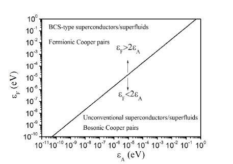
Figure 24: Phase diagram of the two fundamentally different types of Cooper pairs in superconductors and superfluids as a function of two characteristic parameters $\varepsilon_{A}$ and $\varepsilon_{F}$.

The bosonic nature of Cooper pairs becomes apparent when the Fermi energy is comparable with the double energy $2\varepsilon_{A}$ of the effective attraction between fermionic quasiparticles in high-$T_{c}$ cuprates, heavy-fermion and organic superconductors, liquid ³He and atomic Fermi gases (see Fig. 24). Specifically, Cooper pairs in the cuprates are bosons up to some overdoping level (corresponding to the QCP) above which the polaronic effects and related pseudogap disappear 158 . To illustrate this point, we apply the criterion (112) to the doped cuprates. For $\eta=\varepsilon_{\infty}/\varepsilon_{0}=0.02$, we found $E_{p}\simeq 0.081$ eV (see Table I). By choosing $\hbar\omega_{0}\simeq 0.07$ eV, we see that the criterion for bosonization of polaronic Cooper pairs is satisfied in doped cuprates at $\varepsilon_{F}\lesssim 2\varepsilon_{A}=2(E_{p}+\hbar\omega_{0})\simeq 0.3$ eV. This means that the bosonization of Cooper pairs is not expected in heavily overdoped cuprates with relatively large Fermi energies $\varepsilon_{F}\lesssim 0.4$ eV 206 . In these systems, Cooper pairs of quasi-free electrons (or holes) behave like fermions.

VI.2 B. The criteria for the bosonization of Cooper pairs depending on three characteristic parameters $\varepsilon_{A}$, $\varepsilon_{F}$ and $\Delta_{F}$

We now obtain the criteria for bozonization of Cooper pairs depending on three characteristic parameters of superconductors and superfluids. The bosonic nature of Cooper pairs in these systems can be specified by comparing the size of the Cooper pair $a_{c}$ with the mean distance $R_{c}$ between them. It may be important to identify which condensed matter systems characterized by the parameters $\varepsilon_{A}$, $\varepsilon_{F}$ and $\Delta_{F}$ are the conventional BCS-type ($s$-, $p$- or $d$-wave) superconductors (superfluids) or the unconventional Bose-type (i.e., non-BCS-type) superconductors (superfluids).

The size of a Cooper pair in a superconductor can be determined by using the uncertainty principle as 63

$$a_{c}\simeq\frac{\hbar}{2\Delta_{F}}\sqrt{\frac{\varepsilon_{F}}{2m^{*}_{F}}},$$ (113)

where $m^{*}_{F}$ is the effective mass of fermionic quasiparticles. The mean distance between Cooper pairs is determined by the expression

$$R_{c}\simeq(\frac{3}{4\pi n_{c}})^{1/3},$$ (114)

where $n_{c}$ is the concentration of Cooper pairs. The concentration of Cooper pairs $n_{c}$ depends on the attractive pairing interaction energy $\varepsilon_{A}$ (i.e., on the width of the energy layer near the Fermi surface). If $n$ is the total concentration of fermionic quasiparticles in the system, all of these quasiparticles (at small Fermi energies $\varepsilon_{F}\thicksim\varepsilon_{A}$) or some part of them, which is of order ($\varepsilon_{A}/\varepsilon_{F}$) $n$, may take part in the Cooper pairing. The concentration of fermionic quasiparticles $n$ enters into the expression for $\varepsilon_{F}$, which is given by

$$\varepsilon_{F}=\frac{\hbar^{2}(3\pi^{2}n)^{2/3}}{2m^{*}_{F}}.$$ (115)

The concentration of fermions, which take part in the Cooper pairing, is roughly defined as

$$n_{A}\simeq\frac{\varepsilon_{A}}{\varepsilon_{F}}n.$$ (116)

Using Eqs. (115) and (116), the expression for the concentration of Cooper pairs $n_{c}=n_{A}/2$ can be written as

$$n_{c}\simeq\frac{\varepsilon_{A}}{6\pi^{2}\varepsilon_{F}}\Big{(}\frac{2m^{*}_{F}\varepsilon_{F}}{\hbar^{2}}\Big{)}^{3/2}.$$ (117)

Then, the mean distance between Cooper pairs is determined from the relation

$$R_{c}\simeq\Big{(}\frac{9\pi\varepsilon_{F}}{2\varepsilon_{A}}\Big{)}^{1/3}\Big{(}\frac{\hbar^{2}}{2m_{F}^{*}\varepsilon_{F}}\Big{)}^{1/2}.$$ (118)

If the size of Cooper pairs $a_{c}$ is smaller than the mean distance $R_{c}$ between them, we deal with the non-overlapping Cooper pairs, which behave like bosons. Thus, it is quite clear that we deal with the unconventional Bose-type superconductors and superfluids if the condition $a_{c}<R_{c}$ is satisfied. Using the relations (117) and (118), the condition $R_{c}>a_{c}$ can be written as

$$\frac{\Delta_{F}}{\varepsilon_{F}}\gtrsim\Big{(}\frac{\varepsilon_{A}}{36\pi\varepsilon_{F}}\Big{)}^{1/3}.$$ (119)

The phase diagram of the two fundamentally different types of Cooper pairs in superconductors and superfluids obtained by using three characteristic parameters $\varepsilon_{A}$, $\varepsilon_{F}$ and $\Delta_{F}$ is shown in Fig. 25.

Figure 25: Phase diagram of the two fundamentally different types of Cooper pairs in superconductors and superfluids as a function of two characteristic ratios $\Delta_{F}/\varepsilon_{F}$ and $\varepsilon_{A}/\varepsilon_{F}$.

VI.3 1. The existence possibility of fermionic Cooper pairs in the BCS-type superconductors and superfluids

The theoretical interpretation of the unconventional superconductivity (superfluidity) in high-$T_{c}$ cuprates, heavy-fermion and organic systems and the superfluidity in liquid ³He as the BCS-like ($s$-, $p$- or $d$-wave) superconductivity (superfluidity) without clarifying the fermionic nature of Cooper pairs might be misleading. Therefore, researchers should first determine the fermionic nature of the Cooper pairs in the superconductors (superfluids) under consideration, and then they should discuss the possibility of the BCS- like ($s$-, $p$- or $d$-wave) superconductivity (superfluidity). The fermionic Cooper pairs in superconductors and superfluids would exist under the condition $a_{c}>R_{c}$, so that the criterion for the existence of such Cooper pairs can be written as

$$\frac{\Delta_{F}}{\varepsilon_{F}}\lesssim\Big{(}\frac{\varepsilon_{A}}{36\pi\varepsilon_{F}}\Big{)}^{1/3}.$$ (120)

We demonstrate that this criterion is well satisfied only in conventional superconductors and heavily overdoped cuprates with large Fermi energies $\varepsilon_{F}>>\varepsilon_{A}$. The maximum values of the energy gap $2\Delta_{F}$ in conventional superconductors are about $3\cdot 10^{-3}$ eV 1 . In these superconductors the Fermi energy $\varepsilon_{F}$ is about 10 eV and the phonon energy $\hbar\omega_{D}$ is of order $10^{-2}$ eV 1 . We see that the criterion (120) for the existence of fermionic Cooper pairs is actually satisfied very well in conventional BCS superconductors. Experimental results show that the values of $\Delta_{F}$ in overdoped cuprates vary from 0.010 eV to 0.020 eV 127 . In overdoped cuprates the carrier concentration $n$ is the order of $n\sim 10^{21}\rm{cm^{-3}}$ and the Fermi energy in the absence polaronic effects is determined from the relation (115) at $m^{*}_{F}=m_{e}$. Then the overdoped cuprates have relatively large Fermi energies $\varepsilon_{F}\gtrsim 0.4$ eV at $n\gtrsim 10^{21}\rm{cm^{-3}}$. In overdoped cuprates the cutoff energy $\varepsilon_{A}$ in Eq. (36) for the attractive electron-phonon interaction is replaced by the optical phonon energy $\hbar\omega_{0}\thicksim 0.05$ eV. For these systems, the criterion (120) is satisfied fairly well, since $\Delta_{F}/\varepsilon_{F}=0.05$ (at $\Delta_{F}=0.02$ eV and $\varepsilon_{F}=0.4$ eV ) and $(\varepsilon_{A}/36\pi\varepsilon_{F})^{1/3}\simeq 0.22$. However, underdoped, optimally doped and moderately overdoped cuprates may not satisfy this criterion at $m^{*}_{F}=m_{p}>m_{e}$, $\varepsilon_{A}=E_{p}+\hbar\omega_{0}$ and $n\lesssim 10^{21}\rm{cm^{-3}}$.

VI.4 2. The existence possibility of bosonic Cooper pairs in unconventional superconductors and superfluids

The bosonization of Cooper pairs is expected in unconventional superconductors and superfluids, in which the energy $\varepsilon_{A}$ of the effective attraction between fermions is comparable with Fermi energy $\varepsilon_{F}$, i. e., $\varepsilon_{A}\lesssim\varepsilon_{F}<<1$ eV. The criterion (119) allows us to determine the existence possibility of bosonic Cooper pairs in these systems.

The Fermi energy $\varepsilon_{F}$ of underdoped to overdoped cuprates determined from the relation (115) at $m^{*}_{F}=m_{p}=2m_{e}$ and $n\simeq(0.5-1.0)\cdot 10^{21}\rm{cm^{-3}}$ varies from 0.115 eV (for underdoped cuprates) to 0.182 eV (for overdoped cuprates). In these high-$T_{c}$ materials, the observed values of the energy gap $\Delta_{F}$ vary from 0.025 eV to 0.04 eV 43 and the quantity $\varepsilon_{A}$ will be determined by $E_{p}+\hbar\omega_{0}$, which is of order 0.1 eV. If we assume that $\Delta_{F}\simeq 0.04$ eV and $\varepsilon_{F}\simeq 0.115$ eV, we see that the criterion (119) for the existence of bosonic Cooper pairs is well satisfied in underdoped high-$T_{c}$ cuprates. By taking $\varepsilon_{A}=0.1$ eV and $\varepsilon_{F}\simeq 0.18$ eV for moderately overdoped cuprates, we can write the criterion (119) as $\Delta_{F}/\varepsilon_{F}\gtrsim 0.169$, which is satisfied for $\Delta_{F}>0.03$ eV.

The observed values of the pseudogap in heavy-fermion superconductors range from 0.001 eV 18 to 0.030 eV 193 . If we take $\varepsilon_{F}\simeq 0.03$ eV and $\Delta_{F}\simeq 0.01$ eV for these systems, then we shall see that the criterion (119) for bosonization of Cooper pairs is satisfied fairly well both in the case $\varepsilon_{A}<<\varepsilon_{F}$ and in the case $\varepsilon_{A}\lesssim\varepsilon_{F}$.

In organic superconductors the magnitude of the pseudogap is larger than 0.02 eV and the Fermi energy $\varepsilon_{F}$ is of order 0.1 eV. In these systems, the quantity $\varepsilon_{A}$ will be determined by $E_{p}+\hbar\omega_{0}$, which is of order 0.06 eV. Then the criterion (119) for the existence of bosonic Cooper pairs in organic superconductors at $\varepsilon_{A}/\varepsilon_{F}\simeq 0.6$ has the following form: $\Delta_{F}/\varepsilon_{F}\gtrsim(1/60\pi)^{1/3}$. We see that this criterion will be well satisfied when $\Delta_{F}/\varepsilon_{F}\simeq 0.2$.

We now determine the existence possibility of bosonic Cooper pairs in liquid ³He. If we take $\varepsilon_{F}\approx 10^{-4}$ eV and $\varepsilon_{A}\simeq 0.5\varepsilon_{F}$ for liquid ³He, we see that the criterion (119) for the existence of Cooper pairs in the normal state of ³He is satisfied at $\Delta_{F}\gtrsim 0.164\varepsilon_{F}$.

Thus, the above unconventional superconductors and superfluids are expected to be in the bosonic limit of Cooper pairs.

VII VII. Unusual superconducting and superfluid states of Bose liquids

London suggested 207 that the superfluid transition in liquid ⁴He is associated with the BEC phenomenon. However, the liquid ⁴He is strongly interacting Bose system and not an ideal Bose gas which undergoes a BEC. Later, Landau 208 showed that the frictionless flow of liquid ⁴He would be possible, if this liquid has the sound-like excitation spectrum satisfying the criterion for superfluidity. According to the BCS theory, all Cooper pairs in metals could occupy the same quantum state (by analogy with BEC), though they do not behave like Bose particles 203 ; 204 . However, unconventional superconductors and superfluids are in the bosonic limit of Cooper pairs, which in contrast to fermionic Cooper pairs in conventional superconductors may be looked upon in a way as composite bosons. Obviously, the BEC can take place in an ideal Bose gas but the resulting condensed system will not be superfluid by the Landau criterion.

We first discuss briefly the existing theories of superfluid Bose systems and then present the adequate microscopic theory of the Bose superfluids. Landau 208 developed a simple phenomenological theory of superfluidity which explains the behavior of the superfluid ⁴He at low temperatures not close to the $\lambda$-point. Later, Bogoliubov 209 took an important step towards a theoretical understanding of the superfluid state of ⁴He and proposed a microscopic theory of superfluidity, which is based on the so-called $c$-number condensate of a repulsive Bose gas. However, it turned out that the theory of a repulsive Bose-gas is unsuitable for studying the superfluid properties of ⁴He 73 ; 210 . Because the theory of repulsive Bose liquids or $c$-number-condensate theory 211 cannot explain a number of superfluid properties of ⁴He, such as the observed half-integral values of circulation 212 ; 213 , deviation of the specific heat from the phonon-like dependence 214 , the $\lambda$-like transition 30 , the condensed fraction $N_{B0}/N_{B}$ (where $N_{B0}$ is the number of Bose particles in the zero-momentum $k=0$ state, $N_{B}$ is the total number of Bose particles), and the depletion of the zero-momentum $k=0$ state 215 . Similar incorrect results are predicted by the pair condensate theories of Girardeau and Arnowitt and others (see Ref. 216 ). As emphasized first by Luban 210 and then by Evans and Imry 73 , these inconsistencies in the theory of repulsive Bose liquids are caused by using the unnecessary Bogoliubov approximation (replacing the zero-momentum creation and annihilation operators by $c$-numbers).

Other microscopic theories of a nonideal Bose gas have been proposed by Valatin and Butler 217 , Luban 210 , and Evans and Imry 73 without using the Bogoliubov approximation. Although the approaches to the problem of superfluid condensation in a nonideal Bose gas proposed in Refs. 210 ; 217 are different from the $c$-number condensate theory of Bogoliubov, these approaches led to the Bogoliubov result in the case of a predominantly repulsive interaction. Also, the treatment of the zero-momentum ($k=0$) terms in the Valatin-Butler theory 217 led to the inconsistencies, as pointed out by Evans and Imry 73 . The Luban’s theory of superfluidity is tenable near $T_{c}$ which is redefined temperature $T_{BEC}$ of an ideal Bose gas (with the renormalized mass of bosons). The phase transition in a nonideal Bose gas at $T_{c}$ predicted by this theory is similar to the phase transition in an ideal Bose gas, which is not $\lambda$-like transition observed in liquid ⁴He. It is important to note that the Luban’s theory at $T\geq T_{c}$ is the boson analog of Landau’s Fermi-liquid theory. A more consistent numerical approach to the theory of a Bose-liquid was developed in Refs. 73 and 218 by taking into account both repulsive and attractive parts of interboson interaction. This pairing theory of the Bose superfluid is developed by analogy with the BCS pairing theory of fermions and is based on the concept of the pair condensation in an attractive Bose gas. Further, a more general approach to the theory of a superfluid Bose-liquid was proposed by Dorre et al. 211 . This approach combines the $c$-number condensate theory 209 ; 219 and boson pairing theory 73 ; 218 (i.e. the boson analog of the BCS theory). The pair BEC into the $k=0$ state described in the pairing theories of bosons 73 ; 211 seems to be unphysical, as argued also in Ref. 220 . The validity of the $c$-number condensate theory 211 is controversial as it was noted by the authors themselves, and by Evans 221 . Moreover, Dorre et al. 211 assert that their (including also Evans and co-workers 73 ; 218 ) pairing theory is also irrelevant to the superfluid state of ⁴He. It seems that the basic results of Ref. 211 , such as the gapless energy spectrum up to $T_{c}$ and the large condensate fraction $N_{B0}/N_{B}\simeq 0.93-0.96$ (see also Ref. 221 ) are contradictory and at variance with the observed behavior of superfluid ⁴He. Actually, in superfluid ⁴He the observed condensed fraction $n_{B0}=N_{B0}/N_{B}$ in the $k=0$ state is found to be small, i.e., $n_{B0}\simeq 0.1$ at $T=0$ 215 . In the alternative models, the so-called single particle and pair condensations in an interacting Bose-gas have been studied at $T=0$. Such models of a Bose-liquid with the interboson interaction potential, which has both repulsive and attractive parts, have been proposed in Refs. 222 ; 223 . In these models, the possibility of single particle and pair condensations of attracting bosons has not been studied for the important temperature range $0<T\leq T_{c}$. Also, the possibility of single particle and pair condensations in a purely attractive Bose system has been discussed in Ref. 220 at $T=0$.

After the discovery of the layered high-$T_{c}$ cuprate superconductors, a 2D model of an interacting Bose gas adapted to a 2D boson-like holon gas has been discussed in Refs. 224 ; 225 , where the superconducting transition temperature $T_{c}$ (i.e. the onset temperature of pair condensation) of such exotic bosons was obtained only in the weak coupling limit. Further, it was argued 22 ; 50 ; 51 that the single particle and pair condensations of bosonic of Cooper pairs can occur in high-$T_{c}$ cuprates and other unconventional superconductors and superfluids. The number of the interacting fermions in the energy layer of width $\varepsilon_{A}$ around the Fermi surface taking part in the Cooper pairing below the characteristic temperature $T^{*}$ is determined from Eq. (IV.3). The number of excited Fermi components of Cooper pairs below $T^{*}$ (e.g., at $T\simeq 0.9T^{*}$ or even at $T\simeq 0.95T^{*}$) determined from the equation

$$n_{p}^{*}=2\sum_{k}u_{k}f_{C}(k)=\frac{\sqrt{2m_{ab}^{2}m_{c}}}{2\pi^{2}\hbar^{3}}\times$$

$$\times\int\limits_{-\varepsilon_{A}}^{\varepsilon_{A}}\left(1+\frac{\xi}{E}\right)\frac{(\xi+\varepsilon_{F})^{1/2}}{\exp[E/k_{B}T]+1}d\xi$$ (121)

becomes rather small in comparison with $n_{c}=n_{B}$. Actually, the number of bosonic Cooper pairs $n_{c}$ somewhat below $T^{*}$ becomes much larger than $n_{p}^{*}$ and remains almost unchanged when the temperature decreases down to $T_{c}$. Thus, fermions (which are products of the thermal dissociation of Cooper pairs) and bosonic Cooper pairs residing in the energy layer of width $\varepsilon_{A}$ near the Fermi surface are essentially decoupled just like the spin-charge separation in RVB model 35 ; 56 ; 75 .

From what has been already stated, it follows that the possible superfluid states and basic superfluid properties of Bose liquids were not established as functions of interboson interaction strength or coupling constant and temperature for the complete temperature range $0\leq T\leq T_{c}$, and the existing microscopic theories were not in a satisfactory state for understanding all the superfluid properties of ⁴He and other Bose-liquids. In this section, we construct a quantitative, predictive microscopic theory of the genuine superfluidity and superconductivity of Bose liquids. In this theory the pair boson Hamiltonian and realistic BCS-like approximation for the interboson interaction potential are used to solve the self-consistent set of integral equations not only for $T=0$ and weak interboson coupling, but also for the temperature range $0<T\leq T_{c}$ and arbitrary interboson coupling strengths. We show that the coherence parameter (i.e. superfluid order parameter) will appear at a $\lambda$-like transition temperature, $T_{c}=T_{\lambda}$, which is also marks the onset of the superfluid condensation of attracting bosons.

In the following, we describe the essentials of the complete and detailed microscopic theory of superfluid states of 3D and 2D Bose liquids.

VII.1 A. Pair Hamiltonian model of an attractive Bose system

We consider a system of $N_{B}$ Bose particles of mass $m_{B}$ and density $\rho_{B}=N_{B}/\Omega$ (where $\Omega$ is the volume of the system) and start from the boson analog of the BCS-like Hamiltonian. These Bose particles repel one another at small distances between them and their net interaction is attractive at large distances. Therefore, in the pair Hamiltonian of an interacting Bose gas, we take explicitly into account both the short-range repulsive (preventing collapse of an attractive Bose system) and long-range attractive interboson interactions.

The boson analog of the BCS-like Hamiltonian, which describes the pair interaction between Bose particles, is similar to Eq. (III.5). In the mean-field approximation, the pair Hamiltonian of the interacting Bose gas can be written as

$$H_{B}=\sum_{\vec{k}}[\tilde{\varepsilon}_{B}(k)c^{+}_{\vec{k}}c_{\vec{k}}-\Delta_{B}(k)(c^{+}_{\vec{k}}c^{+}_{-\vec{k}}+c_{-\vec{k}}c_{\vec{k}}-B^{*}_{\vec{k}})],$$

where $\tilde{\varepsilon}_{B}(\vec{k})=\varepsilon(k)-\mu_{B}+V_{B}(0)\rho_{B}+\chi_{B}(\vec{k})$ is the Hartree-Fock quasiparticle energy, $\varepsilon(k)=\hbar^{2}k^{2}/2m_{B}$, $\chi_{B}(\vec{k})=(1/\Omega)\sum_{\vec{k}^{\prime}}V_{B}(\vec{k}-\vec{k}^{\prime})n_{B}(\vec{k})$, $\Delta_{B}(\vec{k})=-(1/\Omega)\sum_{\vec{k}^{\prime}}V_{B}(\vec{k}-\vec{k}^{\prime})\langle c_{-\vec{k}^{\prime}}c_{\vec{k}^{\prime}}\rangle$ is the coherence parameter, $n_{B}(\vec{k})=\langle c^{{\dagger}}_{\vec{k}}c_{\vec{k}}\rangle$ is the particle number operator, $\rho_{B}=(1/\Omega)\sum_{\vec{k}^{\prime}}n_{B}(\vec{k}^{\prime})$, $\mu_{B}$ is the chemical potential of free bosons, $c^{{\dagger}}_{\vec{k}}(c_{\vec{k}})$ is the creation (annihilation) operator of bosons with the wave vector $\vec{k}$, $B^{*}_{\vec{k}}=<c^{+}_{\vec{k}}c^{+}_{-\vec{k}}>$, $V_{B}(\vec{k}-\vec{k}^{\prime})$ is the interboson interaction potential.

The Hamiltonian (VII.1) is diagonalized by using the Bogoliubov transformations of Bose operators 209

$$c_{\vec{k}}=u_{k}\alpha_{\vec{k}}-v_{k}\alpha^{+}_{\vec{k}},\ c^{+}_{\vec{k}}=u_{k}\alpha^{+}_{\vec{k}}-v_{k}\alpha_{-\vec{k}},$$

$$c_{-\vec{k}}=u_{k}\alpha_{-\vec{k}}-v_{k}\alpha^{+}_{\vec{k}},\ c^{+}_{-\vec{k}}=u_{k}\alpha^{+}_{-\vec{k}}-v_{k}\alpha_{\vec{k}},$$ (123)

where $\alpha_{\vec{k}}$ and $\alpha^{+}_{\vec{k}}$ are the new annihilation and creation operators of Bose quasiparticles, which satisfy the Bose commutation rules $[\alpha_{\vec{k}},\alpha^{+}_{\vec{k}}]=1$ and $[\alpha_{\vec{k}},\alpha_{\vec{k}}]=[\alpha^{+}_{\vec{k}},\alpha^{+}_{\vec{k}}]=0$, $u_{k}$ and $v_{k}$ are the real functions satisfying the condition

$$u^{2}_{k}-v^{2}_{k}=1.$$ (124)

Substituting Eq. (VII.1) into Eq. (VII.1) and taking into account Eq. (124), we obtain the diagonalized Hamiltonian

$$H_{B}=W_{0}+\sum_{\vec{k}}E_{B}(\vec{k})(\alpha^{+}_{\vec{k}}\alpha_{\vec{k}}+\alpha^{+}_{-\vec{k}}\alpha_{-\vec{k}}),$$ (125)

where

$$W_{0}=\sum_{\vec{k}}\Big{[}E_{B}(\vec{k})-\tilde{\varepsilon}_{B}(\vec{k})+\Delta_{B}(\vec{k})B^{*}_{\vec{k}}\Big{]}$$ (126)

is the ground state energy of a Bose-liquid, and $E_{B}(\vec{k})$ is the excitation spectrum of interacting bosons given by

$$E_{B}(\vec{k})=\sqrt{\tilde{\varepsilon}^{2}_{B}(\vec{k})-\Delta^{2}_{B}(\vec{k})},$$ (127)

which is different from the BCS-like excitation spectrum of interacting fermions.

The coherence parameter $\Delta_{B}(\vec{k})$ would represents the superfluid (or superconducting) order parameter appearing at a certain mean-field temperature $T_{c}$ which in turn represents the onset temperature of the superfluid phase transition in Bose liquids. Using the transformation of Bose operators ($c^{+}_{\vec{k}}$ and $c_{\vec{k}}$), Eq. (VII.1) together with Eq. (124), the parameters $\Delta_{B}(\vec{k})$, $\rho_{B}$ and $\chi_{B}(\vec{k})$ are determined from simultaneous equations

$$\Delta_{B}(k)=-\frac{1}{\Omega}\sum_{\vec{k^{\prime}}}V_{B}(\vec{k}-\vec{k}^{\prime})\frac{\Delta_{B}(\vec{k}^{\prime})}{2E_{B}(\vec{k}^{\prime})}\coth\frac{E_{B}(\vec{k}^{\prime})}{2k_{B}T},$$

$$N_{B}=\sum_{\vec{k}}n_{B}(\vec{k})=\sum_{k^{\prime}}\left[\frac{\tilde{\varepsilon}_{B}(\vec{k})}{2E_{B}(\vec{k})}\coth\frac{E_{B}(\vec{k})}{2k_{B}T}-\frac{1}{2}\right],$$

$$\chi_{B}(\vec{k})=\frac{1}{\Omega}\sum_{\vec{k^{\prime}}}V_{B}(\vec{k}-\vec{k}^{\prime})\left[\frac{\tilde{\varepsilon}_{B}(\vec{k}^{\prime})}{2E_{B}(\vec{k}^{\prime})}\coth\frac{E_{B}(\vec{k}^{\prime})}{2k_{B}T}-\frac{1}{2}\right],$$

by means of their self-consistent solutions.

We shall now see that the gapless excitation spectrum of a superfluid Bose-liquid is quite different from the gapless excitation spectrum of a BCS-like Fermi-liquid. As seen from Eq. (127), if $\tilde{\mu_{B}}=-\mu_{B}+V_{B}(0)\rho_{B}+\chi_{B}(0)=|\Delta_{B}(0)|$, then the excitation spectrum of interacting bosons becomes gapless for $k=0$ and $k^{\prime}=0$. Therefore, for obtaining the self-consistent solutions of Eqs. (VII.1)-(VII.1), the $k=0$ and $k^{\prime}=0$ terms in the summation of these equations should be considered separately according to the procedure proposed in Ref. 73 as

$$\Delta_{B}(\vec{k})=-V_{B}(\vec{k})\rho_{B0}sign(\Delta_{B}(0))$$

$$-\frac{1}{\Omega}\sum_{\vec{k}^{\prime}\neq 0}V_{B}(\vec{k}-\vec{k}^{\prime})\frac{\Delta_{B}(\vec{k}^{\prime})}{2E_{B}(\vec{k}^{\prime})}\coth\frac{E_{B}(\vec{k}^{\prime})}{2k_{B}T},$$ (131)

$$N_{B}=N_{B0}+\sum_{\vec{k}\neq 0}\left[\frac{\tilde{\varepsilon}_{B}(\vec{k})}{2E_{B}(\vec{k})}\coth\frac{E_{B}(\vec{k})}{2k_{B}T}-\frac{1}{2}\right],$$ (132)

$$\chi_{B}(\vec{k})=V_{B}(\vec{k})\rho_{B0}+\frac{1}{\Omega}\sum_{k^{\prime}\neq 0}V_{B}(\vec{k}-\vec{k}^{\prime})\times$$

$$\times\left[\frac{\tilde{\varepsilon}_{B}(\vec{k^{\prime}})}{2E_{B}(\vec{k}^{\prime})}\coth\frac{E_{B}(\vec{k}^{\prime})}{2k_{B}T}-\frac{1}{2}\right],$$ (133)

where $\rho_{B0}=N_{B0}/\Omega$ is the density of Bose particles with $k=0$.

In order to simplify the solutions of Eqs. (VII.1)-(VII.1), the pair interboson interaction potential, which has a repulsive part $V_{BR}$ and an attractive part $V_{BA}$, may be chosen in a simple separable form 51

$$V_{B}(\vec{k}-\vec{k}^{\prime})=\left\{\begin{array}[]{lll}V_{BR}-V_{BA}&\textrm{if}\>0\leq\varepsilon(k),\>\varepsilon(k^{\prime})<\xi_{BA},\\ V_{BR}&\textrm{if}\>\xi_{BA}\leq\varepsilon(k)\>\textrm{or}\>\varepsilon(k^{\prime})<\xi_{BR},\\ 0&\textrm{if}\>\varepsilon(k),\>\varepsilon(k^{\prime})>\xi_{BR},\end{array}\right.$$ (137)

where $\xi_{BA}$ and $\xi_{BR}$ are the cutoff energies for attractive and repulsive parts of the $V_{B}(\vec{k}-\vec{k}^{\prime})$, respectively.

This approximation allows us to carry out the calculation thoroughly and so it gives us a new insight into the superfluididty of a Bose-liquid. Further, we assume that $\xi_{BR}>>\xi_{BA}>>\tilde{\mu}_{B}=-\mu_{B}+V_{B}(0)\rho_{B}+\chi_{B}(0)\sim\Delta_{B}\sim k_{B}T_{c}$ and $\tilde{\mu}_{B}$ is essentially positive. The cutoff parameter $\xi_{BA}$ characterizes the thickness of the condensation layer including almost all Bose particles. Therefore, the main contribution to the sums in Eqs. (VII.1)-(VII.1) comes from those values of $k$ less than $k_{A}$, whereas the large values of $k>k_{A}$ give small corrections that may be neglected. Here we note that not all the bosons in the system can undergo a superfluid condensation, but only their attractive part with the particle density $\rho_{B}$ undergoes a phase transition to the superfluid state.

VII.2 B. Two distinct superfluid states of a 3D Bose-liquid

We now consider the possible superfluid states of a 3D Bose liquid. In so doing, we show that the analytical and numerical solutions of Eqs. (VII.1)-(VII.1) obtained using the model potential (137) allow us to examine closely the possibility of the existence of two distinct superfluid condensates and superfluid states arising in attractive Bose systems.

VII.3 1. Distinctive single particle and pair condensations of attracting bosons at $T=0$

Replacing the summation in Eqs. (VII.1)-(VII.1) over $\vec{k}$ and $\vec{k^{\prime}}$ by an integration over $\varepsilon$ and making elementary transformations, we obtain the following equations for determination of the critical values of $\rho_{B}$ and $\tilde{\mu}_{B}$ at which the quasiparticle excitation spectrum $E_{B}(k)=\sqrt{(\varepsilon(k)+\tilde{\mu}_{B})^{2}-\Delta^{2}_{B}}$ becomes gapless and the superfluid single particle condensation of attracting bosons sets in (see Appendix B):

$$|\tilde{\mu}_{B}|=\frac{\xi_{BA}}{2}\left(\frac{\gamma_{B}^{*2}-1}{2\gamma_{B}}\right)^{2},$$ (139)

$$\rho_{B}=\frac{D_{B}\xi_{BA}^{3/2}}{48}\left(\frac{\gamma_{B}^{*2}-1}{\gamma_{B}}\right)^{3},$$ (140)

where $\gamma_{B}^{*}$ is a critical value of the interboson coupling constant $\gamma_{B}=\tilde{V}_{B}D_{B}\sqrt{\xi_{BA}}$.

The excitation spectrum $E_{B}(k)$ of interacting bosons has a finite energy gap $E_{B}(0)=\Delta_{g}=\sqrt{\tilde{\mu}_{B}^{2}-\Delta^{2}_{B}}$ at $\gamma_{B}>\gamma^{*}_{B}$ and becomes gapless (phonon-like) at $\gamma_{B}\leq\gamma^{*}_{B}$. Therefore, such a quasiparticle excitation spectrum satisfies the Landau criterion for superfluidity at $k\rightarrow 0$. If $E_{B}(0)>0$, $2E_{B}(0)$ is the minimum energy needed to break a condensed boson pair 220 . The pair condensation of bosons occurs if the attractive interaction between them is strong enough to produce a bound state. As seen from Eqs. (139) and (140), the formation of a boson pair with the binding energy $2\Delta_{g}$ is possible only at $\gamma_{B}>\gamma^{*}_{B}>1$. This means that the superfluid pair condensation of bosons sets in at $\gamma_{B}>\gamma^{*}_{B}$ and the existence of a finite energy gap $\Delta_{g}$ guarantees stability of a superfluid pair condensate, as noted in Ref. 220 . Increasing the density of bosons opposes pair formation and the energy gap $\Delta_{g}$ vanishes at $\gamma_{B}\leqslant\gamma_{B}^{*}$. The single particle condensation of bosons sets in just at $\gamma_{B}=\gamma^{*}_{B}$ at which boson pairs dissociate. The value of $\tilde{\mu}_{B}$ at $\gamma_{B}\leqslant\gamma^{*}_{B}$ is equal to (see Appendix B)

$$\tilde{\mu}_{B}=\Delta_{B}=2.88k_{B}T_{BEC}.$$ (141)

From Eqs. (139) and (141), it follows that the critical value of $\gamma_{B}=\gamma_{B}^{*}$ is determined from the relation

$$\gamma^{*}_{B}=2.404\sqrt{\frac{k_{B}T_{BEC}}{\xi_{BA}}}+\sqrt{1+\frac{5.779k_{B}T_{BEC}}{\xi_{BA}}}.$$ (142)

For $\gamma_{B}\leqslant\gamma^{*}_{B}$, the fraction of condensed bosons in the $k=0$ state $n_{B0}=\rho_{B0}/\rho_{B}$ is determined as a function of $\gamma_{B}$ from the following equations (see Appendix B)

$$3(\rho_{B}-\rho_{B0})=\sqrt{2}\tilde{\mu}_{B}^{3/2}D_{B},$$ (143)

$$\rho_{B0}=\frac{D_{B}\tilde{\mu}_{B}\sqrt{\xi_{BA}}}{\gamma_{B}}\left[1-\gamma_{B}\left(\sqrt{1+\frac{2\tilde{\mu}_{B}}{\xi_{BA}}}-\sqrt{\frac{2\tilde{\mu}_{B}}{\xi_{BA}}}\right)\right],$$

From these equations we find

$$n_{B0}=\frac{g_{0}}{g_{0}+\gamma_{B}\sqrt{5.76k_{B}T_{BEC}/\xi_{BA}}},$$ (145)

where $g_{0}=3[1-\gamma_{B}(\sqrt{1+5.76k_{B}T_{BEC}/\xi_{BA}}-\sqrt{5.76k_{B}T_{BEC}/\xi_{BA}})]$.

It follows from Eq. (145) that the single particle condensate ($n_{B0}\neq 0$) will appear when the quasiparticle excitation spectrum $E_{B}(k)$ becomes gapless at $\gamma_{B}=\gamma^{*}_{B}\simeq 1.5-2.0$ for $\xi_{BA}/k_{B}T_{BEC}=10-30$. At $\gamma_{B}\rightarrow 0$, all bosons will condense into the $k=0$ state, i.e., $n_{B0}\rightarrow 1$. In this case we have deal with the usual BEC of an ideal Bose-gas. As can be seen from Fig. 26, the condensate fraction $n_{B0}$ in these systems decreases with increasing $\gamma_{B}$ and becomes zero at $\gamma_{B}\geq\gamma^{*}_{B}$.

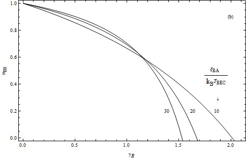
Figure 26: Dependence of the condensate fraction on the coupling constant $\gamma_{B}$ in 3D Bose superfluids at $T=0$ and $\xi_{BA}/k_{B}T_{BEC}$=10, 20 and 30.

The ground state energy $W_{0}$ of a 3D Bose-liquid at $T=0$ can be evaluated using the relation (126) and model potential (142). The expectation value of the product of operators $c^{+}_{k}c^{+}_{-k}$ is defined as

$$B^{*}_{k}=-\frac{\Delta_{B}(k)}{2E_{B}(k)},$$ (146)

Substituting now this expression into Eq. (126) and replacing the summation in this equation by an integration from 0 to $\xi_{BA}$, we obtain

$$W_{0}=D_{B}\Omega\Big{[}-\int_{0}^{\xi_{BA}}\sqrt{\varepsilon}(\varepsilon+\tilde{\mu}_{B})d\varepsilon+$$

$$+\int_{0}^{\xi_{BA}}\sqrt{\varepsilon}\sqrt{(\varepsilon+\tilde{\mu}_{B})^{2}-\Delta_{B}^{2}}d\varepsilon-$$

$$-\frac{\Delta^{2}_{B}}{2}\int\limits_{0}^{\xi_{BA}}\frac{\sqrt{\varepsilon}d\varepsilon}{\sqrt{(\varepsilon+\tilde{\mu}_{B})^{2}-\Delta_{B}^{2}}}\Big{]}.$$

Evaluating the integrals in Eq. (VII.3), we find (see Appendix B)

$$W_{0}\simeq-2D_{B}\Delta^{2}_{B}\xi^{1/2}_{BA}\Omega.$$

It follows from Eq. (VII.3) that the energy of a 3D Bose-liquid in the superfluid state (at $T<T_{c}$ and $\Delta_{B}>0$) is lower than its energy in the normal-state given by $W_{0}(\Delta_{B}=0)=0$.

Thus, the superfluid condensation energy of attracting 3D bosons is defined as

$$E_{S}=W_{0}(\Delta_{B}=0)-W_{0}(\Delta_{B}>0)=2D_{B}\Delta^{2}_{B}\xi^{1/2}_{BA}\Omega.$$

VII.4 2. Distinctive single particle and pair condensations of attracting bosons at $T\neq 0$

We now examine the numerical and analytical solutions of Eqs. (VII.1)-(VII.1) obtained using the model potential Eq. (137) for the case $T\neq 0$ and show that the quasiparticle excitation spectrum $E_{B}(k)$ satisfying the Landau criterion for superfluidity has a finite energy gap $\Delta_{g}>0$ above some characteristic temperature $T^{*}_{c}$ and becomes gapless below $T^{*}_{c}<T_{c}$ (at $\gamma_{B}<\gamma^{*}_{B}$) or $T^{*}_{c}<<T_{c}$ (at $\gamma_{B}<<\gamma^{*}_{B}$). If $\gamma_{B}>\gamma_{B}^{*}$ and $\Delta_{g}>0$ the numerical and analytical solutions of Eqs. (VII.1)-(VII.1) exhibit a second-order phase transition from the normal state to superfluid state (i.e., pair-condensed state) at $T=T_{c}$ in a 3D Bose-liquid without any feature of the order parameter $\Delta_{B}(T)$ below $T_{c}$ (see Fig. 27a). If $\gamma_{B}\leq\gamma_{B}^{*}$, such solutions of Eqs. (VII.1)-(VII.1) exhibit two successive phase transitions to distinct superfluid states with decreasing $T$. A second-order phase transition occurs first to the superfluid state of pair boson condensate at $T_{c}$. Further, a first-order phase transition to the superfluid state of single-particle boson condensate occurs at lower temperatures ($T=T^{*}_{c}$) at which the energy gap $\Delta_{g}$ vanishes. A key point is that the pair condensation of attracting bosons occurs first at $T_{c}$ and then their single particle condensation sets in at a temperature $T^{*}_{c}$ lower than $T_{c}$. As $T$ approaches $T^{*}_{c}$ from above, both the $\tilde{\mu}_{B}(T)$ the $\Delta_{B}(T)$ suddenly increases at $T^{*}_{c}$. Therefore, the order parameter $\Delta_{B}(T)$ shows the pronounced (at $\gamma_{B}<<\gamma^{*}_{B}$) and in some cases not very pronounced (at $\gamma_{B}<\gamma^{*}_{B}$) kink-like behavior near $T^{*}_{c}$ (see Figs. 27b and 27c).

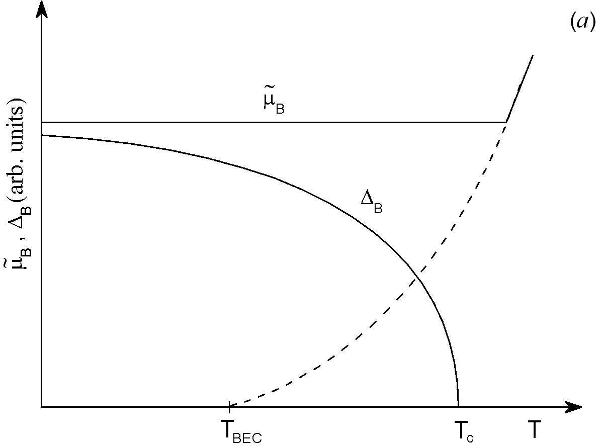
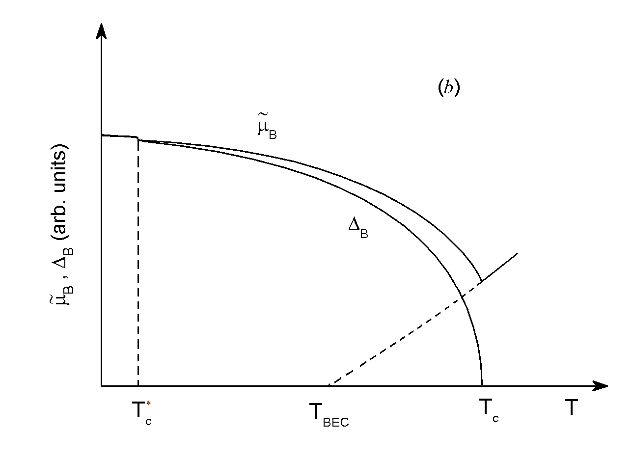
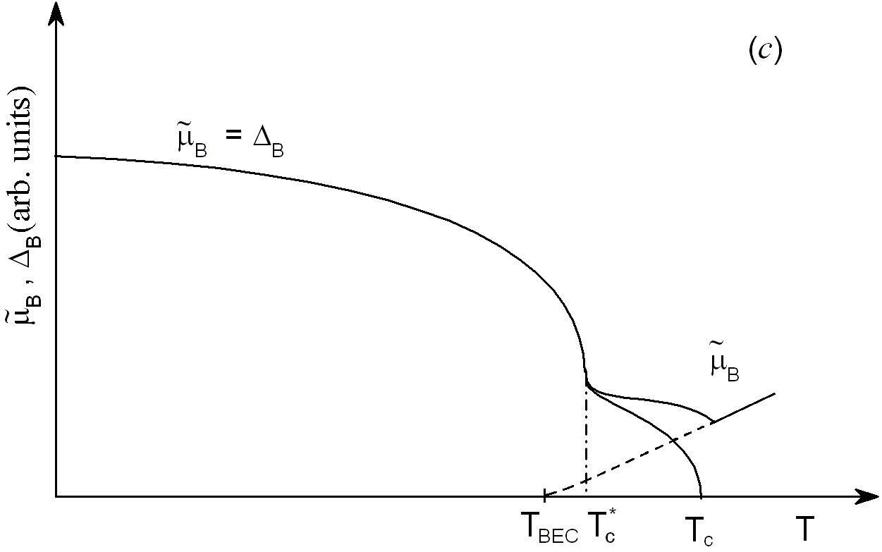
Figure 27: Temperature dependences of the chemical potential $\tilde{\mu}_{B}$ and coherence parameter $\Delta_{B}$ of a 3D Bose-liquid (solid curves), for different coupling constants $\gamma_{B}$: (a) for $\gamma_{B}>\gamma^{*}_{B}$; (b) for $\gamma_{B}<\gamma^{*}_{B}$ and (c) for $\gamma_{B}<<\gamma^{*}_{B}$. Dashed curves indicate temperature dependences of the chemical potential of an ideal 3D Bose gas.

In limit cases, the solutions of Eqs. (VII.1)-(VII.1) may be obtained analytically. For $T\leq T^{*}_{c}<<T_{c}$, we use Eqs. (VII.1)-(VII.1) to study the behavior of $n_{B0}(T)$, $\tilde{\mu}_{B}(T)$ and $\Delta_{B}(T)$.

Figure 28: Variation of the ratio $T^{*}_{c}/T_{c}$ with coupling constant $\gamma_{B}$ for $\gamma_{B}<\gamma^{*}_{B}\simeq 1.69$, $\tilde{\mu}_{B}\simeq k_{B}T_{c}$ and $\tilde{\mu}_{B}/\xi_{A}=0.15$

From these equations it follows (see Appendix C) that

$$\frac{2\rho_{B0}(T)}{D_{B}}\simeq\frac{2\rho_{B}}{D_{B}}-\frac{2}{3}\sqrt{2}\tilde{\mu}_{B}^{3/2}-\frac{(\pi k_{B}T)^{2}}{3\sqrt{2\tilde{\mu}_{B}}}$$ (150)

$$-\rho_{B0}(T)\simeq\tilde{\mu}_{B}D_{B}\Big{[}\sqrt{\xi_{BA}+2\tilde{\mu}_{B}}-$$

$$-\sqrt{2\tilde{\mu}_{B}}+\frac{(\pi k_{B}T)^{2}}{6\sqrt{2}\tilde{\mu}_{B}^{3/2}}-\frac{\sqrt{\xi_{BA}}}{\gamma_{B}}\Big{]},$$ (151)

where $\rho_{B0}(T)=0$ for $T\geqslant T^{*}_{c}$.

The values of $T_{c}^{*}(\gamma_{B})$ and $n_{B0}(T)$ can be obtained from Eqs. (150) and (VII.4). From Eq. (150) it is clear that $\rho_{B0}(0)=\rho_{B}-(2\tilde{\mu}_{B})^{3/2}/6$. At $T<T^{*}_{c}<<T_{c}$, we obtain from Eq. (150) the following expression for $n_{B0}(T)$:

$$n_{B0}(T)=n_{B0}(0)[1-gT^{2}],$$ (152)

where $g=m_{B}/12\rho_{B0}(0)\hbar^{3}v_{c}$, $v_{c}=\sqrt{\Delta_{B}/m_{B}}$ is the sound velocity. Such an expression for $n_{B0}(T)$ was also obtained in the framework of the phenomenological approach 215 ; where, however, instead of $\rho_{B0}(0)$ stands $\rho_{B}$ that correspond to the BEC of an ideal Bose gas. Both $n_{B0}(T)$ and $\Delta_{B}(T)$ are proportional to $T^{*}_{c}-T$ near $T^{*}_{c}(<<T_{c})$. One can assume that $\tilde{\mu}_{B}$ is of order $k_{B}T_{c}$. Then we can estimate the ratio $T^{*}_{c}/T_{c}$ using Eq. (VII.4) and argue that the magnitude of $T_{c}^{*}/T_{c}$ decreases with increasing $\gamma_{B}$ (Fig. 28). Now, we consider the other limit case $\gamma_{B}<<\gamma^{*}_{B}$ (i.e, a special case of the Bose systems, in which the interboson interactions are relatively weak and the characteristic temperature $T^{*}_{c}$ is comparatively close to $T_{c}$) and argue that the energy gap in $E_{B}(k)$ vanishes somewhat below $T_{c}$ (Fig. 27c). Assuming that $\Delta_{B}<\tilde{\mu}_{B}<<k_{B}T_{c}$ for $T^{*}_{c}<T<T_{c}$, the solution of Eqs. (VII.1)- (VII.1) may be found analytically, and, upon approaching $T_{c}$ we obtain (see Appendix C)

$$2.612\sqrt{\pi}(k_{B}T_{BEC})^{3/2}\simeq$$

$$\sqrt{\pi}(k_{B}T)^{3/2}\left[2.612-2\sqrt{\frac{\pi\tilde{\mu}_{B}}{k_{B}T}}\left(1-\frac{\Delta_{B}^{2}}{8\tilde{\mu}_{B}^{2}}\right)\right],$$ (153)

$$\frac{1}{\gamma_{B}}\simeq\frac{\pi k_{B}T}{2\sqrt{\tilde{\mu}_{B}\xi_{BA}}}\left(1+\frac{\Delta_{B}^{2}}{8\tilde{\mu}_{B}^{2}}\right),$$ (154)

from which at $T=T_{c}$ and $\Delta_{B}=0$, we obtain

$$2.612\sqrt{\pi}(k_{B}T_{c})^{3/2}=2.612\sqrt{\pi}(k_{B}T_{BEC})^{3/2}+$$

$$+\pi^{2}\gamma_{B}(k_{B}T_{c})^{3/2}\sqrt{k_{B}T_{c}/\xi_{BA}}.$$

This equation yields

$$T_{c}\simeq\frac{T_{BEC}}{[1-(\pi^{3/2}/2.612)\gamma_{B}\sqrt{k_{B}T_{c}/\xi_{BA}}]^{2/3}}.$$ (156)

It is interesting to examine the behavior of $\tilde{\mu}_{B}(T)$ and $\Delta_{B}(T)$ near $T_{c}$. According to Eqs. (VII.4) and (154), the temperature dependences of $\Delta_{B}$ and $\tilde{\mu}_{B}$ near $T_{c}$ are determined from the following relations (see Appendix C)

$$\tilde{\mu}_{B}(T)\simeq\tilde{\mu}_{B}(T_{c})\left[1+a\left(T_{c}-T\right)^{0.5}\right],$$ (157)

$$\Delta_{B}\simeq 2\tilde{\mu}_{B}(T_{c})\sqrt{a}\left(T_{c}-T\right)^{0.25},$$ (158)

where $a=2(c_{0}\gamma_{B}T_{c})^{-0.5}(\xi_{BA}/k_{B}T_{c})^{0.25}$.

The prediction of the behavior of $\tilde{\mu}_{B}(T)$, $\Delta_{B}(T)$ and $n_{B0}(T)$ in the vicinity of $T^{*}_{c}$ is also interesting. When $T$ approaches $T^{*}_{c}$ from below, the solutions of Eqs. (VII.1)-(VII.1) at $\tilde{\mu}_{B}(T^{*}_{c})<<k_{B}T^{*}_{c}$ are similar to the above presented solutions of Eqs. (VII.1)-(VII.1) at $T\rightarrow T_{c}$. Then the temperature dependences of $\tilde{\mu}_{B}$, $\Delta_{B}$ and $n_{B0}$ near the temperature $T^{*}_{c}$ are determined from the following relations (see Appendix C)

$$\tilde{\mu}_{B}(T)\simeq\tilde{\mu}_{B}(T^{*}_{c})\left[1+b(T^{*}_{c}-T)^{0.5}\right],$$ (159)

$$n_{B0}(T)\simeq\frac{b\gamma_{B}D_{B}(\pi k_{B}T^{*}_{c})^{2}}{2\rho_{B}\sqrt{2\xi_{BA}}}\left(T^{*}_{c}-T\right)^{0.5},$$ (160)

where $b=(c_{0}\gamma_{B}T^{*}_{c})^{-0.5}(\xi_{BA}/k_{B}T^{*}_{c})^{0.25}$.

According to Eqs. (159) and (160), the $\tilde{\mu}_{B}(T)$ and $\Delta_{B}(T)$ have the kink-like temperature dependences around $T^{*}_{c}(<T_{c})$. At $\tilde{\mu}_{B}(T)/k_{B}T_{c}^{*}<<1$ and $\rho_{B0}=0$, the characteristic temperature $T^{*}_{c}$ of the first order phase transition in the superfluid state of a $3D$ Bose-liquid is determined from the following equations (see Appendix C)

$$\frac{2\rho_{B}}{D_{B}}\simeq 2.612\sqrt{\pi}(k_{B}T_{c}^{*})^{3/2}-\pi\sqrt{2\tilde{\mu}_{B}(T)}k_{B}T_{c}^{*},$$ (161)

$$\frac{1}{\gamma_{B}}\simeq\frac{\pi k_{B}T^{*}_{c}}{\sqrt{2\tilde{\mu}_{B}(T)\xi_{A}}},$$ (162)

from which we obtain

$$T^{*}_{c}=\frac{T_{BEC}}{[1-2.13\gamma_{B}\sqrt{k_{B}T^{*}_{c}/\xi_{A}}]^{2/3}}.$$ (163)

Thus, from Eqs. (156) and (163) it is clear that $T_{c}>T^{*}_{c}>T_{BEC}$. One can use Eqs. (154) (at $\Delta_{B}=0$) and (162) to determine the ratio $T_{c}/T^{*}_{c}$. In so doing, we find that $T_{c}\gtrsim T^{*}_{c}\gtrsim T_{c}/\sqrt{2}$ for $1\lesssim\tilde{\mu}_{B}(T^{*}_{c})/\tilde{\mu}_{B}(T_{c})\lesssim 2$. We believe that the relation $T_{c}\lesssim\sqrt{2}T^{*}_{c}$ holds in the intermediate coupling regime ($0.3\lesssim\gamma_{B}<1$). But both $T^{*}_{c}$ and $T_{c}$ approach $T_{BEC}$ with decreasing $\gamma_{B}$.

For $\gamma_{B}<<\gamma^{*}_{B}$, the energy gap appears in the boson spectrum $E_{B}(k)$ somewhat below $T_{c}$ and its magnitude near $T_{c}$ is determined from the relation

$$\Delta_{g}(T)\simeq\tilde{\mu}_{B}(T_{c})\left[1-2a\left(T_{c}-T\right)\right]^{0.5}.$$ (164)

The values of $\gamma^{*}_{B}$ in interacting 3D Bose systems are approximately equal to 2.0, 1.7, and 1.5 for $\xi_{BA}/T_{BEC}=10,20$ and 30. It is important to notice that the thickness of the condensation layer $\xi_{BA}$ increases with increasing $\gamma_{B}$ and becomes much more larger than $k_{B}T_{c}$ at $\gamma_{B}\gtrsim 1$, but $\xi_{BA}$ is about $k_{B}T_{c}$ or even less at $\gamma_{B}<<1$. Therefore, the magnitude of $\gamma_{B}\sqrt{k_{B}T_{c}/\xi_{BA}}$ in Eq. (156) remains small both at $\gamma_{B}<<1$ (even at $k_{B}T_{c}/\xi_{BA}\gtrsim 1$) and at $\gamma_{B}\gtrsim 1$ (since $k_{B}T_{c}/\xi_{BA}<<1$). Provided that $\gamma_{B}\sqrt{k_{B}T_{c}/\xi_{BA}}<<1$, it is convenient to write Eq. (156) as

$$T_{c}\simeq T_{BEC}\Big{[}1+c_{0}\gamma_{B}\sqrt{k_{B}T_{c}/\xi_{BA}}\Big{]},$$ (165)

where $c_{0}=\pi^{3/2}/3.918$.

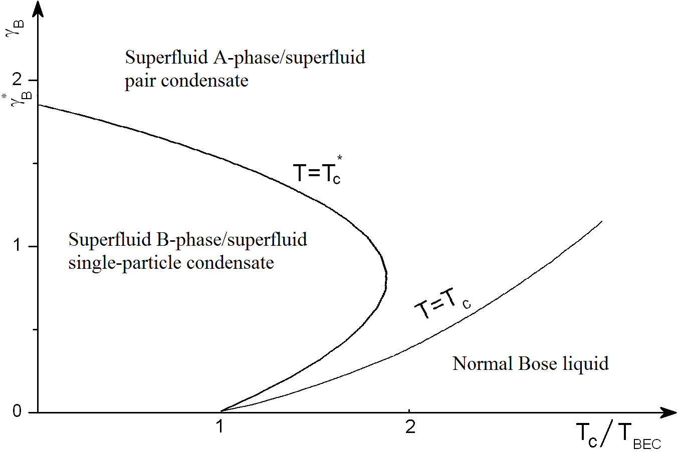
Figure 29: Phase diagram of a 3D Bose-liquid, illustrating the successive phase transitions with decreasing $T$ and $\gamma_{B}$, from normal state to the superfluid $A$-phase (superfluid pair condensate) and from the superfluid $A$-phase to the superfluid $B$-phase (superfluid single-particle condensate).

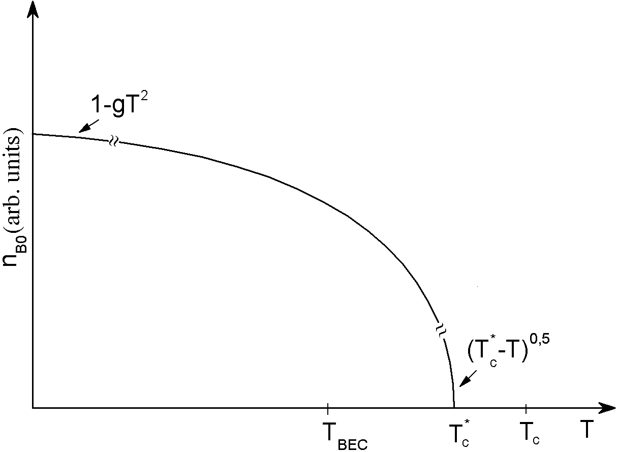
Figure 30: Temperature dependence of condensate fraction $n_{B0}$ in a superfluid 3D Bose-liquid.

As $\gamma_{B}\rightarrow 0$, $T_{c}$ approaches $T_{BEC}$, and therefore, the $T_{c}$ in the right-hand side of Eq. (165) can be replaced by $T_{BEC}$. While the expression $k_{B}T_{c}/\xi_{BA}$ in Eq. (165) may be roughly replaced by $\sqrt{2}k_{B}T_{BEC}/\xi_{BA}$ at $\gamma_{B}>0.3$. The phase diagram of a 3D Bose-liquid derived from studies of the onset temperatures ($T^{*}_{c}$ and $T_{c}$) of the single particle and pair condensations of attracting bosons is presented in Fig. 29. The temperature dependence of the fraction of condensed bosons in the $k=0$ state $n_{B0}$ is shown in Fig. 30.

VII.5 C. Two distinct superfluid states of a 2D Bose-liquid

We now turn to the case of an interacting 2D Bose system and examine the possibility of the existence of two distinct single particle and pair boson condensates and superfluid states arising in this system. We first consider the single-particle and pair condensations of attracting 2D Bosons at $T=0$. Replacing the summation in Eqs. (VII.1)-(VII.1) by an integration, we can find the critical values of $\gamma_{B}$ and $\tilde{\mu}_{B}$ at which the gap energy $\Delta_{g}$ vanishes in the excitation spectrum of a superfluid 2D Bose-liquid. Solving the integral equations and then taking into account that $\xi_{BA}>>\tilde{\mu}_{B}$ and $2\rho_{B}/D_{B}=\tilde{\mu}_{B}=2k_{B}T_{0}$, we find the critical value of $\gamma_{B}=\tilde{V}_{B}D_{B}$ from the equation

$$\gamma^{*}_{B}=\frac{1}{ln[1+\xi_{BA}/k_{B}T_{0}]},$$ (166)

where $T_{0}=2\pi\hbar^{2}\rho_{B}/m_{B}$.

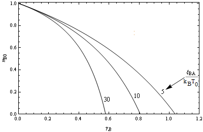
Figure 31: Dependence of the condensate fraction on the coupling constant $\gamma_{B}$ in 2D Bose superfluids at $T=0$ and $\xi_{BA}/k_{B}T_{0}$=5, 10 and 30.

The pair condensation of attracting 2D bosons occurs at $\gamma_{B}>\gamma^{*}_{B}$. While the single-particle condensation of attracting 2D bosons sets in at $\gamma_{B}\leq\gamma^{*}_{B}$ and the condensate fraction is determined from the following equations (see Appendix B):

$$2(\rho_{B}-\rho_{B0})\simeq D_{B}\tilde{\mu}_{B},$$ (167)

$$\rho_{B0}=\frac{D_{B}\tilde{\mu}_{B}}{\gamma_{B}}$$

$$\left[1-\frac{\gamma_{B}}{2}\ln\left(\frac{\sqrt{\xi^{2}_{BA}+2\tilde{\mu}_{B}\xi_{BA}}+(\xi_{BA}+\tilde{\mu}_{B})}{\tilde{\mu}_{B}}\right)\right].$$

The dependence of the condensate fraction $n_{B0}$ on the coupling constant $\gamma_{B}$ in attractive 2D Bose systems at $T=0$ is shown Fig. 31 for $\xi_{BA}/k_{B}T_{0}=$5, 10, and 30.

The ground-state energy of a 2D Bose-liquid at $\gamma_{B}\leq\gamma^{*}_{B}$ and $\tilde{\mu}_{B}=\Delta_{B}<<\xi_{BA}$ is given by

$$W_{0}\simeq\frac{1}{2}D_{B}\Delta^{2}_{B}\Omega\Big{[}1-2ln\frac{2\xi_{BA}}{\Delta_{B}}-\frac{2\Delta_{B}}{\xi_{{BA}}}\Big{]}.$$ (169)

Then the superfluid condensation energy of attracting 2D bosons at $\xi_{BA}/\Delta_{B}\simeq 5$ is defined as

$$E_{S}=W_{0}(\Delta_{B}=0)-W_{0}(\Delta_{B}>0)\simeq 2D_{B}\Delta^{2}_{B}\Omega.$$ (170)

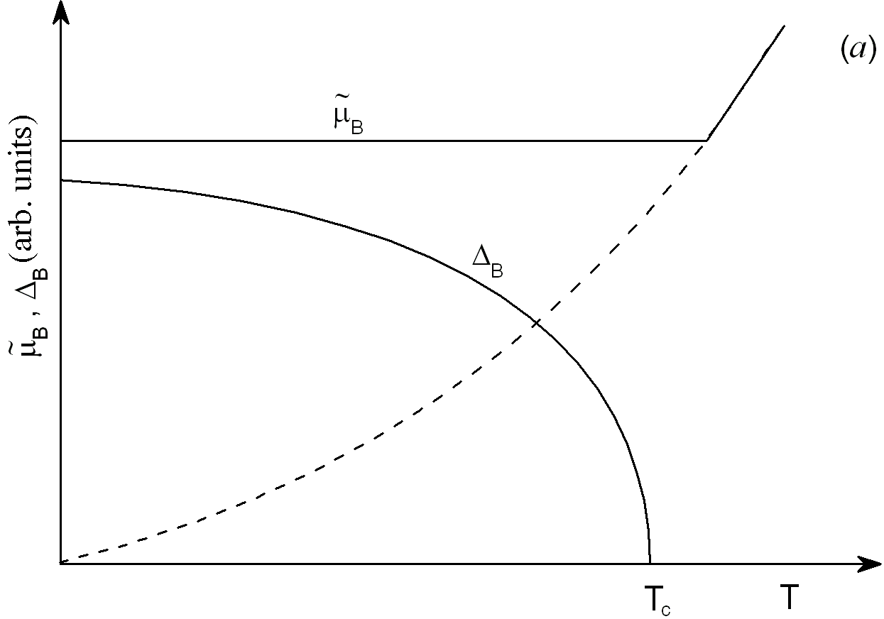
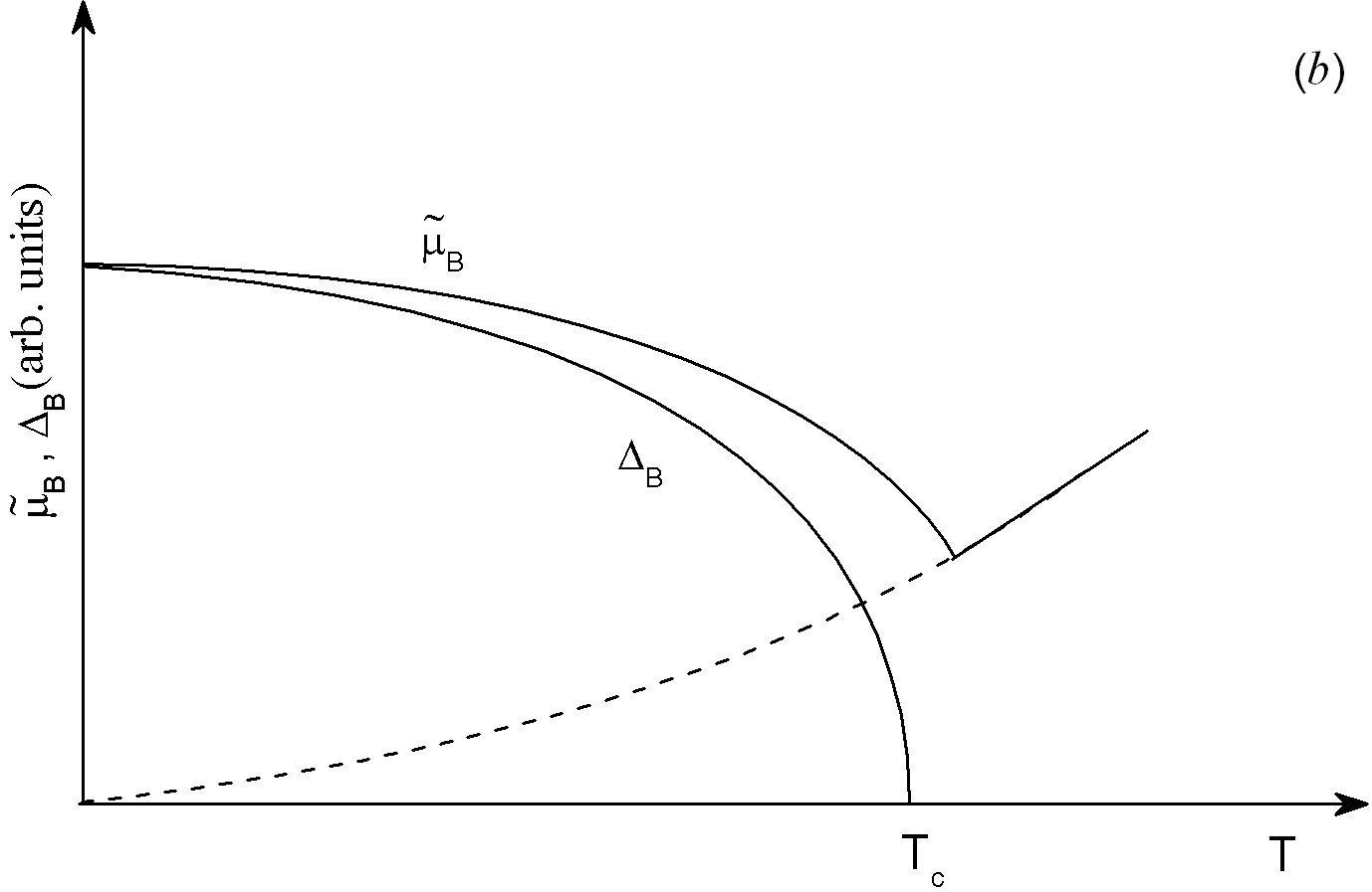
Figure 32: Temperature dependences of the chemical potential $\tilde{\mu}_{B}$ and coherence parameter $\Delta_{B}$ of a 2D Bose-liquid (solid curves), for different coupling constants $\gamma_{B}$: (a) for $\gamma_{B}>\gamma^{*}_{B}$ and (b) for $\gamma_{B}<\gamma^{*}_{B}$. Dashed curves indicate temperature dependences of the chemical potential of ideal 2D Bose gases.

We turn next to the case $T\neq 0$. In this case, the energy gap

$$\Delta_{g}=-2k_{B}T\ln\left[\frac{1}{2}\left(\sqrt{4+\zeta^{2}}-\zeta\right)\right],$$ (171)

always exists in $E_{B}(k)$, 224 , where $\zeta=\exp[(\tilde{\mu}_{B}-2k_{B}T_{0})/2k_{B}T]$. Therefore, at $T>0$ we have deal only with the superfluid pair condensation of attracting 2D bosons. At $T<<T_{c}$ the temperature dependence of the coherence parameter $\Delta_{B}$ could be approximated as (see Appendix D)

$$\Delta_{B}(T)\simeq-\frac{z}{2}k_{B}T+\sqrt{\Delta^{2}_{B}(0)+\frac{z-4}{4z}(zk_{B}T)^{2}},$$

where $z={\exp(4/\gamma_{B})}/{[1+(\exp(2/\gamma_{B})/2)^{2}]}$, $\Delta_{B}(0)\simeq({\xi_{BA}+\tilde{\mu}_{B}})/{\sqrt{1+(\exp(2/\gamma_{B})/2)^{2}}}.$

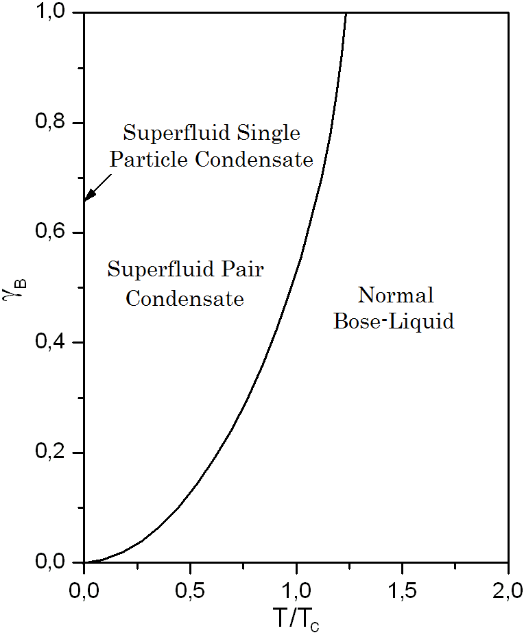
Figure 33: The phase diagram of an interacting 2D Bose gas for $\gamma_{B}\leq 1$, illustrating the possible superfluid single particle condensate (at $T=0$), superfluid pair condensate (at $T>0$) and normal (at $T>T_{c}$) states of a 2D Bose-liquid.

As seen from Eq. (VII.5), $\Delta_{B}(T)$ decreases with increasing $T$ and one can assume that $\Delta_{B}(T)$ tends to zero when $T$ approaches $T_{c}$. Approximate solutions of Eqs. (VII.1)-(VII.1) near $T_{c}$ lead to the following equations for determination of the temperature dependence of $\Delta_{B}$ and $\tilde{\mu}_{B}$ near $T_{c}$ (see Appendix D)

$$\Delta_{B}(T)=(2+\gamma_{B})k_{B}T_{c}\left[\left(\frac{T}{T_{c}}\right)^{2-q}-\frac{T}{T_{c}}\right],$$ (173)

and

$$\tilde{\mu}_{B}(T)=\sqrt{\Delta^{2}_{B}(T)+(2k_{B}T_{c})^{2}\left(\frac{\gamma_{B}}{2+\gamma_{B}}\right)^{2}\left(\frac{T}{T_{c}}\right)^{2q}}.$$

where the value of $q$ must be determined for the given values of $\gamma_{B}$ and $T/T_{c}$ by means of the self-consistent solution of Eq. (171), Eq. (173) and Eq. (VII.5). The temperature dependences of $\Delta_{B}$ and $\tilde{\mu}_{B}$ are shown in Figs. 32a and 32b.

It is important to go beyond the weak coupling limit and to derive a simple and more general expression for $T_{c}$, which should be valid not only for $\gamma_{B}<<1$ but also for $\gamma_{B}\lesssim 1$. Such an expression for $T_{c}$ can now be derived by equating the chemical potential of an ideal 2D Bose gas

$$\tilde{\mu}_{B}(T_{c})=k_{B}T_{c}\ln\left[1-\exp\left(-\frac{T_{0}}{T_{c}}\right)\right],$$ (175)

with the expression (VII.5) at $T=T_{c}$ (see dashed and solid curves in Figs. 32a and 32b). In so doing, we find the following expression for $T_{c}$:

$$T_{c}=-\frac{T_{0}}{\ln[1-\exp(-2\gamma_{B}/(2+\gamma_{B}))]},$$ (176)

from which at a particular case $\gamma_{B}<<1$ follows the result for $T_{c}$ presented in Ref. 224 . The phase diagram of a 2D Bose-liquid is presented in Fig. 33.

VII.6 D. Effects of mass renormalization on $T_{BEC}$ and $T_{0}$ in a Bose-liquid

In 3D and 2D Bose liquids the interaction between Bose particles may change significantly the characteristic temperatures $T_{BEC}$ and $T_{0}$ entering the expressions for $T_{c}$ and $T^{*}_{c}$. In particular, the actual BEC temperature $T_{BEC}$ in a nonideal Bose gas is turned out to be less than that in an ideal Bose gas 210 , since the renormalized mass of bosons enters the expression for $T_{BEC}$. It is essential for any theory of the Bose superfluid to account properly for the already existent effects of mass renormalization below $T_{c}$, which are caused by the effective interboson interactions. Therefore, we need to examine the effects of mass renormalization on $T_{BEC}$ and $T_{0}$.

We consider first the question of the effects of mass renormalization in 3D Bose-liquid. We will indicate how the desired expression for $\tilde{\varepsilon}_{B}(k)$ can be obtained using the effective mass approximation proposed in Ref. 210 . According to Luban 210 , the Fourier transform of the interparticle potential $V_{B}(r)$ is given by

$$V_{B}(k)=\frac{4\pi WR^{3}}{kR}\int\limits_{0}^{\infty}dxx\Phi(x)\sin kRx,$$ (177)

where $W$ and $R$ are the energy and range parameters, respectively, $x=r/R$. After expanding the $V_{B}(k)$ in a Taylor series around $kR=0$ (with a radius of convergence not smaller than $kR=1$ for $\Phi(x)=e^{-x}/x$) and some algebraic transformations 210 , one obtains

$$\tilde{\varepsilon}_{B}(k)=\tilde{\varepsilon}_{B}(0)+\frac{\hbar^{2}k^{2}}{2m_{B}^{*}},\qquad 0\leq k\leq k_{A}$$ (178)

where $k_{A}=\sqrt{2m_{B}\xi_{BA}}/\hbar\simeq(10R)^{-1}$ and $m_{B}^{*}$ satisfies

$$\frac{1}{m_{B}^{*}}=\frac{1}{m_{B}}-$$

$$\frac{V_{B}(0)}{\pi^{2}\hbar^{2}k^{2}_{R}}\int\limits_{0}^{k_{A}}dkk^{2}\frac{1}{\exp[(\tilde{\varepsilon}_{B}(0)+\hbar^{2}k^{2}/2m_{B}^{*})/T]-1},$$

where $k_{R}=\sqrt{2m_{B}\xi_{BR}}/\hbar$. Further, the density of Bose particles can be defined as

$$\rho_{B}=\frac{1}{2\pi^{2}}\int\limits_{0}^{k_{A}}dkk^{2}\frac{1}{\exp[(\tilde{\varepsilon}_{B}(0)+\hbar^{2}k^{2}/2m_{B}^{*})/T]-1}.$$

Comparing Eq. (VII.6) with Eq. (VII.6), we conclude that the effective mass of interacting bosons is

$$m_{B}^{*}=m_{B}\left[1-\frac{\rho_{B}V_{B}(0)}{\xi_{BR}}\right]^{-1}.$$ (181)

Then, the BEC temperature of bosons in a 3D Bose-liquid is defined as (see also Ref. 210 )

$$T_{BEC}^{*}(\rho_{B})=T_{BEC}(\rho_{B})\left[1-\frac{\rho_{B}V_{B}(0)}{\xi_{BR}}\right].$$ (182)

Accordingly, the BEC temperature $T_{BEC}(\rho_{B})$ of free bosons entering the expression (165) for $T_{c}$ should be replaced by $T_{BEC}^{*}(\rho_{B})$. Therefore, the behavior of $T_{c}(\rho_{B})$ is now controlled by the behavior of $T_{BEC}^{*}(\rho_{B})$. In this case, one can expect that $T_{c}$ first rises nearly as $\sim\rho_{B}^{2/3}$, and then goes through a maximum (at some $\rho_{B}=\rho_{B}^{*}$ determined from $\partial T_{BEC}^{*}(\rho_{B})/\partial\rho_{B}=0$), after that starts to decrease (Fig. 34). The description of the subsequent decreasing trend of $T_{c}$ within the present model is impossible.

A similar result can be obtained for the renormalized temperature $T_{0}^{*}(\rho_{B})$ in a 2D Bose-liquid. In this case, the Fourier transform of $V_{B}(r)$ is given by

$$V_{B}(k)=2\pi\int\limits_{0}^{\infty}drrV_{B}(r)J_{0}(kr),$$ (183)

where $J_{0}(kr)$ is the zero-order Bessel function.

Further, the potential $V_{B}(r)$ may be approximated just like in the case of a 3D Bose-liquid as $V_{B}(r)=W\Phi(x)$. Then we have

$$V_{B}(k)=2\pi WR^{2}\int\limits_{0}^{\infty}dxx\Phi(x)J_{0}(kRx).$$ (184)

After expanding $J_{0}(kRx)$ in a Taylor series around $kR=0$ (with a radius of convergence not smaller than $kR=2$ for $\Phi(x)=e^{-x}/x$) and some algebraic transformations (see Appendix E), we obtain the equations, which are similar to Eqs. (178) - (181). The characteristic temperature $T_{0}^{*}(\rho_{B})$ in a 2D Bose-liquid is defined as

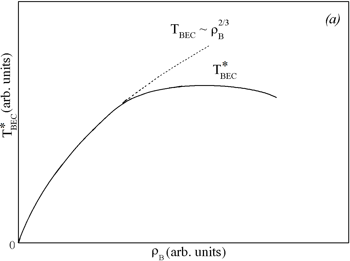
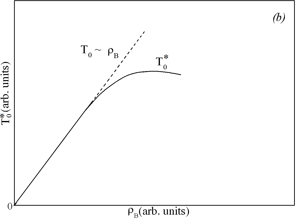
Figure 34: The dependence of $T_{BEC}^{*}$ on $\rho_{B}$ in a 3D Bose-liquid.(b) The dependence of $T_{0}^{*}$ on $\rho_{B}$ in a 2D Bose-liquid. The quantities $T_{BEC}$ and $T_{0}$ are the corresponding quantities for the 3D and 2D ideal Bose gases.

$$T_{0}^{*}(\rho_{B})=T_{0}(\rho_{B})\left[1-\frac{\rho_{B}V_{B}(0)}{\xi_{BR}}\right].$$ (185)

The characteristic temperature $T_{0}$ entering the expression (176) should be replaced by $T_{0}^{*}$. From Eq. (185) it follows that at $\rho_{B}=\rho_{B}^{*}=\xi_{BR}/2V_{B}(0)$, $\partial T_{c}/\partial\rho_{B}=0$ and $\partial^{2}T_{c}/\partial\rho^{2}_{B}<0$. This means that $T_{c}$ first increases nearly as $\sim\rho_{B}$ and then goes through a maximum at $\rho_{B}=\rho_{B}^{*}$, after that will decrease just as in the case of a 3D Bose-liquid.

VII.7 F. Specific heat of a superfluid Bose-liquid

The specific heat of a superfluid Bose-liquid is determined from the relation 22 ; 22

$$C_{v}(T)=\frac{1}{k_{B}T^{2}}\sum_{k}n_{B}(k)[1+n_{B}(k)]\Big{\{}E_{B}^{2}(k)-$$

$$-T\left[\varepsilon\frac{\partial\tilde{\mu}_{B}}{\partial T}+\frac{1}{2}\frac{\partial}{\partial T}\Delta^{2}_{g}\right]\Big{\}}.$$ (186)

At low temperatures, we can assume $k_{B}T<<\tilde{\mu}_{B}$, $\Delta_{B}$ and $\Delta_{B}\approx const$, $\tilde{\mu}_{B}\approx const$. Therefore, the specific heat of a 3D superfluid Bose-liquid is given by

$$C_{v}(T)\simeq\frac{\Omega D_{B}k_{B}}{4(k_{B}T)^{2}}\int\limits_{0}^{\infty}\sqrt{\varepsilon}\frac{d\varepsilon}{\sinh^{2}[E_{B}(\varepsilon)/2k_{B}T]}E^{2}_{B}(\varepsilon).$$

At $\gamma_{B}>\gamma^{*}_{B}$ and $\Delta_{g}>2k_{B}T$ the function $\sinh[E_{B}(\varepsilon)/2k_{B}T]$ under the integral in Eq. (VII.7) can be replaced by $(1/2)\exp[E_{B}(\varepsilon)/2k_{B}T]$. Further, taking into account that the main contribution to the integral in Eq. (VII.7) comes from the small values of $\varepsilon<<\Delta_{g}$, we can replace $E_{B}(\varepsilon)$ by $\sqrt{2\tilde{\mu}_{B}\varepsilon+\Delta^{2}_{g}}$ and use the Taylor expansion in the exponent $\sqrt{2\tilde{\mu}_{B}\varepsilon+\Delta_{g}^{2}}\approx\Delta_{g}+\tilde{\mu}_{B}\varepsilon/\Delta_{g}$. Then evaluating the integral in Eq. (VII.7), we get

$$C_{v}(T)\simeq\frac{3\Omega D_{B}\Delta_{g}^{5/2}k_{B}}{2\tilde{\mu}_{B}^{3/2}}\sqrt{\pi k_{B}T}\times$$

$$\times\left[1+\frac{1}{3}\sqrt{\frac{2}{\pi}}\frac{\Delta_{g}}{k_{B}T}\right]\exp\left(-\frac{\Delta_{g}}{k_{B}T}\right).$$ (188)

However, for $\gamma_{B}<\gamma_{B}^{*}$ and $T<T^{*}_{c}$ the excitation spectrum of a 3D superfluid Bose-liquid at small values of $k$ is phonon-like $E_{B}(k)\simeq\sqrt{2\tilde{\mu}_{B}\varepsilon}=\sqrt{\tilde{\mu}_{B}/m_{B}}\hbar k$. Then Eq. (VII.7) after the substitution $E_{B}(\varepsilon)/2k_{B}T=x$ takes the form

$$C_{v}(T)\simeq\frac{4\sqrt{2}\Omega D_{B}k_{B}(k_{B}T)^{3}}{\tilde{\mu}_{B}^{3/2}}\int\limits_{0}^{\infty}\frac{x^{4}dx}{sinh^{2}x}=$$

$$\frac{\Omega D_{B}k_{B}(k_{B}T)^{3}}{\tilde{\mu}_{B}^{3/2}}\Big{(}\frac{2\sqrt{2}\pi^{4}}{15}\Big{)},$$ (189)

where the value of the integral is equal to $(2)^{-3}\Gamma(5)\zeta(4)=\pi^{4}/30$ (see, e.g., Ref. 126 ).

As appears from the above, the phonon-like $T^{3}$ dependence of $C_{v}(T)$ is expected at $T<T^{*}<<T_{c}$, as it was observed in superfluid ⁴He below 1 K 214 . According to the expressions (157) and (158), the temperature derivaties of $\tilde{\mu}_{B}(T)$ and $\Delta_{B}(T)$ would vary rapidly and diverge as $(T_{c}-T)^{-1/2}$ near $T_{c}$. Therefore, the main contribution to $C_{v}(T)$ at temperatures close to $T_{c}$ comes from the second term of Eq. (VII.7) and the specific heat of a 3D Bose-liquid varies rapidly as $C_{v}(T)\sim const/(T_{c}-T)^{1/2}$ near $T_{c}$. More importantly, this behavior of $C_{v}(T)$ at $T\rightarrow T_{c}$ is similar to that of the specific heat of superfluid ⁴He at $T_{\lambda}$. Similarly, as $T$ approaches $T^{*}_{c}$ from below the specific heat of the Bose superfluid varies now as $C_{v}(T)\sim const/(T^{*}_{c}-T)^{1/2}$ according to Eqs. (159) and (VII.7). Such a rapid temperature dependence of $C_{v}(T)$ eventually leads also to a $\lambda$-like anomaly at $T^{*}_{c}$. The above predicted behaviors of $C_{v}(T)$ near $T_{c}^{*}$ and $T_{c}$ are shown in Fig. 35. Clearly, $C_{v}(T)$ is proportional to $T^{3/2}$ above $T_{c}$.

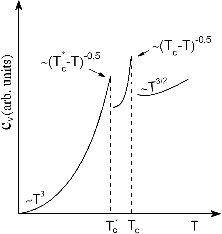
Figure 35: Temperature dependence of the specific heat of a 3D superfluid Bose-liquid showing the existence of two distinct $\lambda$-like anomalies in $C_{v}(T)$ at $\gamma_{B}<<\gamma_{B}^{*}$ .

The specific heat of a 2D superfluid Bose-liquid at low temperatures can be determined in the same manner using the above-mentioned approximations. Then, evaluating the integral in Eq. (VII.7) at $\Delta_{g}>2k_{B}T$, we find

$$C_{v}(T)\simeq\frac{2\Omega D_{B}k_{B}\Delta^{2}_{g}}{\tilde{\mu}_{B}}\left[1+\frac{\Delta_{g}}{2k_{B}T}\right]\exp\left(-\frac{\Delta_{g}}{k_{B}T}\right).$$

Further, for $\Delta_{g}<2k_{B}T$ we obtain from Eq. (VII.7) (see Appendix D)

$$C_{v}(T)\simeq 76\Omega D_{B}k_{B}\Big{(}\frac{k_{B}T}{\Delta_{B}}\Big{)}^{2}.$$ (191)

In this case the temperature dependence of $C_{v}(T)$ in a 2D superfluid Bose-liquid is also very close to phonon-like one.

VII.8 G. Stability of attractive Bose systems

For attractive Bose systems, the problem of their stability relative to spontaneous collapse can arise in the study of the superfluid states in such Bose systems. To escape a collapse in a 2D attractive Bose gas of holons, the strong Hartree-Fock repulsion, which ensures a positive compressibility, has been introduced in Ref. 224 . Here, we briefly discuss the stability of the superfluid states in 3D and 2D attractive Bose systems.

In the weak coupling limit ($\gamma_{B}<<1$), the single particle condensation in a 3D attractive Bose gas with $\rho_{B}\sim\rho_{B0}$ is expected in a wide temperature range from $T=0$ to $T^{*}_{c}<T_{c}$. In this limiting case, one obtains $\Delta_{B}\simeq\rho_{B}\tilde{V}_{B}$ 226 and $\tilde{\mu}_{B}\simeq 2\rho_{B}(V_{BR}-\frac{3}{2}V_{BA})$, so that the compressibility just like in the case of a 2D attractive Bose gas of holons 224 is given by

$$K_{B}=\rho^{2}_{B}\frac{\partial\tilde{\mu}_{B}}{\partial\rho_{B}}\simeq 2\rho_{B}^{2}\left(V_{BR}-\frac{3}{2}V_{BA}\right),$$ (192)

which is essentially positive at $V_{BR}>1.5V_{BA}$. This means that the 3D Bose gas with the attractive and repulsive interboson interactions is stable.

In the strong coupling limit ($\gamma_{B}>\gamma_{B}^{*}$ or $\tilde{\mu}_{B}>\Delta_{B}$), we deal with the pair condensation of bosons in attractive Bose systems. Especially, for $\gamma_{B}>>\gamma_{B}^{*}$ the behavior of such Bose systems seems to be very close to a dilute gas limit. In this case, the quantities $\tilde{\mu}_{B}$ and $K_{B}$ for 3D and 2D Bose systems are determined from the relations $\tilde{\mu}_{B}=2\rho_{B}(V_{BR}-V_{BA})-\frac{E_{b}}{2}$ (where $E_{b}=2\tilde{\mu_{B}}$ is the binding energy of a boson pair in a dilute Bose gas 220 ) and $K_{B}=2\rho_{B}^{2}(V_{BR}-V_{BA})$. It follows that in the strong coupling limit the 3D and 2D attractive Bose systems are stable at $V_{BR}>V_{BA}$. One can see that in the strong coupling limit the pair condensation of attracting bosons leads to the formation of $N_{B}/2$ boson molecules. Note that the fermion pairs (molecules) are also formed in attractive Fermi systems in the dilute limit 38 ; 227 .

Thus, the 3D and 2D attractive Bose systems undergoing the single particle and pair condensations are stable for $V_{BR}>>V_{BA}$ (when $\gamma_{B}<<\gamma^{*}_{B}$) and for $V_{BR}>V_{BA}$ (when $\gamma_{B}>\gamma^{*}_{B}$).

VIII VIII. Novel Bose-liquid superconductivity and superfluidity in high-$T_{c}$ cuprates and other systems

In this section, we convincingly prove that the underlying mechanisms of unconventional superconductivity and superfluidity observed in various substances are fundamentally different from the BCS condensation of fermionic Cooper pairs and the so-called $s$-, $p$- or $d$-wave BCS-type superconductivity (superfluidity). Actually, the superconducting/superfluid transition in high-$T_{c}$ cuprates 33 and other unconventional superconductors 30 and superfluid ³He 198 closely resembles the $\lambda$-like superfluid transition in liquid ⁴He. In particular, various experiments 26 ; 28 ; 33 ; 35 ; 60 strongly suggest that the underdoped, optimally doped and moderately overdoped cuprates should not be BCS-type superconductors. Therefore, it is necessary to go beyond the framework of both the BCS condensation model and the BEC model for understanding the phenomena of unconventional superconductivity and superfluidity in high-$T_{c}$ cuprates and other intricate systems. Here, we encounter a novel superconducting/superfluid state of matter, which is a superfluid Bose liquid of bosonic Cooper pairs, and we have deal with low-density bosonic matter exhibiting novel superconductivity (superfluidity) below $T_{c}$ and a $\lambda$-like superconducting/superfluid transition at $T_{c}$, similar to the $\lambda$-transition in liquid ⁴He.

We now present a radically new microscopic theory of unconventional superconductivity and superfluidity in high-$T_{c}$ cuprates and other systems based on the above theory of Bose superfluids, which describes the genuine superconducting/superfluid states arising at the pair and single particle condensations of attracting bosons (Cooper pairs and ⁴He atoms). We demonstrate that only a small attractive part of a Bose gas in these systems can undergo a superfluid phase transition at $T_{c}$ and the mean field theory of 3D and 2D Bose superfluids is well consistent with existing experimental data and make experimentally testable predictions of the distinctive features of bosonic order parameter $\Delta_{B}$, novel superconducting/superfluid states and properties of various high-$T_{c}$ cuprates and other related systems.

VIII.1 A. Novel superconducting states and properties of high-$T_{c}$ cuprates and their experimental manifestations

The high-$T_{c}$ cuprate superconductivity is still invariably considered as the Fermi-liquid superconductivity based on the BCS-type ($s$- or $d$- wave) pairing of electrons and holes. In order to understand this phenomenon, we take an alternative view that the genuine superconductivity in high-$T_{c}$ cuprates results from the superfluid condensation of the attractive Bose gases of polaronic Cooper pairs with low densities ($\rho_{B}<<n_{c}$). Such composite bosons repel one another at small distances between them and their net interaction is attractive at large distances. In high-$T_{c}$ cuprates, attractive interactions between bosonic Cooper pairs result from their polaronic carriers interacting with lattice vibrations. The energy of such an attractive interaction between bosonic Cooper pairs would be of the order of $\hbar\omega_{0}$ (i.e. $\xi_{BA}\sim\hbar\omega_{0}$). The 3D mean-field equations for determining the coherence (i.e., superconducting order) parameter $\Delta_{SC}=\Delta_{B}$ and the condensation temperature $T_{c}$ of such bosonic Cooper pairs can be written as (see Appendix B):

$$\frac{2}{D_{B}\tilde{V}_{B}}=\int^{\xi_{BA}}_{0}\sqrt{\varepsilon}\frac{\coth\left[\frac{\sqrt{(\varepsilon+\tilde{\mu}_{B})^{2}-\Delta^{2}_{B}}}{2k_{B}T}\right]}{\sqrt{(\varepsilon+\tilde{\mu}_{B})^{2}-\Delta^{2}_{B}}}d\varepsilon,$$ (193)

$$\frac{2\rho_{B}}{D_{B}} = \int^{\infty}_{0}\sqrt{\varepsilon}\Bigg{\{}\frac{\varepsilon+\tilde{\mu}_{B}}{\sqrt{(\varepsilon+\tilde{\mu}_{B})^{2}-\Delta^{2}_{B}}}\times$$ (194)

$$\times\coth\left[\frac{\sqrt{(\varepsilon+\tilde{\mu}_{B})^{2}-\Delta^{2}_{B}}}{2k_{B}T}\right]-1\Bigg{\}}d\varepsilon.$$

Solutions of Eqs. (193) and (194) allow us to examine closely the novel superconducting/superfluid states arising in high-$T_{c}$ cuprates. In the strong coupling limit ($\gamma_{B}>\gamma^{*}_{B}$) the excitation spectrum of a 3D Bose superfluid $E_{B}(k)$ has the energy gap $\Delta_{g}=\sqrt{\tilde{\mu}_{B}^{2}-\Delta^{2}_{B}}$ in the temperature range $0\leqslant T<T_{c}$ (see Fig. 27a). However, in the intermediate and weak coupling regimes, the boson excitation spectrum $E_{B}(k)$ becomes gapless at $T\leq T^{*}_{c}<<T_{c}$ (for $1<\gamma_{B}<\gamma_{B}^{*}$) or at $T\leq T^{*}_{c}<T_{c}$ (for $\gamma_{B}<<1$). For $\gamma_{B}<\gamma^{*}_{B}$ and $\Delta_{g}=0$, Eqs. (193) and (194) become (see Appendix B)

$$\frac{2}{D_{B}\tilde{V}_{B}}=\frac{2\rho_{B0}}{D_{B}\tilde{\mu}_{B}}+\int^{\varepsilon_{BA}}_{0}\sqrt{\varepsilon}\frac{\coth\left[\frac{\sqrt{\varepsilon^{2}+2\tilde{\mu}_{B}\varepsilon}}{2k_{B}T}\right]}{\sqrt{\varepsilon^{2}+2\tilde{\mu}_{B}\varepsilon}}d\varepsilon,$$

$$\frac{2\rho_{B}}{D_{B}} = \frac{2\rho_{B0}}{D_{B}}+\int^{\infty}_{0}\sqrt{\varepsilon}\Bigg{\{}\frac{\varepsilon+\tilde{\mu}_{B}}{\sqrt{\varepsilon^{2}+2\tilde{\mu}_{B}\varepsilon}}\times$$ (196)

$$\times\coth\left[\frac{\sqrt{\varepsilon^{2}+2\tilde{\mu}_{B}\varepsilon}}{2k_{B}T}\right]-1\Bigg{\}}d\varepsilon,$$

where $\rho_{B0}$ is the density of bosonic Cooper pairs with $k=0$ and $\varepsilon=0$.

The self-consistent equations (193)-(196) can be solved both namerically and analytically (see Sec. VII). These equations have collective solutions for the attractive interboson interaction $\tilde{V}_{B}$. The superfluid state is characterized by the coherence parameter $\Delta_{B}$ which vanishes at $T=T_{c}$, that marks the vanishing of a macroscopic superfluid condensate of bosonic Cooper pairs. For $T\leq T_{c}^{*}$, the gapless and linear (at small $k$), phonon-like spectrum $E_{B}(k)$ in the superconducting state is similar to the excitation spectrum in superfluid ⁴He and satisfies also the criterion for superfluidity, i.e., the critical velocity of Cooper pairs $v_{c}=\hbar^{-1}{(\partial E_{B}(k)/\partial{k})}_{min}>0$ satisfies the condition for the existence of their superfluidity. By solving Eqs. (193) and (194) for $\Delta_{g}>0$ ($T>T^{*}_{c}$) and then Eqs. (VIII.1) and (196) for $\Delta_{g}=0$ $(T\leq T^{*}_{c})$, we find that the pair condensation of bosons at $T>T^{*}_{c}$ will correspond to a smaller value of both the chemical potential $\tilde{\mu}_{B}$ and the order parameter $\Delta_{B}<\tilde{\mu}_{B}$, while their single particle condensation at $T\leq T^{*}_{c}$ will correspond to a much larger value of the chemical potential $\tilde{\mu}_{B}=\Delta_{B}$. The self-consistent solutions of Eqs. (193)-(196) allow us to establish the following universal law of superfluid condensation of bosonic Cooper pairs in non-BCS-type superconductors: the pair condensation of attracting Bose particles occurs first at $T_{c}$ and then their single particle condensation sets in at a lower temperature $T_{c}^{*}$ than the $T_{c}$. According to this law, upon lowering the temperature, a $\lambda$-like superconducting phase transition occurs at $T_{c}$ (see Fig. 35) and a new first-order phase transition in the superconducting state occurs then at $T\leq T^{*}_{c}$. The validity of the above law describing the occurrence of a $\lambda$-like phase transition at $T_{c}$ and a first-order phase transition somewhat below $T_{c}$ or even far below $T_{c}$ has been experimentally confirmed in high-$T_{c}$ cuprates 33 ; 229 ; 230 ; 231 and other systems (see below).

Thus, single particle and pair condensates of bosonic Cooper pairs are two distinct superconducting phases in high-$T_{c}$ cuprates just like A and B phases in superfluid ³He. The occurrence of the Bose-liquid superconductivity in these systems is characterized by a non-zero coherence parameter $\Delta_{B}$ which defines the bond strength of all condensed bosonic Cooper pairs - boson superfluid stiffness. Therefore, excitations of a superfluid Bose condensate of Cooper pairs in high-$T_{c}$ cuprates are collective excitations of many particles (all bosons participate in the excitation). Such excitations should not be measured by single-particle spectroscopies, as noted also in Ref. 228 . The new excitation-energy scale of a superfluid Bose condensate of Cooper pairs in cuprate superconductors will be related to the coherence parameter $\Delta_{B}$ and to $T_{c}$. The frictionless flow of a Bose-liquid of Cooper pairs would be possible under the condition $\Delta_{B}>0$. While the BCS-like fermionic excitation gap $\Delta_{F}$ characterizing the bond strength of Cooper pairs exists above $T_{c}$ as the pseudogap 21 ; 22 ; 33 ; 34 ; 35 , which is also necessary ingredient for unconventional superconductivity and superfluidity of bosonic Cooper pairs.

The high-$T_{c}$ cuprates are fundamentally different from the BCS-type superconductors. In conventional metals and heavily overdoped cuprates with large Fermi energies, the superconducting state is characterized only by the BCS-like (fermionic) order parameter $\Delta_{F}$ appearing at $T_{c}$ and the onset temperature of Cooper pairing $T^{*}$ coincides with $T_{c}$. In contrast, for high-$T_{c}$ cuprates with small Fermi energies, the emergence of unconventional superconductivity is a two-stage process 21 : the formation of bosonic (polaronic) Cooper pairs at $T^{*}>T_{c}$ and the subsequent condensation of such Cooper pairs into a superfluid Bose-liquid state at $T_{c}$. In these high-$T_{c}$ materials, the superconducting state is characterized by the bosonic order parameter $\Delta_{B}$ appearing at $T_{c}$, since the onset temperature $T^{*}$ of unconventional Cooper pairing is different from the superconducting transition temperature $T_{c}$ (Fig. 36), as observed in many experiments 7 ; 26 ; 33 .

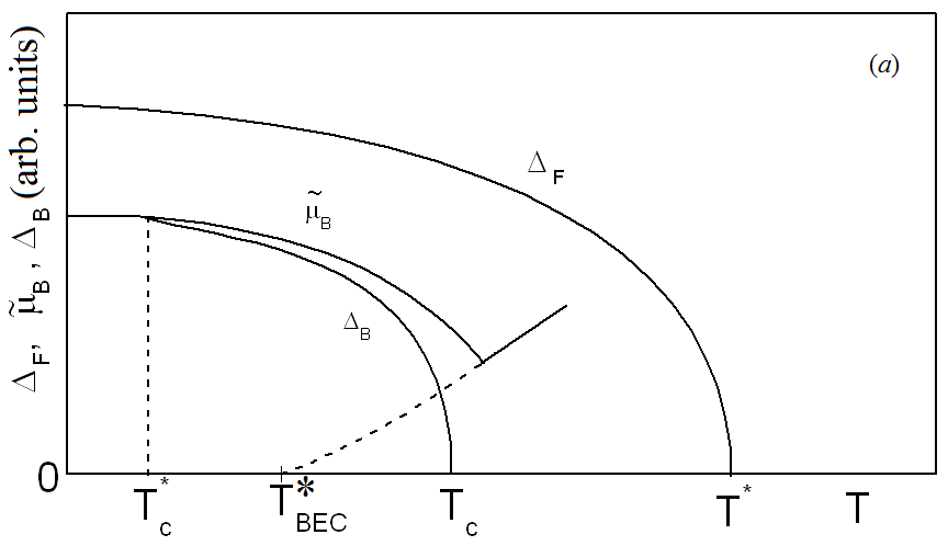
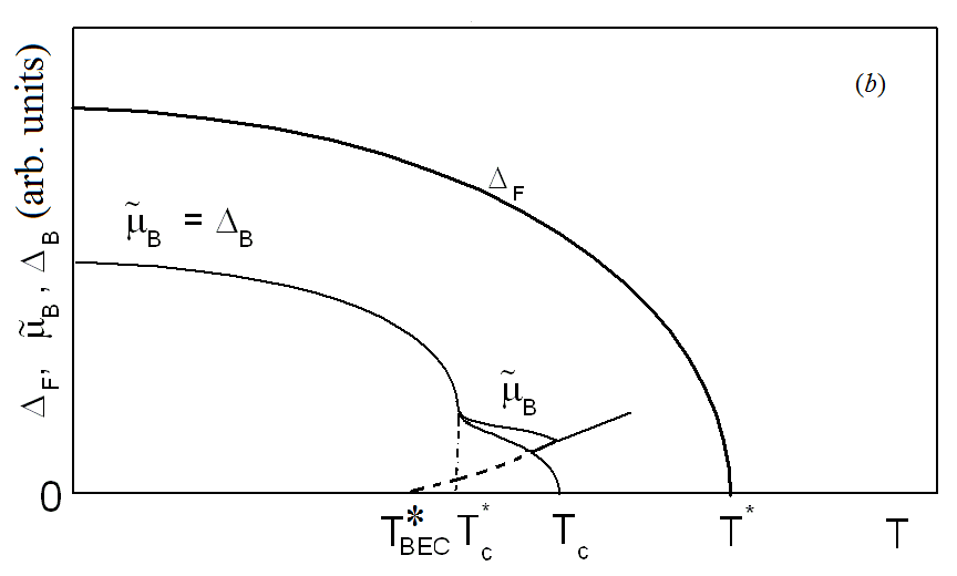
Figure 36: (a) Temperature dependences of the BCS-like pseudogap $\Delta_{F}$ appearing at a temperature $T^{*}$ above $T_{c}$ and the superconducting order parameter $\Delta_{SC}=\Delta_{B}$ in 3D non-BCS (bosonic) superconductors at $\gamma_{B}<\gamma_{B}^{*}$, where $\tilde{\mu}_{B}$ is the chemical potential of an attracting Bose gas of Cooper pairs, $T^{*}_{BEC}$ is the renormalized BEC temperature, $T_{c}$ and $T^{*}_{c}$ are the onset temperatures of the second-order and first-order phase transitions to the superconducting state. (b) Temperature dependences of $\Delta_{F}$ and $\Delta_{SC}$ in 3D bosonic superconductors at $\gamma_{B}<<\gamma^{*}_{B}$.

The novel Bose-liquid superconductivity would occur in underdoped, optimally doped and moderately overdoped cuprates under the coexistence of two fundamentally different fermionic and bosonic order parameters. In these unconventional superconductors (Fig. 36$a$ and 36$b$), the disappearance of the coherence parameter $\Delta_{B}$ or superfluid condensate of bosonic Cooper pairs at $T=T_{c}$ is not accompanied yet by the destruction of such Cooper pairs which disappear at higher temperatures (i.e. at $T=T^{*}>T_{c}$ or even at $T=T^{*}>>T_{c}$). Thus, the situation is completely different in high-$T_{c}$ cuprates in which the superconducting order parameter $\Delta_{B}(=\Delta_{SC})$ appearing at $T_{c}$ and the BCS-like gap opening at the Fermi surface above $T_{c}$ have different origins. For reasons given above, most of experimental techniques capable of measuring the BCS-like fermionic excitation gap $\Delta_{F}$ 43 are turned out to be incapable of identifying the genuine (bosonic) superconducting order parameter $\Delta_{B}$ in the cuprates, from underdoped to overdoped regime (see also Ref. 228 ). There is still confusion in the literature concerning the superconducting order parameter in high-$T_{c}$ cuprates, since it is often identified as a BCS-like ($s$- or $d$-wave) gap on the basis of tunneling and ARPES data. Actually, the single particle tunneling spectroscopy and ARPES provide only information about the excitation gaps $\Delta_{p}$ and $\Delta_{F}$ at the Fermi surface but they fail to measure the energy of the collective excitation of all condensed bosonic Cooper pairs and to identify the genuine superconducting order parameter $\Delta_{B}$ appearing below $T_{c}$ in unconventional cuprate superconductors. The distinctive features of the novel superconducting states and properties of high-$T_{c}$ cuprates and their experimental manifestations will be discussed below.

VIII.2 1. Kink-like behavior of the bosonic superconducting order parameter near $T^{*}_{c}<T_{c}$

The numerical and analytical solutions of the self-consistent equations (193)-(196) allow us to predict the possible behaviors of $\Delta_{B}(T)$ as a function of temperature and $\gamma_{B}$. For $\gamma_{B}<\gamma_{B}^{*}$, we can define a characteristic temperature $T_{c}^{*}$ to be that temperature at which $\Delta_{B}(T)$ begins to drop suddenly from its low-temperature value and the energy gap $\Delta_{g}(T)$ begins to appear in $E_{B}(k)$ above $T_{c}^{*}$. In the temperature range $0\leq T<T_{c}^{*}$, the coherence parameter $\Delta_{B}$ shows very weak $T$ dependence. But the value of $\Delta_{B}$ changes rapidly near $T_{c}^{*}$. On the other hand, $\Delta_{B}$ rapidly increases as $T$ approaches $T_{c}^{*}$ from above and the first-order phase transition in the superconducting state occur at $T=T_{c}^{*}$. As a consequence, the self-consistent equations (193)-(196) for the temperature dependent coherence parameter $\Delta_{B}(T)$ suggest that there is a crossever temperature $T_{c}^{*}$ of interest at $\gamma_{B}<\gamma_{B}^{*}$ below $T_{c}$. As mentioned in Sec. VII, in the vicinity of $T_{c}^{*}$ the coherence parameter $\Delta_{B}$ begins to acquire a strong temperature dependence (see Eq. (159)). At $T\sim T_{c}^{*}$ the bosonic order parameter $\Delta_{B}$ rapidly increases as $T$ approaches $T_{c}^{*}$ from above. Therefore, the temperature dependence of the bosonic superconducting order parameter $\Delta_{SC}=\Delta_{B}$ in high-$T_{c}$ cuprates is unusual and has a kink-like feature near the characteristic temperature $T^{*}_{c}$ which will be somewhat lower than $T_{c}$ or even will be much lower than $T_{c}$. This kink-like feature in $\Delta_{SC}(T)$ is less pronounced for $\gamma_{B}<\gamma_{B}^{*}$ and $T_{c}^{*}<<T_{c}$, but it is more pronounced for $\gamma_{B}<<\gamma_{B}^{*}$ (i.e. somewhat below $T_{c}$). Such a kink-like behavior of $\Delta_{SC}(T)$ near $T^{*}_{c}$ in turn leads to the radical changes of other superconducting parameters (e.g., critical magnetic fields and current, etc.) of high-$T_{c}$ cuprates. Some experiments 232 indicate that the superconducting order parameter $\Delta_{SC}(T)$ in the cuprates has a kink-like feature near the characteristic temperature $T^{*}_{c}$ ($\lesssim 0.6T_{c}$). We believe that the kink-like behavior of the bosonic superconducting order parameter $\Delta_{SC}(=\Delta_{B})$ seems to be quite plausible for high-$T_{c}$ cuprates. Indeed, the temperature dependence of $\Delta_{SC}(T)$ observed in the ceramic high-$T_{c}$ superconductor $\rm{EuBa_{2}Cu_{3}O_{7-x}}$ 232 is essentially different from the BCS-dependence and closely resembles kink-like behavior of $\Delta_{SC}(T)$. Similarly, various signatures of the kink-like features of $\Delta_{SC}(T)$ could, in principle, be detected experimentally in other high-$T_{c}$ cuprates.

VIII.3 2. Integer and half-integer magnetic flux quantization effects

In high-$T_{c}$ cuprate superconductors, the binding energy $2\Delta_{F}$ of polaronic Cooper pairs will increase when the temperature decreases and their overlapping becomes impossible. However, the binding energy $2\Delta_{g}$ of boson pairs in 3D systems decreases rapidly below $T_{c}$ and becomes equal to zero at a characteristic temperature $T_{c}^{*}$ at which the composite boson pairs begin to overlap strongly and lose their identity. This distinctive feature of composite boson pairs should be visually displayed in the magnetic flux quantization effects in 3D high-$T_{c}$ cuprates. Specifically, the integer and half-integer magnetic flux quantizations in units of $h/2e$ and $h/4e$ should be expected in these bosonic superconductors at $T\leq T_{c}^{*}$ and $T>T_{c}^{*}$, respectively. Since the bosonic Cooper pairs first would undergo pair condensation, which is responsible for the half-integer $h/4e$ magnetic flux quantization below $T_{c}$, while their single particle condensation is responsible for the integer $h/2e$ magnetic flux quantization below $T_{c}^{*}$. If one takes into account that the energy gap $\Delta_{g}$ in the excitation spectrum of a 2D superfluid Bose-liquid of Cooper pairs at $T>0$ is much larger than such a gap in the excitation spectrum of a 3D superfluid Bose-liquid of Cooper pairs at $T>T_{c}^{*}$, the half-integer flux-quantum effect is best manifested in the 3D-to-2D crossover region than in the bulk of high-$T_{c}$ cuprates.

The effect of magnetic flux quantization in units of $h/4e$ predicted earlier 51 ; 233 ; 234 was later discovered experimentally at the grain boundaries and in thin films of some high-$T_{c}$ cuprates 235 (see also Refs. 116 ). But the half-integer magnetic flux quantization observed in high-$T_{c}$ cuprates has been poorly interpreted in the literature (see Ref. 116 ) as the evidence that this effect is associated with the BCS-like $d$-wave pairing symmetry. Such obscure interpretation and other arguments based on the theory of the BCS-like Fermi-liquid superconductivity (see Refs. 116 ; 235 ) are ill-founded and not convincing. From above considerations, it follows that the half-integer flux-quantum effect observed in grain boundary junction experiments 116 is due to the pair condensation of bosonic Cooper pairs in the 3D-to-2D crossover region and not due to the $d$-wave symmetry of Cooper pairs. Obviously, the half-integer flux-quantum effect in 2D bosonic superconductors exists in the temperature range $0<T<T_{c}$. Remarkably, this prediction was also experimentally confirmed by Kirtley et al. 236 providing compelling evidence for the existence of the magnetic flux quantum $h/4e$ in a thin film of $\rm{YBa_{2}Cu_{3}O_{7-\delta}}$ in the temperature range $0.5K<T<T_{c}$. In 3D bosonic superconductors, the magnetic flux quantizations in units of $h/2e$ and $h/4e$ are expected in the temperature ranges $0\leq T\leq T_{c}^{*}$ and $T_{c}^{*}<T<T_{c}$, respectively. Most likely, a half-integer flux-quantum $h/4e$ could be experimentally observed in 3D high-$T_{c}$ cuprates, when the energy gap $\Delta_{g}$ in $E_{B}(k)$ reaches its maximum value just below $T_{c}$.

VIII.4 3. Two-peak specific heat anomalies, $\lambda$-like and first-order phase transitions

The existing experimental facts concerning the high-$T_{c}$ cuprate superconductors 33 ; 59 ; 60 ; 166 ; 172 ; 174 ; 229 ; 230 ; 237 indicate that the electronic specific heat $C_{e}$ in these materials is proportional to $T^{2}$ or $T^{3}$ at low temperatures and has a clear $\lambda$-like anomaly at $T_{c}$ and a second anomaly somewhat below $T_{c}$ or well below $T_{c}$. We believe that the electronic specific heat of high-$T_{c}$ cuprates below $T_{c}$ is best described by the theory of a superfluid Bose-liquid (see Eq. (VII.7)) and not by the BCS-like $d$-wave pairing model, since at $\Delta_{g}<\Delta_{B}$ and especially at $\Delta_{g}<<\Delta_{B}$ (or $\Delta_{g}=0$) the main contribution to $C_{e}(T)$ in the cuprates comes from the excitation of composite bosonic Cooper pairs and not from the excitation of their Fermi components. Actually, the power law (i.e., phonon-like) temperature dependences of $C_{e}(T)\sim T^{3}$ and $\sim T^{2}$ in 3D and 2D cuprate superconductors predicted by this theory have been observed experimentally in high-$T_{c}$ cuprates 237 . Further, according to the expressions (157), (158) and (159), the electronic specific heat in 3D bosonic superconductors show the following temperature behaviors: $C_{e}(T)\thicksim(T_{c}-T)^{-0.5}$ near $T_{c}$ and $C_{e}(T)\thicksim(T_{c}^{*}-T)^{-0.5}$ near $T_{c}^{*}$. The specific heat of a 3D superfluid Bose-liquid $C_{e}(T)$, diverges as $C_{e}(T)\sim(T_{c}-T)^{-0.5}$ near $T_{c}$ (where $\Delta_{B}(T)<<\tilde{\mu}_{B}(T)<<k_{B}T_{c}$) and will exhibit a $\lambda$-like anomaly at $T_{c}$, as observed in high-$T_{c}$ cuprates 33 ; 59 . Such a behavior of $C_{e}(T)$ in high-$T_{c}$ cuprates is similar to the behavior of the specific heat of superfluid ⁴He. Also, $C_{e}(T)$ in high-$T_{c}$ cuprates diverges as $C_{e}(T)\sim(T^{*}_{c}-T)^{-0.5}$ near $T^{*}_{c}$. Thus, the 3D Bose-liquids in unconventional superconductors would undergo two successive phase transitions with decreasing $T$, such as a $\lambda$-like phase transition at $T_{c}$ and a first-order phase transition at $T^{*}_{c}<T_{c}$, and they exhibit the $\lambda$-like anomaly near $T_{c}$ and the second anomaly near $T_{c}^{*}$ in their specific heat. Such two-peak specific heat anomalies have been actually observed in high-$T_{c}$ cuprates 229 .

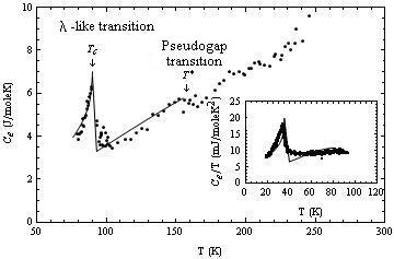
Figure 37: Temperature dependence of the specific heat of $HoBa_{2}Cu_{3}O_{7-\delta}$ measured near $T_{c}$ and above $T_{c}$ 238 . Solid line is the calculated curve for comparing with experimental points (black circles). According to Eq. (92), $C_{n}(T)$ is calculated by using the parameters $\varepsilon_{F}=0.12$ eV, $\varepsilon_{FI}=0.012$ eV, $f_{p}=f_{1}=0.3$, $f_{I}=f_{2}=0.7$, while superconducting contribution $C_{s}(T)$ to $C_{e}(T)$ is calculated by using the parameters $\rho_{B}=1.6\times 10^{19}\rm{cm^{-3}}$, $m_{B}=5m_{e}$, $\tilde{\mu}_{B}(T_{c})=1.6$ meV and $f_{s}=0.03$. The inset shows the calculated temperature dependence of $C_{e}(T)/T$ (solid line) compared with experimental $C_{e}(T)/T$ data for LSCO 33 (black circles). According to Eq. (92), $C_{n}(T)/T$ is calculated by using the parameters $\varepsilon_{F}=0.1$ eV $\varepsilon_{FI}=0.06$ eV, $f_{p}=f_{1}=0.4$, $f_{I}=f_{2}=0.6$, while $C_{s}(T)/T$ is calculated by using the parameters $\rho_{B}=1.4\times 10^{19}\rm{cm^{-3}}$, $m_{B}=5.4m_{e}$, $\tilde{\mu}_{B}(T_{c})=0.5$ meV and $f_{s}=0.012$.

We now examine more closely the temperature-dependent behavior of $C_{e}(T)$ in high-$T_{c}$ cuprates near $T_{c}$ and above $T_{c}$ by comparing the calculated results for $C_{e}(T)$ with experimental data. As $T$ approaches $T_{c}$ from below, the temperature dependences of $\tilde{\mu}_{B}$ and $\Delta_{B}$ are described by Eqs. (157) and (158). Essentially, the behavior of $C_{e}(T)$ at temperatures close to $T_{c}$ is determined by the following temperature derivaties of $\tilde{\mu}_{B}(T)$ and $\Delta_{B}(T)$ entering the second term of Eq. (VII.7): $\partial\tilde{\mu}_{B}(T)/\partial T=-a\tilde{\mu}_{B}(T_{c})(T_{c}-T)^{-0.5}/2\sqrt{T_{c}}$, $\partial\tilde{\mu}_{B}(T)^{2}/\partial T\simeq-a\tilde{\mu}_{B}(T_{c})^{2}(T_{c}-T)^{-0.5}/\sqrt{T_{c}}$ and $\partial\Delta^{2}_{B}(T)/\partial T=-2a\tilde{\mu}_{B}(T_{c})^{2}(T_{c}-T)^{-0.5}/\sqrt{T_{c}}$.

These temperature derivatives of $\tilde{\mu}_{B}$ and $\Delta_{B}$ in the expression for $C_{e}(T)$ give rise to a pronounced $\lambda$-like divergence at $T_{c}$, which is different from the BCS/BEC transition. By introducing the quantity of superfluid matter $\nu_{B}=N_{B}/N_{A}$ (where $N_{B}$ is the number of attracting bosonic Cooper pairs and $N_{A}$ is the Avogadro number, which is equal to the number of CuO₂ formula unit per unit molar volume) and the molar fraction of the superfluid bosonic carriers defined by $f_{s}=\nu_{B}/\nu$ (where $\nu=N/N_{A}$ is the amount of doped matter), we now write the molar specific heat of the superfluid Bose-liquid in high-$T_{c}$ cuprates as

$$C_{s}(T) = f_{s}\frac{C_{e}(T)}{\nu_{B}}=f_{s}\frac{D_{B}k_{B}N_{A}}{4\rho_{B}(k_{B}T)^{2}}\int^{\xi_{BA}}_{0}\sqrt{\varepsilon}\frac{d\varepsilon}{\sinh^{2}\frac{E_{B}(\varepsilon)}{k_{B}T}}\times$$

$$\times\left\{E^{2}_{B}(\varepsilon)+\frac{a\tilde{\mu}_{B}(T_{c})T}{2\sqrt{T_{c}}(T_{c}-T)^{0.5}}\left[\varepsilon-\tilde{\mu}_{B}(T_{c})\right]\right\}.$$

Here we have assumed that $\Omega/\nu_{B}=N_{B}v_{B}/\nu_{B}=v_{B}N_{A}$ and $v_{B}=1/\rho_{B}$. In doped cuprates the carriers are distributed between the polaronic band and the impurity band (with Fermi energy $\varepsilon_{FI}$) and the normal-state specific heat $C_{n}(T)$ above $T_{c}$ is calculated by considering three contributions from the excited components of Cooper pairs, the ideal Bose-gas of Cooper pairs and the unpaired carriers bound to impurities (see Eq. (92)). The total electronic specific heat $C_{e}(T)=C_{s}(T)+C_{n}(T)$ below $T_{c}$ is calculated and compared with the experimental data for $C_{e}(T)$ in cuprates (see Fig. 37). In so doing, the fraction $f_{p}$ of carriers residing in the polaronic band and the other fraction $f_{I}$ of carriers residing in the impurity band are taken into account in comparing the specific heat $C_{e}(T)$ with the experiment.

VIII.5 4. London Penetration Depth

In BCS-like pairing theories, the magnetic field penetration into the superconductor or the London penetration depth $\lambda_{L}(T)$ is determined within the two Fermi-liquid model. However, in bosonic superconductors the temperature dependence of the London penetration depth $\lambda_{L}(T)$ should be determined within the two Bose-liquid model 22 (in the case of 2D-holon superconductors this question was studied in Ref. 224 ) from the relation

$$\frac{\lambda_{L}(T)}{\lambda_{L}(0)}=\left[1-\frac{\rho_{n}(T)}{\rho_{B}}\right]^{-1/2},$$ (198)

where $\lambda_{L}(0)=(m_{B}c^{2}/4\pi\rho_{B}e^{*2})^{1/2}$, $c$ is the light velocity, $e^{*}=2e$ is the charge of Cooper pairs, $\rho_{B}=\rho_{s}+\rho_{n}$, $\rho_{s}$ and $\rho_{n}$ are the densities of the superfluid and normal parts of a Bose-liquid. The density of the normal part of a 3D Bose-liquid is determined from the expression 239

$$\rho_{n}=-\frac{1}{3m_{B}}\int\frac{dn_{B}}{dE_{B}}p^{2}\frac{4\pi p^{2}dp}{(2\pi\hbar)^{3}},$$ (199)

where $n_{B}=[\exp(E_{B}(k))/k_{B}T-1]^{-1}$, $p=\sqrt{2m_{B}\varepsilon}$. For the case $\gamma_{B}<\gamma^{*}_{B}$, the excitation spectrum of a 3D Bose-liquid becomes gapless below $T^{*}_{c}$. If $\gamma_{B}<<\gamma^{*}_{B}$, the excitation spectrum of such Bose-liquid will be phonon-like $E_{B}(\varepsilon)\simeq\sqrt{2\Delta_{B}\varepsilon}=v_{c}p$ at $T\leq T_{c}^{*}<T_{c}$. Then Eq. (199), after integration by parts, yields

$$\rho_{n}=\frac{2}{3\pi^{2}m_{B}\hbar^{3}v_{c}}\int^{\infty}_{0}\frac{p^{3}dp}{\exp[v_{c}p/k_{B}T]-1}=$$

$$=\frac{2(k_{B}T)^{4}}{3\pi^{2}m_{B}\hbar^{3}v^{5}_{c}}\Gamma(4)\zeta(4),$$ (200)

where $\Gamma(4)=3!$, $\zeta(4)=\pi^{4}/90$.

Substituting Eq. (VIII.5) into Eq. (198), we obtain

$$\frac{\lambda_{L}(T)}{\lambda_{L}(0)}=\Big{[}1-\Big{(}\frac{T}{T_{c}}\Big{)}^{4}\Big{]}^{-1/2}.$$ (201)

Equation (201) is in agreement with the well-known Gorter-Casimir law found earlier only empirically 30 , which is different from the exponential law predicted by BCS theory. At $\gamma_{B}<\gamma^{*}_{B}$, the expression (201) for $\lambda_{L}(T)/\lambda_{L}(0)$ holds at low temperatures ($T^{*}_{c}<<T_{c}$). While the $T$-dependence of $\lambda_{L}$ in 3D bosonic superconductors at $\Delta_{g}>k_{B}T$ can be approximately obtained after replacing $E_{B}(\varepsilon)$ by $\sqrt{\Delta^{2}_{g}+2\tilde{\mu}_{B}\varepsilon}\simeq\Delta_{g}+\tilde{\mu}_{B}\varepsilon/\Delta_{g}$ in Eq. (199) at small $\varepsilon$. In this case, evaluating the integral in Eq. (199) and using Eq. (198), we find

$$\frac{\lambda_{L}(T)}{\lambda_{L}(0)}=\Big{[}1-\left(\frac{\Delta_{g}(T)}{\tilde{\mu}_{B}(T)}\right)^{5/2}\left(\frac{T}{T_{c}}\right)^{3/2}\times$$

$$\times\exp\left(-\frac{\Delta_{g}(T)}{k_{B}T}\left(1-\frac{T}{T_{c}}\right)\right)\Big{]}^{-1/2}.$$ (202)

At $\gamma_{B}<\gamma^{*}_{B}$ and low temperatures the energy gap $\Delta_{g}$ in the excitation spectrum of a 2D Bose-liquid is vanishingly small. Therefore, $E_{B}(\varepsilon)$ may also be approximated by $E_{B}(\varepsilon)\approx\sqrt{2\tilde{\mu}_{B}\varepsilon}=v_{c}p$. Then the density of the normal part of a 2D Bose-liquid $\rho_{n}$ is defined as

$$\rho_{n}\simeq-\frac{1}{2m_{B}v_{c}}\int^{\infty}_{0}\frac{dn_{B}}{dp}p^{2}\frac{2\pi p}{(2\pi\hbar)^{2}}dp=$$

$$=-\frac{1}{4\pi m_{B}\hbar^{2}v_{c}}\left[n_{B}p^{3}\Big{|}^{\infty}_{0}-3\int^{\infty}_{0}n_{B}p^{2}dp\right]=$$

$$=\frac{3}{4\pi m_{B}\hbar^{2}v_{c}}\int^{\infty}_{0}\frac{p^{2}dp}{\exp[v_{c}p/k_{B}T]-1}=$$

$$=\frac{3(k_{B}T)^{3}}{4\pi m_{B}\hbar^{2}v_{c}^{4}}\Gamma(3)\zeta(3),$$ (203)

where $\Gamma(3)=2!$, $\zeta(3)=1.202$.

Substituting this expression into Eq. (198), we obtain

$$\frac{\lambda_{L}(T)}{\lambda_{L}(0)}=\left[1-\left(\frac{T}{T_{c}}\right)^{3}\right]^{-1/2}.$$ (204)

At $\Delta_{g}>>k_{B}T$, we can again assume that $E_{B}(\varepsilon)\simeq\sqrt{\Delta^{2}_{g}+2\tilde{\mu}_{B}\varepsilon}\simeq\Delta_{g}+\tilde{\mu}_{B}\varepsilon/\Delta_{g}$. For the case of 2D bosonic superconductors, we then obtain approximately the following law:

$$\frac{\lambda_{L}(T)}{\lambda_{L}(0)}=\Big{[}1-\left(\frac{\Delta_{g}(T)}{\tilde{\mu}_{B}(T)}\right)^{2}\left(\frac{T}{T_{c}}\right)\times$$

$$\times\exp\left(-\frac{\Delta_{g}(T)}{k_{B}T}\left(1-\frac{T}{T_{c}}\right)\right)\Big{]}^{-1/2},$$ (205)

which can be valid in some temperature range below $T_{c}$. The exact results for $\lambda_{L}(T)/\lambda_{L}(0)$ are obtained by numerical calculation of the integral in Eq. (199), which can be written as

$$\rho_{n}=\frac{\sqrt{2}m^{3/2}_{B}}{3\pi^{2}\hbar^{3}k_{B}T}\times$$

$$\times\int^{\xi_{BA}}_{0}\frac{\exp(\sqrt{(\varepsilon+\tilde{\mu}_{B})^{2}-\Delta^{2}_{B}}/k_{B}T)}{\Big{[}\exp(\sqrt{(\varepsilon+\tilde{\mu}_{B})^{2}-\Delta^{2}_{B}}/k_{B}T)-1\Big{]}^{2}}\varepsilon^{3/2}d\varepsilon.$$

We now turn to the experimental evidence for $\lambda_{L}(T)$ in high-$T_{c}$ cuprates. Experimental results on the London penetration depth in these high-$T_{c}$ materials 241 are in well agreement with Eq. (201) and at variance with exponential law predicted by the BCS theory. Further, the power law dependence $\lambda_{L}(T)\sim T^{2}$ is also observed in high-$T_{c}$ cuprates 240 . Such a behavior of $\lambda_{L}(T)$ also follows approximately from the relation (VIII.5). In addition, in some experiments 242 the power law dependence $\lambda_{L}(T)/\lambda_{L}(0)\sim(T/T)^{n}$ with $n=1.3-3.2$ were observed in accordance with the above theoretical predictions.

It is now interesting to compare the numerical results for $\lambda_{L}(T)/\lambda_{L}(0)$ and $(\lambda_{L}(0)/\lambda_{L}(T))^{2}$ obtained using Eqs. (VIII.5) and (198) with the experimental data in a wide temperature region which extends up to $T_{c}$. As can be seen in Fig. 38 and Fig. 39, the fits of Eqs. (VIII.5) and (198) to experimental data are quite good. Here we discuss the origins of the change in the slope of $\lambda_{L}(T)/\lambda_{L}(0)$ and $[\lambda_{L}(0)/\lambda_{L}(T)]^{2}$ observed near $T_{c}^{*}$ well below $T_{c}$ in two different films of YBCO 241 ; 243 and the other features, like oscillations at lower temperatures ($T<T_{c}^{*}$). According to the theory of Bose-liquid superconductivity, the change of the slope of $\lambda_{L}(T)$ in high-$T_{c}$ cuprates occurs at a crossover temperature $T^{*}_{c}$ which decreases with decreasing the thickness of the films of these materials. The changes of the slope of $\lambda_{L}(T)/\lambda_{L}(0)$ and $(\lambda_{L}(0)/\lambda_{L}(T))^{2}$ in thin films of YBCO were actually observed at $T^{*}_{c}\simeq 0.65T_{c}$ 241 and $T^{*}_{c}\simeq 0.55T_{c}$ 243 , respectively. In particular, a first-order phase transition from $A$-like superconducting phase (pair condensate state of Cooper pairs) to $B$-like superconducting phase (single particle condensate state of Cooper pairs) occurs in the bulk of a YBCO film at $T_{c}^{*}\simeq 0.55T_{c}$, while such a phase transition occurs on 2D surfaces at $T=T_{c}^{*}=0$. It follows that crossover temperature $T_{c}^{*}$ near surfaces of a YBCO film decreases rapidly, thus indicating that surfaces actually tend to stabilize the remnant $A$-like superconducting phase below the bulk crossover temperature $T_{c}^{*}\simeq 0.55T_{c}$. Because the crossover from 3D to 2D superconductivity regime near surfaces would progressively shift $T_{c}^{*}$ towards low-temperature region. Measurements of the London penetration depth $\lambda_{L}$ on the YBCO film 243 seem to indicate the coexistence of competing two Bose condensates (i.e. the dominant single-particle condensate coexists with the persisting pair condensate) of bosonic Cooper pairs below $T_{c}^{*}\sim 0.55T_{c}$ due to surface effects. Apparently, the competitions between coexisting single particle and pair condensate states of such composite bosons near surfaces can give rise to additional multiple features, like oscillations in experimental measurements of $[\lambda_{L}(0)/\lambda_{L}(T)]^{2}$, at $T<T_{c}^{*}\sim 0.55T_{c}$ 243 .

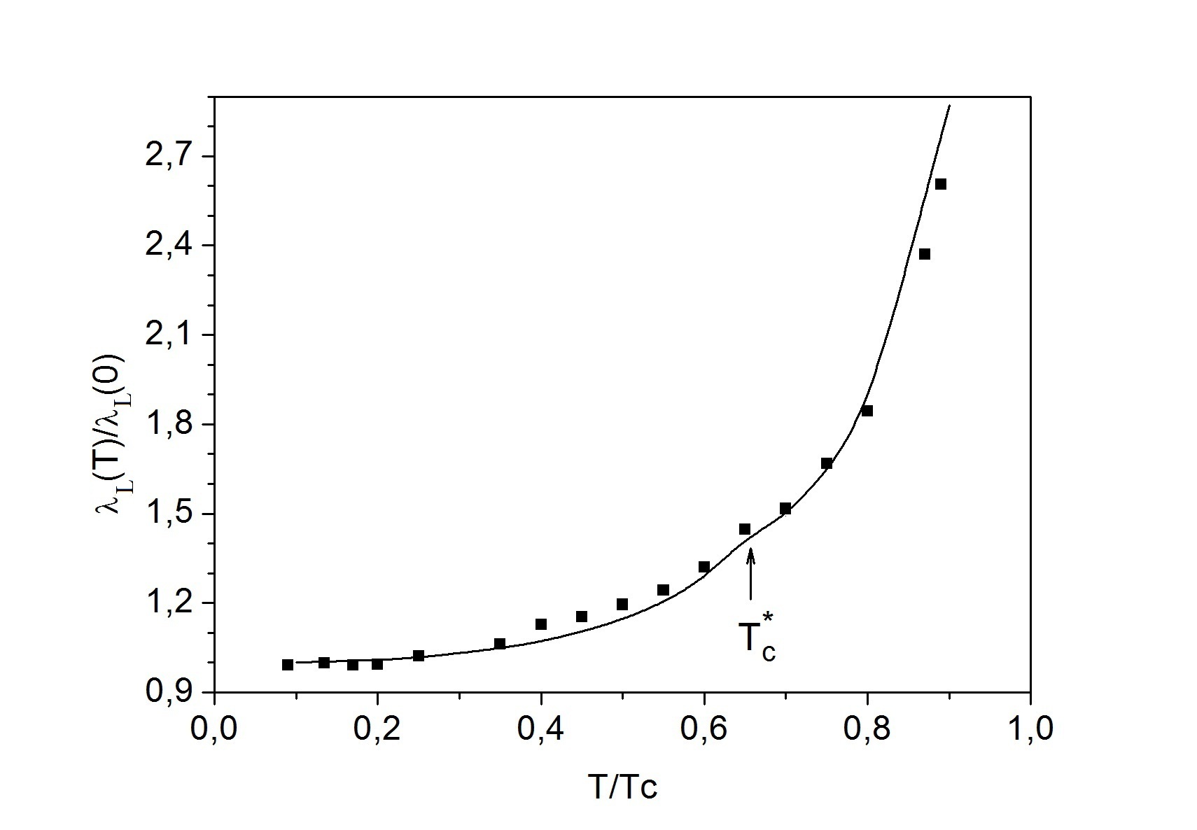
Figure 38: Temperature dependence of $\lambda_{L}(T)/\lambda_{L}(0)$ (solid line) is calculated by using Eqs. (VIII.5) and (198) with the fitting parameters $\rho_{B}\simeq 1.14\times 10^{19}\rm{cm^{-3}}$, $m_{B}=4.9m_{e}$, $\xi_{BA}=0.07$ eV and compared with experimental data ($\blacksquare$) for thin film of YBCO 241 . $T^{*}_{c}$ marks the first-order phase transition temperature at which the energy gap $\Delta_{g}$ vanishes in the excitation spectrum of 3D Bose-liquid of Cooper pairs.

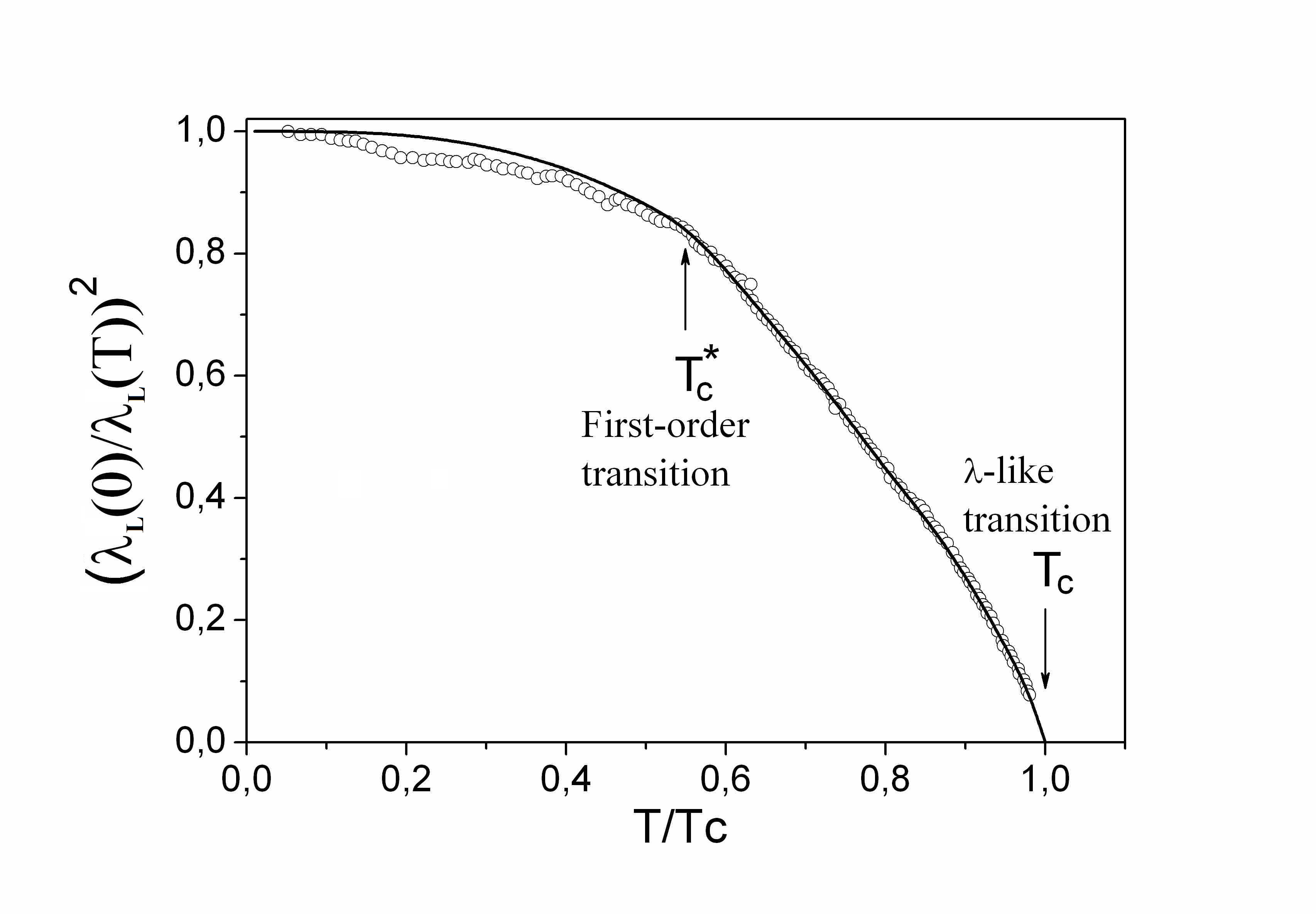
Figure 39: Temperature dependence of $(\lambda_{L}(0)/\lambda_{L}(T))^{2}$ (solid line) is calculated by using Eqs. (VIII.5) and (198) with the fitting parameters $\rho_{B}\simeq 1.29\times 10^{19}\rm{cm^{-3}}$, $m_{B}=5m_{e}$, $\xi_{BA}=0.08$ eV and compared with experimental data ($\circ$) for YBCO film 243

In the absence of a satisfactory microscopic theory of unconventional superconductivity in high-$T_{c}$ cuprates, Orbach-Werbig et al. 243 have started to compare their own key experimental results for the London penetration depth with the BCS-like (two-gap) theories. However, the explanation of the low- and high-temperature behaviors of $[\lambda_{L}(0)/\lambda_{L}(T)]^{2}$ in terms of two different (large and small) BCS-like gaps seems to be inadequate, and a phase transition, which is responsible for the change in the slope of $[\lambda_{L}(0)/\lambda_{L}(T)]^{2}$ observed at $T\sim 0.55T_{c}$ in YBCO 243 had remained unidentified. While the above theory of Bose-liquid superconductivity explains naturally the important experimental results of Ref. 243 . As a matter of fact, the first-order phase transition in a YBCO film occurs near $T_{c}^{*}\sim 0.55T_{c}$ (Fig. 39) and is accompanied by the change in the slope of $[\lambda_{L}(0)/\lambda_{L}(T)]^{2}$.

VIII.6 5. Critical current and superfluid density

We now discuss the main critical parameters in high-$T_{c}$ cuprate superconductors and show that the kink-like feature of the bosonic superconducting order parameter $\Delta_{SC}(T)=\Delta_{B}(T)$ is responsible for the kink-like behavior of the critical current $J_{c}(T)$ destroying superconductivity in these materials. The critical current density in bosonic superconductors is given by

$$J_{c}(T)=2e\rho_{s}(T)v_{c}(T),$$ (207)

where $\rho_{s}(T)=\rho_{B}-\rho_{n}$ is the superfluid density, $\rho_{n}$ is the density of the normal part of a 3D Bose-liquid determined from Eq. (VIII.5), $v_{c}(T)=\sqrt{[\tilde{\mu}_{B}(T)+\Delta_{g}(T)]/m_{B}}$ is the critical velocity of superfluid carriers (bosonic Cooper pairs).

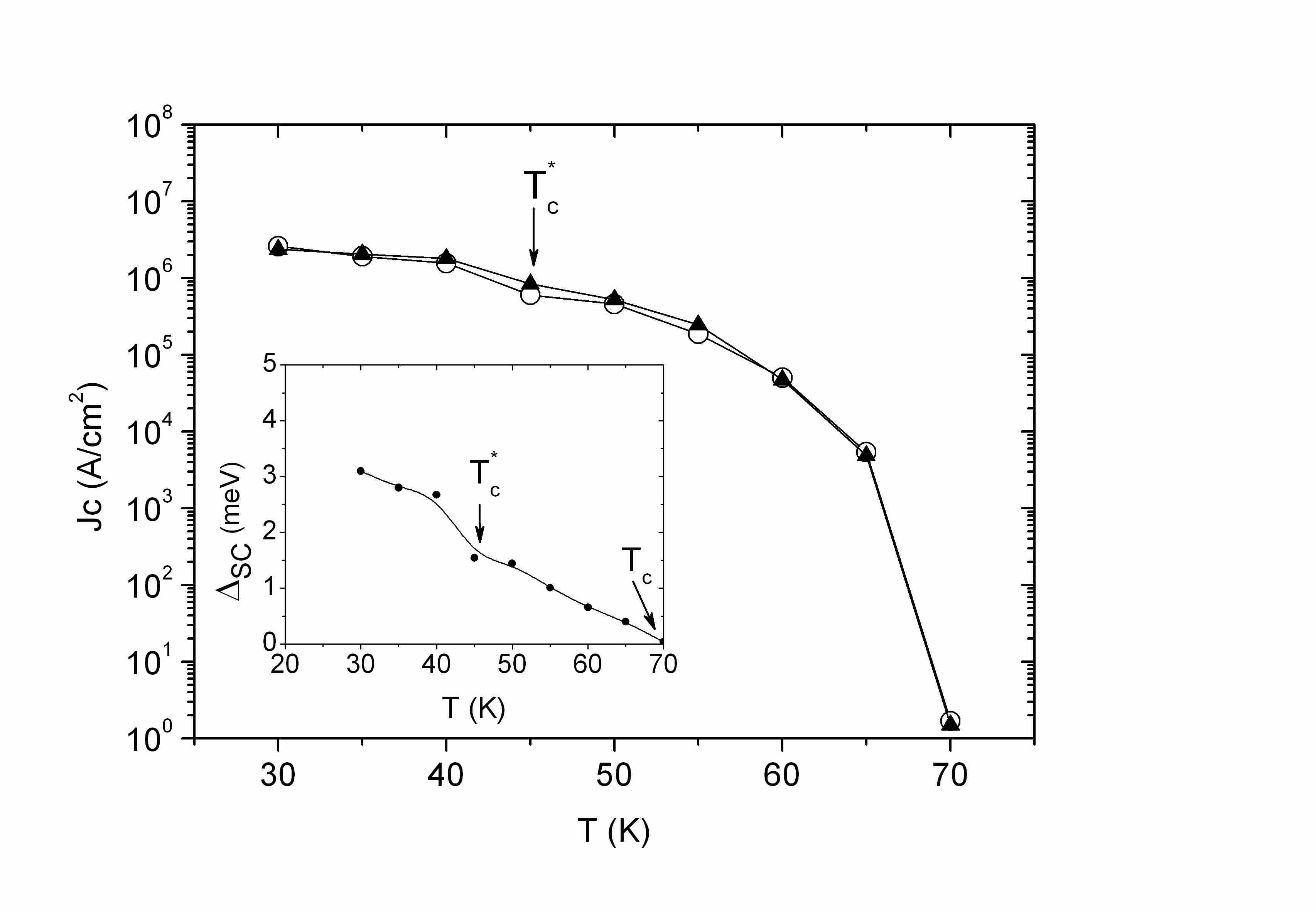
Figure 40: Temperature dependence of the critical current density $J_{c}$ measured in YBCO film and fitted by using Eq. (207). The solid line is the best fit of Eq. (207) ($\blacktriangle$) to the experimental data ($\circ$) for YBCO film 244 using the parameters $\rho_{B}\simeq 0.8\times 10^{19}\rm{cm^{-3}}$, $m_{B}=4.6m_{e}$, and $\xi_{BA}=0.08$ eV. The inset shows the kink-like behavior of $\Delta_{SC}(T)$ near the characteristic temperature $T^{*}_{c}$.

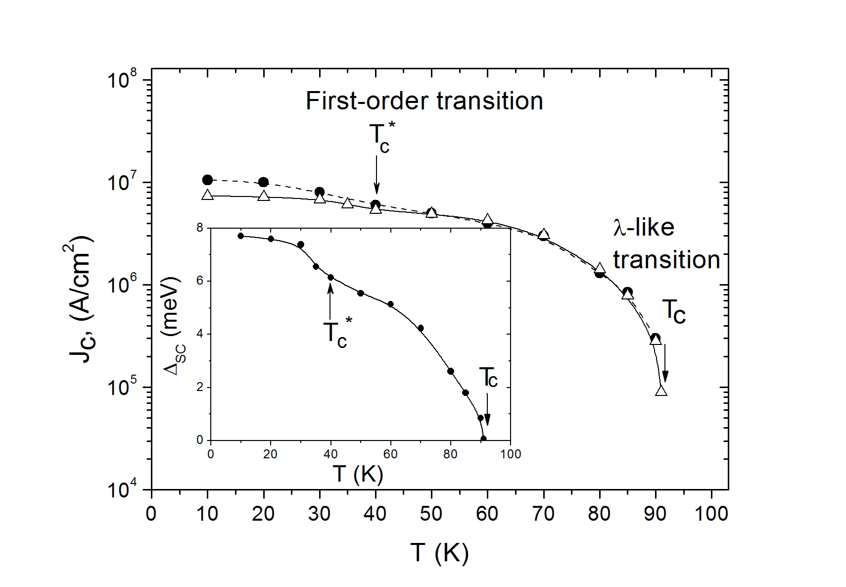
Figure 41: Temperature dependence of $J_{c}$ measured in YBCO film ($\bullet$). The solid line is the best fit of Eq. (207) ($\triangle$) to the experimental data ($\bullet$) for YBCO film 245 using the parameters $\rho_{B}\simeq 1.41\times 10^{19}\rm{cm^{-3}}$, $m_{B}=5.0m_{e}$ and $\xi_{BA}=0.08$ eV. The inset shows the kink-like behavior of $\Delta_{SC}(T)$ near $T^{*}_{c}$.

The superfluid density $\rho_{s}$ and the critical velocity $v_{c}$ of bosonic Cooper pairs in unconventional superconductors (which are bosonic superconductors), should be determined accoding to the above microscopic theory of superfluid Bose-liquid and not accoding to the theory of superfluid Fermi-liquid (as it accepted in BCS-like pairing theory). Our calculated results for $J_{c}(T)$ are compared with the experimental results obtained for two different YBCO films 244 ; 245 . As may be seen in Figs. 40 and 41, the temperature dependences of our calculated $J_{c}(T)$ for these high-$T_{c}$ cuprates are in good agreement with the experimental data 244 ; 245 (see Figs. 40 and 41). Most importantly, as $T$ approaches the characteristic temperature $T^{*}_{c}$ from above, the unusual temperature dependences (upward trends) of $J_{c}(T)$ in two different YBCO films were observed near $T^{*}_{c}\simeq 0.45T_{c}$ 244 and $T^{*}_{c}\simeq 0.40T_{c}$ 245 . Such kink-like behaviors of $J_{c}(T)$ in two different YBCO films shown in Figs. 40 and 41 are associated with the sharp increase of $\Delta_{B}(T)$ at the vanishing of the gap $\Delta_{g}$ in $E_{B}(k)$ near $T_{c}^{*}$ leading to the jump-like increasing of the superfluid density $\rho_{s}(T)$ and the critical velocity $v_{c}(T)$ of superfluid carriers.

VIII.7 6. Lower and upper critical magnetic fields

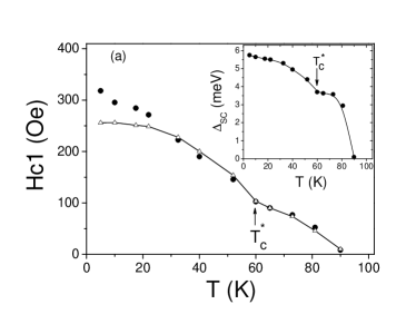
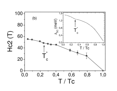
Figure 42: Temperature dependences of the critical magnetic fields $H_{c1}(T)$ and $H_{c2}(T)$ measured in superconducting cuprates. (a) Solid line is the fit of equation (208) ($\triangle$) to the experimental data ($\bullet$) for $H_{c1}(T)$ in YBCO 246 using the fitting parameters $\rho_{B}\simeq 1.7\times 10^{19}\rm{cm^{-3}}$, $m^{*}_{B}=4.4m_{e}$, $R_{w}=0.02cm$ and $\xi_{BA}=0.07$ eV. (b) Solid line is the fit of equation (210) ($\circ$) to the experimental data ($\blacksquare$) for $H_{c2}(T)$ in Bi-2201 249 using the fitting parameters $\rho_{B}\simeq 0.106\times 10^{19}\rm{cm^{-3}}$, $m^{*}_{B}=5.2m_{e}$, $R_{w}=0.5\times 10^{-3}cm$ and $\xi_{BA}=0.075$ eV. Insets show the kink-like behaviors of $\Delta_{SC}(T)$ near $T^{*}_{c}$.

The other distinctive superconducting properties of high-$T_{c}$ cuprates not encountered before in conventional superconductors are the unusual temperature dependences of their lower and upper critical magnetic fields. We show that the kink-like features of $\Delta_{SC}(T)$ and $J_{c}(T)$ strongly influence the temperature dependences of the critical magnetic fields near $T^{*}_{c}$, as observed in high-$T_{c}$ cuprates 246 ; 247 ; 248 ; 249 .

The lower critical magnetic field $H_{c1}$ is determined from the relation

$$H_{c1}(T)=\frac{\ln\chi(T)}{\sqrt{2}\chi(T)}H_{c}(T),$$ (208)

where $\chi(T)=\lambda_{L}(T)/\xi_{c}(T)$ is the Ginzburg-Landau parameter, $\xi_{c}(T)=\hbar/\sqrt{2m_{B}\Delta_{B}(T)}$ is the coherence length in bosonic superconductors, $H_{c}(T)$ is the thermodynamic critical magnetic field, which can be defined as 2

$$H_{c}(T)=4\pi R_{w}J_{c}(T)/c,$$ (209)

$R_{w}$ is the radius of a superconducting wire.

The upper critical magnetic field is given by

$$H_{c2}(T)=\sqrt{2}\chi(T)H_{c}(T).$$ (210)

From Eqs. (208), (209) and (210), it follows that the kink-like temperature dependences of $\Delta_{SC}(T)$ and $J_{c}(T)$ give rise to a kink in the temperature dependence of both $H_{c1}$ and $H_{c2}$ near the first-order phase transition temperature $T^{*}_{c}$. Since the critical magnetic fields $H_{c1}(T)$ and $H_{c2}(T)$, just like $\Delta_{B}(T)$ or $J_{c}(T)$, increase abruptly near $T_{c}^{*}$ (where the first-order transition from A-like superconducting phase to B-like superconducting phase occurs) with decreasing $T$ and they manifest positive (or upward) curvature in the vicinity of $T_{c}^{*}$. Actually, such distinctive temperature dependences of $H_{c1}$ and $H_{c2}$ were observed in high-$T_{c}$ cuprates 246 ; 247 ; 248 ; 249 in accordance with the above predictions of the microscopic theory of superfluid Bose-liquid. Our calculated results for $H_{c1}(T)$ and $H_{c2}(T)$ are compared with the experimental results obtained for YBCO 246 and $\rm{Bi_{2+\emph{x}}Sr_{2-\emph{x}}CuO_{6}}$ (Bi-2201) 249 . The kink-like behaviors of $H_{c1}(T)$ (in YBCO) and $H_{c2}(T)$ (in Bi-2201 with $T_{c}\lesssim 15$ K) near $T_{c}^{*}$ are shown in Fig. 42. Our numerical results for $H_{c1}(T)$ and $H_{c2}(T)$ show reasonable agreement with the experimental data for YBCO (Fig. 42a) and for Bi-2201 (Fig. 42b). Thus, the validity of the microscopic theory of novel Bose-liquid superconductivity in high-$T_{c}$ cuprates are also confirmed in experiments on measuring critical magnetic fields $H_{c1}(T)$ and $H_{c2}(T)$.

VIII.8 7. Critical superconducting transition temperatures in 3D and 2D high-$T_{c}$ cuprates

Another most important and distinctive critical parameter in high-$T_{c}$ cuprates is the $\lambda$-like superconducting transition temperature $T_{c}$. According to the experimental observations 33 ; 59 ; 60 ; 250 , the superconducting transition in these systems is more $\lambda$-like than the usual BEC transition and is fundamentally different from the step-like BCS transition. On the basis of the analysis presented in Sec.VII, we can determine the critical temperature $T_{c}$ of the $\lambda$-like superconducting transition in 3D systems. Actually, polaronic Cooper pairs in these materials are pre-existing composite bosons and such Cooper pairs condense into a Bose superfluid at a $\lambda$-like transition temperature. Given the above (subsection A), we can assume that $\xi_{BA}=\hbar\omega_{0}$. In the intermediate coupling regime ($0.3<\gamma_{B}<1$), the superconducting transition temperature in a 3D Bose-liquid of Cooper pairs can be roughly defined as

$$T_{c}=T^{3D}_{c}\simeq T^{*}_{BEC}\left[1+c_{0}\gamma_{B}\sqrt{\sqrt{2}k_{B}T^{*}_{BEC}/\hbar\omega_{0}}\right],$$

where $T^{*}_{BEC}=3.31\hbar^{2}\rho^{2/3}_{B}/k_{B}m^{*}_{B}$ and $m^{*}_{B}$ is determined from Eq. (181)

Further, the superconducting transition temperature in the weak coupling regime ($\gamma_{B}<0.3$) is given by

$$T^{3D}_{c}\simeq T^{*}_{BEC}\left[1+c_{0}\gamma_{B}\sqrt{k_{B}T^{*}_{BEC}/\hbar\omega_{0}}\right].$$ (212)

Unlike the case of 3D systems, the critical temperature of the superconducting transition in 2D systems for arbitrary $\gamma_{B}$ is determined according to the formula

$$T^{2D}_{c}=-\frac{T^{*}_{0}}{ln[1-\exp(-2\gamma_{B}/(2+\gamma_{B}))]},$$ (213)

where $T^{*}_{0}=2\pi\hbar^{2}\rho_{B}/k_{B}m^{*}_{B}$,

Thus, both $T_{c}$ and $T^{2D}_{c}$ in high-$T_{c}$ cuprates are mainly controlled by $\rho_{B}$ and $\gamma_{B}$.

VIII.9 8. Unusual isotope effects on $T_{c}$

We argue that the polaronic effects gives rise to the unexpected (i.e. unusual) isotope effects on $T_{c}$ in high-$T_{c}$ cuprates, since the mass of large polarons $m_{p}(>m_{e})$ and the optical phonon energy $\hbar\omega_{0}$ entering into the expression for $T_{c}$ could be the origin of such isotope effects on $T_{c}$. In order to study the polaronic isotope effect on $T_{c}$, the mass of polarons is determined from Eq. (97) and the expression for $T^{*}_{BEC}$ should be written as

$$T^{*}_{BEC}=\frac{3.31\hbar^{2}\rho^{2/3}_{B}(1-\rho_{B}\tilde{V}_{B}/\xi_{BR})}{2k_{B}m_{e}(1+\alpha_{F}/6)},$$ (214)

where $\alpha_{F}=(e^{2}/\hbar\tilde{\varepsilon})\sqrt{m_{e}/2\hbar\omega_{0}}$, $\hbar\omega_{0}=\hbar(2\kappa(\frac{1}{M}+\frac{1}{M^{\prime}}))^{1/2}$, $M(=M_{O}$ or $M_{Cu})$ and $M^{\prime}(=M_{Cu}$ or $M_{O})$ are the masses of the oxygen $O$ and copper atoms in the cuprates.

For $Y$- and Bi-based cuprates, we use Eq. (VIII.8) for studying the isotope effects on $T_{c}$. This equation can now be written as

$$T_{c}=\frac{a_{2}[1+c_{1}a^{1/2}_{2}\mu^{1/4}(1+a_{1}\mu^{1/4})^{-1/2}]}{1+a_{1}\mu^{1/4}},$$ (215)

where $a_{1}=(e^{2}\sqrt{m_{e}}/6\sqrt{2}\hbar^{3/2}\tilde{\varepsilon}(2\kappa))^{1/4}$, $c_{1}=c_{0}\gamma_{B}\kappa^{-1/4}\sqrt{k_{B}/\hbar}$, $a_{2}=3.31\hbar^{2}\rho^{2/3}_{B}[1-\rho_{B}\tilde{V}_{B}/\xi_{BR}]/2k_{B}m_{e}$, $\mu=M_{O}M_{Cu}/(M_{O}+M_{Cu})$.

Next the exponent of the isotope effect on $T_{c}$ is defined as

$$\alpha_{T_{c}}=-\frac{d\ln T_{c}}{d\ln M}.$$ (216)

Using Eqs. (215) and (216), we then obtain

$$\alpha_{T_{c}}=\frac{\mu^{1/4}A_{c}(\mu)}{4(1+M/M^{\prime})a_{2}B_{c}(\mu)},$$ (217)

where $A_{c}(\mu)=a_{1}a_{2}(1+a_{1}\mu^{1/4})^{-1}-c_{1}a^{3/2}_{2}(1+a_{1}\mu^{1/4})^{-1/2}+\frac{3}{2}c_{1}a_{1}a^{3/2}_{2}\mu^{1/4}(1+a_{1}\mu^{1/4})^{-3/2}$, $B_{c}({\mu})=1+c_{1}a^{1/2}_{2}\mu^{1/4}(1+a_{1}\mu^{1/4})^{-1/2}$.

As seen from Eqs. (215) and (217), the superconducting transition temperature $T_{c}$, the isotope shifts $\Delta T_{c}$ and the exponents $\alpha^{O}_{T_{c}}$ and $\alpha^{Cu}_{T_{c}}$ of the oxygen and copper isotope effects on $T_{c}$ basically depend on the parameters $\rho_{B}$, $\gamma_{B}$, $\omega_{0}$, $\tilde{\varepsilon}$ and $\mu$. The parameter $\kappa$ is fixed at the value estimated for the oxygen and copper unsubstituted compound using the relation $\kappa=\mu\omega^{2}_{0}/2$. Further, two of the above parameters ($\omega_{0}$ and $\tilde{\varepsilon}$) have been already determined experimentally and are not entirely free (fitting) parameters for the high-$T_{c}$ cuprates. Equations (215) and (217) allow us to determine $T_{c}$, oxygen isotope shift $\Delta T_{c}^{O}=T_{c}(^{18}O)-T_{c}(^{16}O)$, copper isotope shift $\Delta T_{c}^{Cu}=T_{c}(^{65}Cu)-T_{c}(^{63}Cu)$, $\alpha^{O}_{T_{c}}$ and $\alpha^{Cu}_{T_{c}}$ in various high-$T_{c}$ cuprates. Since the vibrations of the lightest ion (i.e. oxygen ion) is expected to make the largest contribution to the isotope shift of $T_{c}$ in high-$T_{c}$ cuprates, the isotope-effect studies concentrated on measuring the oxygen isotope-effect on $T_{c}$. There are much experimental evidences for the unusual isotope effects on $T_{c}$ in high-$T_{c}$ cuprates 46 ; 175 ; 176 . Most of the experiments showed that the oxygen isotope effect on $T_{c}$ in $\rm{Y}$- and $\rm{La}$- based cuprates is absent or becomes small positive 178 ; 181 ; 251 and even negative 252 , compared to the BCS prediction, $T_{c}\sim M^{-\alpha}$ with $\alpha=+0.5$. Below, we will show that Eqs. (215) and (217) predict the existence of the novel oxygen isotope effect on $T_{c}$ observed in various high-$T_{c}$ cuprates.

For the given ionic masses $M$ and $M^{\prime}$, Eqs. (215) and (217) have to be solved simultaneously and self-consistently to determine $T_{c}$ and the isotope effect on $T_{c}$. Then, replacing in these equations the oxygen ion mass ${}^{16}\rm{O}$ by its isotope ${}^{18}\rm{O}$ mass and keeping all other parameters identical to the case ${}^{16}\rm{O}$, $T_{c}$ is calculated again and the isotope shift $\Delta T_{c}^{O}=T_{c}(^{18}O)-T_{c}(^{16}O)$ is calculated for ${}^{16}\rm{O}\longrightarrow^{18}\rm{O}$ substitution. The isotope shift $\Delta T_{c}^{Cu}=T_{c}(^{65}Cu)-T_{c}(^{63}Cu)$ is calculated in the same manner for ${}^{63}\rm{Cu}\longrightarrow^{65}\rm{Cu}$ substitution. We will now present our theoretical results, which are compared with the existing experimental data. In particular, with fitting parameters $\rho_{B}=2.5\cdot 10^{19}\rm{cm^{-3}}$, $\hbar\omega_{0}=0.022$ eV, $\tilde{\varepsilon}=4$ and $\rho_{B}\tilde{V}_{B}/\xi_{BR}=0.1$, one can explain the oxygen isotope effect on $T_{c}$ observed in $\rm{YBa_{2}Cu_{4}O_{8}}$ 181 . In this case, we obtain $T_{c}\simeq 81.23K$, $\Delta T_{c}^{O}\simeq-0.51K$ and $\alpha_{T_{c}}^{O}\simeq 0.054$, which are in good agreement with the experimental results $T_{c}=81K$, $\Delta T_{c}^{O}=-0.47K$ and $\alpha_{T_{c}}^{O}=0.056$ reported in Ref. 181 for $\rm{YBa_{2}Cu_{4}O_{8}}$.

In order to explain the other experiments on oxygen isotope effect on $T_{c}$ in various high-$T_{c}$ cuprates, we took $\rho_{B}=1.76\cdot 10^{19}\rm{cm^{-3}}$, $\hbar\omega_{0}=0.02$ eV, $\tilde{\varepsilon}=2.1$, $\rho_{B}\tilde{V}_{B}/\xi_{BR}=0.05$ for LSCO; $\rho_{B}=2.5\cdot 10^{19}\rm{cm^{-3}}$, $\hbar\omega_{0}=0.023$ eV, $\tilde{\varepsilon}=4.6$, $\rho_{B}\tilde{V}_{B}/\xi_{BR}=0.1$ for YBCO; $\rho_{B}=2.4\cdot 10^{19}\rm{cm^{-3}}$, $\hbar\omega_{0}=0.038$ eV, $\tilde{\varepsilon}=5.7$, $\rho_{B}\tilde{V}_{B}/\xi_{BR}=0.25$ for $\rm{Bi_{2}Sr_{2}CaCu_{2}O_{8}}$ (Bi-2212); $\rho_{B}=2.8\cdot 10^{19}\rm{cm^{-3}}$, $\hbar\omega_{0}=0.042$ eV, $\tilde{\varepsilon}=5$, $\rho_{B}\tilde{V}_{B}/\xi_{BR}=0.11$ for $\rm{Bi_{2}Sr_{2}Ca_{2}Cu_{3}O_{10}}$ (Bi-2223); $\rho_{B}=3.2\cdot 10^{19}\rm{cm^{-3}}$, $\hbar\omega_{0}=0.075$ eV, $\tilde{\varepsilon}=8$, $\rho_{B}\tilde{V}_{B}/\xi_{BR}=0.36$ for $\rm{Bi_{1.6}Pb_{0.4}Sr_{2}Ca_{2}Cu_{3}O_{10}}$ (Bi-2223 (Pb)). The calculated results for $T_{c}$ and $\alpha_{T}^{O}$ are also in reasonable quantitative agreement with the experimental values of $T_{c}$ and $\alpha_{T_{c}}^{O}$ in these high-$T_{c}$ cuprates (see Table VI).

Table 6: Experimental and theoretical values of the superconducting transition temperature $T_{c}$ and oxygen isotope shift exponent $\alpha_{T_{c}}^{O}$ in various high-$T_{c}$ cuprates.

		Experiment		Theory
Cuprate	$T_{c}$,	$\alpha^{O}_{T_{c}}$	Refs.	$\gamma_{B}$	$T_{c}$,	$\alpha^{O}_{T_{c}}$
compounds	K				K
LSCO	38	0.13	[251]	0.35	38	0.11
YBCO	91	0.040	[251]	0.55	91	0.041
YBa2Cu4O8	81	0.056	[181]	0.50	81	0.054
Bi-2212	75	0.034	[251]	0.38	75	0.035
Bi-2223	110	0.023	[251]	0.59	110	0.023
Bi-2223 (Pb)	108	-0.013	[252]	0.80	108	-0.013

VIII.10 9. Gapless bosonic excitations below $T_{c}$ and vortex-like excitations and diamagnetism above $T_{c}$

The origins of the gapless superconductivity and gapless excitations in unconventional superconductors are often misinterpreted in terms of the BCS-like $p$- or $d$-wave pairing scenarios and are still invariably attributed to the nodes of $p$- or $d$-wave BCS-like gap without clarifying the fermionic or bosonic nature of Cooper pairs and the relevant mechanisms of superconductivity. According to the above theory of a 3D superfluid Bose-liquid, the gapless excitations in high-$T_{c}$ cuprates are explained naturally by the absence of the energy gap $\Delta_{g}$ in the excitation spectrum $E_{B}(k)$ of such a Bose-liquid. Here the key discovery is that the novel gapless superconductivity is associated with the gapless excitation spectrum of a 3D superfluid Bose condensate of Cooper pairs below $T^{*}_{c}$. We argue that the gapless excitations observed in unconventional cuprate superconductors are intimately related to the vanishing of the bosonic excitation gap $\Delta_{g}$ at $T\leqslant T^{*}_{c}$ (where $T^{*}_{c}<T_{c}$ for $\gamma_{B}<<1$ and $T^{*}_{c}<<T_{c}$ for $\gamma_{B}\sim 1$) and not to vanishing of the BCS-like fermionic excitation gap $\Delta_{F}$ discussed in some $p$- and $d$-wave pairing models. Actually, in 3D Bose systems the transition from pair condensation regime to single particle condensation regime at the vanishing of the gap $\Delta_{g}$ explains the experimental observation of the existence of gapless excitations below some characteristic temperature $T_{c}^{*}<<T_{c}$ 253 as well as their nonexistence above $T_{c}^{*}$ up to $T_{c}$ in high-$T_{c}$ cuprates.

We now discuss the origins of the vortex-like excitations and diamagnetism above $T_{c}$. Equations (VIII.8) and (213) allow us to determine the critical superconducting transition temperatures in the bulk and at the quasi-2D grain boundaries in high-$T_{c}$ cuprates. Using the parameters $m_{p}\simeq 2.0m_{e}$, $m_{B}=2m_{p}$, $m^{*}_{B}\simeq 1.1m_{B}$ and $\rho_{B}\simeq 3\times 10^{19}\rm{cm^{-3}}$ for 3D high-$T_{c}$ cuprates, we find $T^{*}_{BEC}\simeq 64.3$ K. We then estimate $T_{c}$ by assuming that $\hbar\omega_{0}=0.03$ eV and $\gamma_{B}=0.7$. In this case, Eq. (VIII.8) predicts $T_{c}\simeq 1.508T^{*}_{BEC}\simeq 97K$. We can use the parameters $m_{p}\simeq 3m_{e}$, $m_{B}=2m_{p}$, $m^{*}_{B}\simeq 1.1m_{B}$ and $\rho_{B}\simeq 1.7\times 10^{13}\rm{cm^{-3}}$ for quasi-2D grain boundaries in high-$T_{c}$ cuprates to estimate the values of $T_{0}^{*}$ and $T_{c}^{2D}$ using Eq. (213). By taking $\gamma_{B}=0.7$ for quasi-2D grain boundaries, we then obtain $T^{*}_{0}\simeq 143$ K and $T^{2D}_{c}\simeq 1.105T_{0}^{*}\simeq 158$ K. We see that the highest $T_{c}$ is expected in quasi-2D Bose systems.

From the above considerations, it follows that the superconducting transition temperature in the cuprates is higher at quasi-2D grain boundaries than in the bulk and the residual 2D Bose-liquid superconductivity persists at quasi-2D grain boundaries in the temperature range $T_{c}<T<T_{v}(=T^{2D}_{c})$, i.e., the stability of high-$T_{c}$ superconductivity in cuprates is greater in quasi-2D than in 3D systems. Therefore, the vortex-like Nernst signals observed in high-$T_{c}$ cuprates from the underdoped to overdoped regime 35 ; 254 ; 255 are caused by the destruction of the bulk Bose-liquid superconductivity in the 3D-to-2D crossover region and are associated with the existence of the residual Bose-liquid superconductivity at quasi-2D grain boundaries rather than with other effects (e.g., pseudogap and superconducting fluctuation effects). More importantly, the experimental results presented in Ref. 256 agree with these predictions. Other experimental results also indicate 257 that the residual superconductivity in high-$T_{c}$ cuprates above $T_{c}$ cannot be attributed to the superconducting fluctuation. These results prohibit from using the BCS-like theory (i.e. superfluid Fermi-liquid picture) to understand the superconducting transitions in high-$T_{c}$ cuprates.

There are also some confusions in the literature about the origins of vortex-like and diamagnetic states, which have been found in unconventional cuprate superconductors above $T_{c}$ 254 ; 255 ; 258 ; 259 . We argue that the vortex-like Nernst signals are not associated with the diamagnetic signal persisting above $T_{c}$, since the vortex-like state should persist up to superconducting transition temperature $T^{2D}_{c}=T_{v}$ at quasi-2D grain boundaries. While the diamagnetism above $T_{c}$ is associated with the formation of bosonic Cooper pairs (with zero spin) and would persist in underdoped and optimally doped cuprates up to pseudogap temperatures $T^{*}>>T_{c}$ and $T^{*}\gtrsim T_{c}$, respectively.

Finally, it is interesting to predict that the superconducting transition temperature can reach up to the room temperature in some unconventional quasi-2D cuprate materials with increasing $\gamma_{B}$ and $\rho_{B}$ (the density of the attractive part of bosonic Cooper pairs). If we assume $\rho_{B}=3\cdot 10^{13}cm^{-2}$ and $\gamma_{B}=0.76$ for such systems, we find $T^{*}_{0}\simeq 253K$ and $T^{2D}_{c}\simeq 1.164T^{*}_{0}\simeq 294$ K. It follows that the room temperature superconductivity can be realized in ultra-thin 2D films or on the surfaces (e.g. grain boundaries and interfaces) of cuprate superconductors and other related materials.

VIII.11 10. The full and relevant phase diagram of high-$T_{c}$ cuprates

The above presented microscopic theory of pseudogap phenomena and unconventional Bose-liquid superconductivity in high-$T_{c}$ cuprates allows us to construct a full and relevant phase diagram of these doped CT-type Mott insulators. The richness of the electronic properties of cuprate materials from lightly doped to overdoped region seems to be inevitably related to the complexity of their phase diagram and, the key probably lies in this complexity. In the lightly doped cuprates, the strong and unconventional electron-phonon interactions are responsible for the existence of localized carriers and (bi)polaronic insulating state. Specifically, a small level of doping (e.g., $x\simeq 0.02-0.03$ 89 ; 249 ) results in the disappearance of AF order, the system undergoes a transition from the AF insulator to the (bi)polaronic insulator. Upon further doping, the cuprate compounds are converted into a pseudogap metal (above $T_{c}$) or a non-BCS (bosonic) high-$T_{c}$ superconductor (below $T_{c}$) 260 . We now identify the genuine phase diagram of high-$T_{c}$ cuprate superconductors starting from the unusual Fermi- liquid state and the superfluid Bose-liquid state. Our results indicate (see Sec. III) that the normal state of underdoped to overdoped cuprates cannot be regarded as a conventional Fermi liquid phase. Since the normal state of high-$T_{c}$ cuprates exhibits a pseudogap behavior below the upper characteristic temperature $T_{p}$ and the curve $T_{p}$ above $T_{c}$ separates the pseudogap and normal metal phases. The upper $T_{p}$ curve crosses the dome-shaped $T_{c}$ curve at around the optimal doping level (in YBCO) or overdoping level (in LSCO and Bi-2212), and fall down to $T=0$ at the QCP inside the superconducting phase. Below $T_{c}$ the curve $T_{p}$ separates the phase diagram of high-$T_{c}$ cuprates into two fundamentally different superconducting states. Such a pseudogap phase boundary has also been discussed by other authors 52 ; 55 ; 68 , though its nature has not been clearly identified. The lower $T^{*}$ curve smoothly merges into the $T_{c}$ curve at around the slightly overdoped level. This explains why the pseudogap phase was never observed in the overdoped regime. The smooth merging of $T^{*}$ and $T_{c}$ curves in the moderately overdoped regime suggests that the heavily overdoped cuprates become a conventional BCS-type superconductor.

The above results show that the high-$T_{c}$ cuprates are characterized by low density of superfluid (attracting) bosonic Cooper pairs $\rho_{B}<<n_{c}<<n$ (cf. another view on the small superfluid density in high-$T_{c}$ cuprates, which is based on the BCS-like model of a superfluid Fermi-liquid 23 ; 35 ). According to the superfluid Bose-liquid model, the density $\rho_{B}$ of superfluid bosonic Cooper pairs is much less than the density $n_{c}$ of preformed Cooper pairs in high-$T_{c}$ cuprates determined from Eq. (IV.3), which is of order $10^{20}\rm{cm^{-3}}$ 63 and much more smaller than the density of doping carriers $n\gtrsim 10^{21}\rm{cm^{-3}}$. Here the true superconducting transition temperature $T_{c}$ (the onset temperature of the $\lambda$-like second order phase transition) is determined by postulating that superconductivity in these systems originates from the superfluid condensation of a small fraction of the normal-state Cooper pairs and is associated with a microscopic separation between superfluid and normal bosonic carriers. Such a microscopic phase separation will likely occur just like the phase separation into the regions of a Bose solid (high-density limit) and a dilute Bose gas (low-density limit) described in Ref. 261 .

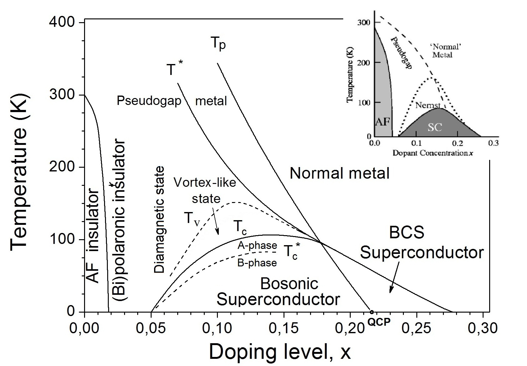
Figure 43: Genuine phase diagram of Bi-2212 showing various characteristic temperatures, $T_{p}$ (the pseudogap phase boundary ending at the polaronic QCP), $T^{*}$ (the BCS-like pseudogap formation temperature), $T_{v}$ (the onset of vortex-like excitations above the bulk superconducting transition temperature $T_{c}$) and $T^{*}_{c}$ (the onset of the first-order phase transition between the superconducting A and B phases), is compared with the other phase diagram 35 (see inset). The onset temperature of vortex formation $T_{v}$ is higher than $T_{c}$ but lower than the onset temperature $T^{*}$ of diamagnetism in the pseudogap state. The cuprate superconductor Bi-2212 undergoes a transition from the Fermi-liquid (BCS-type) superconducting state to the Bose-liquid superconducting state at the QCP ($x\simeq 0.22$) and this transition will be manifested as the normal metal-pseudogap metal transition when $H=H_{c2}$.

The values of $T_{c}$ in non-BCS cuprate superconductors are actually determined by low densities of bosons and only a small part of preformed Cooper pairs is involved in the superfluid Bose condensation. In 3D systems, the density of condensing (attracting) bosons is related to $n$ as $\rho_{B}=f_{s}n<<n$, where $f_{s}$ is the fraction of superfluid bosons. According to equations (VIII.8) and (213), $T_{c}$ first increases nearly as $T_{c}\sim(f_{s}n_{a}x)^{2/3}$ (in the 3D case) and $T_{c}\sim(f^{2D}_{s}n_{a}x)$ (in the 2D case), then reaches the maximum at optimal doping and exhibits the saturating or decreasing tendency with increase of $x$ and $m^{*}_{B}$. Thus, both curves $T^{3D}_{c}$ and $T^{2D}_{c}$ have a dome-like shape. A general advantage of quasi-2D versus 3D systems predicted by the superfluid Bose-liquid model is that superconductivity can be observed in a wider region of the phase diagram in the former than in the latter. Another important finding is that the onset temperature of the first-order phase transition $T^{*}_{c}$ separates two distinct superconducting phases of 3D Bose-type cuprate superconductors.

The entire phase diagram of Bi-2212 from Mott insulator to the heavily overdoped regime is shown in Fig. 43, where the characteristic temperatures $T^{*}_{c}$, $T_{c}$ and $T_{v}$ describe three distinct superconducting regimes, whereas two unusual metallic states exist below the crossover temperatures $T_{p}$ and $T^{*}$. The vortex-like state exists in the temperature range $T_{c}<T<T_{v}$, while the diamagnetic state persists up to the BCS-like pseudogap formation temperature $T^{*}$.

VIII.12 B. Unconventional Bose-liquid superconductivity and superfluidity in other systems

So far, the ideas of the BCS-like theory of superconductivity in simple metals based on the Cooper pairing of electrons is widely applied in various types of unconventional superconductors and superfluids. However, the mechanisms of unconventional superconductivity and superfluidity in other systems might be different from the BCS condensation of fermionic Cooper pairs. In this connection, we briefly discuss the underlying mechanisms of the unconventional superconductivity and superfluidity in other systems, in which the genuine superconducting/superfluid states arise at the pair and single particle condensations of attracting composite bosons (Cooper pairs and ⁴He atoms). We analyze the existing experimental data and explain the origins of the genuine superconducting/superfluid states and properties of other exotic matters using the theory of 3D and 2D Bose superfluids.

VIII.13 1. Novel superconducting states and properties of other exotic systems

There is much experimental evidence that the unconventional superconductivity in other systems (e.g., in organic and heavy-fermion compounds and ruthenate $\rm{Sr_{2}RuO_{4}}$) are actually similar to that in high-$T_{c}$ cuprates 17 ; 24 ; 28 ; 30 . Therefore, the above microscopic theory of superfluid Bose-liquids may provide a new insight into the physics of these unconventional superconductors. Actually, the electronic specific heat $C_{e}(T)$ of organic and heavy-fermion superconductors near $T_{c}$ has a striking resemblance with the $\lambda$-like specific heat anomaly in high-$T_{c}$ cuprates 30 ; 262 . Such a specific heat anomaly in unconventional organic and heavy-fermion superconductors can be explained by the law $C_{e}(T)\sim(T-T_{c})^{-1/2}$ similarly as in high-$T_{c}$ cuprates, whereas the second anomaly in the specific heat of heavy-fermion systems observed near $T_{c}^{*}$ somewhat below $T_{c}$ (see Refs. 27 ; 29 ) is also fairly explained by the law $C_{e}(T)\sim(T_{c}^{*}-T)^{-1/2}$. Experimental observations show 28 ; 263 ; 264 ; 265 ; 266 that the specific heat and London penetration depth in organic and heavy-fermion superconductors exhibit the power-law temperature dependences (i.e. $C_{e}(T)\sim T^{2}$, $T^{3}$ and $\lambda_{L}(T)\sim T^{2}$, $T^{3}$), which can be explained by the absence or smallness of the energy gap $\Delta_{g}$ in the excitation spectrum of 3D and 2D superfluid Bose liquids of Cooper pairs at low temperatures. Further, anomalous temperature dependences of the lower and upper critical magnetic fields were observed in these superconductors just like in high-$T_{c}$ cuprates near $T_{c}^{*}$ where the lower critical magnetic field $H_{c1}(T)$ suddenly increases (see Ref. 27 ) and the upper critical magnetic field $H_{c2}(T)$ has the upward curvature and a kink 28 ; 29 . We argue that the kink-like features in $H_{c1}(T)$ and $H_{c2}(T)$ observed in heavy-fermion superconductors are best described by the theory of a 3D superfluid Bose-liquid of unconventional Cooper pairs and intimately related to the kink-like feature of the superconducting order parameter $\Delta_{SC}(=\Delta_{B})$ near $T_{c}^{*}$ where the first-order phase transition between two distinct superconducting A and B phases occurs. Apparently, a first-order phase transition and a kink in $H_{c1}(T)$ were observed in heavy-fermion superconductors at a temperature $T^{*}_{c}$ lower than $T_{c}$ 27 ; 29 . Most importantly, a peak in the specific heat of these superconductors was also observed at the same temperature $T_{c}^{*}$ (see Ref. 27 ).

Interestingly, the temperature dependence of the London penetration depth $\lambda_{L}$ of organic and heavy-fermion superconductors has a close resemblance with that of $\lambda_{L}$ in high-$T_{c}$ cuprates. For example, the change in slope of $[\lambda_{L}(0)/\lambda_{L}(T)]^{2}$ observed near $T^{*}_{c}\simeq 0.7T_{c}$ in organic superconductor $(BEDT-TTF)_{2}$ $Cu(NCS)_{2}$ (see Fig. 4 in Ref. 263 ) is similar to the change in slope of $[\lambda_{L}(0)/\lambda_{L}(T)]^{2}$ in YBCO film shown in Fig. 39. While the change in slope of $\lambda_{L}^{-2}(T)$ observed near $T^{*}_{c}=0.2$K in heavy-fermion superconductor Upt₃ (see, Fig. 32 in Ref. 29 ) closely resembles that found in the above-mentioned YBCO film. According to the theory of Bose-liquid superconductivity, the first-order phase transition between A and B phases occurring near $T^{*}_{c}$ is accompanied by the change in slope of $[\lambda_{L}(0)/\lambda_{L}(T)]^{2}$ and $\lambda_{L}^{-2}(T)$ observed in the above organic and heavy-fermion superconductors.

Many researchers have attempted to explain the origins of the superconducting A and B phases in heavy-fermion systems in terms of the different BCS-like pairing theories. However, such an explanation of these superconducting phases seems to be inadequate and misleading. As discussed above, the superfluid single particle and pair condensates of bosonic Cooper pairs might be two distinct superconducting A and B phases in heave-fermion systems. Moreover, the origins of the gapless superconductivity and gapless excitations in these superconductors have also been poorly interpreted as the evidence for the existence of the nodes of BCS-like gaps. We argue that these distinctive superconducting properties of heavy-fermion systems are intimately related to the gapless excitation spectrum of a 3D superfluid Bose condensate of unconventional Cooper pairs, while the point or line nodes of the BCS-like gaps discussed in the current literature do not have direct relation to the heavy-fermion superconductivity.

Next we discuss the similarities of heavy-fermion and cuprate superconductors above the bulk superconducting transition temperature $T_{c}$. Experiments on heavy-fermion superconductors $\rm{CeRhIn_{5}}$, $\rm{CeCoIn_{5}}$ and $\rm{CeIrIn_{5}}$ (see Ref. 267 ) indicate the existence of a vortex-like state above $T_{c}$ that is reminiscent of the vortex-like state observed in cuprates above $T_{c}$. First the signs of remnant superconductivities were observed experimentally in $\rm{CeRhIn_{5}}$ and $\rm{CeCoIn_{5}}$ well above the bulk $T_{c}$ and then recent experiments have provided evidence for the existence of vortex-like excitations well above $T_{c}$ in $\rm{CeIrIn_{5}}$ 267 . These experimental findings suggest that the remnant superconductivity driven by pair condensation of bosonic Cooper pairs persists in the 3D-to-2D crossover region near surfaces or grain boundaries far above the bulk $T_{c}$. Therefore, the vortex-like excitations observed in $\rm{CeIrIn_{5}}$ (with $T_{c}=1.38$K) just like in high-$T_{c}$ cuprates would persist up to superconducting transition temperature $T_{c}^{2D}=T_{v}\simeq 4$K at quasi-2D surfaces or grain boundaries.

Finally, experimental results on unconventional superconductivity confirm clearly 268 that the novel superconducting phenomena in the layered ruthenate $\rm{Sr_{2}RuO_{4}}$ are actually similar to such phenomena in high-$T_{c}$ cuprates and to the phenomenon of superfluidity in ³He. One of the novel phenomena expected in the superconducting state of $\rm{Sr_{2}RuO_{4}}$ is emergence of the half-quantum vortices associated with the magnetic flux just half of the flux quantum $\Phi_{0}=h/2e$. The observations of such half-quantum vortices by Jang et al. 269 certainly give additional strong confirmation of the novel Bose-liquid superconductivity realized in $\rm{Sr_{2}RuO_{4}}$.

VIII.14 2. Superfluid Bose-liquid states and properties of liquid ³He and atomic Fermi gases

The BCS-like pairing theories describe fairly good the formation of unconventional Cooper pairs in liquid ³He, but fail to explain the genuine superfluidity in this system. We argue that these theories cannot explain the observed superfluid properties of ³He both at $T_{c}$ and below $T_{c}$. Actually, close examination of specific heat data shows that the observed behavior of the specific heat in liquid ³He near $T_{c}$ (see Fig. 19a in Ref. 198 ) contrasts with the step-like anomaly in conventional BCS superconductors and closely resembles a $\lambda$-like anomaly in $C_{e}(T)$ observed in high-$T_{c}$ cuprates. According to the theory of a 3D superfluid Bose-liquid of Cooper pairs, the specific heat of such a Bose-liquid diverges as $C(T)\sim(T-T_{c})^{1/2}$ near $T_{c}$ and will exhibit a $\lambda$-like anomaly at $T_{c}$, as observed in superfluid ³He 198 . Further, the first-order transition between the A- and B- phases of liquid ³He has been observed in the superfluid state below $T_{c}$ 32 and such a first-order phase transition at $T=T_{AB}$ is not also expected in BCS-like pairing theories. The mass of noninteracting bosonic Cooper pairs in liquid ³He is given by $m_{B}=2m^{*}_{3}$, where $m^{*}_{3}$ is the effective mass of ³He atoms. The superfluid transition temperature $T_{c}$ of liquid ³He can be determined from the relation

$$T_{c}=T^{*}_{BEC}\left[1+c_{0}\gamma_{B}\sqrt{\sqrt{2}k_{B}T^{*}_{BEC}/\xi_{BA}}\right],$$ (218)

where $T^{*}_{BEC}=3.31\hbar^{2}\rho^{2/3}_{B}/k_{B}m^{*}_{B}$.

The mass of the interacting bosonic Cooper pairs $m^{*}_{B}$ is determined from Eq. (181) and larger than $2m^{*}_{3}$. The value of $T_{c}$ observed in liquid ³He can be obtained by assuming that only a small attractive part of a Bose gas of Cooper pairs would condense into a superfluid Bose-liquid state at $T_{c}$ and the respective BEC temperature of such a small part of bosonic Cooper pairs is lower than $T_{c}$. In order to estimate $T^{*}_{BEC}$, we take $\rho_{B}=1.14\cdot 10^{19}\rm{cm^{-3}}$ $m^{*}_{B}=1.2m_{B}=2.4m^{*}_{3}$ and $m^{*}_{3}=5.5m_{3}$ 198 . Then we obtain $T^{*}_{BEC}=2.242\cdot 10^{-3}$K. If we assume $\gamma_{B}=0.4$ and $k_{B}T^{*}_{BEC}/\xi_{BA}=0.1$, we find $T_{c}\simeq 2.72\cdot 10^{-3}$K which is in good agreement with the observed value of $T_{c}=2.7\cdot 10^{-3}$K in liquid ³He.

The first-order phase transition between the A and B phases of liquid ³He occurs without any doubt at $T^{*}_{c}=T_{AB}$ and these superfluid A and B phases are roughly characterized by the half-integer $h/4m^{*}_{3}$ (at $T>T^{*}_{c}$) and integer $h/2m^{*}_{3}$ (at $T\leq T^{*}_{c}$) flux quantizations. The signs of the existence of half flux quanta in the superfluid ³He-A were discussed in Ref. 271 . Based on the above results, we discuss the microscopic origin of the half-quantum vortices in the bulk of superfluid ³He-$A$ and clarify why such vortices had not been clearly detected for a long time. The energy gap characterizing the formation of the paired state of two bosons (Cooper pairs) opens in the excitation spectrum of a 3D superfluid Bose condensate at $T>T_{c}^{*}=T_{AB}$ and increases with increasing temperature towards $T_{c}$. This gap $\Delta_{g}(T)=\sqrt{\tilde{\mu}_{B}^{2}(T)-\Delta_{B}^{2}(T)}$ is vanishingly small at temperatures close to the $AB$ phase boundary but the energy gap $\Delta_{g}(T\lesssim T_{c})\simeq\tilde{\mu}_{B}$ near $T_{c}$ is much more larger than the gap $\Delta_{g}(T\gtrsim T_{AB})\gtrsim 0$ near $T_{AB}$, i.e., at temperatures close to $T_{AB}$ and $T_{c}$ the situations for paired bosonic Cooper pairs, which behave like superfluid entities with mass $2m^{*}_{B}\sim 4m^{*}_{3}$, are completely different. It follows that the half-quantum vortices in the $A$ phase of the bulk superfluid ³He is much better manifested at temperatures close to $T_{c}$ than at lower temperatures, since the half-quantum vortices would be stabilized at higher temperatures close to $T_{c}$, but not at lower temperatures close to the $AB$ phase boundary. Further, the thermal dissociation of some part of boson pairs occurs in the temperature range $T_{AB}<T<T_{c}$ and the full-quantum vortices with circulation $h/m^{*}_{B}\sim h/2m^{*}_{3}$ can be also expected in ³He-$A$. Therefore, the full-quantum vortices tend to coexist with half-quantum vortices even near $T_{c}$. Apparently, this picture is consistent with a recent experimental result (see Ref. 271 ), in which the measurement was performed near $T_{c}$ and the coexistence of full- and half- quantum vortices in the bulk $A$ phase of superfluid ³He has inevitably occurred. The half-quantum vortices in superfluid ³He-$A$ phase are associated with the excitations of pair condensates of bosonic Cooper pairs rather than other effects. The nucleation process of the $B$-phase of superfluid ³He at $T=T_{AB}$ 32 is associated with the onset of the single particle condensation of bosonic Cooper pairs at $T=T^{*}_{c}=T_{AB}$.

The above-mentioned first-order phase transition between the A and B phases of liquid ³He is accompanied by both an abrupt jump-like increase of the critical velocity $v_{c}(T)=\sqrt{\Delta_{B}(T)/m_{B}}$ three times and a similar abrupt increase of the superfluid density, which have been observed in superfluid ³He at $T\simeq(0.6-0.7)T_{c}$ 270 . Clearly, the sharp increase of $\Delta_{B}(T)$ at the vanishing of the gap $\Delta_{g}$ in $E_{B}(k)$ near $T_{c}^{*}$ leads to the jump-like increasing of $v_{c}(T)$ and superfluid density $\rho_{s}(T)$ at $T\leq T_{c}^{*}$.

The unconventional superfluidity was also observed in ultracold atomic Fermi gases with an extremely high transition temperature with respect to the Fermi temperature near $T/T_{F}=0.2$ and this novel superfluidity in atomic Fermi gases occurs also in the limit of strong interactions and defies a conventional BCS description, as reported in Ref. 26 . We argue that the onset of Cooper pairing and superfluidity in these systems can occur at different temperatures ($T=T^{*}$ and $T=T_{c}<T^{*}$), since the atomic Fermi gas system like high-$T_{c}$ cuprates retains some of the characteristics of the pseudogap phase such as a BCS-like dispersion and a partially gapped density of states above $T_{c}$, but they does not exhibit superfluidity 26 . Therefore, the novel Bose-liquid superfluidity can be realized in ultracold atomic Fermi gases only below $T_{c}$, where the existence of the single particle and pair condensates of bosonic Cooper pairs as the superfluid $B$ and $A$ phases is quite possible similarly as in liquid ³He.

VIII.15 3. Superfluid Bose-liquid states and properties of liquid ⁴He

We now discuss the validity of the microscopic theory of Bose-liquid superfluidity in liquid ⁴He. The mass density of liquid ⁴He is $0.145g/\rm{cm}^{3}$ 30 and the total density of ⁴He atoms is $2.17\cdot 10^{22}\rm{cm^{-3}}$. As is well-known, the experimentally measured value of the $\lambda$-transition temperature $T_{\lambda}$ in liquid ⁴He is equal to 2.17 K 30 , which is lower than the BEC temperature $T_{BEC}\simeq 3.11$ K determined by using the mass of the free ⁴He atoms $(m_{4}=6.68\cdot 10^{-24}g)$ and assuming that all atoms of liquid ⁴He undergo a BEC. However, the liquid ⁴He is the strongly interacting Bose system where the effective mass $m^{*}_{4}$ of ⁴He atoms is determined from Eq. (181). Further, only an attractive part (perhaps about half) of ⁴He atoms can undergo a superfluid condensation. The superfluid transition temperature $T_{\lambda}$ in liquid ⁴He can be roughly estimated using Eq. (218). By taking $\rho_{B}=1.36\cdot 10^{22}\rm{cm^{-3}}$, $\rho_{B}\tilde{V}_{B}/\xi_{BR}=0.38$ and $m^{*}_{B}=m^{*}_{4}\simeq 1.611m_{4}$ for liquid ⁴He, we find $T^{*}_{BEC}\simeq 1.413$ K. If we assume that $\gamma_{B}=1$ and $k_{B}T^{*}_{BEC}/\xi_{BA}=0.1$ for superfluid ⁴He, we see that $T_{\lambda}\simeq 2.17$ K, thus providing an explanation of the observed value of $T_{\lambda}=2.17$ K.

According to the above microscopic theory of superfluid Bose-liquid, the specific heat of superfluid ⁴He, diverges as $C_{v}(T)\sim(T_{\lambda}-T)^{-1/2}$ and exhibits a clear $\lambda$-like anomaly at $T_{\lambda}$. The excitation spectrum $E_{B}(k)$ of this Bose superfluid becomes gapless and phonon-like in the temperature range $0\leq T\leq T^{*}_{c}$ below $T_{\lambda}$. The energy gap $\Delta_{g}$ appearing in $E_{B}(k)$ at the pair condensation of attracting bosons (⁴He atoms) above $T^{*}_{c}$ is responsible for the deviation of the specific heat $C_{v}(T)$ from the phonon-like $T^{3}$ law 214 and for the half-integer circulation quantum $h/2m^{*}_{4}$ 212 observed in superfluid ⁴He. Such a gap in the excitation spectrum of superfluid ⁴He at zero-momentum state is evidently absent and was not observed (see Ref. 214 ). This is a characteristic signature of the single particle condensation of attracting ⁴He atoms. Actually, depletion of the single particle condensate ($n_{B0}\neq 0$) at $T\leq T^{*}_{c}$ as a function of $\gamma_{B}$ (Fig. 26) and temperature (Fig. 30), as well as its absence ($n_{B0}=0$) in the temperature range $T^{*}_{c}<T<T_{\lambda}$ are in fair agreement with the experimental data available for liquid ⁴He 215 ; 216 . Experiments indicate (see 214 ; 215 ) that the condensate fraction is very small ($n_{B0}\simeq(1.8\pm 10)\%$ at $T=1.2$ K and $n_{B0}\simeq 10\%$ at $T=0$) and the temperature-dependent $n_{B0}(T)$ has a feature manifesting in a marked (several times) increase of $n_{B0}$ below $T\sim 1$ K. This feature of $n_{B0}(T)$ observed in superfluid ⁴He is indicative of the appearance of the energy gap in the excitation spectrum of this superfluid at $T=T^{*}_{c}\gtrsim 1.2$ K. Apparently, the interatomic interaction in liquid ³He is relatively weaker than such an interaction in ⁴He. Therefore, the condensate fraction in superfluid ³He must be larger than in superfluid ⁴He. Indeed, the condensate fraction in liquid ³He-⁴He mixtures was found to be $n_{B0}\simeq 0.18$ 272 much larger than $n_{B0}\simeq 0.10$ in liquid ⁴He 215 . The single particle and pair condensations of attracting bosons are responsible for the integer ($h/m^{*}_{4}$) and half-integer ($h/2m^{*}_{4}$) flux quantizations in superfluid ⁴He, where two distinct pair and single particle condensates of such bosons can also exist as the two distinct superfluid A and B phases in the temperature ranges $T^{*}_{c}<T<T_{\lambda}$ and $0\leq T\leq T^{*}_{c}$, respectively. The first signs of the half-integer $h/2m^{*}_{4}$ flux quantization in superfluid ⁴He was actually observed by Whitmore and Zimmerman 212 and other authors 213 .

Next we turn to the superfluid critical velocity in liquid ⁴He. The helium critical velocities of 60-70 m/s, predicted by the Landau criterion for superfluidity, are much (two orders of magnitude) larger than measured velocities of superfluid flow 273 . Experiments yield values for the helium critical velocity in the range of 1 cm/s to 1 m/s, depending on the particular geometry 30 ; 273 . The existence of superfluidity in liquid ⁴He can be understood in terms of two different critical velocities 274 . For velocities smaller than the upper critical velocity $v_{c2}$ (which is very well approximated by the Landau critical velocity defined by us as $v_{c2}=v_{L}=\sqrt{\Delta_{B}/m^{*}_{4}}$), there is no creation of phonon-like excitations. The breakdown of superfluidity is caused by these excitations and superfluidity is completely destroyed at $v>v_{c2}$. While the source of partial destruction of superfluidity could be the creation of vortices, since the superfluid flow above the lower critical velocity $v_{c1}$, implying the existence of a second larger critical velocity $v_{c2}>>v_{c1}$, means the possibility of partial superfluidity for $v_{c1}<v<v_{c2}$. Essentially, the distinctive roles played by the lower and upper critical velocities $v_{c1}$ and $v_{c2}$ in superfluid ⁴He closely resemble such roles played by the lower and upper critical magnetic fields $H_{c1}$ and $H_{c2}$ in high-$T_{c}$ cuprates and other unconventional superconductors. We now estimate the lower critical velocity $v_{c1}=(\hbar/2m^{*}_{4}R_{0})ln(R_{0}/d)$ (where $R_{0}$ is the radius of a vortex ring, $d$ is the interatomic distance) 239 and the upper critical velocity $v_{c2}=\sqrt{\Delta_{B}/m^{*}_{4}}$ in superfluid ⁴He. One can assume that $R_{0}$ would be of the order of $10^{-6}cm$ 275 , while $d$ is of order $4{\AA}$ 276 . If we take $R_{0}=4\cdot 10^{-6}$ cm, we obtain $v_{c1}=56$ cm/s which is consistent with the experimental data 30 ; 273 . Assuming that the superfluid order parameter $\Delta_{B}$ is of order $k_{B}T_{\lambda}$ we find that the upper critical velocity $v_{c2}=65.4$ m/s above which the creation of phonon-like excitations leads to the breakdown of superfluidity in liquid ⁴He.

Finally, the observed low temperature heat capacity $C_{v}(T)\sim T^{2}$ of 2D superfluid ⁴He in mesopores 277 is also consistent with the prediction of the theory of a 2D superfluid Bose-liquid. Whereas the shift of the superfluid frequency observed there (with the anomaly at $T\simeq(0.7-0.8)T_{C}$) as a function of the temperature closely resembles the kink-like behavior of the order parameter $\Delta_{B}$ of a 3D superfluid Bose-liquid. Perhaps the ⁴He adatoms in mesopores manifest both 2D- and 3D-superfluidity one of them will display in the heat capacity and another will display in the superfluid frequency shifts. Further, the new vortex topology in thin ⁴He superfluid film on porous media might be intermediate between the bulk superfluid liquid and flat superfluid film configuration, as discussed in Ref. 278 . This vortex-like state existing at temperatures $T_{\lambda}<T<T_{c}^{2D}$ can also be interpreted as a result of the crossover from 3D to 2D nature of the superfluid state and formation of 3D vortices at the destruction of the bulk superfluidity in the 3D-to-2D crossover region (i.e., in thin ⁴He film on porous substrate).

IX IX. New criteria and principles for unconventional superconductivity and superfluidity

From the above considerations, it is clear to anyone by now that the high-$T_{c}$ cuprates and other related systems (e.g. organic and heavy-fermion systems, ruthenate $\rm{Sr_{2}RuO_{4}}$, superfluid ³He and atomic Fermi gases) with low Fermi energies cannot be BCS-type superconductors and superfluids. Therefore, most researchers at last should realize this fact and know that the underlying mechanisms of novel (unconventional) superconductivity and superfluidity can be fundamentally different from the often discussed currently $s$-, $p$- or $d$-wave BCS-type (Fermi-liquid) superconductivity and superfluidity. While they should know new criteria and principles of unconventional superconductivity (or superfluidity) that incorporate also the BCS-type superconductivity as a particular case. We are now in position to formulate such criteria and principles, which are valid for various superconductors and superfluids, as follows:

(1) The BCS-type superconductivity and superfluidity occur, as a rule, in weakly interacting Fermi systems (e.g., in conventional metals, heavily overdoped cuprates and other systems), in which the Fermi energy is large enough $\varepsilon_{F}>2\varepsilon_{A}$ (or $\varepsilon_{F}>>\Delta_{F}$) and the Cooper pairs have fermionic nature

(2) In conventional superconductors/superfluids, the onset temperature of Cooper pairing $T^{*}$ coincides with $T_{c}$ and the formation of a BCS pairing gap $\Delta_{F}$ on the Fermi surface at $T_{c}$ is a criterion for the occurrence of superconductivity (or superfluidity)

(3) The BCS-type Cooper pairing is a necessary, but not a sufficient for the occurrence of unconventional superconductivity and superfluidity

(4) Unconventional superconductivity and superfluidity in exotic matters (e.g. in high-$T_{c}$ cuprates, heavy-fermion and organic compounds, $\rm{Sr_{2}RuO_{4}}$, liquid ³He and atomic Fermi gases), as a rule, require both the Cooper pairing of fermions and the bosonization of Cooper pairs.

(5) The high-$T_{c}$ cuprates and other related systems having the small Fermi energies ($\varepsilon_{F}<2\varepsilon_{A}$) and exhibiting the pseudogap behaviors above $T_{c}$ are in bosonic limit of Cooper pairs, and therefore, they are unconventional (bosonic) superconductors and superfluids.

(6) The mechanism of unconventional Cooper pairing and the mechanism of the condensation of non-overlapping Cooper pairs into the superconducting/superfluid Bose-liquid state are fundamentally different.

(7) In pseudogap systems, as a rule, the formation of bosonic Cooper pairs occurs first at a temperature $T^{*}$ above $T_{c}$ and then such Cooper pairs begin to condense into a Bose superfluid at a $\lambda$-like transition temperature $T_{c}$.

(8) The criteria for bosonization of Cooper pairs (the conditions (99) and (106)), the appearance of the coherence parameter $\Delta_{B}$ of bosonic Cooper pairs at $T_{c}$ and the coexistence of the BCS-like fermionic order parameter $\Delta_{F}$ and the superfluid Bose condensate order parameter $\Delta_{B}$ below $T_{c}$ are the new criteria for the occurrence of unconventional superconductivity and superfluidity.

(9) In Bose systems the following universal law of superfluid condensation of attracting bosons would hold: the pair condensation of such bosons occurs first at $T_{c}$ and then their single particle condensation sets in at a lower temperature $T_{c}^{*}$ than the $T_{c}$.

(10) In bosonic superconductors/superfluids, as a rule, a $\lambda$-like second-order phase transition will occur first at $T_{c}$ and then a first-order phase transition occurs somewhat below $T_{c}$ or even far below $T_{c}$, while the pair and single particle condensations of attracting bosons (unconventional Cooper pairs and ⁴He atoms) result in the formation of two distinct superconducting/superfluid A and B phases below $T_{c}$ similarly in superfluid ³He.

(11) Only a small attractive part of a Bose gas of Cooper pairs condenses into a Bose superfluid at $T_{c}$. Similarly, a certain attractive part of atoms in liquid ⁴He condenses into a Bose superfluid at $T_{\lambda}$.

X X. CONCLUSIONS

In this work, we have elaborated a consistent, predictive and empirically adequate microscopic theory of pseudogap phenomena and unconventional Bose-liquid superconductivity and superfluidity in high-$T_{c}$ cuprates and other systems with low Fermi energies. This theory based on the radically new and conceptually more consistent approaches enabled us to describe properly the pseudogap phenomena and the unconventional superconductivity and superfluidity in various substances.

Now we conclude by summarizing the above theoretical results and the key physical features that distinguish unconventional superconductors and superfluids from the conventional BCS superconductors (superfluid Fermi liquids). This can serve as a quide for discriminating between superconducting/superfluid systems that have usual BCS behavior and those which cannot be consistently explained by the BCS-like ($s$-, $p$- or $d$-wave) pairing theory. From the above considerations and experimental evidences, it follows that in BCS-type superconductors (i.e. in conventional metals and heavily overdoped cuprates) characterized by weak electron-phonon coupling, the charge carriers are quasi-free electrons or holes and strongly overlapping Cooper pairs, which condense into a superfluid Fermi-liquid state at $T_{c}$. In contrast, the high-$T_{c}$ cuprates falling between weak and strong electron-phonon coupling regimes are characterized by the pseudogap and non-overlapping bosonic Cooper pairs, which exist above $T_{c}$ and condense into a superfluid Bose-liquid state at $T_{c}$. In these polar materials the relevant charge carriers are polarons which are bound into bipolarons (at low dopings) and polaronic Cooper pairs (at intermediate dopings). The unconventional electron-phonon coupling and polaronic effects are more relevant to the underdoped, optimally doped and moderately overdoped cuprates than other factors and control the new physics of these high-$T_{c}$ materials. The mechanisms for the formation of the two types of pseudogaps observed in doped high-$T_{c}$ cuprates above $T_{c}$ and not encountered before in conventional superconductors are intimately related to the unconventional electron-phonon interactions. Specifically, the so-called non-pairing and pairing pseudogaps are induced by the polaronic effect and the BCS-like pairing of large polarons above $T_{c}$ in various high-$T_{c}$ cuprates, from the underdoped to the overdoped regime.

Our results provide a consistent picture of the microscopic origin of the two different pseudogap regimes and their respective crossover temperatures ($T_{p}$ and $T^{*}$) in the normal state of underdoped to overdoped cuprates. The polaronic pseudogap phase boundary ends at a specific QCP ($x_{p}=x_{QCP}\simeq 0.20-0.22$) and controls the new physics of high-$T_{c}$ cuprates in a wide region of temperatures and dopant concentration. This upper pseudogap crossover temperature $T_{p}$ characterizes the Fermi surface reconstruction (any large Fermi surface existing above $T_{p}$ transforms into a small polaronic Fermi surface below $T_{p}$). Actually, such a Fermi surface reconstruction occurring at a QCP predicted first theoretically 62 was observed experimentally much later 113 ; 114 . Another new physics is that the BCS-type Cooper pairing of polaronic carriers occurs at the lower pseudogap crossover temperature $T^{*}$, which is substantially greater than $T_{c}$ in the underdoped region and even in some optimally doped region and only approaches closely to $T_{c}$ and merges with the $T_{c}$ in the overdoped region of the phase diagram of high-$T_{c}$ cuprates. Two distinct pseudogaps have specific effects on the normal-state properties of underdoped to overdoped cuprates and manifest themeselves in the different anomalous behaviors of the temperature-dependent resistivity (e.g., a $T$-linear resistivity from $T_{p}$ down to $T^{*}$, anomalous resistive transitions at $T^{*}$, downward and upward deviations of the resistivity from $T$-linear law below $T^{*}$ and an abnormal resistivity peak between $T_{c}$ and $T^{*}$), in the asymmetric peaks and peak-dip-hump features of the tunneling spectra, in the jump-like specific heat anomalies above $T_{c}$ (i.e. at $T^{*}$) and in the novel isotope effects on $T^{*}$. Further, the pseudogap state described by the pertinent BCS-like pairing theory of fermionic quasiparticles would exist above $T_{c}$ in other unconventional superconductors and superfluids.

Most importantly, the bosonization of Cooper pairs and the unconventional superconductivity and superfluidity would occur in high-$T_{c}$ cuprates and other pseudogap systems. We have formulated the universal and more relevant criteria for bosonization of Cooper pairs in these systems using the uncertainty principle. We have found that the bosonization of Cooper pairs would occur in high-$T_{c}$ cuprates, heavy-fermion and organic compounds, liquid ³He, atomic Fermi gases and other systems under the conditions $\varepsilon_{F}\lesssim 2\varepsilon_{A}$ and $\Delta_{F}/\varepsilon_{F}\gtrsim 0.34\cdot(\varepsilon_{A}/\varepsilon_{F})^{1/3}$. The unconventional superconductivity and superfluidity occurring in the bosonic limit of Cooper pairs are expected in high-$T_{c}$ cuprates and other pseudogap systems where the superconductivity (superfluidity) is not simply caused by the formation of a BCS-like energy gap $\Delta_{F}$ on a Fermi surface. In these systems, the superconducting/superfluid transition at $T_{c}$ is more $\lambda$-like than the BCS or BEC transition and superconductivity (superfluidity) is not expected until the superfluid condensation temperature $T_{c}$ of the bosonic Cooper pairs is reached. In underdoped and overdoped cuprates, the bosonic Cooper pairs (with zero spin), the BCS-like gap $\Delta_{F}$ and related diamagnetic state exist below $T^{*}$, but high-$T_{c}$ superconductivity is only established when the part of such Cooper pairs condenses into a Bose superfluid at $T_{c}$. There is experimental evidence that the BCS-like fermionic excitation gap $\Delta_{F}$ exists as a pseudogap in high-$T_{c}$ cuprates 35 ; 228 ; 279 and other exotic superconductors 18 ; 24 ; 193 and atomic Fermi gases 26 . Actually, the BCS-like pairing of fermions at $T^{*}>T_{c}$ or $T^{*}>>T_{c}$ 21 ; 22 (cf. the pairing temperature $T_{p}=2T_{c}$ predicted in Ref. 64 ) may be considered as a first step toward a more complete treatment of novel Bose-liquid superconductivity and superfluidity in these pseudogap systems, where the BCS-like order parameter $\Delta_{F}$ should appear first above $T_{c}$, and then the BCS-like order parameter (or energy gap) $\Delta_{F}$ and the superfluid Bose condensate order parameter $\Delta_{B}$ (defining the boson superfluid stiffness) should coexist below $T_{c}$.

Our results clearly demonstrate that superconductivity(superfluidity) of bosonic Cooper pairs just like superfluidity of ⁴He atoms is well described by the mean field theory of attracting bosons and the superconducting/superfluid phase is identified with the coherence parameter $\Delta_{B}$ appearing below $T_{c}$. We have established the following law: the attractive Bose gases of Cooper pairs and ⁴He atoms undergo a $\lambda$-like superconducting/superfluid transition at $T_{c}$ (the onset temperature of pair condensation of bosons) and then a first-order phase transition at $T_{c}^{*}$ (the onset temperature of single particle condensation of bosons) lower than $T_{c}$ (in a 3D system) or at $T=0$ (in a 2D system). We have proved that the gapless superconductivity (superfluidity) occurs in 3D Bose systems below $T_{c}^{*}$ due to the vanishing of the energy gap $\Delta_{g}$ in $E_{B}(k)$ and this phenomenon in unconventional superconductors and superfluids is not caused by the point or line nodes of the BCS-like gap discussed in some $p$- and $d$-wave pairing models. We have discovered that the coherent single particle and pair condensates of bosonic Cooper pairs and ⁴He atoms exist as the two different superfluid A and B phases in high-$T_{c}$ cuprates and other unconventional superconductors and superfluids (e.g., ³He, ⁴He and atomic Fermi gases). According to the theory of a superfluid Bose-liquid, the cuprate high-$T_{c}$ superconductivity is more robust in quasi-two-dimensions than in three dimensions, i.e., $T_{c}$ is higher in quasi-2D than in 3D systems. Therefore, we see that three different superconducting phases exist in high-$T_{c}$ cuprates where the coherent pair condensate of bosonic Cooper pairs persists as the superconducting phase up to the temperature $T_{v}=T^{2D}_{c}>T^{3D}_{c}$ at quasi-2D grain boundaries and the coherent pair and single particle condensates of such composite bosons in 3D systems exist as the two distinct superconducting phases below $T_{c}=T_{c}^{3D}$. It follows that the persistence of the vortex-like excitations in high-$T_{c}$ cuprates above $T_{c}$ is caused by the destruction of the bulk superconductivity. The existence of such vortices is expected below the temperature $T_{v}$ lower than $T^{*}$ but higher than $T_{c}$. This means that diamagnetism and vortex formation above $T_{c}$ in high-$T_{c}$ cuprates are unrelated phenomena.

Clearly, the condensate and excitations of a Bose-liquid are unlike those of a BCS-like Fermi liquid. Therefore, not all the experimental methods are able to identify the true superconducting order parameter $\Delta_{SC}=\Delta_{B}$ in high-$T_{c}$ cuprates and other pseudogap systems. For example, the single-particle tunneling spectroscopy and ARPES provide information about the excitations gaps at the Fermi surface but fail to identify the true superconducting order parameter appearing below $T_{c}$ in bosonic superconductors. For this reason, a prolonged disput about the origin of unconventional superconductivity (i.e. superconducting other parameter) in the cuprates on the basis of tunneling and ARPES data has nothing to do with the underlying mechanism of high-$T_{c}$ cuprate superconductivity. The unconventional cuprate superconductivity is controlled by the coherence parameter (boson superfluid stiffness) $\Delta_{B}\sim\rho_{B}$ and only some selected experimental techniques can provide information about such a superconducting order parameter. In particular, the thermodynamic methods and the methods of critical current and magnetic field measurements are sensitive to the identification of $\Delta_{SC}(T)=\Delta_{B}(T)$ in unconventional superconductors.

We have convincingly demonstrated that many puzzling superconducting/superfluid properties of high-$T_{c}$ cuprates, heavy-fermion and organic compounds, $\rm{Sr_{2}RuO_{4}}$, quantum liquids (³He and ⁴He) and ultracold atomic Fermi gases observed experimentally are best described by the microscopic theory of the 3D Bose-liquid superconductivity and superfluidity. In particular, we have shown that the bulk superconductivity described by the theory of a 3D superfluid Bose-liquid provides a consistent picture of the highly unusual and intriguing superconducting properties (e.g., $\lambda$-like second-order phase transition at $T_{c}$, first-order phase transition and kink-like temperature dependences of superconducting parameters $\Delta_{SC}(T)$, $J_{c}(T)$, $H_{c1}(T)$, $H_{c2}(T)$, $\lambda_{L}(T)$ near $T_{c}^{*}$, gapless excitations and novel isotope effects on $T_{c}$) of high-$T_{c}$ cuprates. Experimental results confirming the occurrence of bulk superconductivity in the system $\rm{PrBa_{2}Cu_{3}O_{7-\delta}}$ 280 revitalizes the hypothesis that superconductivity originates also outside the cuprate-plane. Meanwhile, the grain boundary- and interface-related Bose-liquid superconductivity can persist up to room temperature in cuprate materials obtained under certain conditions.

Finally, we have formulated the new criteria and principles of unconventional superconductivity and superfluidity, which allow us to find the real applicability boundary (which up to now remains unknown) between BCS-type and Bose-type regimes of superconductivity and superfluidity in high-$T_{c}$ cuprates and other systems. The above theoretical predictions and their experimental confirmations speak strongly about in favor of the existence of novel superconducting/superfluid states, which arise in condensed matter systems at single particle and pair condensations of attracting bosonic Cooper pairs. Within the mean field theory of 3D and 2D superfluid Bose liquids, it is possible to describe the following unexplained features of high-$T_{c}$ cuprates and other superconductors and superfluids: (i) the novel features of the phase diagram of high-$T_{c}$ cuprates (e.g., vortex-like state existing in the temperature range $T_{c}<T<T_{v}$ and two distinct superconducting phases below $T_{c}$); (ii) the existence of a vortex-like state above $T_{c}$ and two distinct superconducting A and B phases in heavy-fermion systems below $T_{c}$; (iii) the existence of two distinct superfluid $A$ and $B$ phases in liquid ³He, (iv) the existence of first-order phase transitions in superfluid ³He (at $T=T_{AB}<T_{c}$), high-$T_{c}$ cuprates (at $T=T^{*}_{c}<T_{c}$) and heavy-fermion superconductors (at $T=T^{*}_{c}<T_{c}$) not expected in BCS-like pairing theories; (v) the underlying physics of superfluid ⁴He and the critical velocities of superfluid flow in ⁴He below $T_{\lambda}$; (vi) the deviation of the specific heat from the phonon-like $T^{3}$ dependence observed in superfluid ⁴He at about $T\gtrsim T^{*}_{c}\simeq 1$ K 214 ; (vii) the vortex-like state existing at temperatures $T_{\lambda}<T<T_{c}^{2D}$ in the crossover regime between the bulk superfluid liquid and thin ⁴He superfluid film; (viii) the unconventional superfluidity in ultracold atomic Fermi gases.

The above presented results may shed new light on unconventional mechanisms of superconductivity (superfluidity) in low-density nuclear systems-perhaps in the low-density nuclear matter in outer regions of nuclei and neutron stars.

Note added. After writing this work, I learned from report made by D.G. Gulyamova 281 that some characteristic signatures of room temperature superconductivity are seemingly observed in samples of Bi-based cuprates obtained at sun-furnace (in Tashkent) and containing coupled stacks of many quasi-2D superconducting layers. Experiments by Gulyamova’s group seem to give some evidence for grain boundary- and interface-related room temperature cuprate superconductivity that we predict here.

XI APPENDIX A: Boltzmann transport equations for Fermi components of Cooper pairs and bosonic Cooper pairs

The Boltzmann transport equation for the excited Fermi components of Cooper pairs in the relaxation time approximation can be written as

$$f^{0}_{C}(k)-f_{C}(k)=\frac{\tau_{BCS}(k)}{\hbar}\vec{F}\frac{\partial f_{C}}{\partial{k}},$$ (A.1)

where $f^{0}_{C}(k)$ is the equilibrium Fermi distribution function, $\tau_{BCS}(k)$ is the relaxation time of the Fermi components of Cooper pairs in the BCS-like pseudogap regime, $\vec{F}$ is a force acting on a charge carrier in the crystal.

We consider the conductivity of hole carriers in the presence of the electric field applied in the $x$-direction. Then we can write Eq. (A1) as

$$f^{0}_{C}(k)-f_{C}(k)=\frac{\tau_{BCS}(k)}{\hbar}\vec{F_{x}}\frac{\partial f_{C}(k)}{\partial k_{x}}=$$

$$=\frac{\tau_{BCS}(k)}{\hbar}\vec{F_{x}}\frac{\partial f_{C}(k)}{\partial E}\frac{\partial E}{\partial k_{x}}=$$

$$=\frac{\tau_{BCS}(k)}{\hbar}\vec{F_{x}}\hbar V_{x}\frac{\partial f_{C}(k)}{\partial E},$$ (A.2)

where $E(k)=\sqrt{\xi^{2}(k)+\Delta^{2}_{F}}$, $\xi(k)=\varepsilon(k)-\varepsilon_{F}$, $\varepsilon(k)=\hbar^{2}(k^{2}_{x}+k^{2}_{y}+k^{2}_{z})/2m_{p}$, $V_{x}=\frac{1}{\hbar}\frac{\partial E_{x}}{\partial k_{x}}=v_{x}\frac{\xi}{E}$, $v_{x}=\hbar k_{x}/m_{p}$.

The density of the Fermi components of Cooper pairs is determined from the relation

$$n^{*}_{p}=2\sum_{k}u_{k}f_{C}(k)=2\sum_{k}\frac{1}{2}(1+\frac{\xi}{E})f_{C}(k)=$$

$$=\frac{1}{(2\pi^{3})}\int(1+\frac{\xi}{E})f_{C}(k)d^{3}k$$

Using Eqs. (XI) and (XI) the current density in the $x$-direction can be defined as

$$J^{*}_{x}=\frac{e}{(2\pi)^{3}}\int v_{x}(1+\frac{\xi}{E})f_{C}(k)d^{3}k=$$

$$=\frac{e}{(2\pi)^{3}}\int v_{x}(1+\frac{\xi}{E})f^{0}_{C}(k)d^{3}k-$$

$$-\frac{e}{(2\pi)^{3}}\int v^{2}_{x}\tau_{BCS}(k)F_{x}\frac{\xi}{E}(1+\frac{\xi}{E})\frac{\partial f_{C}(k)}{\partial E}d^{3}k,$$ (A.4)

where $\xi$ and $E$ are even functions of $k$, while $v_{x}f^{0}_{C}(k)$ is an odd function of $v_{x}$. Since integration with respect to $dk_{x}$ ranges from $-\infty$ to $+\infty$, the first term in Eq. (XI) becomes zero, and only the second term remains, resulting in (for $F_{x}=+eE_{x}$)

$$J^{*}_{x}=-\frac{e^{2}E_{x}}{8\pi^{3}}\int v^{2}_{x}\tau_{BCS}(k)\frac{\xi}{E}(1+\frac{\xi}{E})\frac{\partial f_{C}(k)}{\partial E}d^{3}k.$$

Similarly, the current density of bosonic Cooper pairs in the $x$-direction is given by (for $F_{x}=+2eE_{x}$)

$$J^{B}_{x}=\frac{2e}{(2\pi)^{3}}\int v_{x}[f^{0}_{B}(k)-\tau_{B}(k)v_{x}F_{x}\frac{\partial f_{B}}{\partial\varepsilon}]d^{3}k=$$

$$=-\frac{e^{2}E_{x}}{2\pi^{3}}\int v^{2}_{x}\tau_{B}(k)\frac{\partial f_{B}}{\partial\varepsilon}d^{3}k,$$

XII APPENDIX B: Calculation of the Basic Parameters of a Superfluid Bose-liquid for $T=0$

For the model potential (137), $\Delta_{B}(\vec{k})$ will be approximated as

$$\Delta_{B}(\vec{k})=\left\{\begin{array}[]{lll}\Delta_{B1}&\textrm{for}|\varepsilon(k)|,|\varepsilon(k^{\prime})|\leq\xi_{BA},\\ \Delta_{B2}&\textrm{for}\xi_{BA}<|\varepsilon(k)|,|\varepsilon(k^{\prime})|\leq\xi_{BR},\\ 0&\textrm{for}\varepsilon(k)\textrm{or}\varepsilon(k^{\prime})>\xi_{BR}.\end{array}\right.$$ (B.4)

Then Eqs. (VII.1) and (VII.1) at $T=0$ are reduced to the following equations:

$$\Delta_{B1}=-D_{B}(V_{BR}-V_{BA})\Delta_{B1}I_{A}-V_{B1}\Delta_{B2}I_{R},$$

$$\Delta_{B2}=-V_{BR}\Delta_{B1}I_{A}-V_{BR}\Delta_{B2}I_{R},$$ (B.6)

and

$$\chi_{B1}=(V_{BR}-V_{BA})\rho_{B1}+V_{BR}\rho_{B2},$$ (B.7)

where

$$I_{A}=D_{B}\int^{\xi_{BA}}_{0}\frac{\sqrt{\varepsilon}d\varepsilon}{2\sqrt{(\varepsilon+\tilde{\mu}_{B})^{2}-\Delta^{2}_{B1}}},$$ (B.8)

$$I_{R}=D_{B}\int^{\xi_{BR}}_{\xi_{BA}}\frac{\sqrt{\varepsilon}d\varepsilon}{2\sqrt{(\varepsilon+\tilde{\mu}_{B})^{2}-\Delta^{2}_{B2}}},$$ (B.9)

$\rho_{B1}=\frac{1}{\Omega}\sum^{k_{A}}_{k=0}n_{B}(\vec{k})$, $\rho_{B2}=\frac{1}{\Omega}\sum^{k_{R}}_{k=k_{A}}n_{B}(\vec{k})$, $n_{B}(\vec{k})=[\exp(E_{B}(\vec{k})/k_{B}T)-1]^{-1}$, $\xi_{BA}=\varepsilon(k_{A})$, $\xi_{BR}=\varepsilon(k_{R})$.

For 3D Bose systems, $D_{B}={m_{B}}^{3/2}/\sqrt{2}\pi^{2}\hbar^{3}$. From Eq. (B.6), we obtain

$$\tilde{V}_{B}I_{A}=[V_{BA}-V_{BR}(1+V_{BR}I_{R})^{-1}]I_{A}=1.$$ (B.10)

At $\xi_{BA}>>\tilde{\mu}_{B}$, $\Delta_{B2}$, we obtain from Eq. (B.9)

$$I_{R}\simeq D_{B}\int\limits_{\xi_{BA}}^{\xi_{BR}}\sqrt{\varepsilon}\frac{d\varepsilon}{2\varepsilon}=D_{B}\left[\sqrt{\xi_{BR}}-\sqrt{\xi_{BA}}\right]$$ (B.11)

and

$$I_{R}\simeq\frac{1}{2}\int^{\xi_{BR}}_{\xi_{BA}}\frac{d\varepsilon}{\varepsilon}=\frac{D_{B}}{2}\ln\frac{\xi_{BR}}{\xi_{BA}},$$ (B.12)

for 3D and 2D Bose systems, respectively.

We can assume that almost all Bose particles have energies smaller than $\xi_{BA}$ and $\rho_{B}\simeq\rho_{B1}$. Using Eq. (VII.1) the expression for $\rho_{B}$ can be written as

$$2\rho_{B}\simeq D_{B}\int\limits_{0}^{\xi_{BA}}\sqrt{\varepsilon}\left[\frac{\varepsilon+\tilde{\mu}_{B}}{\sqrt{(\varepsilon+\tilde{\mu}_{B})^{2}-\Delta_{B1}^{2}}}-1\right]d\varepsilon$$ (B.13)

At $\rho_{B2}<<\rho_{B1}$ the result of Eq. (B.7) allows us to determine the renormalized chemical potential as $\tilde{\mu}_{B}=-\mu_{B}+2\rho_{B}(V_{BR}-V_{BA})$. While Eq. (B.8) determines the coherence parameter $\Delta_{B}=\Delta_{B1}$. From Eq. (B.10) it follows that the model interboson interaction potential defined by Eq. (137) reduces to the following simple BCS-like potential:

$$V_{B}(\vec{k}-\vec{k^{\prime}})=\left\{\begin{array}[]{ll}\vspace{0.2cm}-\tilde{V}_{B},\\ \ \ 0,\end{array}\ \ \begin{array}[]{ll}\vspace{0.2cm}|\xi(k)|,|\xi(k^{\prime})|\leqslant\xi_{BA},\\ \vspace{0.2cm}\textrm{otherwise}\\ \end{array}\right.$$ (B.18)

For a 3D Bose system, we obtain from Eqs.(B.8) and (B.13)

$$\frac{1}{D_{B}\tilde{V}_{B}}=\sqrt{\xi_{BA}+2\tilde{\mu}_{B}}-\sqrt{2\tilde{\mu}_{B}}.$$

and

$$\frac{3\rho_{B}}{D_{B}}=\lim_{\xi_{BA}\rightarrow\infty}\sqrt{\xi_{BA}+2\tilde{\mu}_{B}}(\xi_{BA}-\tilde{\mu}_{B})+$$

$$+\tilde{\mu}_{B}\sqrt{2\tilde{\mu}_{B}}-\xi_{BA}^{3/2}\simeq\tilde{\mu}_{B}\sqrt{2\tilde{\mu}_{B}}.$$ (B.21)

Equation (XII) reduces to the relation (139) and then the substitution of Eq. (139) into Eq. (XII) gives the relation (140). Further, $2\rho_{B}/D_{B}=2.612\sqrt{\pi}(k_{B}T_{BEC})^{3/2}$ 226 and Eq. (141) follows from Eq. (XII). For $E_{B}(0)=0$, equations (VII.1)-(VII.1) can now be expressed as

$$\Delta_{B}(\vec{k})=-V_{B}(\vec{k})\rho_{B0}\frac{\Delta_{B}(0)}{|\Delta_{B}(0)|}-$$

$$-\frac{1}{\Omega}\sum_{k^{\prime}\neq 0}V_{B}(\vec{k}-\vec{k}^{\prime})\frac{\Delta_{B}(\vec{k}^{\prime})}{2E_{B}(\vec{k}^{\prime})}(1+2n_{B}(\vec{k}^{\prime})),$$ (B.22)

$$\rho_{B}=\rho_{B0}+\frac{1}{\Omega}\sum_{k\neq 0}n_{B}(\vec{k}),$$ (B.23)

$$\chi_{B}(\vec{k})=V_{B}(\vec{k})\rho_{B0}+\frac{1}{\Omega}\sum_{k^{\prime}\neq 0}V_{B}(\vec{k}-\vec{k}^{\prime})n_{B}(\vec{k}^{\prime}).$$

Replacing the summation in Eqs. (B.23) and (XII) by an integration and taking into account the approximation (B.18), we obtain

$$2(\rho_{B}-\rho_{B0})=D_{B}\int\limits_{0}^{\xi_{BA}}\sqrt{\varepsilon}\left[\frac{\varepsilon+\tilde{\mu}_{B}}{\sqrt{\varepsilon^{2}+2\tilde{\mu}_{B}}}-1\right]d\varepsilon,$$

$$\tilde{V}_{B}\rho_{B0}=\tilde{\mu}_{B}\left[1-\tilde{V}_{B}D_{B}\int\limits_{0}^{\xi_{BA}}\frac{\sqrt{\varepsilon}d\varepsilon}{2\sqrt{\varepsilon^{2}+2\tilde{\mu}_{B}\varepsilon}}\right].$$ (B.26)

From Eqs. (XII) and (B.26), we obtain Eqs. (143) and (VII.3), respectively. For 2D Bose systems, $D_{B}=m_{B}/2\pi\hbar^{2}$ and the multiplier $\sqrt{\varepsilon}$ under the integrals in Eqs. (XII) and (B.26) will be absent.

At $\gamma_{B}<\gamma^{*}_{B}$, evaluating the integrals in Eq. (VII.3) we have

$$W_{0}=D_{B}\Omega\Big{\{}\frac{2}{5}\Big{[}(\xi_{A}+2\Delta_{B})^{5/2})-\xi^{5/2}_{A}\Big{]}+$$

$$+\frac{4}{15}(2\Delta_{B})^{5/2}-\frac{2\Delta_{B}}{3}\xi^{3/2}_{A}-\frac{4\Delta_{B}}{3}(\xi_{A}+2\Delta_{B})^{3/2}-$$

$$-\Delta^{2}_{B}\Big{[}(\xi_{A}+2\Delta_{B})^{1/2}-(2\Delta_{B})^{1/2}\Big{]}\Big{\}},$$

.

In order to simplify Eq. (XII) further, we can expand the brackets $(\xi_{BA}+2\Delta_{B})^{5/2}$, $(\xi_{BA}+2\Delta_{B})^{3/2}$ and $(\xi_{BA}+2\Delta_{B})^{1/2}$ in this equation in powers of $2\Delta_{B}/\xi_{BA}$ as

$$(\xi_{BA}+2\Delta_{B})^{5/2}=\xi^{5/2}_{BA}\Big{(}1+\frac{2\Delta_{B}}{\xi_{BA}}\Big{)}^{5/2}\simeq$$

$$\simeq\xi^{5/2}_{BA}\Big{\{}1+\frac{5\Delta_{B}}{\xi_{BA}}+\frac{15}{2}\Big{(}\frac{\Delta_{B}}{\xi_{BA}}\Big{)}^{2}+\frac{5}{2}\Big{(}\frac{\Delta_{B}}{\xi_{BA}}\Big{)}^{3}...\Big{\}},$$

$$(\xi_{BA}+2\Delta_{B})^{3/2}=\xi^{3/2}_{BA}\Big{(}1+\frac{2\Delta_{B}}{\xi_{BA}}\Big{)}^{3/2}\simeq$$

$$\simeq\xi^{3/2}_{BA}\Big{\{}1+\frac{3\Delta_{B}}{\xi_{BA}}+\frac{3}{2}\Big{(}\frac{\Delta_{B}}{\xi_{BA}}\Big{)}^{2}-...\Big{\}},$$

$$(\xi_{BA}+2\Delta_{B})^{1/2}=\xi^{1/2}_{BA}\Big{(}1+\frac{2\Delta_{B}}{\xi_{BA}}\Big{)}^{1/2}\simeq$$

$$\simeq\xi^{1/2}_{BA}\Big{\{}1+\frac{\Delta_{B}}{\xi_{BA}}-...\Big{\}},$$

Substituting Eqs. (XII), (XII) and (XII) into Eq. (XII), we find

$$W_{0}=D_{B}\Omega\Big{\{}\frac{2}{5}\Big{[}\xi^{5/2}_{BA}+5\Delta_{B}\xi^{3/2}_{BA}+\frac{15}{2}\Delta^{2}_{B}\xi^{1/2}_{BA}+$$

$$+\frac{5}{2}\Delta^{3}_{B}/\xi^{1/2}_{BA}-\xi^{5/2}_{BA}\Big{]}-\frac{4}{15}(2\Delta_{B})^{5/2}-\frac{2\Delta_{B}}{3}\xi^{3/2}_{BA}-$$

$$-\frac{4\Delta_{B}}{3}\Big{[}\xi^{3/2}_{BA}+3\Delta_{B}\xi^{1/2}_{BA}+\frac{3}{2}\Delta^{2}_{B}/\xi^{1/2}_{BA}\Big{]}-\Delta^{2}_{B}\xi^{1/2}_{BA}-$$

$$-\Delta^{3}_{B}/\xi^{1/2}_{BA}+\Delta^{2}_{B}(2\Delta_{B})^{1/2}\Big{\}}=$$

$$=D_{B}\Omega\Big{\{}2\Delta_{B}\xi^{3/2}_{BA}-\frac{2\Delta_{B}}{3}\xi^{3/2}_{BA}-\frac{4\Delta_{B}}{3}\xi^{3/2}_{BA}+$$

$$+3\Delta^{2}_{B}\xi^{1/2}_{BA}-4\Delta^{2}_{B}\xi^{1/2}_{BA}+\Delta^{3}_{B}/\xi^{1/2}_{BA}-2\Delta^{3}_{B}/\xi^{1/2}_{BA}-$$

$$-\Delta^{2}_{B}\xi^{1/2}_{BA}-\Delta^{3}_{B}/\xi^{1/2}_{BA}-\frac{4}{15}(2\Delta_{B})^{5/2}+\Delta^{2}_{B}(2\Delta_{B})^{1/2}\Big{\}}=$$

$$=D_{B}\Omega\Big{\{}3\Delta^{2}_{B}\xi^{1/2}_{BA}-5\Delta^{2}_{B}\xi^{1/2}_{BA}-2\Delta^{3}_{B}/\xi^{1/2}_{BA}-\frac{\sqrt{2}}{15}\Delta^{5/2}_{B}\Big{\}}=$$

$$=D_{B}\Omega\Delta^{2}_{B}\xi^{1/2}_{BA}\Big{\{}-2-2\frac{\Delta_{B}}{\xi_{BA}}-\frac{\sqrt{2}}{15}\Big{(}\frac{\Delta_{B}}{\xi_{BA}}\Big{)}^{1/2}\Big{\}}.$$

At $\Delta_{B}/\xi_{BA}<<1$, we have

$$W_{0}\simeq-2D_{B}\Delta^{2}_{B}\xi^{1/2}_{BA}\Omega.$$ (B.32)

XIII APPENDIX C: Calculation of the Basic Parameters of a 3D Superfluid Bose-liquid for the temperature range $0<T\leq T_{c}$

Using the model potential (137), we can write Eqs. (VII.1) and (VII.1) as

$$\frac{2\rho_{B}}{D_{B}}=\int\limits_{0}^{\infty}\sqrt{\varepsilon}\left[\frac{(\varepsilon+\tilde{\mu}_{B})}{\sqrt{(\varepsilon+\tilde{\mu}_{B})^{2}-\Delta_{B}^{2}}}-1\right]d\varepsilon+$$

$$2\int\limits_{0}^{\infty}\frac{\sqrt{\varepsilon}(\varepsilon+\tilde{\mu}_{B})d\varepsilon}{\sqrt{(\varepsilon+\tilde{\mu}_{B})^{2}-\Delta_{B}^{2}}\left[\exp(\frac{\sqrt{(\varepsilon+\tilde{\mu}_{B})^{2}-\Delta_{B}^{2}}}{k_{B}T})-1\right]},$$ (C.1)

$$\frac{2}{D_{B}\tilde{V}_{B}}=\int\limits_{0}^{\xi_{BA}}\frac{\sqrt{\varepsilon}d\varepsilon}{\sqrt{(\varepsilon+\tilde{\mu}_{B})^{2}-\Delta_{B}^{2}}}+$$

$$2\int\limits_{0}^{\xi_{BA}}\frac{\sqrt{\varepsilon}d\varepsilon}{\sqrt{(\varepsilon+\tilde{\mu}_{B})^{2}-\Delta_{B}^{2}}\left[\exp(\frac{\sqrt{(\varepsilon+\tilde{\mu}_{B})^{2}-\Delta_{B}^{2}}}{k_{B}T})-1\right]}.$$

According to Eq. (XII) the first integral in Eq. (XIII) at $\tilde{\mu}_{B}=\Delta_{B}$ is equal to $2\tilde{\mu}_{B}\sqrt{2\tilde{\mu}_{B}}/3$. From Eq. (XII) it follows that the first integral in Eq. (XIII) at $\tilde{\mu}_{B}=\Delta_{B}$ is equal to $2[\sqrt{\xi_{BA}+2\tilde{\mu}_{B}}-\sqrt{2\tilde{\mu}_{B}}]$. The main contributions to the latter integrals in Eqs. (XIII) and (XIII) come from small values of $\varepsilon$, so that for $T<<T_{c}$ and $\tilde{\mu}_{B}=\Delta_{B}$ the latter integrals in Eqs. (XIII) and (XIII) can be evaluated approximately as

$$2\int\limits_{0}^{\infty}\frac{\sqrt{\varepsilon}(\varepsilon+\tilde{\mu}_{B})d\varepsilon}{\sqrt{\varepsilon^{2}+2\varepsilon\tilde{\mu}_{B}}\left[\exp\left[\sqrt{\frac{\varepsilon^{2}+2\varepsilon\tilde{\mu}_{B}}{k_{B}T}}\right]-1\right]}\approx$$

$$\approx\sqrt{2\tilde{\mu}_{B}}\int^{\infty}_{0}\frac{d\varepsilon}{\exp\left[\frac{\sqrt{2\varepsilon\tilde{\mu}_{B}}}{k_{B}T}\right]-1}=\frac{(\pi k_{B}T)^{2}}{3\sqrt{2\tilde{\mu}_{B}}},$$ (C.3)

$$2\int\limits_{0}^{\infty}\frac{\sqrt{\varepsilon}d\varepsilon}{\sqrt{\varepsilon^{2}+2\varepsilon\tilde{\mu}_{B}}\left[\exp\left[\frac{\sqrt{\varepsilon^{2}+2\varepsilon\tilde{\mu}_{B}}}{k_{B}T}\right]-1\right]}\approx$$

$$\approx\frac{2}{\sqrt{2\tilde{\mu}_{B}}}\int^{\infty}_{0}\frac{d\varepsilon}{\exp\left[\frac{\sqrt{2\varepsilon\tilde{\mu}_{B}}}{k_{B}T}\right]-1}=\frac{(\pi k_{B}T)^{2}}{3\sqrt{2}\tilde{\mu}_{B}^{3/2}}.$$ (C.4)

Further, according to Eqs. (XII) and (B.23), the term $2\rho_{B0}/D_{B}$ should be present in Eq. (XIII), while the term $2\rho_{B0}/\tilde{\mu}_{B}D_{B}$ would be present in Eq. (XIII). Thus, at $\tilde{\mu}_{B}=\Delta_{B}$ and $T<<T_{c}$, Eqs. (XIII) and (XIII) can now be written as

$$\frac{2\rho_{B}}{D_{B}}\simeq\frac{2\rho_{B0}(T)}{D_{B}}+\frac{(2\tilde{\mu}_{B})^{3/2}}{3}+\frac{(\pi k_{B}T)^{2}}{3\sqrt{2\tilde{\mu}_{B}}},$$ (C.5)

$$\frac{2\tilde{\mu}_{B}}{D_{B}\tilde{V}_{B}}\simeq\frac{2\rho_{B0}(T)}{D_{B}}+2\tilde{\mu}_{B}[\sqrt{\xi_{BA}+2\tilde{\mu}_{B}}-\sqrt{2\tilde{\mu}_{B}}]+$$

$$+\frac{(\pi k_{B}T)^{2}}{3\sqrt{2\tilde{\mu}_{B}}},$$ (C.6)

from which we obtain Eqs. (150) and (VII.4).

In the case of $\Delta_{g}\neq 0$ (or $\rho_{B0}=0$) and $\tilde{\mu}_{B}>>\Delta_{B}$, the first integral both in (XIII), and in (XIII) can be evaluated approximately using the Taylor expansion

$$\frac{1}{\sqrt{(\varepsilon+\tilde{\mu}_{B})^{2}-\Delta_{B}}}\simeq\frac{1}{\varepsilon+\tilde{\mu}_{B}}\left[1+\frac{\Delta^{2}_{B}}{2(\varepsilon+\tilde{\mu}_{B})^{2}}\right].$$ (C.7)

Performing the integration and using also the expansion

$$\arctan\sqrt{\frac{\xi_{BA}}{\tilde{\mu}_{B}}}\simeq\frac{\pi}{2}-\sqrt{\frac{\tilde{\mu}_{B}}{{\xi_{BA}}}}+\frac{1}{3}\left(\frac{\tilde{\mu}_{B}}{\xi_{BA}}\right)^{3/2}-\cdots,$$ (C.8)

we obtain the following results for the previously mentioned integrals in Eqs. (XIII) and (XIII):

$$2\sqrt{\xi_{BA}}\left[1+\frac{3\pi}{32}\left(\frac{\Delta_{B}}{\tilde{\mu}_{B}}\right)^{2}\sqrt{\frac{\tilde{\mu}_{B}}{\xi_{AB}}}\right]\>\textrm{and}\>\frac{\pi\Delta_{B}^{2}}{4\sqrt{\tilde{\mu}_{B}}},$$ (C.9)

respectively.

The latter integrals in Eqs. (XIII) and (XIII) can be evaluated near $T_{c}$ making the substitution $t=\sqrt{(\varepsilon/\tilde{\mu}_{B})^{2}+2\varepsilon/\tilde{\mu}_{B}}$, $a^{2}_{1}t^{2}+a^{2}_{2}=[(\varepsilon+\tilde{\mu}_{B})^{2}-\Delta^{2}_{B}]/(k_{B}T)^{2}$ 226 , where $a_{1}=\tilde{\mu}_{B}/k_{B}T$, $a_{2}=\sqrt{\tilde{\mu}_{B}^{2}-\Delta^{2}_{B}}/k_{B}T$. Then the second integral in Eq. (XIII) has the form

$$I_{2}=\tilde{\mu}_{B}^{3/2}\int^{\infty}_{0}\frac{\sqrt{\sqrt{t^{2}+1}-1}tdt}{\sqrt{t^{2}+(\frac{a_{2}}{a_{1}})^{2}}[\exp(a_{1}\sqrt{t^{2}+(\frac{a_{2}}{a_{1}})^{2}})-1]}.$$ (C.10)

It is reasonable to assume that $a_{1}<<1$, $a_{2}<<1$, and $\Delta_{B}<<\tilde{\mu}_{B}$ near $T_{c}$. Therefore, the integral $I_{2}$ may be calculated by using the method presented in Ref. 210 . Here, we present the final result which has the form 226

$$I_{2}\simeq\frac{\sqrt{\pi}}{2}(k_{B}T)^{3/2}\times$$

$$\times\left[2.612-\sqrt{2\pi}\sqrt{\frac{\tilde{\mu}_{B}}{k_{B}T}+\frac{\Delta_{g}}{k_{B}T}}+1.46\frac{\tilde{\mu}_{B}}{k_{B}T}...\right]$$

$$=\frac{\sqrt{\pi}}{2}(k_{B}T)^{3/2}\times$$

$$\times\left[2.612-\sqrt{2\pi}\sqrt{\frac{\tilde{\mu}_{B}}{k_{B}T}+\frac{\tilde{\mu}_{B}}{k_{B}T}\left(1-\frac{\Delta^{2}_{B}}{2\tilde{\mu}_{B}^{2}}\right)}+1.46\frac{\tilde{\mu}_{B}}{k_{B}T}\right].$$

The second integral $I^{\prime}_{2}$ in Eq. (XIII) is also evaluated in the same manner

$$I_{2}^{{}^{\prime}}\simeq\frac{\pi k_{B}T}{\sqrt{2\tilde{\mu}_{B}}}\left[\sqrt{\frac{\tilde{\mu}_{B}}{\tilde{\mu}_{B}+\Delta_{g}}}-1.46\sqrt{\frac{2\tilde{\mu}_{B}}{\pi k_{B}T}}+...\right]=$$

$$=\frac{\pi k_{B}T}{2\sqrt{\tilde{\mu}_{B}}}\left[\sqrt{\frac{1}{1-\Delta^{2}_{B}/4\tilde{\mu}_{B}^{2}}}-1.46\sqrt{2}\sqrt{\frac{2\tilde{\mu}_{B}}{\pi k_{B}T}}\right].$$

By expanding the expressions $\sqrt{1-\Delta^{2}_{B}/4\tilde{\mu}_{B}^{2}}$ and $\sqrt{1/(1-\Delta^{2}_{B}/4\tilde{\mu}_{B}^{2})}$ in powers of $\Delta_{B}/4\tilde{\mu}_{B}$ and replacing $1.46\sqrt{2}$ by 2, we obtain from Eqs. (XIII), (XIII), (C.9), (XIII) and (XIII) (with an accuracy to $\sim\tilde{\mu}_{B}(T)$)

$$\frac{1}{D_{B}\tilde{V}_{B}}\simeq\sqrt{\xi_{BA}}\left[1+\frac{3\pi}{32}\left(\frac{\Delta_{B}}{\tilde{\mu}_{B}}\right)^{2}\sqrt{\frac{\tilde{\mu}_{B}}{\xi_{BA}}}\right]+$$

$$+\frac{\pi k_{B}T}{2\sqrt{\tilde{\mu}_{B}}}\left[\left(1+\frac{\Delta^{2}_{B}}{8\tilde{\mu}_{B}^{2}}\right)-2\sqrt{\frac{2\tilde{\mu}_{B}}{\pi k_{B}T}}\right],$$

$$\frac{2\rho_{B}}{D_{B}}=2.612\sqrt{\pi}(k_{B}T_{BEC})^{3/2}\simeq\frac{\pi\Delta^{2}_{B}}{4\sqrt{\tilde{\mu}_{B}}}+$$

$$+\sqrt{\pi}(k_{B}T)^{3/2}\left[2.612-2\sqrt{\frac{\pi\tilde{\mu}_{B}}{k_{B}T}}\left(1-\frac{\Delta^{2}_{B}}{8\tilde{\mu}^{2}_{B}}\right)\right].$$ (C.14)

For $k_{B}T/\xi_{BA}\sim 1/2\pi$ the relation (154) follows from (XIII). Making some transformations in Eq. (XIII), we have

$$\sqrt{\pi}(k_{B}T_{BEC})^{3/2} =\frac{\sqrt{\pi}(k_{B}T)^{3/2}}{2.612}\left[\frac{\sqrt{\pi}}{4}\left(\frac{\Delta_{B}}{\tilde{\mu}_{B}}\right)^{2}\left(\frac{\tilde{\mu}_{B}}{k_{B}T}\right)^{3/2}\right.$$

$$\quad+\left.2.612-2\sqrt{\frac{\pi\tilde{\mu}_{B}}{k_{B}T}}\left(1-\frac{\Delta^{2}_{B}}{8\tilde{\mu}^{2}_{B}}\right)\right],$$ (C.15)

from which follows (VII.4).

In order to determine the temperature dependences of $\tilde{\mu}_{B}$ and $\Delta_{B}$ near $T_{c}$, Eqs. (VII.4) and (154), can be written as

$$\sqrt{\pi}(k_{B}T_{c})^{3/2}\left[2.612-2\sqrt{\frac{\pi\tilde{\mu}_{B}(T_{c})}{k_{B}T_{c}}}\right]\simeq\sqrt{\pi}(k_{B}T)^{3/2}\times$$

$$\times\left[2.612-2\sqrt{\frac{\pi\tilde{\mu}_{B}(T)}{k_{B}T}}\left(1-\frac{\Delta^{2}_{B}(T)}{8\tilde{\mu}_{B}^{2}(T)}\right)\right],$$

$$\frac{\pi k_{B}T_{c}}{2}\sqrt{\frac{\xi_{BA}}{\tilde{\mu}_{B}(T_{c})}}\simeq\frac{\pi k_{B}T}{2}\sqrt{\frac{\xi_{BA}}{\tilde{\mu}_{B}(T)}}\left(1+\frac{\Delta^{2}_{B}(T)}{8\tilde{\mu}_{B}^{2}(T)}\right).$$

Now, the quantities $\tilde{\mu}_{B}(T)$ and $\Delta_{B}(T)$ near $T_{c}$ can be determined by eliminating $\Delta^{2}_{B}/8\tilde{\mu}^{2}_{B}$ from these equations. Thus, after some algebraic transformations, we have

$$\frac{-1.306\sqrt{k_{B}}}{\sqrt{\pi\tilde{\mu}_{B}(T)}}\left(\frac{T_{c}^{3/2}-T^{3/2}}{T}\right)+\sqrt{\frac{\tilde{\mu}_{B}(T_{c})}{\tilde{\mu}_{B}(T)}}\frac{T_{c}}{T}=1-\frac{\Delta^{2}_{B}(T)}{8\tilde{\mu}^{2}_{B}(T)},$$

$$\sqrt{\frac{\tilde{\mu}_{B}(T)}{\tilde{\mu}_{B}(T_{c})}}\frac{T_{c}}{T}=1+\frac{\Delta^{2}_{B}(T)}{8\tilde{\mu}^{2}_{B}(T)}$$

from which it follows that

$$\sqrt{\frac{\tilde{\mu}_{B}(T)}{\tilde{\mu}_{B}(T_{c})}}+\sqrt{\frac{\tilde{\mu}_{B}(T_{c})}{\tilde{\mu}_{B}(T)}}\times$$

$$\times\left[1-\frac{1.306\sqrt{k_{B}}}{\sqrt{\pi\tilde{\mu}_{B}(T_{c})}}\left(\frac{T_{c}^{3/2}-T^{3/2}}{T_{c}}\right)\right]-2\frac{T}{T_{c}}=0.$$

The solution of this equation has the form

$$\sqrt{\frac{\tilde{\mu}_{B}(T)}{\tilde{\mu}_{B}(T_{c})}}=\frac{T}{T_{c}}+$$

$$+\sqrt{\left(\frac{T}{T_{c}}\right)^{2}-1+\frac{1.306\sqrt{k_{B}}}{\sqrt{\pi\tilde{\mu}_{B}(T_{c})}}\left(\frac{T_{c}^{3/2}-T^{3/2}}{T_{c}}\right)}$$

Further, taking into account that near $T_{c}$,

$$\frac{T_{c}^{3/2}-T^{3/2}}{T_{c}}\simeq\frac{T^{3}_{c}-T^{3}}{2T_{c}^{5/2}}=$$

$$=\frac{(T_{c}-T)(T^{2}_{c}+T_{c}T+T^{2})}{2T^{5/2}_{c}}=\frac{3T^{2}_{c}(T_{c}-T)}{2T_{c}^{3/2}},$$

we obtain

$$\sqrt{\frac{\tilde{\mu}_{B}(T)}{\tilde{\mu}_{B}(T_{c})}}=\frac{T}{T_{c}}+\sqrt{\left[\frac{3.918}{2\sqrt{\pi}}\sqrt{\frac{k_{B}T_{c}}{\tilde{\mu}_{B}}}-2\right]\frac{(T_{c}-T)}{T_{c}}}\\$$

from which after the determination of $\tilde{\mu}_{B}(T_{c})$ from Eq. (154) at $k_{B}T_{c}/\tilde{\mu}_{B}(T_{c})>>1$ follows approximately Eq. (157). From Eqs. (XIII) and (157) we obtain Eq. (158).

Now we examine the behavior of $\tilde{\mu_{B}}(T)$ (or $\Delta_{B}(T)$) and $n_{B0}(T)$ near the characteristic temperature $T=T^{*}_{c}<T_{c}$ assuming $\tilde{\mu_{B}}(T)/k_{B}T^{*}_{c}<<1$. By replacing the summation in Eqs. (XII)-(XII) by an integration and taking into account the relations (XIII) and (XIII) at $\Delta_{g}=0$, we may write the equations determining the $\tilde{\mu_{B}}(T)$ and $\rho_{B0}(T)$ (or $n_{B0}(T)$) near $T^{*}_{c}$ as

$$\frac{2(\rho_{B}-\rho_{B0})}{D_{B}}\simeq\frac{2\tilde{\mu}_{B}^{3/2}}{3}+$$

$$+\sqrt{\pi}(k_{B}T)^{3/2}\left[2.612-\sqrt{\frac{2\pi\tilde{\mu}_{B}}{k_{B}T}}+1.46\frac{\tilde{\mu}_{B}}{k_{B}T}\right],$$

$$\frac{1}{\gamma_{B}} \simeq\frac{\rho_{B0}}{D_{B}\tilde{\mu}_{B}\xi_{BA}}+\sqrt{1+\frac{2\tilde{\mu}_{B}}{\xi_{BA}}}-\sqrt{\frac{2\tilde{\mu}_{B}}{\xi_{BA}}}$$

$$\quad+\frac{\pi k_{B}T}{\sqrt{2\tilde{\mu}_{B}\xi_{BA}}}\left[1-1.46\sqrt{\frac{2\tilde{\mu}_{B}}{\pi k_{B}T}}\right].$$

If $T=T_{c}^{*}$, $\rho_{B0}=0$ (which corresponds to a complete depletion of the single particle condensate). For $\tilde{\mu}_{B}/k_{B}T^{*}_{c}<<1$, Eqs. (XIII) and (XIII) can be then written as

$$\frac{2\rho_{B}}{D_{B}}\simeq\sqrt{\pi}(k_{B}T^{*}_{c})^{3/2}\left[2.612-\sqrt{\frac{2\pi\tilde{\mu}_{B}}{k_{B}T^{*}_{c}}}+1.46\frac{\tilde{\mu}_{B}}{k_{B}T^{*}_{c}}\right],$$

and

$$\frac{1}{\gamma_{B}}\simeq\frac{\pi k_{B}T^{*}_{c}}{\sqrt{2\tilde{\mu}_{B}\xi_{BA}}}.$$

Therefore, at $\tilde{\mu}_{B}<<k_{B}T_{c}^{*}$ Eqs. (XIII) and (XIII) near $T^{*}_{c}$ become

$$2.612\sqrt{\pi}(k_{B}T^{*}_{c})^{3/2}-\pi k_{B}T^{*}_{c}\sqrt{2\tilde{\mu}_{B}(T^{*}_{c})}$$

$$=\frac{2\rho_{B0}(T)}{D_{B}}+2.612\sqrt{\pi}(k_{B}T)^{3/2}-\pi k_{B}T\sqrt{2\tilde{\mu}_{B}(T)},$$

and

$$\frac{\pi k_{B}T^{*}_{c}}{\sqrt{2\tilde{\mu}_{B}(T^{*}_{c})\xi_{BA}}}=\frac{\rho_{B0}(T)}{D_{B}\tilde{\mu}_{B}(T)\sqrt{\xi_{BA}}}+\frac{\pi k_{B}T}{\sqrt{2\tilde{\mu}_{B}(T)\xi_{BA}}}.$$

Eliminating $\rho_{B0}(T)$ from these equations (after substituting $\rho_{B0}(T)$ from Eq. (XIII) into Eq. (XIII)) and making some algebraic transformations, we obtain the equation for $\tilde{\mu}_{B}(T)$, which is similar to Eq. (XIII). The solution of this equation near $T^{*}_{c}$ leads to the expression (159). Further, substituting $\tilde{\mu}_{B}(T)/\tilde{\mu}_{B}(T^{*}_{c})$ from Eq. (159) into Eq. (XIII), we obtain the relation (160).

XIV APPENDIX D: Calculation of the Basic Parameters of a 2D Superfluid Bose-liquid for the temperature range $0<T\leq T_{c}$

In the case of a 2D Bose-liquid, Eq. (VII.1) after replacing the sum by the integral and making the substitution $y=\sqrt{(\varepsilon+\tilde{\mu}_{B})^{2}-\Delta_{B}^{2}}/2k_{B}T$ takes the following form:

$$\frac{2}{\gamma_{B}}=\int\limits_{y_{1}}^{y_{2}}\frac{\coth ydy}{\sqrt{y^{2}+(\Delta_{B}^{*})^{2}}},$$ (D.1)

where $y_{1}=\Delta_{g}/2k_{B}T$, $y_{2}=\sqrt{(\xi_{BA}+\tilde{\mu}_{B})^{2}-\Delta_{B}^{2}}/2k_{B}T$, $\Delta_{B}^{*}=\Delta_{B}/2k_{B}T$. In the intervals $y_{1}<y<1$ and $1<y<y_{2}$, one can take $\coth y\approx 1/y$ and $\approx 1$, respectively. Then, performing the integration in Eq. (D.1), we obtain

$$\frac{2}{\gamma_{B}}\simeq\ln\Big{\{}\left[\frac{y_{1}(\Delta_{B}^{*}+\sqrt{1+(\Delta^{*}_{B})^{2}})}{\Delta_{B}^{*}+\sqrt{y^{2}_{1}+(\Delta_{B}^{*})^{2}}}\right]^{-1/\Delta_{B}^{*}}\times$$

$$\left[\frac{y_{2}+\sqrt{y^{2}_{2}+(\Delta_{B}^{*})^{2}}}{1+\sqrt{1+(\Delta_{B}^{*})^{2}}}\right]\Big{\}}.$$

At low temperatures $\Delta^{*}_{B}>>1$, $y_{2}>>\Delta_{B}^{*}$ and $\Delta_{B}^{*}>>y_{1}$. Hence, $\ln y_{1}$ is small and it can be neglected. Equation (XIV) can then be approximately written as

$$\frac{2}{\gamma_{B}}\simeq\left(\frac{2y_{2}}{1+\Delta_{B}^{*}}\right)$$ (D.3)

from which after some algebra follows Eq. (177). At high temperatures close to $T_{c}$, $\Delta_{B}^{*}<<1$, and therefore, from Eq. (XIV), we have (with an accuracy to $\sim(\Delta_{B}^{*})^{2}$)

$$\frac{2}{\gamma_{B}}\simeq-\frac{1}{\Delta_{B}^{*}}\ln\left|\frac{y_{1}(1+\Delta_{B}^{*})}{y_{1}+\Delta_{B}^{*}}\right|+\ln y_{2}.$$ (D.4)

Further, when taking into account $y_{2}^{\Delta_{B}^{*}}\simeq 1$ and $\Delta_{B}^{*}/\gamma_{B}<<1$, we obtain from Eq. (D.4)

$$\frac{1+\Delta_{B}^{*}/y_{1}}{1+\Delta_{B}^{*}}\simeq\exp\left(\frac{2\Delta_{B}^{*}}{\gamma_{B}}\right)\simeq 1+\frac{2\Delta_{B}^{*}}{\gamma_{B}}+\cdots$$

from which it follows that

$$\Delta_{B}(T)=\gamma_{B}k_{B}T\left[\frac{2k_{B}T}{\Delta_{g}(T)}-\frac{\gamma_{B}+2}{\gamma_{B}}\right].$$ (D.5)

One can assume that $\Delta_{g}(T)$ varies near $T_{c}$ as $\sim c_{0}(2k_{B}T)^{q}$, where $\alpha_{0}$ is determined at $T=T_{c}$ from the condition $\Delta_{B}(T_{c})=0$), $q$ is variable parameter. Then, $\Delta_{B}(T)$ and $\tilde{\mu}_{B}(T)$ are determined from Eqs. (173) and (VII.5).

For a 2D Bose system, the multiplier $\sqrt{\varepsilon}$ under the integral in Eq. (VII.7) will be absent. We now estimate this integral for $\Delta_{g}<2k_{B}T$. Making the substitution $x=E_{B}(\varepsilon)/2k_{B}T$ and taking into account that at $x<1$ and $x>1$ the function $\sinh x$ is approximately equal to $x$ and $(1/2\exp(x))$, respectively, we obtain the following expression for the specific heat of a 2D Bose-liquid:

$$C_{v}(T)\simeq 4\Omega D_{B}k_{B}^{2}T\Bigg{\{}\int\limits_{y_{1}}^{1}\frac{xdx}{\sqrt{x^{2}+(\Delta^{*}_{B}(T))^{2}}}+$$

$$+4\int\limits_{1}^{\infty}\frac{x^{3}\exp(-2x)dx}{\sqrt{x^{2}+(\Delta^{*}_{B}(T))^{2}}}\Bigg{\}}.$$ (D.6)

The second integral can be approximately estimated taking into account $\sqrt{x^{2}+(\Delta^{*}_{B}(T))^{2}}\simeq\Delta^{*}_{B}>>1$ (at low temperatures) since the main contribution to this integral comes from a region near lower limit of the integral, where $x<<\Delta^{*}_{B}$. Calculating the integrals in Eq. (XIV) with this approximation, we obtain

$$C_{v}(T)\simeq 4\Omega D_{B}k^{2}_{B}T\left[\sqrt{1+\Delta^{*2}_{B}}-\sqrt{y^{2}_{1}+\Delta^{*2}_{B}}+\frac{19}{2\Delta^{*}_{B}}e^{-2}\right],$$

from which follows (191).

XV APPENDIX E: Calculation of the characteristic Temperature $T_{0}^{*}$ in a 2D Bose-liquid

In the case of a 2D Bose-liquid the expressions for $\tilde{\varepsilon}_{B}(k)$ and $\rho_{B}$ (see Appendix B) after replacing the summations by the integrals can be written as

$$\tilde{\varepsilon}_{B}(k)=\varepsilon(k)-\mu_{B}+V_{B}(0)\rho_{B}+$$

$$\int\limits_{0}^{\infty}dk^{\prime}{k}^{\prime}V_{B}(\vec{k}-\vec{k}^{\prime})\frac{1}{\exp[\tilde{\varepsilon}_{B}(k^{\prime})/k_{B}T]-1}$$ (E.1)

and

$$\rho_{B}=\frac{1}{2\pi}\int\limits_{0}^{\infty}dk^{\prime}{k}^{\prime}\frac{1}{\exp[\tilde{\varepsilon}_{B}(k^{\prime})/k_{B}T]-1},$$ (E.2)

where $V_{B}(\vec{k}-\vec{k}^{\prime})=\frac{1}{{2(2\pi)}^{2}}\int\limits_{0}^{2\pi}d\psi V_{B}[(k^{2}+(k^{\prime})^{2}-2kk^{\prime}\cos\psi)^{1/2}]$.

Now, the function $J_{0}(kRx)$ in Eq. (184) may be expanded in a Taylor series around $kR=0$ as

$$J_{0}(kRx)=1-(\frac{kRx}{2})^{2}+...$$ (E.3)

Then we obtain from Eq. (184)

$$V_{B}(k)\simeq V_{B}(0)\left[1-\frac{k^{2}}{k^{2}_{R}}\right],\quad 0\leq k\leq k_{R},$$ (E.4)

where $V_{B}(0)=2\pi WR^{2}I_{1}$, $k_{R}=4I_{1}/I_{3}R^{2}$, $I_{n}=\int\limits_{0}^{\infty}dxx^{n}\Phi(x)$.

The subsequent analytical calculations are similar to the case of a 3D Bose gas 210 . Therefore, we present only final results for $\tilde{\varepsilon}_{B}(k)$, $m^{*}_{B}$ and $\rho_{B}$, which are given by:

$$\tilde{\varepsilon}_{B}(k)=\tilde{\varepsilon}_{B}(0)+\frac{\hbar^{2}k^{2}}{2m^{*}_{B}},$$ (E.5)

$$\frac{1}{m_{B}^{*}}=\frac{1}{m_{B}}-$$

$$\frac{V_{B}(0)}{\pi\hbar^{2}k^{2}_{R}}\int\limits_{0}^{k_{A}}dk^{\prime}k^{\prime}\frac{1}{\exp[(\tilde{\varepsilon}(0)+\hbar^{2}k^{2}/2m_{B}^{*})/k_{B}T]-1},$$

$$\rho_{B}=\frac{1}{2\pi}\int\limits_{0}^{k_{A}}dk^{\prime}k^{\prime}\frac{1}{\exp[(\tilde{\varepsilon}(0)+\hbar^{2}k^{2}/2m_{B}^{*})/k_{B}T]-1},$$

from which follows also the same relation as (181). Thus, the characteristic temperature $T_{0}$ is now replaced by $T_{0}^{*}=2\pi\hbar^{2}\rho_{B}/m_{B}^{*}$.

References

- (1) C. Kittel, Introduction to Solid State Physics (Nauka, Moscow, 1978).
- (2) A.A. Abrikosov, Fundamentals of the theory of metals (Nauka, Moscow 1987).
- (3) J. Bardeen, L.N. Cooper, and J.R. Schrieffer, Phys. Rev. 108, 1175 (1957).
- (4) J.G. Bednorz and K.A. Müller, Z. Phys. B 64, 189 (1986).
- (5) M.K. Wu, J.R. Ashburn, C.J. Torng, P.H. Hor, R.L. Meng, L. Gao, Z.J. Huang, Y.Q. Wang, and C.W. Chu, Phys. Rev. Lett. 58, 908 (1987).
- (6) B. Batlogg, H.Y. Hwang, H. Takagi, R.J. Cava, H.L. Kao, and J. Kwo, Physica C 235-240, 130 (1994).
- (7) H. Ding, T. Yokoya, J.C. Campuzano, T. Takahashi, M. Randeria, M. R. Norman, T. Mochiku, K. Kadowaki, and J. Giapintzakis, Nature 382, 51 (1996).
- (8) A.G. Loeser, Z.-X. Shen, D.S. Dessau, D.S. Marshall, C.H. Park, P. Fournier , and A. Kapitulnik, Science 273, 325 (1996).
- (9) A.V. Puchkov, D.N. Basov, and T. Timusk, J. Phys.: Condens. Matter 8, 10049 (1996).
- (10) D.D. Osheroff, R.C. Richardson, and D.M. Lee, Phys. Rev. Lett. 28, 885 (1972).
- (11) F. Steglich, J. Aarts, C.D. Bredl, W. Lieke, D. Meschede, W. Franz, and H. Schäfer, Phys. Rev. Lett. 43, 1892 (1979).
- (12) D. Jerome, A. Mazaud, M. Ribault, and K. Bechgaard, J. Physique Lett. (Paris) 41, 98 (1980).
- (13) D. Jerome and H.J. Schultz, Adv. Phys. 31, 399 (1982).
- (14) H.R. Ott, H. Rudigier, Z. Fisk, and J.L. Smith, Phys. Rev. Lett. 50, 1595 (1983).
- (15) G.R. Stewart, Z. Fisk, J.O. Willis, and J.L. Smith, Phys. Rev. Lett. 52, 679 (1984).
- (16) H. Magaffre, P. Wzietek, C. Lenoir, D. Jérome, and P. Batail, Europhys. Lett. 28, 205 (1994).
- (17) M.B. Maple, Physica C 341-348, 47 (2000).
- (18) M. Dressel, N. Kasper, K. Petukhov, B. Gorshunov, G. Griiner, M. Huth, and H. Adrian, Phys. Rev. Lett. 88, 182404 (2002).
- (19) S. Doniach and M. Inui, Phys. Rev. B 41, 6668 (1990).
- (20) S. Dzhumanov and P.K. Khabibullaev, Izv. Akad. Nauk Uzb. SSR Ser. Fiz. Mat. Nauk 1, 47 (1990).
- (21) S. Dzhumanov, Physica C 235-240, 2269 (1994).
- (22) S. Dzhumanov and P.K. Khabibullaev, Pramana J. Phys. 45, 385 (1995).
- (23) V.J. Emery and S.A. Kivelson, Nature 374, 434 (1995).
- (24) T. Sasaki, N. Yoneyama, A. Matsuyama, and N. Kobayashi, Phys. Rev. B 65, 060505 (2002).
- (25) S. Wirth, Y. Prots, M. Wedel, S. Ernst, S. Kirchner, Z. Fisk, J.D. Thompson, F. Steglich, and Y. Grin, J. Phys. Soc. Jpn. 83, 061009 (2014).
- (26) J.P. Gaebler, J.T. Stewart, T.E. Drake, D.S. Jin, A. Perali, P. Pieri, and G.S. Strinati, Nature Phys. 6, 569 (2010).
- (27) D.S. Hikashima and T. Matsuura, J. Phys. Soc. Jpn. 59, 24 (1990).
- (28) B.H. Brandov, Int. J. Mod. Phys. B 8, 3859 (1994).
- (29) R. Joynt, Physica C 162-164, 1673 (2002).
- (30) D.R. Tilley and J. Tilley, Superfluidity and superconductivity (Adam Hilger, Bristol, 1990).
- (31) N.F. Mott, Physica C 205, 191 (1993).
- (32) P. Schiffer and D.D. Osheroff, Rev. Mod. Phys. 67, 491 (1995).
- (33) T. Matsuzaki, M. Ido, N. Momono, R.M. Dipasupil, T. Nagata, A. Sakai, and M. Oda, J. Phys. Chem. Solids 62, 29 (2001).
- (34) D.N. Basov and T. Timusk, Rev. Mod. Phys. 77, 721 (2005).
- (35) P.A. Lee, N. Nagaosa, and X.-G. Wen, Rev. Mod. Phys. 78, 17 (2006).
- (36) P. Bozek, Nucl. Phys. A 657, 187 (1999); arXiv:nuclth/9902019.
- (37) P.W. Anderson, Fiz. Nizk. Temp. 32, 381 (2006).
- (38) R. Friedberg and T.D. Lee, Phys. Lett. A 138, 423 (1989).
- (39) T. Tanamoto, K. Kohno, and H. Fukuyama, J. Phys. Soc. Jpn. 61, 1886 (1992).
- (40) A.P. Kampf and J.R. Schriffer, J. Phys. Chem. Solids 56, 1673 (1995).
- (41) J. Ranninger and J.M. Robin, Physica C 253, 279 (1995).
- (42) V.B. Geshkenbein, L.B. Ioffe, and A.I. Larkin, Phys. Rev. B 55, 3173 (1997).
- (43) T. Timusk and B. Statt, Rep. Prog. Phys. 62, 61 (1999).
- (44) A.S. Alexandrov, Theory of superconductivity: from weak to strong coupling (IoP Publishing, Bristol, 2003).
- (45) M. Eschrig, Adv. Phys. 55, 47 (2006).
- (46) V.Z. Kresin and S.A. Wolf, Rev. Mod. Phys. 81, 481 (2009).
- (47) M.R. Norman, Physics 3, 86 (2010).
- (48) J. Zaanen, cond-mat/0103255.
- (49) K. Sarkar, S. Banerjee, S. Mukerjee, and T.M. Ramakrishnan, Ann. Phys. 7, 365 (2016).
- (50) S. Dzhumanov, A. Baratov, and S. Abboudy, Phys. Rev. B 54, 13121 (1996).
- (51) S. Dzhumanov, P.J. Baimatov, A.A. Baratov, and N.I. Rahmatov, Physica C 235-240, 2339 (1994).
- (52) J.L. Tallon and J.W. Loram, Physica C 349, 53 (2001).
- (53) J.E. Sonier, J.H. Brewer, R.F. Kiefl, R.I. Miller, G.D. Morris, C.E. Stronach, J.S. Gardner, S.R. Dunsiger, D.A. Boon, W.N. Hardy, R. Liang, and R.H. Heffner, Science 292, 1692 (2001).
- (54) D. van der Marel, H.J.A. Molegraaf, J. Zaanen, Z. Nussinov, F. Carbone, A. Damascelli, H. Eisaki, M. Greven, P.H. Kes, and M. Li, Nature 425, 271 (2003).
- (55) A. Shekhter, B.J. Ramshaw, R. Liang, W.N. Hardy, D.A. Bonn, F.F. Balakirev, R.D. McDonald, J.B. Betts, S.C. Riggs, and A. Migliori, Nature 498, 75 (2013).
- (56) V.J. Emery, S.A. Kivelson, and O. Zachar, Phys. Rev. B 56, 6120 (1997).
- (57) L.B. Ioffe and A.J. Millis, Science 285, 1241 (1999).
- (58) K. Gomy, O.M. Vyaselew, J.A. Martindale, V.A. Nandor, C.H. Pennington, P.C. Hammel, W.L. Hults, J.L. Smith, P.L. Kuhns, A.P. Reyes, and W.G. Moulton, Phys. Rev. Lett. 82, 177 (1999).
- (59) K. Fosshein, O.M. Nes, T. Laegreid, C.N. W. Darlington, D.A. O’Connor and C.E. Gough, Int. J. Mod. Phys. B 1, 1171 (1998).
- (60) S.E. Inderhees, M.B. Salamon, N. Goldfeld, J.P. Rice, B.G. Pasol, D.M. Ginberg, J.Z. Liu, and W. Crabtree, Phys. Rev. Lett. 60, 1178 (1988).
- (61) S. Dzhumanov, Int. J. Mod. Phys. B 12, 2151 (1998).
- (62) S. Dzhumanov, Solid State Commun 115, 155 (2000).
- (63) S. Dzhumanov, E.X. Karimboev, and Sh.S. Djumanov, Phys. Lett. A 380, 2173 (2016).
- (64) D. M. Eagles, Phys. Rev. 186, 456 (1969).
- (65) C.M. Varma, Phys. Rev. B 55, 14554 (1997).
- (66) J. Schmalian, D. Pines, and B. Stojkovic, Phys. Rev. B 60, 667 (1999).
- (67) C.Di. Castro, M. Grilli, S. Caprara, and D. Suppa, J. Phys. Chem. Solids 67, 160 (2006).
- (68) C.M. Varma, Nature 468, 184 (2010).
- (69) A.J. Leggett, in Modern trends in the theory of condensed matter (Springer-Verlag, Berlin, 1980), pp. 13-27.
- (70) P. Nozieres and S. Schmitt-Rink, J. Low. Temp. Phys. 59, 195 (1985).
- (71) F. Pistolesi and G.C. Strinati, Phys. Rev. B 49, Phys. Rev B 53, 15168 (1996).
- (72) V.V. Tolmachev, Phys. Lett. A 266, 400 (2000).
- (73) W.A.B. Evans and Y. Imry, Nuovo Cimento B 63, 155 (1969).
- (74) B.K. Chakraverty, A. Avignon, and D. Feinberg, J. Less-Common Metals 150, 11 (1989).
- (75) P.W. Anderson, The theory of superconductivity in the high- cuprates (Princeton University Press, Princeton, 1997).
- (76) D. Emin and M.S. Hillery, Phys. Rev. B 39, 6575 (1989).
- (77) G. Verbist, F.M. Peeters, and J.T. Devreese, Phys. Scripta T39, 66 (1991).
- (78) S. Dzhumanov, P.J. Baimatov, A.A. Baratov, and P.K. Khabibullaev, Physica C 254, 311 (1995).
- (79) J. Zaanen, G.A. Sawatzky, and J.W. Allen, Phys. Rev. Lett. 55, 418 (1985).
- (80) M. Imada, A. Fujimori, and Y. Tokura, Rev. Mod. Phys. 70, 1039 (1998).
- (81) A. Damascelli, Z. Hussain, and Z.-X. Shen, Rev. Mod. Phys. 75, 473 (2003).
- (82) J. Fink, N. Nucker, M. Alexander, H. Romberg, M. Knupfer, M. Merkel, P. Adelmann, R. Claessen, G. Monte, T. Buslaps, S. Harm, R. Manzke, and M.S. Skibowski, Physica C 185-189, 45 (1991).
- (83) Ch.B. Lushchik and A. Ch. Lushchik, Decay of electronic excitations with defect formation in solids (Nauka, Moscow,1989).
- (84) S. Dzhumanov and P.K. Khabibullaev, Phys. Stat. Sol. B 152, 395 (1989).
- (85) Y. Toyozawa, Physica B 116, 7 (1983).
- (86) K.S. Song and R.T. Williams, Self-Trapped Excitons, (Springer-Verlag, Berlin Heidelberg 1996).
- (87) J.P. Lu and Q. Si, Phys. Rev. B 42, 950 (1990).
- (88) Ch. Kittel, Quantum Theory of Solids (Nauka, Moscow, 1967).
- (89) M.A. Kastner, R.J. Birgeneau, G. Shirane, and Y. Endoh, Rev. Mod. Phys. 70, 897 (1998).
- (90) M. Weger and L. Burlachkov, Physica C 235-240, 2387 (1994).
- (91) R.C. Baetzold, Phys. Rev. B 42, 56 (1990).
- (92) S. Dzhumanov, P.J. Baimatov, Sh.T. Inoyatov, Sh.S. Djumanov, and A.G. Gulyamov, Phys. Lett. A 383, 1330 (2019).
- (93) X.X. Bi and P.C. Eklund, Phys. Rev. Lett. 70, 2625 (1993).
- (94) H. Fukuyama, Physica C 185-189, xxv, (1991).
- (95) Th. Timusk and D.B. Tanner in Physical Properties of Hifg Temperature Superconductors I, Ed. D.M. Ginsberg (Mir, Moscow, 1990).
- (96) T.H.H. Vuong, D.C. Tsui, and V.G. Goldman, Solid State Commun. 63, 525 (1987).
- (97) S. Uchida, Physica C 185-189, 28 (1991).
- (98) T. Ekino, S. Hashimoto, H. Fujii, J. Hori, F. Nakamura, and T. Fujita, Physica C 357-360, 158 (2001).
- (99) D. Mihailovic, T. Mertelj, and K.A. Müller, Phys. Rev. B 57, 6116 (1998).
- (100) T. Takahashi, T. Sato, T. Yokoya, T. Kamiyama, Y. Naitoh, T. Mochiki, K. Yamada, Y. Endoh, and K. Kadowaki, J. Phys. Chem. Solids, 62, 41 (2001).
- (101) A. Ino, T. Mizokawa, K. Kobayashi, and A. Fujimori, Phys. Rev. Lett. 81, 2124 (1998).
- (102) A. Ino. C. Kim, M. Nakamura, T. Yoshida, T. Mizokawa, A. Fujimori, Z.-X. Shen, T. Kakeshita, H. Eisaki, and S. Uchida, Phys. Rev. B 65, 094504, (2002).
- (103) S. Sugai, Physica C 185-189, 76 (1991).
- (104) A. Lanzara, P.V. Bogdanov, X.J. Zhou, S.A. Kellar, D.L. Feng, E.D. Lu, T. Yoshida, H. Eisaki, A. Fujimori, K. Kishio, J.-I. Shimoyama, T. Moda, S. Uchida, Z. Hussain, and Z.-X. Shen, Nature 412, 510 (2001).
- (105) M. Le Tacon, A. Bosak, S.M. Souliou, G. Dellea, T. Loew, R. Heid, K-P Bohnen, G. Ghiringhelli, M. Krisch, and B. Keimer, Nature Physics 10, 52 (2014).
- (106) E.M. Forgan, E. Blakburn, A.T. Holmes, A.K.R. Briffa, J. Chang, L. Bouchenoire, S.D. Brown, Liang Ruixing, D. Bonn, W.N. Hardy, N.B. Christensen, M.V. Zimmermann, M. Hücker, and S.M. Hayden, Nature Commun. 6, 10064 (2015).
- (107) M. Miao, D. Ishikawa, R. Heid, M. LeTakon, G. Fabbris, and D. Meyers, Phys. Rev. X 8, 011008 (2018).
- (108) H. Ding, M.R. Norman, T. Yokoya, T. Takeuchi, M. Randeria, J.C. Campuzano, T. Takahashi, T. Mochiku, and K. Kadowaki, Phys. Rev. Lett. 78, 2628 (1997).
- (109) Y. Kohsaka, C. Taylor, P.Wahl, A. Schmidt, Jhinhwan Lee, K. Fujita, J.W. Alledredge, K. McElroy, Jinho Lee, H. Eisaki, S. Uchida, D.-H. Lee, and J.C. Davis, Nature 454, 1072 (2008).
- (110) S. Dzhumanov, P.J. Baimatov, O.K. Ganiev, Z.S. Khudayberdiev, and B.V. Turimov, J. Phys. Chem. Solids 73, 484 (2012).
- (111) P. Phillips, Rev. Mod. Phys. 82, 1719 (2010).
- (112) D. Mihailovic, V.V. Kabanov, K. Zagar, and J. Demsar, Phys. Rev. B 60, R6995 (1999).
- (113) D. LeBoeuf, N. Doiron-Leyraud, J. Levallois, R. Daou, J.-B. Bonnemaison, N.E. Hussey, L. Balicas, B.J. Ramshaw, R. Liang, D.A. Bonn, W.N. Hardy, S. Adachi, C. Proust, and L. Taillefer, Nature 450, 533 (2007).
- (114) R. Daou, O. Cyr-Choini re, F. Lalibert , D. LeBoeuf, N. Doiron-Leyraud, J.-Q. Yan, J.-S. Zhou, J. B. Goodenough, and L. Taillefer, Phys. Rev. B 79, 180505 (2009).
- (115) I.M. Vishik, M. Hashimoto, R.-H. He, W.-S. Lee, F. Schmitt, Donghui Lu, R.G. Moore, C. Zhang, W. Meevasana, T.Sasagawa, S. Uchida, K. Fujita, S. Ishida, M. Ishikado, Y.Yoshida, H. Eisaki, Z. Hussain, T.P. Devereaux, and Z.X. Shen, PNAS 109, 18332 (2012).
- (116) C.C. Tsuei and J.R. Kirtley, Rev. Mod. Phys. 72, 969 (2000).
- (117) A.G. Sun, D.A. Gajewski, M.B. Maple, and R.C. Dynes, Phys. Rev. Lett. 72, 2267 (1994).
- (118) P. Chaudhari and S.Y. Lin, Phys. Rev. Lett. 72, 1084 (1994).
- (119) D.R. Harshman, W.J. Kossler, X. Wan, A.T. Fiory, A.J. Greer, D.R. Noakes, C.E. Stronach, E. Koster, and J.D. Dow, Phys. Rev. B 69, 174505 (2004).
- (120) G. Deutscher, Rev. Mod. Phys. 77, 109 (2005).
- (121) Q. Li, Y.N. Tsay, M. Suenaga, R.A. Klemm, G.D. Gu, and N. Koshizuka, Phys. Rev. Lett. 83, 4160 (1999).
- (122) R.A. Klemm, in Fifth International Conference on New theories, Discoveries, and Applications of Superconductors and Related Materials, Abstracts (Hilton-Chongqing, China, 2004) p.13.
- (123) K.A. Müller, J. Supercond. 17, 3 (2004).
- (124) L. Pietronero, S. Strässler, and C. Grimaldi, Phys. Rev. B 52,10516 (1995).
- (125) M. Tinkham, Introduction to Superconductivity (Atomizdat, Moscow, 1980).
- (126) Yu.B. Rumer and M.Sh. Rivkin, Thermodynamics, Statistical Physics and Kinetics (Nauka, Moscow 1977).
- (127) Ø. Fischer, M. Kugler, I. Maggio-Aprile, and C. Berthod, Rev. Mod. Phys. 79, 353 (2007).
- (128) J.K. Ren, X.B. Zhu, H.F. Yu, Ye Tian, H.F. Yang, C.Z. Gu, N.L. Ren, and S.P. Zhao, Scientic Reports 2, 248 (2012).
- (129) M. Oda, K. Hoya, R. Kubota, C. Manabe, N. Momono, T. Nakano, and M. Ido, Physica C 281, 135 (1997).
- (130) B. Leridon, P. Monod, and D. Colson, Europhys. Lett. 87, 17011 (2009).
- (131) J.L. Tallon, J.W. Loram, J.R. Cooper, C. Panagopoulos, and C. Berhard, Phys. Rev. B 68, 180501 (2003).
- (132) K. Ishida, K. Yoshida, T. Mito, Y. Tokunaga, Y. Kitaoka, K. Asayama, Y. Nakayama, J. Shimoyama, and K. Kishio, Phys. Rev. B 58, R5960 (1990).
- (133) T. Watanabe, T. Fujii, and A. Matsuda, Phys. Rev. Lett. 84, 5848 (2000).
- (134) A. Kaminski, S. Rosenkranz, H.M. Fretwell, Z.Z. Li, H. Raffy, M. Randeria, M.R. Norman, and J.C. Campuzano, Phys. Rev. Lett. 90, 207003 (2003).
- (135) P.W. Anderson, J. Phys. Conference Series 449, 012001 (2013).
- (136) J.W. Radcliffe, N. Athanassopoulou, J.M. Wade, J.R. Cooper, J.L. Tallon, and J.W. Loram, Physica C 235-240, 1415 (1994).
- (137) T. Adachi, T. Noji, and Y. Koike, J. Phys. Chem. Solids 63, 1097 (2002).
- (138) J. Mosqueira, A. Diaz, A. Pomar, O. Cabeza, J.A. Veira, J. Maza, and F. Vidal, Physica C 235-240, 1397 (1994).
- (139) S. Uchida, Physica C 341-348, 823 (2000).
- (140) Y. Koike and T. Adachi, Physica C 481, 115 (2012).
- (141) A. Ulug, B. Ulug, and R. Yagbasan, Physica C 235-240, 879 (1994).
- (142) E. Aharoni and G. Koren, Physica C 235-240, 3339 (1994).
- (143) A.S. Alexandrov, A.M. Bratkovsky, and N.F. Mott, Phys. Rev. Lett. 72, 1734 (1994).
- (144) B.P. Stojkoviċ and D. Pines, Phys. Rev. B 55, 8576 (1997).
- (145) S. Dzhumanov, O.K. Ganiev, and Sh.S. Djumanov, Physica B 440, 17 (2014).
- (146) I.M. Tsidilkovski, Electrons and Holes in Semiconductors (Nauka, Moscow, 1972).
- (147) M. Houssa and M. Ausloos, Physica C 265, 258 (1996).
- (148) P.B. Allen, Z. Fisk, and A. Migliray, in Physical Properties of High Temperature Superconductors I, edited by D.M. Ginsberg (Mir, Moscow, 1990).
- (149) A. Carrington, D.J.C. Walker, A.P. Mackenzie, and J.R. Cooper, Phys. Rev. B 48, 13051 (1993).
- (150) A. El Azrak, L.A. De Vaulchier, N. Bontemps, C. Thivet, M. Guilloux-Viry, A. Perrin, B. Wuyts, M. Maenhoudt, and E. Osquiguil, Physica C 235-240, 1431 (1994).
- (151) M. Suzuki and T. Murakami, Jpn. J. Appl. Phys. 26, L524 (1987).
- (152) A. Matsuda, T. Fujii, and T. Watanabe, Physica C 388-389, 207 (2003).
- (153) B.W. Hoogenboom, C. Berthod, M. Peter, Ø. Fischer, and A.A. Kordyuk, Phys. Rev. B 67, 224502 (2003).
- (154) J. Nieminen, H. Lin, R.S. Markiewicz, and A. Bansil, Phys. Rev. Lett. 102, 037001 (2009).
- (155) M. Eschring and M.R. Norman, Phys. Rev. Lett. 85, 3261 (2000).
- (156) Z.F. Zasadzinski, L. Coffey, P. Romano, and Z. Yusof, Phys. Rev. B 68, 180504 (2003).
- (157) W. Sacks, T. Gren, and D. Roditchev, B. Douçot, Phys. Rev. B 74, 174517 (2006).
- (158) S. Dzhumanov, O.K. Ganiev, and Sh.S. Djumanov, Physica B 427, 22 (2013).
- (159) K. McElroy, D.-H. Lee, J.E. Hoffman, K.M. Lang, E.W. Hudson, H. Eisaki, S. Uchida, J. Lee, and J.C. Davis, Phys. Rev. Lett. 94, 197005 (2005).
- (160) A.C. Fang, L. Capriotti, D.J. Scalapino, S.A. Kivelson, N. Kaneko, M. Greven, and A. Kapitulnik, Phys. Rev. Lett. 96, 017007 (2006).
- (161) Ch. Renner, B. Revaz, J.-Y. Genoud, K. Kadowaki, and Ø. Fischer, Phys. Rev. Lett. 80, 149 (1998).
- (162) A. Matsuda, S. Sugita, T. Fujii, T. Watanabe, J. Phys. Chem. Solids. 62, 65 (2001).
- (163) P. Mallet, D. Roditchev, W. Sacks, D. Defourneau, and J. Klein, Phys. Rev. B 54, 13324 (1996).
- (164) N. Miyakawa, J.F. Zasadzinski, L. Ozyuzer, P. Guptasarma, D.G. Hinks, C. Kendziora, and K.E. Gray, Phys. Rev. Lett. 83, 1018 (1999).
- (165) S. Dzhumanov, arxiv:1709:02110.
- (166) P.C.W. Fung and W.Y. Kwok, J. Supercond. 4, 67 (1991).
- (167) J.W. Loram, K.A. Mirza, and J.R. Cooper, IRC Res. Rev. 3, 77 (1998).
- (168) F.-S. Liu, W.-F. Liu, W.-F. Chen, and K. Peng, J. Phys.: Condens. Matter 13, 2817 (2001).
- (169) S. Dzhumanov and E.X. Karimboev, Physica A 406, 176 (2014).
- (170) V.Z. Kresin, H. Morawitz, and S.A. Wolf, Mechanisms of Conventional and High Superconductivity (Oxford University Press, New-York-Oxford, 1993).
- (171) M. Muroi and R. Street, Physica C 246, 357 (1995).
- (172) A. Junod, D. Sanchez, J.-Y. Genoud, T. Graf, G. Triscone, and J. Muller, Physica C 185-189, 1399 (1991).
- (173) L.D. Landau and E.M. Lifshitz, Statistical Physics, Part I (Nauka, Moscow, 1976).
- (174) B.D. Dunlap, M.V. Nevitt, M. Slaski, T.E. Klippert, Z. Sungaila, A.G. McKale, D.W. Capone, R.B. Poeppel, and B.K. Flandermeyer, Phys. Rev. B 35, 7210 (1987).
- (175) G.-M. Zhao, H. Keller, and K. Conder, J. Phys.: Condens. Matter 13, R569 (2001).
- (176) A.R. Bishop, A. Bussmann-Holder, O.V. Dolgov, A. Furrer, H. Kamimura, H. Keller, R. Khasanov, R.K. Kremer, D. Manske, K.A. Müller, and A. Simon, J. Supercond. Nov. Magn. 20, 393 (2007).
- (177) J. Appel, in Polarons, edited by Yu.A. Firsov (Nauka, Moscow, 1975).
- (178) G.V.M. Williams, J.L. Tallon, J.W. Quilty, H.J. Trodahl, and N.E. Flower, Phys. Rev. Lett. 80, 377 (1998).
- (179) D.R. Temprano, K. Conder, A. Furrer, H. Mutka, V. Trounov, and K.A. Müller, Phys. Rev. B 66, 184506 (2002).
- (180) J.L. Tallon, R.S. Islam, J. Storey, G.V.M. Williams, and J.R. Cooper, Phys. Rev. Lett. 94, 237002 (2005).
- (181) F. Raffa, T. Ohno, M. Mali, J. Roos, D. Brinkmann, K. Conder, and M. Eremin, Phys. Rev. Lett. 81, 5912 (1998).
- (182) A. Lanzara, G.-M. Zhao, N.L. Saint, A. Bianconi, K. Conder, H. Keller, and K.A. Müller, J. Phys.: Condens. Matter 11, L541 (1999).
- (183) D.R. Temprano, J. Mesot, S. Janssen, K. Conder, A. Furrer, H. Mutka, and K.A. Müller, Phys. Rev. Lett. 84, 1990 (2000).
- (184) D.R. Temprano, J. Mesot, S. Janssen, K. Conder, A. Furrer, A. Sokolov, V. Trounov, S.M. Kazakov, J. Karpinski, and K.A. Müller, Eur. Phys. J. B 19, 5 (2001).
- (185) A. Furrer, K. Conder, P. Häfliger, and A. Podlesnyak, Physica C 408-410, 773 (2004).
- (186) K. Ichimura and K. Nomura, J. Phys. Soc. Jpn. 75, 051012 (2006).
- (187) N.L. Wang, B.P. Clayman, H. Mori, and S. Tanaka, Physica B 284-288, 513 (2000).
- (188) K. Hannewald, V.M. Stojanovic, J.M.T. Schellekens, P.A. Bobbert, G. Kresse, and J. Hafner, Phys. Rev. B 69, 075211 (2004).
- (189) W. Fan, arXiv:10904.4726
- (190) K.D. Meisel, H. Vocks, and P.A. Bobbert, Phys. Rev. B 71, 205206 (2005).
- (191) R.L. Greene, in: Proceedings of the International Conference on Organic Superconductivity (Plenum Press, New York, 1990), pp. 7-13.
- (192) S.A. Wolf and V.Z. Kresin, in: Proceedings of the International Conference on Organic Superconductivity (Plenum Press, New York, 1990), pp. 31-38.
- (193) H. Okamura, T. Michizawa, T. Nanba, and T. Ebihara, J. Phys. Soc. Jpn. 73, 2045 (2004).
- (194) P. Aynajian, E.H. da Silva Neto, B.B. Zhou, Sh. Misra, R.E. Baumbach, Z. Fisk, J. Mydosh, J.D. Thompson, E.D. Bauer, and A. Yazdani, J. Phys. Soc. Jpn. 83, 061008 (2014).
- (195) A. Gyenis, B.E. Feldman, M.T. Randeria, G.A. Peterson, E.D. Bauer, P. Aynajian, and A. Yazdani, Nature Communication 9, 549 (2018).
- (196) A.J. Leggett, Rev. Mod. Phys. 47, 331 (1975).
- (197) D. Vollhardt and P. Wölfle, The Superfluid Phases of Helium-3 (London, Taylor and Francis, 1990).
- (198) E.R. Dobbs, Helium Three (Oxford, Oxford University Press, 2000).
- (199) G.P. Meisner, A.L. Giorgi, A.C. Lawson, G.R. Stewart, J.O. Willis, M.S. Wire, and J.L. Smith, Phys. Rev. Lett. 53, 1829 (1984).
- (200) P.W. Anderson and P. Morel, Phys. Rev. 123, 1911 (1961).
- (201) R. Balain and N.R. Werthamer, Phys. Rev. 131, 1553 (1963).
- (202) Y.H. Huang, Physics Procedia 67, 582 (2015).
- (203) D.M. Lee, Rev. Mod. Phys. 69, 645 (1997).
- (204) J.R. Schrieffer and M. Tinkham, Rev. Mod. Phys. 71, 5313 (1999).
- (205) M.A. Baranov, M.Yu. Kagan, and Yu. Kagan, JETP Letters 64, 301 (1996).
- (206) A.S. Alexandrov and A.M. Bratkovsky, Phys. Rev. Lett. 105, 226408 (2010).
- (207) F. London, Superfluids (John Wiley and Sons, Inc. New York, 1954).
- (208) L.D. Landau, J. Phys. (Moscow) 5, 71 (1941); 11, 91 (1947).
- (209) N.N. Bogoliubov, J. Phys. (Moscow) 11, 23 (1947).
- (210) M. Luban, Phys. Rev. 128, 965 (1962).
- (211) P. Dorre, H. Hang, and D.B. Tran Thoai, J. Low Temp. Phys. 35, 465 (1979).
- (212) S.C. Whitmore and W. Zimmerman, Phys. Rev. Lett 15, 389 (1965).
- (213) A.W. Steyert, R.D. Taylor, and T.A. Kitchens, Phys. Rev. Lett. 15, 546 (1965).
- (214) R. Hasting and J.W. Halley, Phys. Rev. B 12, 267 (1975).
- (215) I.V. Bogoyavlensky, L.V. Kamatsevich, G.A. Kozlow, and A.V. Puchkov, Fiz. Nisk. Temp. 16, 139 (1990).
- (216) R.A. Cowley and A.D.B. Woods, Can. J. Phys. 49, 177 (1971).
- (217) J.C. Valatin and D. Butler, Nuovo Cimento 10, 37 (1958).
- (218) W.A.B. Evans and C.G. Harries, J. Phys. Colloq. (Paris) C6, 39, 237 (1978).
- (219) S.T. Buliaev, Sov. Phys. JETP 7, 289 (1958).
- (220) P. Nozieres and D. Saint James. J. Phys. (Paris) 43, 1133 (1982).
- (221) W.A.B. Evans. Physica B 165-166, 513 (1990).
- (222) A. Coniglio, F. Mancini, and M. Mturi, Nuovo Cimento B 63, 227 (1969).
- (223) E.A. Pashitskii, S.V. Mashkevich, and S.I. Vilchynskyy, Phys. Rev. Lett. 89, 075301 (2002).
- (224) M.J. Rice and Y.R. Wang, Phys. Rev. B 37, 5893 (1988).
- (225) J.M. Wheatley, T.C. Hsu, and P.W. Anderson, Phys. Rev. B 37, 5897 (1988).
- (226) P.J. Baymatov, Ph.D. thesis, Department of Thermal Physics, Uzbek Academy of Sciences, 1995.
- (227) R. Micnas, J. Ranninger, and S. Robaszhkiewicz, Rev. Mod. Phys. 62, 113 (1990).
- (228) S. Hüfner, M.A. Hossain, A. Damascelli, and G.A. Sawatzky, Rep. Prog. Phys. 71, 062501 (2008).
- (229) J.E. Gordon, S. Prigge, S.J. Collocott, and R. Driver, Physica C 185-189, 1351 (1991).
- (230) J.M. Barbut, D. Bourgault, N. Schopohe, A. Sulpice, and R. Tournier, Physica C 235-240, 2855 (1994).
- (231) Y. Tanaka, A. Iyo, S. Itoh, K. Tokiwa, T. Nishio, and T. Yanagisawa, J. Phys. Soc. Jpn. 83, 074705 (2014).
- (232) M.A. Izbizky, M. Nunez Regueiro, P. Esquinazi, and C. Fainstein, Phys. Rev. B 38, 9220 (1988).
- (233) S. Dzhumanov, P.J. Baimatov, and P.K. Khabibullaev, Uzb. Zh. Phys. 6, 24 (1992).
- (234) S. Dzhumanov, P.J. Baimatov, and N.I. Rahmatov, Abstract 2nd Liquid Matter Conf. (Firenze, Italy, 1993).
- (235) C.C. Tsuei, J.R. Kirtley, C.C. Chi, L.S. Yu-Jahnes, A. Cupta, T. Shaw, J.Z. Sun, and M.B. Ketchen, Phys. Rev. Lett. 73, 593 (1994).
- (236) J.R. Kirtley, C.C. Tsuei, and K.A. Moler, Science 285, 1373 (1999).
- (237) N. Momono and M. Ido, Physica C 264, 311 (1996).
- (238) V.N. Naumov, G.I. Frolova, E.B. Amitin, V.E. Fedorov, and P.P. Samoilov, Physica C 262, 143 (1996).
- (239) E.M. Lifshitz and L.P. Pitaevskii, Statistical Physics. Part 2 (Nauka, Moscow, 1978)
- (240) G. Deutscher, Physica Scripta T 29, 9 (1989).
- (241) J. Carini, L. Drabeck, and G. Grüner, Mod. Phys. Lett. B 3, 5 (1989).
- (242) E.B. Eom, J.Z. Sun, J.Z. Lairson, S.K. Streiffer, A.F. Marshall, K. Yamamoto, S.M. Anlage, J.C. Bravman, and T.H. Geballe, Physica C 171, 354 (1990).
- (243) S. Orbach-Werbig, A. Golubov, S. Hensen, G. Muller, and H. Piel, Physica C 235-240, 1823 (1994).
- (244) P. Bernstein, S. Flament, C. Dubuc, J. Bok, X.Q. Zhang, J.P. Contour, and F.R. Ladand, Physica C 235-240, 1839 (1994).
- (245) A. Hassini, A. Pomar, C. Moreno, A. Ruyter, N. Roma, T. Puig, and X. Obradors, Physica C 460-462 1357 (2007).
- (246) N. Kobayashi, H. Iwasaki, S. Terada, K. Noto, A. Tokiwa, M. Kikuchi, Y. Syono, and Y. Muto, Physica C 153-155, 1525 (1988).
- (247) A. Umezava, G.W. Crabtree, K. G. Vandervoort, U. Welp, W.K. Kwok, and J.Z. Liu, Physica C 162-164, 733 (1989).
- (248) A. Schilling, R. Jin, H.R. Ott, and Th. Wolf, Physica C 235-240, 2741 (1994).
- (249) S.I. Vedeneev, Usp. Fiz. Nauk 182, 669 (2012).
- (250) M.B. Salamon, in Physical properties of High Temperature Superconductors I, Ed. D.M. Ginsberg (Mir, Moscow,1990).
- (251) K.A. Müller, Z. Phys. B.-Condensed Matter 80, 193 (1990).
- (252) H.J. Bornemann, D.E. Morris, and H.B. Liu, Physica C 182, 132 (1991).
- (253) M. Chiao, R.W. Hill, C. Lupien, L. Taillefer, P. Lambert, R. Gagnon, and P. Fournier, Phys. Rev. B 62, 3554 (2000).
- (254) Z.A. Xu, E. Ahmed, Z.W. Zhu, J.Q. Shen, and X. Yao, Physica C 460-460, 833 (2007).
- (255) Y. Wang, L. Li, and N.P. Ong, Phys. Rev. B 73, 024510 (2006).
- (256) G. Bridoux, P. Pedrazzini, F. De La Cruz, and G. Nieva, Physica C 460-462, 841 (2007).
- (257) H.-H. Wen, G.M. Huiqian Luo, H. Yang, L. Shan, C. Ren, P. Cheng, G. Yan, and L. Fang, Phys. Rev. Lett. 103, 067002 (2009).
- (258) I. Iguchi, T. Yamaguchi, and A. Sugimoto, Nature 412, 420 (2001).
- (259) L. Li, Y. Wang, S. Komiya, S. Ono, Y. Ando, G.D. Gu, and N.P. Ong, Phys. Rev. B 81, 054510 (2010).
- (260) S. Dzhumanov, Superlattices and Microstructures 21, 363 (1997).
- (261) M.Yu. Kagan and D.V. Efremov, Phys. Rev. B 65, 195103 (2002).
- (262) F. Steglich, U. Ahlheim, A. Böhm, C.D. Bredl, R. Caspary, C. Geibel, A. Grauel, R. Helfrich, R. Köhler, M. Lang, A. Mehner, R. Modler, C. Schank, C. Wassilew, G. Weber, W. Assmus, N. Sato, and T. Komatsubara. Physica C 185-189, 379-384 (1991).
- (263) K. Kanoda, K. Akida, K. Suzuki, and T. Takahashi, Phys. Rev. Lett. 65, 1271 (1990).
- (264) A.S. Davidov, High Temperature Superconductivity (Naukova Dumka, Kiev, 1990).
- (265) A.I. Sokolov, Superconductivity: Physics, Chemistry, Techniqual 5, 1794 (1992).
- (266) K. Ichimura and K. Nomura, J. Phys. Soc. Jpn. 75, 051012 (2006).
- (267) Y.-K. Luo, P.F.S. Rosa, E.D. Bauer, and J.D. Thompson, Phys. Rev. B 93, 201102 (2016).
- (268) Y. Maeno, S. Kittaka, T. Nomura, S. Yonezawa, and K. Ishida, J. Phys. Soc. Jpn. 81, 011009 (2012).
- (269) J. Jang, D.G. Ferguson, V. Vakaryuk, R. Budakian, S.B. Chung, P.M. Goldbart, and Y. Maeno, Science 331, 186 (2011).
- (270) P. Hakonen and O.V. Lounasmaa, Physics Today February, 70 (1987).
- (271) N. Nagamura and R. Ikeda, Phys. Rev. B 98, 094524 (2018).
- (272) Y. Wang and P.E. Sokol, Phys. Rev. Lett. 72, 1040 (1994).
- (273) E. Timmerman, Contemp. Phys. 42, 1 (2001).
- (274) A. Paris-Mandoki, J. Shearring, F. Mancarella, T.M. Fromhold, A. Trombettoni and P. Krüger, Scientific Reports, 7 (9070), 195-11 (2017).
- (275) J. Wilks, The Properties of Liquid and Solid Helium. (Claredon press, Oxford, 1997).
- (276) R. Feynman, Statistical Mechanics. (Mir, Moscow, 1978).
- (277) N. Wada. A. Inoue, H. Yano, and K. Torii, Phys. Rev. B 52, 1167 (1995-II).
- (278) M.K. Zalalutdinov, V. Kovacik, M. Fukuda, T. Igarashi, and M. Kubota, Czech. J. Phys. 46, Suppl. 39 (1996).
- (279) A.L. Solovjov, L.V.Omelchenko, V.B. Stepanov, R.V. Vovk, H.-U. Habermeier, H. Lochmajer, P. Przyslupski, and K. Rogacki, Phys. Rev. B 94, 224505 (2016).
- (280) F.M. Araujo-Moreira, P.N. Lisboa-Filho, A.J.C. Lanfredi, W.A. Ortiz, S.M. Zanetti, E.R. Leite, A.W. Mombr, L. Ghivelder, Y.G. Zhao, and V. Venkatesan, Physica C 341, 413 (2000).
- (281) D.G. Gulyamova, private communication.