Radiative neutrino mass model from a mass dimension-11 $\Delta L=2$ effective operator

Abstract

We present the first detailed phenomenological analysis of a radiative Majorana neutrino mass model constructed from opening up a $\Delta L=2$ mass-dimension-11 effective operator constructed out of standard model fields. While three such operators are generated, only one dominates neutrino mass generation, namely $O_{47}=\overline{L^{C}}L\overline{Q^{C}}Q\overline{Q}Q^{C}HH$, where $L$ denotes lepton doublet, $Q$ quark doublet and $H$ Higgs doublet. The underlying renormalisable theory contains the scalars $S_{1}\sim(\bar{3},1,1/3)$ coupling as a diquark, $S_{3}\sim(\bar{3},3,1/3)$ coupling as a leptoquark, and $\Phi_{3}\sim(3,3,2/3)$, which has no Yukawa couplings but does couple to $S_{1}$ and $S_{3}$ in addition to the gauge fields. Neutrino masses and mixings are generated at two-loop order. A feature of this model that is different from many other radiative models is the lack of proportionality to any quark and charged-lepton masses of the neutrino mass matrix. One consequence is that the scale of new physics can be as high as $10^{7}$ TeV, despite the operator having a high mass dimension. This raises the prospect that $\Delta L=2$ effective operators at even higher mass dimensions may, when opened up, produce phenomenologically-viable radiative neutrino mass models. The parameter space of the model is explored through benchmark slices that are subject to experimental constraints from charged lepton flavour-violating decays, rare meson decays and neutral-meson mixing. The acceptable parameter space can accommodate the anomalies in $R_{K^{(*)}}$ and the anomalous magnetic moment of the muon.

1 Introduction

The minimal Standard Model (SM) features massless neutrinos. However, the experimental observation of neutrino oscillations has established that at least two of the three known neutrinos are massive 1958JETP....6..429P; Pontecorvo:1957qd; 0004-637X-496-1-505; Poon:2001ee; PhysRevLett.81.1562; Michael:2006rx; Abe:2008aa; Abe:2011sj; Abe:2011fz; An:2012eh; Ahn:2012nd; Abe:2014ugx. These experiments have measured the squared-mass differences $\Delta m^{2}_{21}\equiv m_{2}^{2}-m_{1}^{2}$ and $|\Delta m^{2}_{32}|\equiv|m_{3}^{2}-m_{2}^{2}|$, but are unable to probe the absolute neutrino mass scale. However, cosmological constraints derived from large-scale structure and cosmic microwave background measurements provide a strong upper bound on the sum of the neutrino masses of about $0.2~{}\text{eV}$ Ade:2015xua. Independently of cosmology, $\beta$-decay endpoint measurements constrain the absolute mass scale to be at most about $1~{}\text{eV}$ Aker:2019uuj; Kraus:2004zw; PhysRevD.84.112003. With or without the cosmological constraint, it is clear that the neutrino mass eigenvalues are at least six orders of magnitude smaller than that of the lightest charged fermion, the electron. The neutrino mass problem is the determination of the dynamical mechanism by which neutrino masses are generated and why those masses are so small. All mechanisms require the introduction of as-yet undiscovered fields, and thus constitute physics beyond the Standard Model (BSM). (We will use BSM and “new physics” (NP) interchangeably.)

A pivotal question for neutrino mass models is whether or not neutrinos are their own antiparticles. Being electrically neutral, neutrinos are the only Majorana fermion candidates in the SM. Thus, neutrino mass models fall into two categories: Dirac and Majorana. Dirac mass can be generated by introducing right-handed neutrino fields into the low-energy spectrum of the SM. Neutrino mass would then be generated through the same mechanism responsible for all SM fermion masses; however, the smallness of the neutrino masses would simply be due to unusually small Yukawa couplings – an unsatisfying resolution.

Majorana neutrino mass models can provide a more natural explanation. The argument is as follows. All Majorana neutrino mass terms must take the form $\overline{\nu_{L}^{c}}m_{\nu}\nu_{L}+\overline{\nu_{L}}m_{\nu}^{*}(\nu_{L})^{c}$, where $\nu_{L}$ is a SM left-handed neutrino field and $\nu_{L}^{c}$ is the CP conjugate which is equivalent to a right-handed antineutrino field. Since both $\nu_{L}$ and $\overline{\nu_{L}^{c}}$ carry a lepton number of $+1$, these mass terms violate total lepton number by two units ($\Delta L=2$), as necessary when neutrinos and antineutrinos are identical. As we review below, this feature helps us explore neutrino mass models in a systematic way. Now, recall that the quantum numbers for the left-handed lepton doublet, $L\sim(\mathbf{1},\mathbf{2},-1/2)$, which contains the left-handed neutrinos, are such that a Majorana mass term breaks $SU(2)_{L}\times U(1)_{Y}$ symmetry. This issue can be resolved by introducing exotic fields that exist at an energy scale above the electroweak scale. These heavy exotic fields couple to SM particles in a gauge invariant and renormalisable way, and generate self-energy Feynman diagrams for the left-handed neutrinos at tree-level or loop-level. At energy scales below the electroweak scale, neutrino mass manifests (can be understood) through $\Delta L=2$ effective operators, obtained by integrating out the exotic heavy fields. The mass terms are then suppressed by the scale of new physics leading to a natural explanation for the smallness of neutrino masses. The three seesaw models Minkowski:1977sc; Konetschny:1977bn; GellMann:1980vs; PhysRevLett.44.912; Glashow:1979nm; PhysRevD.24.1232; PhysRevD.22.2227; PhysRevD.22.2860; Foot:1988aq, for example, are all UV-completions of the same mass-dimension 5 effective operator, called the Weinberg operator. The seesaw models are wonderfully minimal, however the high BSM scale typically invoked makes them challenging to experimentally test Fabbrichesi:2014qca; Dev:2013ff; Guo:2016dzl. We should, therefore, consider other possibilities, for this reason, as well as for the sake of completeness.

Classifying Majorana neutrino mass models using $\Delta L=2$ effective operators, each of which can be “opened up” (UV-completed at tree level) to produce neutrino self-energy diagrams, is a systematic way to approach the neutrino mass problem. Babu and Leung Babu:2001ex have published a near-complete list of $\Delta L=2$ effective operators which may be opened up using exotic fields such as massive scalars, vector-like fermions and massive Majorana fermions PhysRevD.87.073007. The resulting models generate Majorana neutrino mass either at tree-level or loop-level with most of the operators leading to models that produce the latter. An alternative and complementary approach to neutrino-mass model classification can be structured around loop-level completions of the $\Delta L=2$ Weinberg-like operators $\overline{L^{C}}LHH(H^{\dagger}H)^{n}$ Bonnet:2012kz; Sierra:2014rxa; Cepedello:2018rfh; Cepedello:2017eqf. The mass-dimension of an operator is necessarily odd when $(\Delta B-\Delta L)/2$ is odd Kobach:2016ami, where $\Delta B$ is the change in baryon number. All effective operators classified by Babu and Leung conserve baryon number and break lepton number by two, thus they all have odd mass-dimension.

Radiative neutrino mass models, which have mass generated at loop level, introduce additional suppression factors alongside the suppression that comes from the masses of the heavy exotic particles. Radiative neutrino mass models are attractive because they naturally produce small neutrino masses for three reasons:

1. a suppression of $\frac{1}{(16\pi^{2})^{l}}$, where $l$ is the number of loops in the neutrino self-energy diagram, from the numerical factor which automatically comes with each loop integration,

2. a product of couplings which are potentially all smaller than 1 representing the interaction strengths of the exotic particles, and

3. a suppression by $\left(\frac{v}{\Lambda}\right)^{p}$, where $v$ is the vacuum expectation value (vev) of the Higgs field, $\Lambda$ is the mass scale of the exotica coming from the exotic propagators introduced during the UV-completion, and the exponent $p>0$ is model-dependent.

The trend is for the higher dimensional effective operators listed in Babu:2001ex to include more suppression in the form of i. and ii., thus accordingly decreasing the scale of new physics (NP) needed to produce small neutrino masses. A combination of points i. and iii. is the reason Babu and Leung do not include effective operators of dimension 13 and greater in their list. It was believed that any exotic particles used to complete these models would have to be detectable at an energy scale that has already been probed Babu:2001ex and therefore, dimension-11 operators that produce neutrino masses in agreement with current data at two-loop level or more would lie in a sweet spot — bringing the scale of BSM physics to a few TeV, an energy scale that is being directly probed at the Large Hadron Collider (LHC) and indirectly at precision- or luminosity-frontier experiments, and would be fully accessible at a future $100$ TeV collider. However, in this paper, we present a radiative Majorana neutrino mass model derived from a mass-dimension 11 effective operator with a scale of NP $\Lambda$ that can be as high as about $10^{7}$ TeV. Our findings suggest that dimension-13, and possibly even dimension-15 effective operators should not be overlooked in the search for viable Majorana neutrino mass models. For a comprehensive review of radiative neutrino mass models and the effective operator method see Cai:2017jrq.

In this paper, we present the first detailed radiative Majorana neutrino mass model derived from a mass-dimension 11 effective operator. In Section 2, we define our Model and explain how neutrino masses are generated. Then, in Section 3, we investigate the constraints imposed by experimental results from rare processes involving charged leptons and flavour physics and discuss the results in Section 4. In Section 5, we offer our conclusions.

2 The Model

We introduce three exotic colour-triplet scalar fields to the particle content of the SM: an $SU(2)$ singlet, $S_{1}$, and two $SU(2)$ triplets, $S_{3}$ and $\phi_{3}$, with quantum numbers given by

$$S_{1}\sim(\bar{\textbf{3}},\textbf{1},1/3),~{}~{}~{}~{}S_{3}\equiv\begin{pmatrix}\begin{array}[]{l}S_{3}^{4/3}\\ S_{3}^{1/3}\\ S_{3}^{-2/3}\end{array}\end{pmatrix}\sim(\bar{\textbf{3}},\textbf{3},1/3),~{}~{}~{}~{}\boldsymbol{\phi}_{3}\equiv\begin{pmatrix}\begin{array}[]{l}\phi_{3}^{5/3}\\ \phi_{3}^{2/3}\\ \phi_{3}^{-1/3}\end{array}\end{pmatrix}\sim(\textbf{3},\textbf{3},2/3),$$

where the subscripts indicate the transformation property of the scalars under $SU(2)_{L}$ and the superscripts indicate the electric charge of each component of the exotic scalars. The first entry in the triples specifies the colour multiplet, the second the weak-isospin allocation, and the third the hypercharge, $Y$, normalised such that electric charge $Q=I_{3}+Y$.

The three exotic scalars listed above generate three separate $\Delta L=2$, dimension-$11$ effective operators at tree level, and give rise to radiative Majorana neutrino masses at two-loops. It is important to note that these three scalars do not give rise to any lower dimension $\Delta L=2$ effective operators at tree-level. Thus, the neutrino self-energy diagrams generated in the UV-completion of these dimension-$11$ operators with our three exotic scalars will be the leading order contribution to the neutrino mass explodingOperators. In the notation used by Babu and Leung in Babu:2001ex, the operators, depicted in Figure 1, are

$$O_{25} =\overline{L^{C}}L\overline{Q^{C}}d_{R}^{C}\overline{Q^{C}}u_{R}^{C}HH,$$

$$O_{47} =\overline{L^{C}}L\overline{Q^{C}}Q\overline{Q}Q^{C}HH,$$

$$O_{55} =\overline{L^{C}}Q\overline{Q}Q^{C}\overline{e_{R}^{C}}u_{R}HH.$$

The scalars $S_{1}$ and $S_{3}$ can Yukawa-couple as leptoquarks, diquarks, as one of each, or as both. As leptoquarks, they appear together in models which tackle the flavour anomalies in the $R_{K^{(*)}}$ and $R_{D^{(*)}}$ observables Crivellin:2017zlb; Buttazzo:2017ixm; Marzocca:2018wcf; Bigaran:2019bqv; Crivellin:2019dwb. $S_{1}$ coupling as a leptoquark is able to explain $R_{D^{(*)}}$ (see, for example Sakaki:2013bfa; Kim:2018oih) while $S_{3}$ coupling as a leptoquark is able explain $R_{K^{(*)}}$ Hiller:2017bzc; Hiller:2014yaa; PhysRevD.98.055003; Kumar:2018era; Dorsner:2017ufx; Angelescu:2018tyl; Gripaios:2014tna. However, in order to generate neutrino mass in this model, the fermion content of the chosen effective operators forces us to have one of either $S_{1}$ or $S_{3}$ coupling as a leptoquark, and the other as a diquark. As we discuss later, the choice that leads to neutrino mass generation at an acceptable loop order has $S_{3}$ coupling as a leptoquark, and $S_{1}$ coupling as a diquark, both with flavour dependent couplings. Consequently, our model can only adequately explain the anomalies resolved by the leptoquark $S_{3}$ – specifically those in $R_{K^{(*)}}$. The scalar $\phi_{3}$ only couples to other scalars and gauge bosons.

(a)

(b)

(c)

Figure 1: Diagrammatic representation of the effective operators $O_{25}$, $O_{47}$, $O_{55}$ (from left to right). The arrows on the fermions indicate the chirality with the convention being that the arrow points in for left-handed fermions.

2.1 The Lagrangian

The general, gauge invariant, renormalisable Lagrangian produced when introducing the three scalars mentioned above can be found in Appendix LABEL:App:_full_lagrangian. The full Lagrangian has both leptoquark and diquark couplings for $S_{1}$ and $S_{3}$, thus explicitly violating baryon number conservation. This is, of course, phenomenologically unacceptable unless the couplings that lead to proton decay are extremely small. In our analysis, we simply impose exact $U(1)_{B}$ symmetry so that baryon number conservation is exact.

Two neutrino mass models emerge once baryon number conservation is imposed on the general, gauge invariant, renormalisable Lagrangian, written in full in Appendix LABEL:App:_full_lagrangian. Two models are produced by the SM particles together with the three exotic scalar fields with baryon number assignments

o 1X[l,0.2] X[l] X[l,0.1]	Model 1: $B(S_{3})=-1/3$, $B(S_{1})=2/3$, and $B(\phi_{3})=1/3$, or
	Model 2: $B(S_{3})=2/3$, $B(S_{1})=-1/3$, and $B(\phi_{3})=1/3$.

Model 2, in which $S_{3}$ is a diquark and $S_{1}$ is a leptoquark, leads to unacceptably small neutrino masses, as will be detailed in Section 2.6. Model 1, in which $S_{3}$ is a leptoquark and $S_{1}$ is a diquark produces non-vanishing neutrino mass associated with the UV-completion of the dimension-11 operators $O_{25}$, $O_{47}$, and $O_{55}$. Although our model generates all three operators, we now show that, once dressed to become self-energy diagrams, the graph associated with operator $O_{47}$ dominates by several orders of magnitude compared to those associated with $O_{25}$ and $O_{55}$.

(a)

(b)

(c)

Figure 2: Generic neutrino mass diagrams from the completions of operators (a) $O_{25}$, (b) $O_{47}$ and (c) $O_{55}$.

Scale of new physics from effective operators— The generic type of neutrino mass diagrams generated from the UV-completion of each operator can be found in Figure 2. Let us start by analysing $O_{25}$, whose neutrino mass diagram is depicted in Figure 2(a). Due to the chirality structure of $O_{25}$, its UV-completions include two mass insertions. Consequently, contributions to the neutrino mass originating from this operator will depend on the mass of the up and down-type quarks in the loop. The neutrino mass will be

$$\begin{split}m^{O_{25}}_{\nu}\propto\frac{fgh\lambda}{(16\pi^{2})^{2}}\frac{Y^{u}Y^{d}v^{2}}{\Lambda}\Big{(}\ \frac{1}{16\pi^{2}}+\frac{v^{2}}{\Lambda^{2}}\Big{)},\end{split}$$ (1)

where $f,~{}g,~{}h,$ and $\lambda$ are coupling constants, $v$ is the Higgs vev, $Y^{u}$ and $Y^{d}$ are the Higgs Yukawa couplings for the up-type and down-type quarks, and $\Lambda$ is the scale of new physics. The cubic scalar coupling, $\mu$, we assume to be of the scale of new physics and thus it cancels with a factor of $\Lambda$ in the denominator.

Operator $O_{47}$ is an interesting operator in that it produces neutrino mass contributions that are not constrained by the masses of SM particles. The neutrino mass generated from tree level completions of operator $O_{47}$ will look like

$$\begin{split}m^{O_{47}}_{\nu}\propto\frac{fgh\lambda}{(16\pi^{2})^{2}}\frac{v^{2}}{\Lambda}.\end{split}$$ (2)

Finally, operator $O_{55}$ produces neutrino mass

$$\begin{split}m^{O_{55}}_{\nu}\propto\frac{fgh\lambda}{(16\pi^{2})^{3}}\frac{Y^{u}Y^{e}g_{W}^{2}v^{2}}{\Lambda},\end{split}$$ (3)

where $g_{W}$ is the weak coupling, and $Y^{e}$ is the SM charged lepton Yukawa coupling. As $O_{55}$ only contains one lepton field, a $W$ boson is required to obtain a second neutrino, generating the self-energy diagram in Figure 2(c). It is worth noting here that the diquark coupling, $g$ in the expansion of operators $O_{47}$ and $O_{55}$ refers to the left-handed coupling, $z_{1}^{LL}$, whereas the coupling $g$ in the expansion of operator $O_{25}$ is the right-handed diquark coupling, $z_{1}^{RR}$. There is no a priori reason for $z_{1}^{RR}$ to be larger than $z_{1}^{LL}$, thus we assume them to be the same in this order-of-magnitude analysis. In fact if we set $z_{1}^{RR}$ to zero, operator $O_{25}$ generates vanishing neutrino mass.

Comparing the orders of magnitude of neutrino masses generated through the completions of the three operators, given in Equations 1, 2, and 3, we find that $O_{25}$ and $O_{55}$ are very suppressed compared to $O_{47}$:

$$\begin{split}m^{O_{25}}_{\nu}\leq Y^{b}\Big{(}\frac{1}{16\pi^{2}}+\frac{v^{2}}{\Lambda^{2}}\Big{)}m^{O_{47}}_{\nu}~{}~{}~{}\mathrm{and}~{}~{}~{}m^{O_{55}}_{\nu}\leq\frac{Y^{\tau}g_{W}^{2}}{16\pi^{2}}m^{O_{47}}_{\nu}.\end{split}$$ (4)

That is, the contribution to neutrino masses coming from the insertions of $O_{25}$ is suppressed by at least $10^{-3}$, and those from $O_{55}$ by at least $10^{-5}$ compared to $O_{47}$. With this knowledge, we can sensibly approximate the contribution to neutrino mass generated by the UV–completions of $O_{47}$ to be dominant, ignoring the contributions associated with the other two operators.

From Equation 2 we expect that for indicative couplings $f=g=h=\lambda=1$, the scale of NP is $\Lambda\sim 10^{7}$ TeV, for couplings $f=g=h=\lambda=0.1$, the scale of NP is $\Lambda\sim 10^{3}$ TeV, and for couplings $f=g=h=\lambda=0.01$, the scale of NP is $\Lambda\sim 10^{-1}$ TeV. Thus, to an order of magnitude precision, we can expect that our neutrino mass model is viable with reasonably-valued exotic couplings.

This analysis leads us to conclude that, to a good approximation we can, and do, choose to consider only the neutrino mass diagrams associated with the direct closure of operator $O_{47}$ into neutrino self-energies. These are two-loop diagrams, with only exotic scalars and left-handed SM fermions running through the loops, as depicted in Figure 2(b).

Even after imposing $B$-conservation with the Model 1 assignments, the Lagrangian retains a large number of parameters. In order to make exploring that parameter space tractable, we also make the simplifying assumption that all couplings that play no role in neutrino mass generation are zero.

The general Lagrangian of equation LABEL:eqn:_full_lagrangian then simplifies to the following:

$$\begin{split}\mathcal{L}&=\mathcal{L}_{\text{SM}}+\mathcal{L}_{\text{NP}}\\ &=\mathcal{L}_{\text{SM}}+\mathcal{L}_{\text{gauge}-S}+\mathcal{L}_{S_{3}-F}+\mathcal{L}_{S_{1}-F}+\mathcal{L}_{\rm 4SB}+\mathcal{L}_{\rm 3SB}+\mathcal{L}_{\rm 2SB},\end{split}$$ (5)

where the coupling between the gauge bosons and exotic scalars, $\mathcal{L}_{\text{gauge}-S}$ , is defined in equation LABEL:eqn:_gauge_lagrangian_for_exotics, S-F represents couplings between the exotic scalar and SM fermions and 4SB, 3SB and 2SB represent scalar only interactions between four, three and two scalar bosons, respectively. In the fermion sector, we define

$$\begin{split}\mathcal{L}_{S_{3}-F}=&+y^{LL}_{3ij}\overline{Q^{C}}^{~{}i,a}\epsilon_{ab}(\tau^{k}S^{k}_{3})^{b}_{c}L^{j,c}+\mathrm{h.c.}\\ =&-\frac{(y_{3}^{LL})_{ij}}{\sqrt{2}}\overline{d_{L}^{C}}^{~{}i}S_{3}^{1/3}\nu^{j}-y_{3ij}^{LL}\overline{d_{L}^{C}}^{~{}i}S_{3}^{4/3}e_{L}^{j}\\ &+(V^{*}_{\text{CKM}}y_{3}^{LL})_{ij}\overline{u_{L}^{C}}^{~{}i}S_{3}^{-2/3}\nu^{j}-\frac{(V^{*}_{\text{CKM}}y_{3}^{LL})_{ij}}{\sqrt{2}}\overline{u_{L}^{C}}^{~{}i}S_{3}^{1/3}e_{L}^{j}+\mathrm{h.c.}\end{split}$$ (6a)

$$\begin{split}\mathcal{L}_{S_{1}-F}=&\phantom{-}z^{LL}_{1ij}\overline{Q^{C}}^{~{}i,a}S^{*}_{1}\epsilon_{ab}Q^{j,b}+\mathrm{h.c.}\\ =&-(2z_{1}^{LL}V_{\text{CKM}}^{\dagger})_{ij}\overline{d_{L}^{C}}^{~{}i}S_{1}^{*}u_{L}^{j}+\mathrm{h.c.},\end{split}$$ (6b)

and in the scalar sector, we have

$$\begin{split}\mathcal{L}_{4SB}&=\lambda_{\phi_{3}S_{3}H}[\phi_{3}^{\dagger}S_{3}^{\dagger}]_{3}[HH]_{3}+\mathrm{h.c.},\\ \mathcal{L}_{3SB}&=m_{S_{3}S_{1}\phi_{3}}[S_{3}^{\dagger}\phi_{3}]_{1}S_{1}^{\dagger}+\mathrm{h.c.},~{}\mathrm{and}\\ \mathcal{L}_{2SB}&=-\mu^{2}_{S_{3}}S_{3}^{\dagger}S_{3}-\mu^{2}_{S_{1}}S_{1}^{\dagger}S_{1}-\mu^{2}_{\phi_{3}}\phi_{3}^{\dagger}\phi_{3}.\end{split}$$ (7)

There are no Yukawa interactions allowed by the SM gauge symmetries between the scalar $\phi_{3}$ and SM fermions. The $\tau^{k}$, $k=1,2,3$, are the Pauli matrices; $i,j=1,2,3$ are generation indices; $a,b=1,2$ are $SU(2)$ flavour indices; $\epsilon^{ab}=(i\tau^{2})^{ab}$; and $S_{3}^{k}$ are components of $S_{3}$ in $SU(2)$ space. Colour indices are not explicitly shown. The diquark coupling to $S_{1}$, $z_{1}^{LL}$ is symmetric due to a combination of the antisymmetry of $SU(2)$ structure and the colour structure of the fermion bilinear. We take the leptoquark coupling, $y_{3}^{LL}$, to be real. In the expansion of the $SU(2)$ structure of the Lagrangian, we have also rotated into the mass eigenbasis of the quarks, using the convention that $u_{L}^{i}\rightarrow(V_{\text{CKM}}^{\dagger})_{ij}u_{L}^{j}$ and $d_{L}^{i}\rightarrow d_{L}^{i}$. Ultimately, this simply amounts to a definition of the relevant coupling matrices: $y_{3}^{LL}$ and $z_{1}^{LL}$. In the scalar sector, the notation $[\ldots]_{i}$ indicates that the scalars enclosed couple to form an $SU(2)$ singlet for $i=1$ or triplet for $i=3$.

2.2 Scalar Boson mixing

After electroweak symmetry breaking, Equation 7 produces mass mixing between like-charge components of $S_{3}$ and $\phi_{3}$, generating the mass matrices

$$\begin{split}&\begin{pmatrix}S_{3}^{1/3*}&\phi_{3}^{-1/3}\end{pmatrix}\begin{pmatrix}\mu_{S_{3}}^{2}&-\lambda_{\phi_{3}S_{3}H}\frac{v^{2}}{\sqrt{2}}\\ -\lambda^{*}_{\phi_{3}S_{3}H}\frac{v^{2}}{\sqrt{2}}&\mu_{\phi_{3}}^{2}\end{pmatrix}\begin{pmatrix}S_{3}^{1/3}\\ \phi_{3}^{-1/3*}\end{pmatrix}~{}\mathrm{and}\\ &\begin{pmatrix}S_{3}^{-2/3*}&\phi_{3}^{2/3}\end{pmatrix}\begin{pmatrix}\mu_{S_{3}}^{2}&\lambda_{\phi_{3}S_{3}H}\frac{v^{2}}{\sqrt{2}}\\ \lambda^{*}_{\phi_{3}S_{3}H}\frac{v^{2}}{\sqrt{2}}&\mu_{\phi_{3}}^{2}\end{pmatrix}\begin{pmatrix}S_{3}^{-2/3}\\ \phi_{3}^{2/3*}\end{pmatrix}.\end{split}$$ (8)

We define the mass eigenstate fields $r_{1,2,3,4}$ through

$$\begin{split}\begin{pmatrix}S_{3}^{1/3}\\ \phi_{3}^{-1/3*}\end{pmatrix}=\begin{pmatrix}\mathrm{cos~{}\theta_{12}}&\mathrm{sin~{}\theta_{12}}\\ \mathrm{-sin~{}\theta_{12}}&\mathrm{cos~{}\theta_{12}}\end{pmatrix}\begin{pmatrix}r_{1}\\ r_{2}\end{pmatrix}~{}~{}~{}~{}\mathrm{and}~{}~{}~{}~{}\begin{pmatrix}S_{3}^{-2/3}\\ \phi_{3}^{2/3*}\end{pmatrix}=\begin{pmatrix}\mathrm{cos~{}\theta_{34}}&\mathrm{sin~{}\theta_{34}}\\ \mathrm{-sin~{}\theta_{34}}&\mathrm{cos~{}\theta_{34}}\end{pmatrix}\begin{pmatrix}r_{3}\\ r_{4}\end{pmatrix}.\end{split}$$ (9)

The mixing angles $\mathrm{\theta_{12}}$ and $\mathrm{\theta_{34}}$ are related to the squared mass parameters $\mu^{2}_{S_{3}}$, $\mu^{2}_{\phi_{3}}$ and off-diagonal parameters in the mass matrix through

$$\begin{split}\mathrm{tan~{}2\theta_{12}}=\frac{\sqrt{2}\lambda_{\phi_{3}S_{3}H}v^{2}}{\mu^{2}_{S_{3}}-\mu^{2}_{\phi_{3}}}=-\mathrm{tan~{}2\theta_{34}},\end{split}$$ (10)

so that $\mathrm{\theta_{12}}=-\mathrm{\theta_{34}}$.

There are seven BSM physical scalar states in our theory (one diquark, five leptoquarks and one coloured, electrically-charged scalar that does not couple to SM fermions) with squared masses given by

$$\begin{split}&m^{2}_{S_{1}}=\mu^{2}_{S_{1}},\quad m^{2}_{S_{3}^{4/3}}=\mu^{2}_{S_{3}},\quad m^{2}_{\phi_{3}^{5/3}}=\mu^{2}_{\phi_{3}},\\ &m^{2}_{r_{1},r_{2}}=m^{2}_{r_{3},r_{4}}=\frac{1}{\sqrt{2}}\left[\mu^{2}_{\phi_{3}}+\mu^{2}_{S_{3}}\pm(\mu^{2}_{S_{3}}-\mu^{2}_{\phi_{3}})\sqrt{1+2\left(\frac{\lambda_{\phi_{3}S_{3}H}v^{2}}{\mu^{2}_{S_{3}}-\mu^{2}_{\phi_{3}}}\right)^{2}}\,\right].\end{split}$$ (11)

The squared masses of all physical particles are required to be positive, placing a bound on $\lambda_{\phi_{3}S_{3}H}$ such that

$$\begin{split}|\lambda_{\phi_{3}S_{3}H}|\leq\frac{\sqrt{2}\mu_{S_{3}}\mu_{\phi_{3}}}{v^{2}}.\end{split}$$ (12)

Thus, the parameters $\mu_{S_{3}}$, $\mu_{\phi_{3}}$ and $\lambda_{S_{3}\phi_{3}H}$ determine the masses of the five leptoquarks and one charged scalar, and the mixing angles. We can also derive the relationship between the mixing angle and the squared mass difference of the leptoquarks involved in mixing from Equations 10 and 11,

$$\begin{split}\mathrm{sin}~{}2\theta=\frac{\sqrt{2}\lambda_{\phi_{3}S_{3}H}v^{2}}{m^{2}_{r_{1,3}}-m^{2}_{r_{2,4}}}\end{split}$$ (13)

where $\mathrm{\theta}\equiv\mathrm{\theta}_{12}=-\mathrm{\theta}_{34}$.

2.3 Neutrino mass generation

(a) The UV-completion of operator $O_{47}$ with the introduction of three exotic scalars; $S_{1}$, $S_{3}$, $\phi_{3}$.

(b) Closing the loops by joining the quarks leads to a neutrino mass diagram.

(c) The neutrino self-energy, after electroweak symmetry breaking and rotating into the mass basis of the exotic scalars.

Figure 3: The UV–completion of operator $O_{47}$ by the exotic scalars $S_{3}$ (leptoquark), $S_{1}$ (diquark) and $\phi_{3}$ and its closure forming the neutrino self-energy Feynman diagrams for our model.

As discussed in Section 2.1, the dominant contributions to the neutrino mass for Model 1 are two-loop neutrino self-energy graphs, with exotic scalars and left-handed SM fermions running through the loops, generated by the completion of operator $O_{47}$ . The UV-completion of $O_{47}$ by the diquark $S_{1}$, the leptoquark $S_{3}$, and the scalar $\phi_{3}$, is depicted in the tree-level diagram of Figure 3(a). Joining the quark $Q$ to $\overline{Q}$ lines, and the second $Q$ to $Q^{C},$ gives two-loop self-energy diagrams, which generate the neutrino mass matrix. There is no mass insertion necessary in the quark lines for a chirality flip, thus the neutrino mass matrix generated by this model is not proportional to the mass of any SM fermion; this interesting feature characterises this model. In terms of the physical mass eigenstates, $S_{1}$, $r_{1}$, $r_{2}$, $r_{3}$, and $r_{4}$, there are eight diagrams; half of them are obtained by reversing the flow of charge arrows in both loops of Figure 3(c). Individually, each diagram is divergent. However, due to the absence of a bare neutrino mass in the Lagrangian, the divergences are guaranteed to cancel.

The neutrino mass matrix is obtained from the flavour sum of the self-energy diagrams with the freedom to choose the external momentum to be zero:

$$\begin{split}i\Sigma_{ij}=9\sqrt{2}m_{S_{1}S_{3}\phi_{3}}\left[(V_{\text{CKM}}^{*}y_{3}^{LL})^{T}_{ik}(\mathcal{I}z_{1}^{LL}V_{\text{CKM}}^{\dagger})^{\dagger}_{kl}y_{3lj}^{LL}\right]+(i\leftrightarrow j).\end{split}$$ (14)

The PMNS matrix can then be used to obtain the physical masses of the neutrinos, the factor of $9$ is a QCD colour factor, and the loop integral, $\mathcal{I}_{kl}$, is

$$\begin{split}\mathcal{I}_{kl}=&-\int\frac{d^{4}k_{1}}{(2\pi)^{4}}\int\frac{d^{4}k_{2}}{(2\pi)^{4}}\frac{2i\not{k}_{1}\not{k}_{2}}{(k_{1}^{2}-m_{u_{k}}^{2})(k_{2}^{2}-m_{d_{l}}^{2})}\frac{\mathrm{cos~{}\theta}~{}\mathrm{sin~{}\theta}}{(k_{1}-k_{2})^{2}-m_{S_{1}}^{2}}\\ &\Bigg{(}\frac{\mathrm{cos^{2}~{}\theta}}{(k_{1}^{2}-m_{r_{3}}^{2})(k_{2}^{2}-m_{r_{1}^{2}})}-\frac{\mathrm{cos^{2}~{}\theta}}{(k_{1}^{2}-m_{r_{3}}^{2})(k_{2}^{2}-m_{r_{2}^{2}})}\\ &+\frac{\mathrm{sin^{2}~{}\theta}}{(k_{1}^{2}-m_{r_{4}}^{2})(k_{2}^{2}-m_{r_{1}^{2}})}-\frac{\mathrm{sin^{2}~{}\theta}}{(k_{1}^{2}-m_{r_{4}}^{2})(k_{2}^{2}-m_{r_{2}^{2}})}\Bigg{)}.\end{split}$$ (15)

The tensor structure of the numerator arises from the chiral projection operators at the vertices, and the lack of proportionality to the SM fermion masses is a good sanity check when cross-referenced with the lack of the relevant mass insertions in the self-energy diagram in Figure 3. Although $m_{r_{1}}=m_{r_{3}}$ and $m_{r_{2}}=m_{r_{4}}$ at our level of approximation, we denote these individually so that the correspondence between terms in the loop integral and diagrams is manifest.

When evaluating the integral it is convenient to work in terms of the dimensionless parameters

$$\begin{split}s_{k}=\frac{m^{2}_{u_{k}}}{m_{S_{1}}^{2}},~{}~{}~{}~{}s^{\prime}_{l}=\frac{m^{2}_{d_{l}}}{m^{2}_{S_{1}}},~{}~{}\mathrm{and}~{}~{}t_{\alpha}=\frac{m^{2}_{r_{\alpha}}}{m^{2}_{S_{1}}}.\end{split}$$ (16)

The numerator of Equation 15 can be rewritten as: $\not{k}_{1}\not{k}_{2}=k_{\mu}k_{\nu}\gamma^{\mu}\gamma^{\nu}=k_{\mu}k_{\nu}(\frac{1}{2}\{\gamma^{\mu},\gamma^{\nu}\}+\frac{1}{2}[\gamma^{\mu},\gamma^{\nu}])=k_{\mu}k_{\nu}\eta^{\mu\nu}I_{4}=k_{1}\cdot k_{2}~{}I_{4}$, where the antisymmetric commutator term vanishes due to the fact the integral is $\mu,\nu$ symmetric, and $I_{4}$ is the $4\times 4$ identity matrix in Lorentz-spinor space. Factoring out $m_{S_{1}}^{2}$ and rescaling the momenta to dimensionless quantities allows us to write the integral as

$$\begin{split}\mathcal{I}_{kl}=&-\frac{2i}{(2\pi)^{8}}\int d^{4}k_{1}\int d^{4}k_{2}\frac{k_{1}\cdot k_{2}}{(k_{1}^{2}-s_{k})(k_{2}^{2}-s^{\prime}_{l})}\frac{\mathrm{cos\theta}~{}\mathrm{sin\theta}}{(k_{1}-k_{2})^{2}-1}\\ &\Bigg{(}\frac{\mathrm{cos^{2}\theta}}{(k_{1}^{2}-t_{3})(k_{2}^{2}-t_{1})}-\frac{\mathrm{cos^{2}\theta}}{(k_{1}^{2}-t_{3})(k_{2}^{2}-t_{2})}\\ &+\frac{\mathrm{sin^{2}\theta}}{(k_{1}^{2}-t_{4})(k_{2}^{2}-t_{1})}-\frac{\mathrm{sin^{2}\theta}}{(k_{1}^{2}-t_{4})(k_{2}^{2}-t_{2})}\Bigg{)}.\end{split}$$ (17)

This is a sum of four integrals, each of which is evaluated in Appendix LABEL:sec:Calculation_of_integral, both in full generality and in the sensible limit that the quark masses are much smaller than the scale of new physics, $m_{S_{1}}$, i.e. in the limit $s_{k},s_{l}^{\prime}\rightarrow 0$. In this limit, the integral is independent of $k,l$, and we thus obtain $\mathcal{I}_{kl}=\mathcal{I}\ \forall k,l$, which we calculate to be

$$\begin{split}\mathcal{I}=&\phantom{+}\frac{2\pi^{4}\cos{\theta}\sin{\theta}}{(2\pi)^{8}}\Bigg{(}\cos^{2}\theta\ln t_{3}(\ln t_{1}-\ln t_{2})+\sin^{2}\theta\ln t_{4}(\ln t_{1}-\ln t_{2})\\ &+\frac{\cos^{2}\theta\Big{(}\hat{g}(t_{3},t_{1})(1+t_{3}+t_{1})-\hat{g}(t_{3},0)(1+t_{3})\Big{)}}{t_{3}\,t_{1}}\\ &-\frac{\cos^{2}\theta\Big{(}\hat{g}(t_{3},t_{2})(1+t_{3}+t_{2})-\hat{g}(t_{3},0)(1+t_{3})\Big{)}}{t_{3}\,t_{2}}\\ &+\frac{\sin^{2}\theta\Big{(}\hat{g}(t_{4},t_{1})(1+t_{4}+t_{1})-\hat{g}(t_{4},0)(1+t_{4})\Big{)}}{t_{4}\,t_{1}}\\ &-\frac{\sin^{2}\theta\Big{(}\hat{g}(t_{4},t_{2})(1+t_{4}+t_{2})-\hat{g}(t_{4},0)(1+t_{4})\Big{)}}{t_{4}\,t_{2}}\Bigg{)},\end{split}$$ (18)

where $\hat{g}(t_{\alpha},t_{\beta})$ and $\hat{g}(t_{\alpha},0)$ are defined in Appendix LABEL:sec:Calculation_of_integral, specifically in Equations LABEL:eqn:_defn_of_g and LABEL:eqn:_defn_of_g0 respectively. The behaviour of this integral for leptoquark mass parameter $\mu_{S_{3}}$ ranging from $1.1-100$ TeV is shown in Figure 4. A combination of the loop suppression factor and suppression coming from the mass of the heavy exotic scalars allow the integral to give neutrino mass a substantial suppression. For this plot, the other exotic mass parameters and the quartic and cubic scalar coupling values have been fixed: $\mu_{S_{1}}=7500$ GeV, $\mu_{\phi_{3}}=1500$ GeV, $\lambda_{S_{3}\phi_{3}H}=1$ and $m_{S_{1}S_{3}\phi_{3}}=1500$ GeV. Figure 5 shows an example of the calculated sum of neutrino masses for leptoquark mass parameter $\mu_{S_{3}}$ ranging from $1.1-100$ TeV. The other parameters are set as for Figure 4, with leptoquark and diquark Yukawa couplings set to $y_{3ij}^{LL}=0.001$ and $z_{1ij}^{LL}=0.01$ respectively. Note that neutrino mass goes to zero as $\mu_{S_{3}}\rightarrow\infty$, as expected. It should be understood that Figure 5 shows only the typical scale of the neutrino mass, and our model has enough freedom to allow for more precise fitting to the experimental results, including the correct mass differences between the neutrino mass states — which can be achieved by enforcing a relationship between the leptoquark and diquark coupling matrices, as described below in Section 2.4.

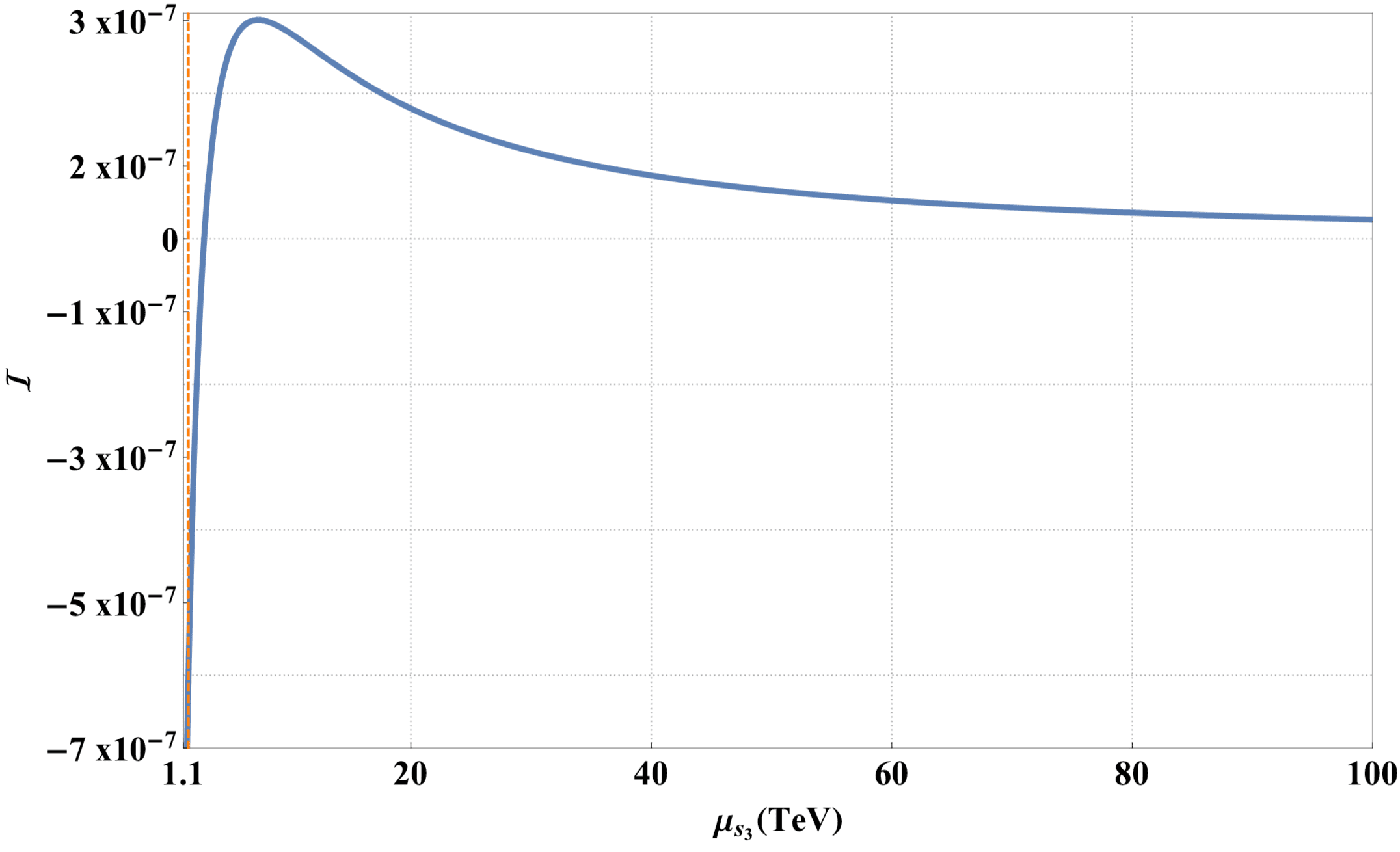
Figure 4: Plot showing the behaviour of the integral, $\mathcal{I}$, (see Equation 18), for leptoquark mass parameter $\mu_{S_{3}}$ ranging from $1.1-100$ TeV. This corresponds to a physical mass range of $m_{r_{1}}=m_{r_{3}}=1.3-118.9$ TeV, while $m_{r_{2}}=m_{r_{4}}$ remains constant for this range. The other exotic mass parameters and the quartic and cubic scalar coupling values have been fixed: $\mu_{S_{1}}=7.5$ TeV, $\mu_{\phi_{3}}=1.5$ TeV, $\lambda_{S_{3}\phi_{3}H}$ = 1 and $m_{S_{1}S_{3}\phi_{3}}=1.5$ TeV. The dashed orange line corresponds to a singularity which exists when $\mu_{S_{3}}=\mu_{S_{1}}$.

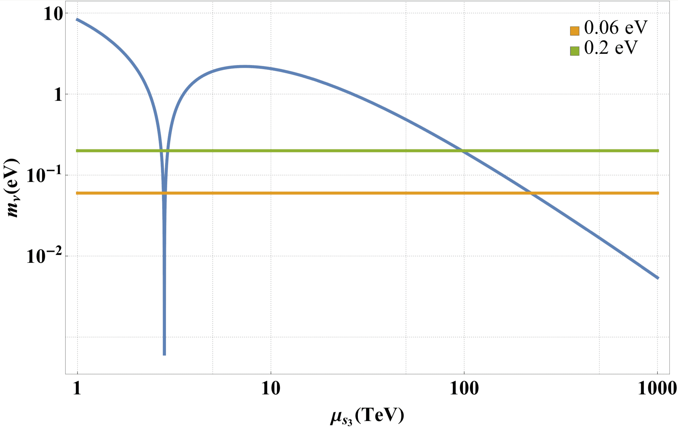
Figure 5: Plot of the sum of neutrino masses, $m_{\nu}$, in eV, for leptoquark mass parameter $\mu_{S_{3}}$ ranging from $1-100$ TeV. The other exotic mass parameters and the quartic and cubic scalar coupling values have been fixed: $\mu_{S_{1}}=7.5$ TeV, $\mu_{\phi_{3}}=1.5$ TeV, $\lambda_{S_{3}\phi_{3}H}$ = 1 and $m_{S_{1}S_{3}\phi_{3}}=1.5$ TeV. All entries in the leptoquark and diquark coupling matrices have been set to $y_{3ij}^{LL}=0.001$ and $z_{1ij}^{LL}=0.01$ respectively. The solid horizontal orange line indicates the experimental lower bound of $0.06$ eV, while the green line shows the approximate cosmological upper limit of $0.2$ eV.

2.4 Casas-Ibarra Parametrisation

After these simplifications the neutrino mass, in the flavour basis, is

$$\begin{split}\boldsymbol{m}_{\nu}=m_{0}(\boldsymbol{y}_{3}^{LL})^{T}\boldsymbol{z}_{1}^{LL}\boldsymbol{y}_{3}^{LL},\end{split}$$ (19)

where we have absorbed all constants into $m_{0}=18m_{S_{1}S_{3}\phi_{3}}\mathcal{I}$ and, for convenience, we define the dimensionless matrix $\kappa\equiv\frac{m_{\nu}}{m_{0}}$. For a given $\kappa$, we thus see that the two coupling matrices, $y_{3}^{LL}$ and $z_{1}^{LL}$, must be related. Their relationship can be obtained using the parametrisation method originally described by Casas and Ibarra Casas:2001sr. Recalling that the diquark couplings $z_{1}^{LL}$ must be symmetric, we can use Takagi’s factorisation method to diagonalise $z_{1}^{LL}=S^{T}D_{z}S$, where $S$ is a unitary matrix, and $D_{z}$ has positive diagonal values. Using $\kappa=U^{*}_{\text{PMNS}}D_{\kappa}U^{\dagger}_{\text{PMNS}}$, where $D_{\kappa}$ is diagonal with positive entries, it follows that

$$\begin{split}D_{\kappa}&=U_{\text{PMNS}}^{T}(y_{3}^{LL})^{T}S^{T}D_{z}Sy_{3}^{LL}U_{\text{PMNS}}\\ &=(\sqrt{D_{z}}Sy_{3}^{LL}U_{\text{PMNS}})^{T}(\sqrt{D_{z}}Sy_{3}^{LL}U_{\text{PMNS}}).\end{split}$$ (20)

Multiplying both sides of the equality by $\sqrt{D_{\kappa}^{-1}}$ on the left and the right, we get

$$\begin{split}\mathds{1}_{3\times 3}=(\sqrt{D_{z}}Sy_{3}^{LL}U_{\text{PMNS}}\sqrt{D_{\kappa}^{-1}})^{T}(\sqrt{D_{z}}Sy_{3}^{LL}U_{\text{PMNS}}\sqrt{D_{\kappa}^{-1}}),\end{split}$$ (21)

where $\mathds{1}_{3\times 3}$ is the identity matrix. This implies that

$$\begin{split}\sqrt{D_{z}}Sy_{3}^{LL}U_{\text{PMNS}}\sqrt{D_{\kappa}^{-1}}=R,\end{split}$$ (22)

where $R$ is an orthogonal matrix (in general with complex entries). Thus, to produce the measured light neutrino masses contained in $D_{\kappa}$, with mixing parameters contained in $U_{\text{PMNS}}$, the most general leptoquark coupling is given by

$$\begin{split}y_{3}^{LL}=S^{\dagger}\sqrt{D_{z}^{-1}}R\sqrt{D_{\kappa}}U_{\text{PMNS}}^{\dagger}.\end{split}$$ (23)

Based on this equation, we see that $y_{3}^{LL}$ depends on the known low-energy parameters contained in $D_{\kappa}$ and $U_{\text{PMNS}}$, as well as the following free parameters: six real parameters from the symmetric diquark coupling, $z_{1}^{LL}$, and three, generally complex, parameters in $R$. Alternatively, since we initially place constraints on $y_{3}^{LL}$, we can rearrange Equation 23 to find $z_{1}^{LL}$ as a function of $y_{3}^{LL}$, such that

$$\begin{split}z_{1}^{LL}=(\sqrt{D_{\kappa}}U_{\text{PMNS}}(y_{3}^{LL})^{-1})^{T}(\sqrt{D_{\kappa}}U_{\text{PMNS}}(y_{3}^{LL})^{-1}).\end{split}$$ (24)

Notice that, due to its symmetric nature, $z_{1}^{LL}$ is independent of the orthogonal matrix $R$. This makes sense since we still have nine free parameters, now all contained in $y_{3}^{LL}$.

2.5 Parameters and notation for analysis

Our model, given the simplifying assumptions, has 14 free parameters: four coming from the mass-dimension 1 couplings $\mu_{S_{1}}$, $\mu_{S_{3}}$, $\mu_{\phi_{3}}$, and $m_{S_{1}S_{3}\phi_{3}}$, and another 10 coming from the dimensionless coupling constants $z_{1}^{LL}$, $y_{3}^{LL}$, and $\lambda_{S_{3}S_{1}H}$, with $z_{1}^{LL}$ and $y_{3}^{LL}$ being related by Equation 24. In Section 3, we discuss several phenomenological constraints on the leptoquark couplings. From here on in, we will simplify our notation such that leptoquark couplings read $(y_{3}^{LL})_{ij}\equiv y_{ij}$, with the index $i$ ($j$) representing the generation of the contributing quark (lepton). We will similarly denote diquark couplings by $(z_{1}^{LL})_{ij}\equiv z_{ij}$.

Given that 14 parameters is too large a space to sample properly, and the results would be difficult to visually present, we are forced to fix the majority of the parameters at benchmark values. We choose to scan over four leptoquark coupling constants, $y_{11}$, $y_{12}$, $y_{21}$ and $y_{22}$, and one mass parameter, $\mu_{S_{3}}$. The benchmark values allocated to $\mu_{S_{1}}$, $\mu_{\phi_{3}}$, $m_{S_{1}S_{3}\phi_{3}}$ and $\lambda_{S_{3}S_{1}H}$ can be found in Table 1. In order to give a representative idea of our model’s robustness as well as investigate a variety of possible conclusions drawn from future particle experiments, Table 1 also includes three benchmark textures for the leptoquark coupling matrix.

$\lambda_{S_{3}S_{1}H}=1$,  $\mu_{S_{1}}=7.5$ TeV,  $\mu_{\phi_{3}}=1.5$ TeV,   $m_{S_{1}S_{3}\phi_{3}}=1.5$ TeV

Texture A	Texture B	Texture C
$y=\begin{pmatrix}y_{11}&y_{12}&\epsilon_{A}\\ y_{21}&y_{22}&5\epsilon_{A}\\ \epsilon_{A}&1&10\epsilon_{A}\end{pmatrix}$	$y=\begin{pmatrix}y_{11}&y_{12}&\epsilon_{B}\\ y_{21}&y_{22}&5\epsilon_{B}\\ \epsilon_{B}&1&10\epsilon_{B}\end{pmatrix}$	$y=\begin{pmatrix}y_{11}&y_{12}&\epsilon_{C}^{2}\\ y_{21}&y_{22}&\epsilon_{C}\\ \epsilon_{C}^{2}&1&1\end{pmatrix}$

Table 1: The parameters $\lambda_{S_{3}S_{1}H}$, $\mu_{S_{1}}$, $\mu_{\phi_{3}}$ and $m_{S_{1}S_{3}\phi_{3}}$ have been fixed to the values indicated. Three different leptoquark coupling matrix textures were used to scan the parameter space, each matrix texture having five of the nine leptoquark couplings fixed, as above, while the other four leptoquark couplings, specifically $y_{11}$, $y_{12}$, $y_{21}$ and $y_{22}$, are scanned over. In texture A, $\epsilon_{A}=10^{-5}$, in texture B, $\epsilon_{B}=10^{-3}$, and in texture C, $\epsilon_{C}=10^{-1}$.

2.6 Model 2 and vanishing neutrino self-energies

Before investigating the phenomenology of Model 1, we will use this section to tie up the loose end of the discarded alternative completion of $O_{47}$. Recall that in Model 2 $S_{3}$ couples as a diquark and $S_{1}$ couples as a leptoquark. When integrated out, these exotic fields give rise to an operator with $\mathrm{SU}(2)$-structure $O_{47}^{k}=\overline{L^{C}}^{i}L^{j}\overline{Q^{C}}^{k}Q^{l}\overline{Q}_{m}Q^{C}_{n}H^{m}H^{n}\epsilon_{ik}\epsilon_{jl}$. Working in two-component Weyl spinor notation, the specific Lorentz structure generated is $(LL)(QQ)(Q^{\dagger}Q^{\dagger})HH$, where parentheses indicate contracted spinors. In Appendix LABEL:App:_vanishing_model we present the calculation of the two-loop contribution to the neutrino mass in this model. Curiously, we find that the neutrino masses vanish due to the symmetry properties of the integral and the antisymmetry of a set of couplings. (This antisymmetry is enforced by Fermi–Dirac statistics.) This suggests that the neutrino mass for this model arises at some higher-loop order. Below we show that the leading-order contribution to the neutrino masses arising from this particle content vanishes. This leading-order argument contains essentially the same ingredients as those required to see the behaviour in the UV theory, and we point readers to the calculation in the appendix for more detail.

Writing all indices ($SU(2)$, $SU(3)$, Lorentz, and flavour) explicitly, Model 1 generates

$$\begin{split}\underset{r}{L}^{\alpha i}\underset{s}{L}^{\beta j}\underset{t}{Q}^{\gamma kA}\underset{u}{Q}^{\delta lB}\underset{v}{Q}^{\dagger}_{\dot{\epsilon}mC}\underset{w}{Q}^{\dagger}_{\dot{\zeta}nD}H^{m}H^{n}\epsilon_{ik}\epsilon_{jl}\epsilon_{\alpha\beta}\epsilon_{\gamma\delta}\epsilon^{\dot{\epsilon}\dot{\zeta}}\epsilon_{ABE}\epsilon^{CDE}\end{split}$$ (25)

at tree level, where Greek letters ($\alpha,\beta,\ldots$) represent spinor indices, Latin letters from the middle of the alphabet ($i,j,\ldots$) represent $SU(2)$ indices, Latin letters from the end of the alphabet ($r,s...$) represent flavour indices and capital letters represent $SU(3)$ indices. The neutrino masses arising from a single insertion of operators of this type will vanish since they depend on integrals with an odd number of loop momenta in the numerator de_Gouv_a_2008. We thus consider neutrino masses arising from insertions of the dimension-13 operator with a derivative acting on each $Q^{\dagger}$. This operator will also be generated by the particle content of the UV-completion of operator $O_{47}^{k}$. However, we now show that this contribution also vanishes.

We first show that the operator must be anti-symmetric under exchange of the $v$ and $w$ flavour indices:

$$\cdots\underset{v}{\partial Q}^{\dagger}_{\epsilon mC}\underset{w}{\partial Q}^{\dagger}_{\zeta nD}H^{m}H^{n}\epsilon^{{\epsilon}{\zeta}}\epsilon^{CDE}\cdots$$

$$= \cdots\underset{v}{\partial Q}^{\dagger}_{{\zeta}nD}\underset{w}{\partial Q}^{\dagger}_{{\epsilon}mC}H^{n}H^{m}\epsilon^{{\zeta}{\epsilon}}\epsilon^{DCE}\cdots {\epsilon}\leftrightarrow{\zeta} m\leftrightarrow n C\leftrightarrow D$$ relabel , and

$$= \cdots\underset{v}{\partial Q}^{\dagger}_{{\zeta}nD}\underset{w}{\partial Q}^{\dagger}_{{\epsilon}mC}H^{n}H^{m}\epsilon^{{\epsilon}{\zeta}}\epsilon^{CDE}\cdots$$ reorder indices

$$= -\cdots\underset{w}{\partial Q}^{\dagger}_{{\epsilon}mC}\underset{v}{\partial Q}^{\dagger}_{{\zeta}nD}H^{n}H^{m}\epsilon^{{\epsilon}{\zeta}}\epsilon^{CDE}\cdots$$ reorder fields

which confirms that the diquark coupling of $S_{3}$ is anti-symmetric in flavour as stated in Dorsner:2016wpm. The neutrino mass generated by this operator is then represented by

$$m_{\nu} =C^{rstu[vw]}(\delta_{tv}\delta_{uw}I_{v}I_{w}+\delta_{tw}\delta_{uv}I_{v}I_{w})+C^{srtu[vw]}(\delta_{tv}\delta_{uw}I_{v}I_{w}+\delta_{tw}\delta_{uv}I_{v}I_{w})$$

$$=(C^{rstu[tu]}+C^{srtu[ut]})I_{u}I_{t}+(C^{srtu[tu]}+C^{srtu[ut]})I_{u}I_{t}$$

$$=0$$

where $C^{rstu[vw]}$ is a Wilson coefficient obtained from the evaluated self-energy diagrams. The square brackets indicate the anti-symmetry under interchange of $v$ and $w$ discussed above.

It should be noted that $O_{47}^{k}$ is missing from the list of $\Delta L=2$ effective operators listed in de_Gouv_a_2008. This may be due to an implicit assumption that the number of SM fermion generations is not more than one. In this case $O_{47}^{k}$ itself vanishes since $Q_{m}Q_{n}H^{m}H^{n}=0$.

One might worry about the validity of this claim in light of the “extended black box” theorem Hirsch_2006, which states that any non-vanishing $\Delta L=2$ effective operator leads to non-vanishing Majorana neutrino mass. This is remedied by the fact that we are only closing off the effective operator in the simplest way to generate neutrino masses. The theorem tells us that there must be non-zero contributions to neutrino mass coming from $O_{47}^{k}$ since the operator itself does not vanish when flavour is considered. We therefore surmise that neutrino masses arise at higher loop order, and are probably too small to meet the lower bound of $\sqrt{|\Delta m^{2}_{32}|}\simeq 0.05$ eV with phenomenologically acceptable exotic particle masses.

There are several other $\Delta L=2$ effective operators which exhibit the same property, including, but not limited to $O_{11b}$, $O_{12a}$ and $O_{48}$. The two-loop contributions coming from completions of all these operators vanish, implying that there must be nonzero higher-loop contributions. Similar remarks about the $0.05$ eV lower bound pertain. This observation could potentially be used to eliminate a sizable number of effective operators from the pool of neutrino-mass-model candidates.

3 Constraints from Rare Processes and Flavour Physics

In this section, we investigate the phenomenology of our Model 1, and place constraints on the values of the coupling constants responsible for generating neutrino mass. This investigation is conducted in three parts. First, the leptoquark couplings $y_{ij}$ are constrained via the model’s BSM contribution to rare processes of charged leptons, including $\mu$ to $e$ conversion in nuclei, the decays $\mu\to e\gamma$ and $\mu\to eee$, and the anomalous magnetic moment of the muon. Second, the leptoquark couplings are constrained via BSM contributions to rare meson decays. Finally, the diquark couplings, $z_{ij}$, are constrained via experimental results from neutral meson anti-meson mixing.

3.1 Rare processes of charged leptons

In the absence of neutrino flavour oscillations, lepton number is conserved in the SM. While lepton flavour has been shown to be violated by neutrino oscillations, it has as-yet not been observed in the charged lepton sector. The lepton flavour violating (LFV) terms in our Lagrangian are thus constrained by charged LFV processes. The most stringent upper bounds on LFV processes in leptoquark models come from $\mu\rightarrow eee$ and $\mu\rightarrow e\gamma$ decays and $\mu-e$ conversion in nuclei.

3.1.1 $\mu\to e$ conversion in nuclei

The strongest bounds on the branching ratio $\mathrm{Br}(\mu\rightarrow e)$ come from $\mu\rightarrow e$ conversion off titanium and gold nuclei. The current constraints, which were set by the SINDRUM Collaboration Dohmen:1993mp; Bertl:2006up, are of order $10^{-12}$ (Table 3.1.1), with future experimental sensitivities predicted to improve by several orders of magnitude. The most promising are the COMET doi:10.1093 and Mu2e/COMET Carey:2008zz experiments, aiming for sensitivities of order $10^{-16}$, and the PRISM/PRIME proposal Yoshitaka2011, boasting a possible sensitivity of $10^{-18}$.

The most general interaction Lagrangian for this process, in the notation of Kitano:2002mt, is

$$\begin{split}\mathcal{L}_{\mu e}^{\rm eff}=&-\frac{4G_{F}}{\sqrt{2}}(m_{\mu}A_{R}\overline{\mu}\sigma^{\mu\nu}P_{L}eF_{\mu\nu}+m_{\mu}A_{L}\overline{\mu}\sigma^{\mu\nu}P_{R}eF_{\mu\nu}+h.c)\\ &-\frac{G_{F}}{\sqrt{2}}\sum_{q=u,d,s}\Big{[}(g_{LS(q)}\overline{e}P_{R}\mu+g_{RS(q)}\overline{e}P_{L}\mu)\overline{q}q\\ &+(g_{LP(q)}\overline{e}P_{R}\mu+g_{RP(q)}\overline{e}P_{L}\mu)\overline{q}\gamma_{5}q\\ &+(g_{LV(q)}\overline{e}\gamma^{\mu}P_{L}\mu+g_{RV(q)}\overline{e}\gamma^{\mu}P_{R}\mu)\overline{q}\gamma_{\mu}q\\ &+(g_{LA(q)}\overline{e}\gamma^{\mu}P_{L}\mu+g_{RA(q)}\overline{e}\gamma^{\mu}P_{R}\mu)\overline{q}\gamma_{\mu}\gamma_{5}q\\ &+\frac{1}{2}(g_{LT(q)}\overline{e}\sigma^{\mu\nu}P_{R}\mu+g_{RT(q)}\overline{e}\sigma^{\mu\nu}P_{L}\mu)\overline{q}\sigma_{\mu\nu}q+\text{h.c.}\Big{]},\end{split}$$ (26)

where $G_{F}$ is the Fermi constant, $m_{\mu}$ is the muon mass, and the $A_{L,R}$ and $g$’s are all dimensionless coupling constants corresponding to the relevant operators.

The branching ratio is defined to be

$$\begin{split}\mathrm{Br}(\mu\rightarrow e)=\frac{\omega_{\mathrm{conv}}}{\omega_{\mathrm{capt}}},\end{split}$$ (27)

where $\omega_{\mathrm{conv}}$ is the $\mu$ to $e$ conversion rate, and $\omega_{\mathrm{capt}}$ is the total muon capture rate. The conversion rate, $\omega_{\mathrm{conv}}$ is calculated from the effective Lagrangian in Equation 26 to be

$$\begin{split}\omega_{\mathrm{conv}}&=2G_{F}^{2}\Big{|}A^{*}_{R}D+\sum_{q}G^{(q,p)}g_{LS(q)}S^{(p)}+\sum_{q}G^{(q,n)}g_{LS(q)}S^{(n)}\\ &+(2g_{LV(u)}+g_{LV(d)})V^{(p)}+(g_{LV(u)}+2g_{LV(d)})V^{(n)}\Big{|}^{2}+(R\leftrightarrow L),\end{split}$$ (28)

where $S$, $D$ and $V$ are overlap integrals, and $n$ and $p$ superscripts refer to processes interacting with a neutron or proton respectively. The coefficients $G^{q,p}$ and $G^{q,n}$, associated with $S^{(p,n)}$, are calculated in Kosmas:2001mv, but do not play a role in our model. This is due to the fact that $\mu\rightarrow e$ conversion does not generate scalar operators in our model, thus $g_{LS(q)}=0$. Similarly, the coefficient associated with tensor operators, namely $A_{R}$, vanishes. Accordingly, we only provide values relevant to our model: the $V$ overlap integral values for titanium and gold can be found in Table 3.1.1, while other values can be found in Kitano:2002mt.

o 0.8X[c] | X[0.5,c] X[0.5,c] |X[c] | X[c]	$V^{(p)}$	$V^{(n)}$	$\mathrm{Br}(\mu\rightarrow e)$	$\omega_{\mathrm{capt}}(10^{6}s^{-1})$
$\phantom{-}{}^{197}_{79}\mathrm{Au}$	0.0610	0.0859	$<7.0\times 10^{-13}$	13.07
$\phantom{-}{}^{48}_{22}\mathrm{Ti}$	0.0462	0.0399	$<4.3\times 10^{-12}$	2.59

Table 2: The relevant overlap integrals in units of $m_{\mu}^{5/2}$, the branching ratio at $90\%$ confidence level and the total capture rates for different nuclei.

(a)

(b)

Figure 6: Tree level processes contributing to $\mu$ to $e$ conversion in nuclei. Note the notation in the left diagram represents two diagrams, one mediated by $r_{1}$ and another by $r_{2}$. The arrows here, as in all other diagrams in this paper. represent the chirality of the field. Arrows pointing towards the vertex represent left-handed fields.

In our model, the dominant contributions to $\mu-e$ conversion in nuclei come from diagrams with the leptoquark $S_{3}$ mediating interactions between the charged leptons and the three lightest quarks, as can be seen in Figure 6. The effective Lagrangian, calculated using Feynman rules for fermion number violating interactions found in Denner:1992vza, is

$$\begin{split}\mathcal{L}^{\text{eff}}_{\mu e}=&-\frac{3}{2}(V_{\text{CKM}}^{*}y)_{12}(V^{*}y)^{\dagger}_{11}\Big{(}\frac{\cos{\theta}}{m_{r_{1}}^{2}}+\frac{\sin{\theta}}{m_{r_{2}}^{2}}\Big{)}[\overline{e}P_{R}u^{c}][\overline{u^{c}}P_{L}\mu]\\ &-\frac{3y_{12}y^{\dagger}_{11}}{m_{S_{3}^{4/3}}^{2}}[\overline{e}P_{R}d^{c}][\overline{d^{c}}P_{L}\mu].\end{split}$$ (29)

After performing a Fierz transformation and separating out the axial vector components (which vanish) from the vector components, we find

$$\begin{split}\mathcal{L}^{\text{eff}}_{\mu e}=&-\frac{3}{8}(V_{\text{CKM}}^{*}y)_{12}(V^{*}y)^{\dagger}_{11}\Big{(}\frac{\cos{\theta}}{m_{r_{1}}^{2}}+\frac{\sin{\theta}}{m_{r_{2}}^{2}}\Big{)}[\overline{e}\gamma^{\mu}P_{L}\mu][\overline{u}\gamma_{\mu}u]\\ &-\frac{3y_{12}y_{11}}{4m_{S_{3}^{4/3}}^{2}}[\overline{e}\gamma^{\mu}P_{L}\mu][\overline{d}\gamma_{\mu}d].\end{split}$$ (30)

Comparison with Equation 26 shows that the nonzero Wilson coefficients are

$$\begin{split}g_{LV(u)}&=\frac{3\sqrt{2}}{8G_{F}}(V_{\text{CKM}}^{*}y)_{12}(V^{*}y)^{\dagger}_{11}\Big{(}\frac{\cos{\theta}}{m_{r_{1}}^{2}}+\frac{\sin{\theta}}{m_{r_{2}}^{2}}\Big{)}.\end{split}$$ (31)

and

$$\begin{split}g_{LV(d)}&=\frac{3\sqrt{2}y_{12}y_{11}}{4G_{F}m_{S_{3}^{4/3}}^{2}}.\end{split}$$ (32)

The matrix element involving strange quarks vanishes as coherent conversion processes dominate and the vector coupling to sea quarks is zero. This leads to

$$\begin{split}\frac{\omega_{\mathrm{conv}}}{\omega_{\mathrm{capt}}}&=\frac{2G_{F}^{2}}{\omega_{\mathrm{capt}}}\Big{|}(2g_{LV(u)}+g_{LV(d)})V^{(p)}+(g_{LV(u)}+2g_{LV(d)})V^{(n)}\Big{|}^{2}.\end{split}$$ (33)

For fixed leptoquark masses, this process places the most stringent constraints on the product $y_{11}y_{12}$ through $\frac{\omega_{\mathrm{conv}}}{\omega_{\mathrm{capt}}}<7.0\times 10^{-13}$ for gold and $<4.3\times 10^{-12}$ for titanium.

3.1.2 $\mu\to e\gamma$

The most stringent constraints on this process are obtained from the non-observation of LFV muonic decays by the MEG experiment TheMEG:2016wtm, with a measured branching ratio of $\mathrm{Br}(\mu\rightarrow e\gamma)=4.2~{}\times~{}10^{-13}\,\text{ at }$ $90\%$ CL. Future prospects are looking to improve on this by an order of magnitude. Specifically, the MEG-II experiment Baldini:2018nnn; Cattaneo:2017psr is predicted to start searching for $\mu\rightarrow e\gamma$ decays this year, with a target sensitivity of $4\times 10^{-14}$. The effective Lagrangian for $\mu\rightarrow e\gamma$ is

$$\begin{split}\mathcal{L}^{\rm eff}_{l\rightarrow l^{\prime}\gamma}=\frac{e}{2}\overline{l^{\prime}}i\sigma^{\mu\nu}F_{\mu\nu}(\sigma_{L}P_{L}+\sigma_{R}P_{R})l,\end{split}$$ (34)

where $l=\mu$ and $l^{\prime}=e$, $\sigma^{\mu\nu}=\frac{i}{2}\left[\gamma^{\mu},\gamma^{\nu}\right]$, $F_{\mu\nu}$ and $\sigma_{L(R)}$ are Wilson coefficients. The partial decay width for $\mu\rightarrow e\gamma$ is

$$\begin{split}\Gamma(\mu\rightarrow e\gamma)=\frac{(m_{\mu}^{2}+m_{e}^{2})^{3}(|\sigma_{L}|^{2}+|\sigma_{R}|^{2})}{16\pi m_{\mu}^{3}}.\end{split}$$ (35)

Our model will have contributions from the leptoquark mass states $r_{1}$ and $r_{2}$ with up-type quarks running in the loop and leptoquark $S_{3}^{4/3}$ with down-type quarks running in the loop, for each of the four diagrams in Figure 3.1.1. In total there are 36 contributing diagrams leading to Wilson coefficients

$$\begin{split}\sigma_{L}=&\phantom{+}\frac{3ie}{16\pi^{2}m^{2}_{S_{3}^{4/3}}}\sum_{q=d_{i}}y_{q1}^{*}y_{q2}m_{e}\left[\frac{4}{3}f_{S}(x_{q})-f_{F}(x_{q})\right]\\ &+\frac{3ie}{16\pi^{2}}\left(\frac{\mathrm{cos^{2}\theta}}{m^{2}_{r_{1}}}+\frac{\mathrm{sin^{2}\theta}}{m^{2}_{r_{2}}}\right)\sum_{q=u_{i}}y_{q1}^{*}y_{q2}m_{e}\left[\frac{1}{3}f_{S}(x_{q})-f_{F}(x_{q})\right],\end{split}$$ (36a)

$$\begin{split}\sigma_{R}=&\phantom{+}\frac{3ei}{16\pi^{2}m^{2}_{S_{3}^{4/3}}}\sum_{q=d_{i}}y_{q1}^{*}y_{q2}m_{\mu}\left[\frac{4}{3}f_{S}(x_{q})-f_{F}(x_{q})\right]\\ &+\frac{3ei}{16\pi^{2}}\left(\frac{\mathrm{cos^{2}\theta}}{m^{2}_{r_{1}}}+\frac{\mathrm{sin^{2}\theta}}{m^{2}_{r_{2}}}\right)\sum_{q=u_{i}}y_{q1}^{*}y_{q2}m_{\mu}\left[\frac{1}{3}f_{S}(x_{q})-f_{F}(x_{q})\right].\end{split}$$ (36b)

Figure 7: There are four types of contributing diagrams to the $\mu\to e\gamma$ process. For our model, each of the four diagrams represents diagrams with either the $S_{3}^{4/3}$ leptoquark and down-type quarks, or $r_{1}$ and $r_{2}$ (electric charge 1/3) and up-type quarks running through the loop.

The Wilson coefficients are summed over the virtual up-type ($u_{i}$) or down-type ($d_{i}$) quark flavours, the factor of 3 comes from the colour contribution and the factors of $4/3$ and $1/3$ come from the electric charges of the relevant leptoquarks. Equations 36a and 36b include contributions from both $r_{1}$ and $r_{2}$, proportional to $\frac{\cos^{2}\theta}{m_{r_{1}}^{2}}$ and $\frac{\sin^{2}\theta}{m_{r_{2}}^{2}}$ respectively. The relevant loop functions are

$$\begin{split}f_{S}(x)&=\frac{x+1}{4(1-x)^{2}}+\frac{x\,\ln x}{2(1-x)^{3}},\\ f_{F}(x)&=\frac{x^{2}-5x-2}{12(x-1)^{3}}+\frac{x\,\ln x}{2(x-1)^{4}},\end{split}$$ (37)

with $x_{q}=m_{q}^{2}/m_{LQ}^{2}$. We thus obtain the following constraint on the leptoquark coupling constants for first and second generation leptons:

$$\begin{split}\mathrm{Br}(\mu\rightarrow e\gamma)=\frac{\Gamma(\mu\rightarrow e\gamma)}{\Gamma_{\mu}^{\mathrm{tot}}}<4.2\times 10^{-13}.\end{split}$$ (38)

where $\Gamma_{\mu}^{\mathrm{tot}}=2.99\times 10^{-19}$ GeV.

3.1.3 Anomalous magnetic moment of the muon

The SM predicts the anomalous magnetic moment of the muon to be $a_{\mu}^{\mathrm{SM}}=1.16591803(70)\times 10^{-3}$ Olive_2014; Davier:2010nc, while the most precise experimental measurement, which comes from the E821 experiment, is $a_{\mu}^{\mathrm{exp}}=1.16592080(63)\times 10^{-3}$. The difference between the SM prediction and the experimental measurement, $\Delta a_{\mu}\equiv a_{\mu}^{\mathrm{exp}}-a_{\mu}^{\mathrm{SM}}=(2.8\pm 0.9)\times 10^{-9}$, suggests the possible presence of BSM contributions. In our model, the leptoquark couplings with the muon provide such a contribution, given by

$$\begin{split}a_{l}=&\phantom{+}\frac{3m_{\mu}}{8\pi^{2}m^{2}_{S_{3}^{4/3}}}\sum_{q=d_{i}}|y_{q2}|^{2}m_{\mu}\left[\frac{4}{3}f_{S}(x_{q})-f_{F}(x_{q})\right]\\ &+\frac{3m_{\mu}}{8\pi^{2}}\left(\frac{\mathrm{cos^{2}\theta}}{m^{2}_{r_{1}}}+\frac{\mathrm{sin^{2}\theta}}{m^{2}_{r_{2}}}\right)\sum_{q=u_{i}}|y_{q2}|^{2}m_{\mu}\left[\frac{1}{3}f_{S}(x_{q})-f_{F}(x_{q})\right].\end{split}$$ (39)

The contribution lies inside the bounds of $\Delta a_{\mu}$, ameliorating the anomaly, without placing a strong constraint on the leptoquark couplings involved. This is consistent with previous results found in literature Cheung_2001; Queiroz_2014; Chakraverty_2001. However, when combined with other leptoquark solutions, the leptoquark $S_{3}$ has been shown to explain the discrepancy between theory and experiment in the anomalous magnetic moment of the muon Dorsner:2019itg.

3.1.4 $\mu\to eee$

To date, the strongest constraint on $\mathrm{Br}(\mu\rightarrow eee)$ remains the $1.0\times 10^{-12}$ achieved by the SINDRUM collaboration in 1988 Bellgardt:1987du. Looking ahead, the Mu3e collaboration Baldini:2018uhj is promising to improve the current constraint by four orders of magnitude. The interaction Lagrangian for this process involves interactions between the $S_{3}$ leptoquark and both the gauge sector and the quark sector. At one-loop level, $\mu\rightarrow eee$ decays receive contributions from three types of Feynman diagrams: $\gamma$- penguins, $Z$-penguins and box diagrams, as depicted in Figure 3.1.1. Thus, the $\mu\rightarrow eee$ probability amplitude consists of three parts

$$\begin{split}\mathcal{A}(\mu\rightarrow eee)=\mathcal{A_{\gamma-\mathrm{penguin}}}+\mathcal{A_{Z-\mathrm{penguin}}}+\mathcal{A_{\mathrm{box}}}.\end{split}$$ (40)

Photon-penguins — The $\mu\rightarrow eee$ photon penguin diagrams closely resemble the $\mu\rightarrow e\gamma$ decay diagrams, however this time the photon is internal, and thus not on-shell. The amplitude for the $\mu\rightarrow eee$ photon penguin diagrams is Hisano:1995cp; Hisano:1998fj; Arganda:2005ji

$$\begin{split}\mathcal{A}_{\gamma-\mathrm{penguin}}&=\overline{\mathbf{u}}_{e}(p_{2})[q^{2}\gamma_{\mu}(A^{L}_{1}P_{L}+A^{R}_{1}P_{R})+im_{\mu}\sigma_{\mu\nu}q^{\nu}(A^{L}_{2}P_{L}+A^{R}_{2}P^{R})]\mathbf{u}_{\mu}(p_{1})\\ &\times\frac{e^{2}}{q^{2}}\overline{\mathbf{u}}_{e}(p_{4})[\gamma_{\mu}]\mathbf{v}_{e}(p_{3})-(p_{2}\leftrightarrow p_{4}),\end{split}$$ (41)

with the Wilson coefficients as follows:

$$\begin{split}A^{L}_{1}&=\frac{3}{16\pi^{2}}\sum_{i=1}^{3}\Bigg{(}\frac{y_{i1}^{*}y_{i2}}{36m_{S_{3}^{4/3}}}F_{1}(x_{i})+\frac{(V_{\text{CKM}}^{*}y)^{*}_{i1}(V_{\text{CKM}}^{*}y)_{i2}\,\mathrm{cos}^{2}\theta}{72m_{r_{1}}^{2}}F_{2}(t_{1i})\\ &+\frac{(V_{\text{CKM}}^{*}y)^{*}_{i1}(V_{\text{CKM}}^{*}y)_{i2}\,\mathrm{sin}^{2}\theta}{72m_{r_{2}}^{2}}F_{2}(t_{2i})\Bigg{)},\\ A^{R}_{1}&=0,\\ A^{L}_{2}&=\sigma_{L},\\ A^{R}_{2}&=\sigma_{R}.\end{split}$$ (42)

(a)

(c)

Figure 8: There are three types of contributing diagrams to the $\mu\rightarrow eee$ process: two types of $\gamma-$ and $Z-$ penguin diagrams, and box Feynman diagrams . For our model, each penguin diagram could have either the $S_{3}^{4/3}$ leptoquark and down-type quarks, or $r_{1}$ and $r_{2}$ (electric charge 1/3) and up-type quarks running through the loop. The situation is similar for the box diagrams, except there will also be contributions where $r_{1}$ and $r_{2}$ are simultaneously present in the loop.

The $\mathbf{u}_{f}$ and $\mathbf{v}_{f}$ are the usual free-particle spinors. The variables in the loop functions are ratios of the squared masses of the quarks and the leptoquarks: $x_{i}=m^{2}_{d_{i}}/m^{2}_{S_{3}^{4/3}}$ and $t_{ji}=m^{2}_{u_{i}}/m^{2}_{r_{j}}$ and the loop functions $F_{1}(x)$ and $F_{2}(x)$ are

$$\begin{split}F_{1}(x)&=\frac{8-27x+36x^{2}-17x^{3}+(4-6x+8x^{3})\,\ln x}{(x-1)^{4}},\\ F_{2}(x)&=\frac{-10+27x-18x^{2}+x^{3}+(-8+12x+x^{3})\,\ln x}{(x-1)^{4}}.\end{split}$$ (43)

These loop functions are not necessarily negligible for the smaller values of $x$ generated by the first and second generations quarks. Thus, since we do not impose a priori restrictions on the leptoquark couplings, $y_{3}$, we cannot neglect the first and second generation contributions here. This also applies to the $Z$-penguin diagrams and the box diagrams where we must also consider all possible combinations of leptoquark mass states and quarks running through the loop. $Z$-penguins — The amplitude of the $Z$-penguin diagrams is

$$\begin{split}\mathcal{A}_{Z-\mathrm{penguin}}=&\frac{1}{m_{Z}^{2}}\overline{\mathbf{u}}_{e}(p_{2})[\gamma_{\mu}(F_{L}P_{L}+F_{R}P_{R})]\mathbf{u}_{\mu}(p_{1})\times\\ \phantom{+}&\overline{\mathbf{u}}_{e}(p_{4})[\gamma_{\mu}(Z_{L}P_{L}+Z_{R}P_{R})]\mathbf{v}_{e}(p_{3})-(p_{2}\leftrightarrow p_{4}),\end{split}$$ (44)

with the Wilson coefficients:

$$\begin{split}F_{L}=&\frac{3}{16\pi^{2}}\sum_{i=1}^{3}\Bigg{(}\frac{y^{*}_{i1}y_{i2}}{2~{}\sin\theta_{W}\,\mathrm{cos}\theta_{W}}F_{3}(x_{i})\\ \phantom{+}&+\frac{(V_{\text{CKM}}^{*}y)^{*}_{i1}(V_{\text{CKM}}^{*}y)_{i2}}{32\,\sin\theta_{W}\,\cos\theta_{W}(t_{1i}-1)^{2}(t_{1i}-t_{2i})(t_{2i}-1)^{2}}F_{4}(t_{1i},t_{2i})\Bigg{)},\\ F_{R}=&0,\\ Z_{L}=&-\frac{e}{\sin\theta_{W}\,\cos\theta_{W}}\left(-\frac{1}{2}+\sin^{2}\theta_{W}\right),\\ Z_{R}=&-e~{}\tan\theta_{W}.\end{split}$$ (45)

Here $\theta_{W}$ is the weak angle, and $x_{i}$ and $t_{ji}$ are as above. We also note that the gauge coupling between the $Z$-boson and leptoquark mass states includes flavour changing contributions. Consequently, the mass states which involve mixing, specifically $r_{1}$ and $r_{2}$, must be treated together when considering the coupling between the Z-boson and the leptoquark $S_{3}$ in the mass basis. The loop functions in 45 are:

$$F_{3}(x)=\frac{x-x^{2}+x\,\ln x}{(x-1)^{2}},$$ (46a)

$$\begin{split}F_{4}(x_{1},x_{2})&=x_{1}^{3}\Bigg{[}4\cos^{2}\theta\bigg{(}\cos 2\theta-2\sin^{2}\theta\,\ln x_{2}-3\bigg{)}\\ &+x_{2}\bigg{(}4\cos 2\theta-\cos 4\theta+8\sin^{2}\theta\,\ln x_{2}-8x_{2}+13\bigg{)}\Bigg{]}\\ &+x_{1}^{2}\Bigg{[}4\cos^{2}\theta\bigg{(}\cos 2\theta\Big{(}2\,\ln x_{1}-2\,\ln x_{2}-3\Big{)}+2\,\ln x_{2}+5\bigg{)}\\ &+x_{2}\bigg{(}3\Big{(}\cos 4\theta-5\Big{)}+\cos 2\theta\Big{(}4-16\cos^{2}\theta\,\ln x_{1}\Big{)}\\ &+4x_{2}\,\cos 2\theta\Big{(}\cos 2\theta\big{(}\ln x_{1}-\ln x_{2}\big{)}+\ln x_{1}+\ln x_{2}-2\Big{)}\\ &-4\sin^{2}\text{$\theta$}\Big{(}\cos 2\theta+5\Big{)}\ln x_{2}+8x_{2}^{2}\bigg{)}\Bigg{]}\\ &+x_{1}\Bigg{[}2\sin^{2}2\theta\bigg{(}\ln x_{1}-\ln x_{2}-2\bigg{)}+x_{2}^{3}\bigg{(}4\cos 2\theta+\cos 4\theta\\ &-8\cos^{2}\theta\,\ln x_{1}-13\bigg{)}+x_{2}^{2}\bigg{(}-\cos 4\theta\Big{(}\ln x_{1}-4\,\ln x_{2}+3\Big{)}\\ &+\cos 2\theta\Big{(}8\ln x_{1}-8\,\ln x_{2}+4\Big{)}+9\,\ln x_{1}+4\,\ln x_{2}+15\bigg{)}\\ &+2x_{2}\bigg{(}\Big{(}\cos 4\theta-3\Big{)}\Big{(}\ln x_{1}-\ln x_{2}\Big{)}-2\cos 2\theta\Big{(}\ln x_{1}+\ln x_{2}+2\Big{)}\bigg{)}\Bigg{]}\\ &+4x_{2}\,\sin^{2}\theta\Bigg{[}2\cos^{2}\theta\bigg{(}\ln x_{1}-\ln x_{2}+2\bigg{)}+x_{2}\bigg{(}x_{2}\Big{(}\cos 2\theta\\ &+2\cos^{2}\theta\,\ln x_{1}+3\Big{)}+\cos 2\theta\Big{(}-2\,\ln x_{1}+2\,\ln x_{2}-3\Big{)}-2\,\ln x_{1}-5\bigg{)}\Bigg{]}.\end{split}$$ (46b)

In the limit of vanishing mixing angle and $x_{1}\rightarrow x_{2}$ we have the following simplification

$$\begin{split}\lim_{\theta\rightarrow 0,x_{1}\rightarrow x_{2}}\frac{F_{4}(x_{1},x_{2})}{(x_{1}-1)^{2}(x_{1}-x_{2})(x_{2}-1)^{2}}=F_{3}(x).\end{split}$$ (47)

Box diagrams — For our model, the non-vanishing amplitude from the contribution of box diagrams to the $\mu\rightarrow eee$ decay is

$$\begin{split}\mathcal{A}_{\mathrm{Box}}=&e^{2}B_{1}^{L}\overline{\mathbf{u}}_{e}(p_{2})[\gamma^{\mu}P_{L}]\mathbf{u}_{\mu}(p_{1})\overline{\mathbf{u}}_{e}(p_{4})[\gamma_{\mu}P_{L}]\mathbf{v}_{e}(p_{3}),\end{split}$$ (48)

with

$$\begin{split}B_{1}^{L}&=\frac{3}{16\pi^{2}e^{2}}\Bigg{\{}\sum_{i,j=1}^{3}2y_{i1}^{*}y_{i2}y_{j1}^{*}y_{j1}D_{00}(m^{2}_{S_{3}^{4/3}},m^{2}_{S_{3}^{4/3}},m^{2}_{d_{i}},m^{2}_{d_{j}})\\ &+(V^{*}_{\text{CKM}}y)_{i1}^{*}(V^{*}_{\text{CKM}}y)_{i2}(V^{*}_{\text{CKM}}y)_{j1}^{*}(V^{*}_{\text{CKM}}y)_{j1}\bigg{[}\cos^{4}\theta\,D_{00}(m^{2}_{r_{1}},m^{2}_{r_{1}},m^{2}_{u_{i}},m^{2}_{u_{j}})\\ &+2\cos^{2}\theta\,\sin^{2}\theta\,D_{00}(m^{2}_{r_{1}},m^{2}_{r_{2}},m^{2}_{u_{i}},m^{2}_{u_{j}})\\ &+\sin^{4}\theta\,D_{00}(m^{2}_{r_{2}},m^{2}_{r_{2}},m^{2}_{u_{i}},m^{2}_{u_{j}})\bigg{]}\Bigg{\}}.\end{split}$$ (49)

The loop function for the box diagrams is defined as

$$\begin{split}m^{2}_{4}D_{00}(m^{2}_{1},m^{2}_{2},m^{2}_{3},m^{2}_{4})=&-\frac{x_{1}^{2}\,\ln x_{1}}{(x_{1}-1)(x_{1}-x_{2})(x_{1}-x_{3})}+\frac{x_{2}^{2}\,\ln x_{2}}{(x_{1}-x_{2})(x_{2}-1)(x_{2}-x_{3})}\\ &+\frac{x_{3}^{2}\,\ln x_{3}}{(x_{1}-x_{3})(x_{3}-1)(x_{3}-x_{2})},\end{split}$$ (50)

where $x_{i}=\frac{m^{2}_{i}}{m^{2}_{4}}$ for $i=1,2,3$. $\mu\rightarrow eee$ Amplitude — Using the form factors defined above, we calculate the $\mu\rightarrow eee$ decay rate to be

$$\begin{split}\Gamma(\mu\rightarrow eee)&=\frac{e^{4}}{512\pi^{3}}m^{5}_{\mu}\Bigg{[}|A_{1}^{L}|^{2}+2(A_{1}^{L}A_{2}^{R*}+\mathrm{h.c.})\\ &+\bigg{(}|A_{2}^{L}|^{2}+|A_{2}^{R}|^{2}\bigg{)}\bigg{(}\frac{16}{3}\,\ln\frac{m_{\mu}}{m_{e}}-\frac{22}{3}\bigg{)}\\ &+\frac{1}{6}|B_{1}^{L}|^{2}+\frac{1}{3}(A_{1}^{L}B_{1}^{L*}+\mathrm{h.c.})-\frac{2}{3}(A_{2}^{R}B_{1}^{L*}+\mathrm{h.c.})\\ &+\frac{1}{3}\bigg{\{}2|F_{LL}|^{2}+|F_{LR}|^{2}+(B_{1}^{L}F_{LL}^{*}+\mathrm{h.c.})\\ &+2(A_{1}^{L}F_{LL}^{*}+\mathrm{h.c.})+(A_{1}^{L}F_{LR}^{*}+\mathrm{h.c.})-4(A_{2}^{R}F_{LL}^{*}+\mathrm{h.c.})\\ &-2(A_{2}^{R}F_{LR}^{*}+\mathrm{h.c.})\bigg{\}}\Bigg{]},\end{split}$$ (51)

with

$$\begin{split}F_{LL}=\frac{F_{L}Z_{L}}{g^{2}\sin^{2}(\theta_{W})m_{Z}^{2}},\qquad F_{LR}=\frac{F_{L}Z_{R}}{g^{2}\sin^{2}(\theta_{W})m_{Z}^{2}}.\end{split}$$ (52)

Thus, we obtain a strong constraint on the leptoquark coupling constants to first and second generation leptons, given by

$$\begin{split}\text{Br}(\mu\rightarrow eee)=\frac{\Gamma(\mu\rightarrow eee)}{\Gamma^{tot}_{\mu}},\end{split}$$ (53)

where $\Gamma^{tot}_{\mu}=2.99\times 10^{-19}$ GeV.

3.2 Rare meson decays

In the SM, rare meson decays in the form of flavour-changing neutral currents (FCNCs) arise at loop level and are thus heavily suppressed, leading them to be highly sensitive to BSM contributions. A plethora of precision experiments have placed stringent bounds on these rare decays. These processes occur at tree-level in our model, thus the couplings involved are severely constrained. Carpentier and Davidson Carpentier:2010ue published a comprehensive list of (order of magnitude) constraints on two-lepton–two-quark ($2l2q$) operators. They work with the effective Lagrangian

$$\begin{split}\mathcal{L}^{\rm eff}_{llqq}\supset\frac{1}{2}\sum^{3}_{i,j,k,n=1}\frac{C_{ijkn}O^{ijkn}_{\alpha}}{m_{\rm NP}^{2}}+\mathrm{h.c.},\end{split}$$ (54)

where $C_{ijkn}/2m_{\rm NP}$ are the Wilson coefficients. The coefficient relevant to our model is that accompanying a dimension six, left-handed chiral vector effective operator

$$\begin{split}O^{ijkn}_{(1)lq}&={(\overline{l_{i}}\gamma^{\mu}P_{L}l_{j})(\overline{q_{k}}\gamma_{\mu}P_{L}q_{n})}\\ &=(\overline{\nu_{i}}\gamma^{\mu}P_{L}\nu_{j}+\overline{e_{i}}\gamma^{\mu}P_{L}e_{j})(\overline{u_{k}}\gamma_{\mu}P_{L}u_{n}+\overline{d_{k}}\gamma_{\mu}P_{L}d_{n}).\end{split}$$ (55)

The bounds are set on dimensionless coefficients, $\epsilon^{ijkn}_{(n)lq}$, related to the respective Wilson coefficients by

$$\begin{split}\frac{C^{ijkn}_{(1)lq}}{m^{2}_{\rm NP}}=-\frac{4G_{F}}{\sqrt{2}}\epsilon^{ijkn}_{(1)lq}.\end{split}$$ (56)

Bounds are placed on $\epsilon^{ijkn}$ by analysing the contribution of a relevant effective operator to the branching ratios of rare meson decays, one effective operator at a time. In doing so, there is a risk of overlooking possible destructive interference effects. Therefore, the constraints in this section are only order of magnitude estimates. The analysis discussed in this section allows us to place constraints on all nine leptoquark couplings, $y_{ij}$, through simply calculating the contribution of leptonic rare meson decays and semi-leptonic neutral current decays to $2l2q$ effective operators. The results are summarised in Table LABEL:table:_constraints_on_2l2q_processes.

Figure 9: Dominant contributions to $K^{0}_{L}\rightarrow\overline{e}\mu$ ($K^{0}_{L}\rightarrow\overline{\mu}\mu$).

3.2.2 Semi-leptonic meson decays

The semi-leptonic meson decays, the most tightly constrained being $K^{+}\rightarrow\pi^{+}\overline{\nu}\nu$ and $B^{+}\rightarrow K^{+}\overline{\nu}\nu$, place bounds on third generation leptoquark couplings, as well as additional bounds on the couplings already discussed. The process $K^{+}\rightarrow\pi^{+}\overline{\nu}\nu$, depicted in Figure 3.1.1, induces the following Wilson coefficient, associated with the operator $O^{ij12}_{(1)lq}=(\overline{\nu_{i}}\gamma^{\mu}P_{L}\nu_{j})(\overline{d}\gamma^{\mu}P_{L}s)$:

$$\begin{split}\frac{C_{(1)lq}^{ij12}}{m_{LQ}^{2}}=\sum_{i,j=1}^{3}\frac{y_{1i}y_{2j}}{2}\left(\frac{\cos{\theta}}{m_{r_{1}}^{2}}+\frac{\sin{\theta}}{m_{r_{2}}^{2}}\right),\end{split}$$ (58)

where we sum over the neutrino flavour. The bounds on $\epsilon^{ijkn}$, found in Table LABEL:table:_constraints_on_2l2q_processes, are calculated one flavour at a time, with all other contributions set to zero. After this analysis, the only unconstrained leptoquark parameters are those involving third generation quarks. The leptoquark couplings to third generation quarks can be constrained via the process $B^{+}\rightarrow K^{+}\overline{\nu}\nu$, which induces the effective operator $O^{ij23}_{(1)lq}=(\overline{\nu_{i}}\gamma^{\mu}P_{L}\nu_{j})(\overline{s}\gamma^{\mu}P_{L}b)$. The Feynman diagram associated with this operator is pictured in Figure 3.1.1, and the Wilson coefficients $\frac{C^{ij23}}{m_{LQ}^{2}}$, are identical to Equation 58 apart from the quark indices. The constraints applied to each set of parameters are summarised in Table LABEL:table:_constraints_on_parameters_from_2q2l_operators. Note that we do not include constraints from the anomalous decay $B_{s}\rightarrow\overline{\mu}\mu$, which will be discussed in Section 3.4.

(a)

(b)

Figure 10: Dominant contributions to (a) $K^{+}\rightarrow\pi^{+}\overline{\nu}\nu$ and (b) $B^{+}\rightarrow K^{+}\overline{\nu}\nu$.

The SM Wilson coefficient for meson mixing is

$$\begin{split}C_{1,SM}^{ij}=-\frac{G_{F}^{2}m_{W}}{12\pi^{2}}V_{ti}^{2}V_{tj}^{*2}S_{0}\left(\frac{m_{t}^{2}}{m_{W}^{2}}\right),\end{split}$$ (61)

where $m_{t}$ is the mass of the top quark, $m_{W}$ is the mass of the $W$ boson and $S_{0}(x)$ is the Inami-Lim function Inami:1980fz,

$$\begin{split}S_{0}(x)=x\left(\frac{1}{4}+\frac{9}{4}\frac{1}{1-x}\right)-\frac{3}{2}\left(\frac{x}{1-x}\right)^{3}.\end{split}$$ (62)

Figure 11: Dominant contributions to $K-\overline{K}$ mixing.

As can be seen in Figure 3.1.1, which depicts the NP Feynman diagrams for kaon mixing, our model contributes to meson mixing through box diagrams with both diquark and leptoquark propagators. When considering the contributions from the diquark, $S_{1}$, we only include contributions which include the top quark as a propagator, just as in the SM calculation. This is because the CKM matrix elements involving the top quark dominate over the others. Leptoquark contributions occur through box diagrams with either neutrinos and $r_{1,2}$ or charged leptons and $S_{3}^{4/3}$. Summing over all contributions, we have the following BSM Wilson coefficient for meson mixing

$$\begin{split}C^{ij}_{1,{\rm NP}}=&-\frac{(zV_{\text{CKM}}^{\dagger})^{2}_{3i}(V_{\text{CKM}}^{*}z)^{2}_{3j}}{96\pi^{2}m_{S_{1}}^{2}}-\frac{1}{96\pi^{2}}\left(\sum_{k}\frac{y_{ik}y_{jk}}{m_{S_{3}^{4/3}}\pi}\right)^{2}\\ &-\frac{1}{384\pi^{2}}\left(\sum_{k}y_{ik}y_{jk}\right)^{2}\left[\left(\frac{\cos{\theta}}{m_{r_{1}}}\right)^{2}+\left(\frac{\sin{\theta}}{m_{r_{2}}}\right)^{2}+\frac{2\sin{\theta}\,\cos{\theta}}{m_{r_{1}}^{2}-m_{r_{2}}^{2}}\mathrm{ln}\frac{m_{r_{1}}^{2}}{m_{r_{2}}^{2}}\right].\end{split}$$ (63)

The effective operators and Wilson coefficients depend on the renormalisation scheme and scale. However, since we are only interested in an order of magnitude estimate, we neglect the running from the scale of new physics to the top quark mass and take the ratio of the new physics contribution to the SM contribution. This ratio is independent of QCD running and is simply a ratio of the respective Wilson coefficients,

$$\begin{split}\frac{\bra{M}\mathcal{H}^{\rm NP}_{\rm eff}\ket{\overline{M}}}{\bra{M}\mathcal{H}^{\rm SM}_{\rm eff}\ket{\overline{M}}}=\frac{C_{1,{\rm NP}}^{ij}}{C_{1,{\rm SM}}^{ij}}.\end{split}$$ (64)

The UTfit collaboration has published model-independent constraints on $\Delta F=2$ operators Bona:2007vi, with the results from the latest fit published in UTFitweb:

$$\begin{split}C_{B_{q}}e^{2i\phi_{B_{q}}}&=\frac{\bra{B_{q}}\mathcal{H}_{\rm eff}^{\rm full}\ket{\overline{B}_{q}}}{\bra{B_{q}}\mathcal{H}_{\rm eff}^{\rm SM}\ket{\overline{B}_{q}}}=1+\frac{\bra{B_{q}}\mathcal{H}_{\rm eff}^{\rm NP}\ket{\overline{B}_{q}}}{\bra{B_{q}}\mathcal{H}_{\rm eff}^{\rm SM}\ket{\overline{B}_{q}}}\end{split}$$ (65a)

$$\begin{split}C_{\Delta m_{K}}&=\frac{\mathrm{Re}[\bra{K}\mathcal{H}_{\rm eff}^{\rm full}\ket{\overline{K}}]}{\mathrm{Re}[\bra{K}\mathcal{H}_{\rm eff}^{\rm SM}\ket{\overline{K}}]}=1+\frac{\mathrm{Re}[\bra{K}\mathcal{H}_{\rm eff}^{\rm NP}\ket{\overline{K}}]}{\mathrm{Re}[\bra{K}\mathcal{H}_{\rm eff}^{\rm SM}\ket{\overline{K}}]}\end{split}$$ (65b)

$$\begin{split}C_{\Delta\epsilon_{K}}&=\frac{\mathrm{Im}[\bra{K}\mathcal{H}_{\rm eff}^{\rm full}\ket{\overline{K}}]}{\mathrm{Im}[\bra{K}\mathcal{H}_{\rm eff}^{\rm SM}\ket{\overline{K}}]}=1+\frac{\mathrm{Im}[\bra{K}\mathcal{H}_{\rm eff}^{\rm NP}\ket{\overline{K}}]}{\mathrm{Im}[\bra{K}\mathcal{H}_{\rm eff}^{\rm SM}\ket{\overline{K}}]}.\end{split}$$ (65c)

The current best fit values for these parameters are given by UTFitweb

$$\begin{split}\begin{tabular}[]{lll}$C_{B_{d}}=1.03\pm 0.11$,&\phantom{blankspaces}&$\phi_{B_{d}}=-1.8^{\circ}\pm 1.7^{\circ}$,\\ $C_{B_{s}}=1.070\pm 0.088$,&\phantom{blankspaces}&$\phi_{B_{s}}=0.054^{\circ}\pm 0.951^{\circ}$,\\ $C_{\Delta m_{K}}=0.978\pm 0.331$,&\phantom{blankspaces}&$C_{\epsilon_{K}}=1.04\pm 0.11$.\end{tabular}\end{split}$$ (66)

As can be seen in Equation 66, $\phi_{B_{d}}$ and $\phi_{B_{s}}$ are not measured precisely, thus in placing constraints on B–meson mixing we simply require that the magnitude of the right-handed side of Equation 65a be within the one standard deviation range of $C_{B_{d}}$ and $C_{B_{s}}$, as per the values quoted in Equation 66. Specifically

$$\begin{split}0.92<\left|1+\frac{C_{1,{\rm NP}}^{13}}{C_{1,{\rm SM}}^{13}}\right|<1.14\end{split}$$ (67)

for $B_{d}$ mixing, and

$$\begin{split}0.982<\left|1+\frac{C_{1,{\rm NP}}^{23}}{C_{1,{\rm SM}}^{23}}\right|<1.158\end{split}$$ (68)

for $B_{s}$ mixing. Concerning the bounds placed on couplings involved in kaon mixing, only the imaginary part of the ratio of NP to SM Wilson coefficients, seen in Equation 65c, was constrained:

$$\begin{split}\frac{C_{1,{\rm NP}}^{ij}}{C_{1,{\rm SM}}^{ij}}<0.15.\end{split}$$ (69)

3.4 Solving the $R_{K^{(*)}}$ anomaly

While not the focus of this paper, another key feature of our model is its ability to explain the $R_{K{(*)}}$ flavour anomalies due to the presence of the $S_{3}$ scalar leptoquark. The $R_{K^{(*)}}$ flavour anomalies are a set of deviations from SM predictions in the decays of B-mesons. The anomalous quantities are the ratios of branching fractions

$$\begin{split}R_{K^{(*)}}=\frac{\text{Br}(\overline{B}\rightarrow\overline{K}^{(*)}\mu\mu)}{\text{Br}(\overline{B}\rightarrow\overline{K}^{(*)}ee)}.\end{split}$$ (70)

The SM prediction of $R_{K^{(*)}}=1.0003\pm 0.0001$ Bobeth:2007dw is close to unity due to lepton flavour universality, with the only difference in the measured branching fractions coming from their dependence on the masses of the final state leptons. Most recently, the LHCb collaboration has updated the measurement of $R_{K}$ by combining Run-1 data with 2 ${\rm fb}^{-1}$ of Run-2 data Aaij:2019wad. They found

$$\begin{split}R_{K}=0.846^{+0.060~{}+0.016}_{-0.054~{}-0.014},~{}~{}~{}~{}~{}~{}~{}q^{2}=[1.1,6]\ \mathrm{GeV}^{2},\end{split}$$ (71)

where $q^{2}$ is the dilepton invariant mass squared, the first uncertainty is statistical and the second is systematic. This result continues to be in tension with theory at $2.5\sigma.$ The $R_{K^{*}}$ results have also been updated, with preliminary measurements by Belle Abdesselam:2019wac of

$$\begin{split}R_{K^{*}}&=\begin{dcases}0.90^{+0.27}_{-0.21}\pm 0.10~{}~{}q^{2}=[0.1,8]\ \mathrm{GeV}^{2}\\ 1.18^{+0.52}_{-0.32}\pm 0.10~{}~{}q^{2}=[15,19]\ \mathrm{GeV}^{2},\end{dcases}\end{split}$$ (72)

in agreement with the existing measurements by LHCb Aaij:2017vbb of

$$\begin{split}R_{K^{*}}&=\begin{dcases}0.660^{+0.110}_{-0.070}\pm 0.024~{}~{}q^{2}=[0.045,1.1]~{}\mathrm{GeV}^{2}\\ 0.685^{+0.113}_{-0.069}\pm 0.047~{}~{}q^{2}=[1.1,6]~{}\mathrm{GeV}^{2}.\end{dcases}\end{split}$$ (73)

Interestingly, the large uncertainties in the Belle measurement allow it to be in agreement with both the SM and the LHCb measurement, which deviates from the SM prediction by $\sim 2.5\sigma$. Our model contributes to $R_{K^{(*)}}$ via semi-leptonic B-meson decays mediated by $S_{3}$. The $b\rightarrow sll$ transition can be described by the effective Hamiltonian

$$\begin{split}\mathcal{H}_{\rm eff}=-\frac{4G_{F}}{\sqrt{2}}(V_{\text{CKM}})_{33}(V_{\text{CKM}})_{32}^{*}\frac{\alpha_{e}}{4\pi}\sum_{i}C_{i}(\mu)O_{i}(\mu),\end{split}$$ (74)

where $\alpha_{e}$ is the fine structure constant. The relevant effective operator for our model, presented here in the chiral basis, is

$$\begin{split}O^{\mu\mu}_{LL}=(\overline{\mu}\gamma_{\nu}P_{L}\mu)(\overline{s}\gamma_{\nu}P_{L}b).\end{split}$$ (75)

Reference Aebischer:2019mlg argues that contributions to the effective operator $O_{LL}^{\mu\mu}$ with Wilson coefficient

$$\begin{split}C^{\mu\mu}_{LL}=\frac{\pi}{\alpha_{e}}\frac{y_{22}y_{32}}{(V_{\text{CKM}})_{33}(V_{\text{CKM}})^{*}_{32}}\frac{\sqrt{2}}{2m_{S_{3}^{4/3}}^{2}G_{F}}\approx-0.53\pm 0.08(0.16),\end{split}$$ (76)

ameliorates the $R_{K^{(*)}}$ anomalies, with the uncertainties giving the $1(2)\sigma$ bounds. In our model, this corresponds to a central value of

$$\begin{split}y_{22}y_{32}\approx\Big{(}\frac{m_{S_{3}^{4/3}}}{35~{}\mathrm{TeV}}\Big{)}^{2}.\end{split}$$ (77)

4 Results

We will now present the results of our random parameter scans, and discuss the predictions and limitations of the model. The discussion is broken up into three sections, each discussing one of the three leptoquark coupling matrix textures introduced in Table 1. The strongest constraint on the model comes from $\mu\rightarrow e$ conversion in gold nuclei, which is mediated by leptoquark $S_{3}$ at tree level. Consequently, we will also explore the potential consequences for the model if future $\mu\rightarrow e$ experiments fail to measure a signal at the promised prospective sensitivities. The scans were performed over leptoquark couplings $y_{11},$ $y_{12}$, $y_{21}$ and $y_{22}$, and the leptoquark mass parameter $\mu_{S_{3}}$, with all other couplings fixed. In 2018 the CMS experiment at the LHC set an exclusion on diquark masses below $7.2$ TeV at $95\%$ confidence interval Sirunyan:2018xlo. While the exclusion was calculated for a particular diquark which features in superstring inspired $E_{6}$ models HEWETT1989193, similar bounds are expected to apply to other diquarks. The CMS experiment has also set limits on leptoquarks masses, with masses below $1.1$ TeV being excluded at $95\%$ confidence interval for third generation leptoquarks decaying to $b\nu$ Sirunyan:2018kzh. We are not aware of current limits on exotic scalars that only couple to other scalars and gauge bosons, such as $\phi_{3}$. With these considerations in mind, we stick to conservative lower bounds that have the potential to be directly probed at the LHC and indirectly probed at precision- or luminosity-frontier experiments. We fix the diquark mass parameter in our model to a benchmark value of $\mu_{S_{1}}=7.5$ TeV, the mass parameter for the scalar $\phi_{3}$ to $\mu_{\phi_{3}}=1.5$ TeV, and scan over the leptoquark mass parameter such that $1.1\leq\mu_{S_{3}}\leq 10~{}\text{TeV}$. The limits on leptoquark masses are set assuming sufficiently large leptoquark couplings of $y\geq 10^{-7}$ to guarantee prompt decay of leptoquarks in the detector. We also found that due to the relationship between $y_{3}^{LL}$ and $z_{1}^{LL}$ displayed in Equation 24, leptoquark couplings below $10^{-5}$ had a high likelihood of requiring large, non-perturbative diquark couplings in order to guarantee the desired neutrino masses. Thus, the free leptoquark couplings: $y_{11},$ $y_{12}$, $y_{21}$ and $y_{22}$ are allowed to vary between $10^{-5}$ and $1$. The other five leptoquark couplings are set to benchmark values. We investigate three leptoquark matrix textures, as indicated in Table 1 and detailed below.

4.1 Texture A

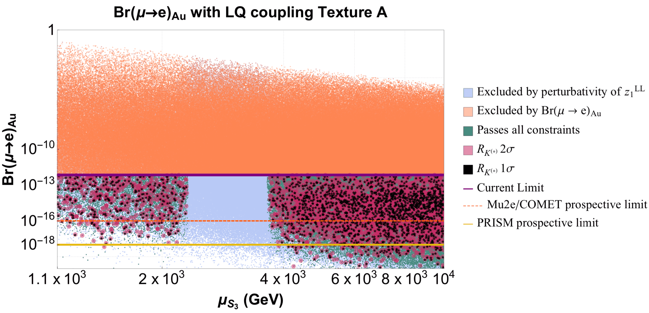
Figure 12: Indicative plot of the allowed parameter space scans showing $\mu_{S_{3}}$ vs. $\text{Br}(\mu~{}\rightarrow~{}e)_{\text{Au}}$, for leptoquark coupling matrix Texture A. The purple line indicates the current $\text{Br}(\mu~{}\rightarrow~{}e)_{\text{Au}}$ cut-off of $7.0\times 10^{-13}$, and the dotted orange (yellow) line indicates the prospective cut-off from the Mu2e/COMET (PRISM) experiment which is of order $10^{-16}$ ($10^{-18}$). The orange region of the parameter space is constrained by $\text{Br}(\mu~{}\rightarrow~{}e)_{\text{Au}}$, the teal region is allowed; specifically it passes all constraints discussed in Section 3 as well as perturbativity constraints on the diquark coupling constants $z^{LL}_{1ij}$. The light blue region is excluded by the perturbativity constraints on diquark couplings. The black (pink) region solves the $R_{K^{(*)}}$ anomalies to $1(2)\sigma$.

The leptoquark matrix texture investigated first is Texture A

$$\begin{split}y=\begin{pmatrix}y_{11}&y_{12}&\epsilon_{A}\\ y_{21}&y_{22}&5\epsilon_{A}\\ \epsilon_{A}&1&10\epsilon_{A}\end{pmatrix},\end{split}$$ (78)

with $\epsilon_{A}=10^{-5}$. If leptoquark couplings to third generation quarks and leptons are very weak, as they are for Texture A, ample parameter space is available when accounting for current constraints, including regions which allow the model to explain the $R_{K^{(*)}}$ flavour anomalies, as summarised in Figures 12, 13 and 14. In fact, with leptoquark couplings of the order of $\sim 10^{-5}$, this neutrino mass model is able to explain $R_{K^{(*)}}$ at a $1\sigma$ level even if NP is not discovered by future experiments, such as Mu2e/COMET and PRISM. This is evident in Figure 12, where viable parameter space is plotted in teal, points that solve the $R_{K^{(*)}}$ anomalies to $1(2)\sigma$ are black (pink) and the dotted orange (yellow) lines represent prospective constraints for $\text{Br}(\mu\rightarrow e)_{\text{Au}}$ from the Mu2e/COMET (PRISM) experiments.

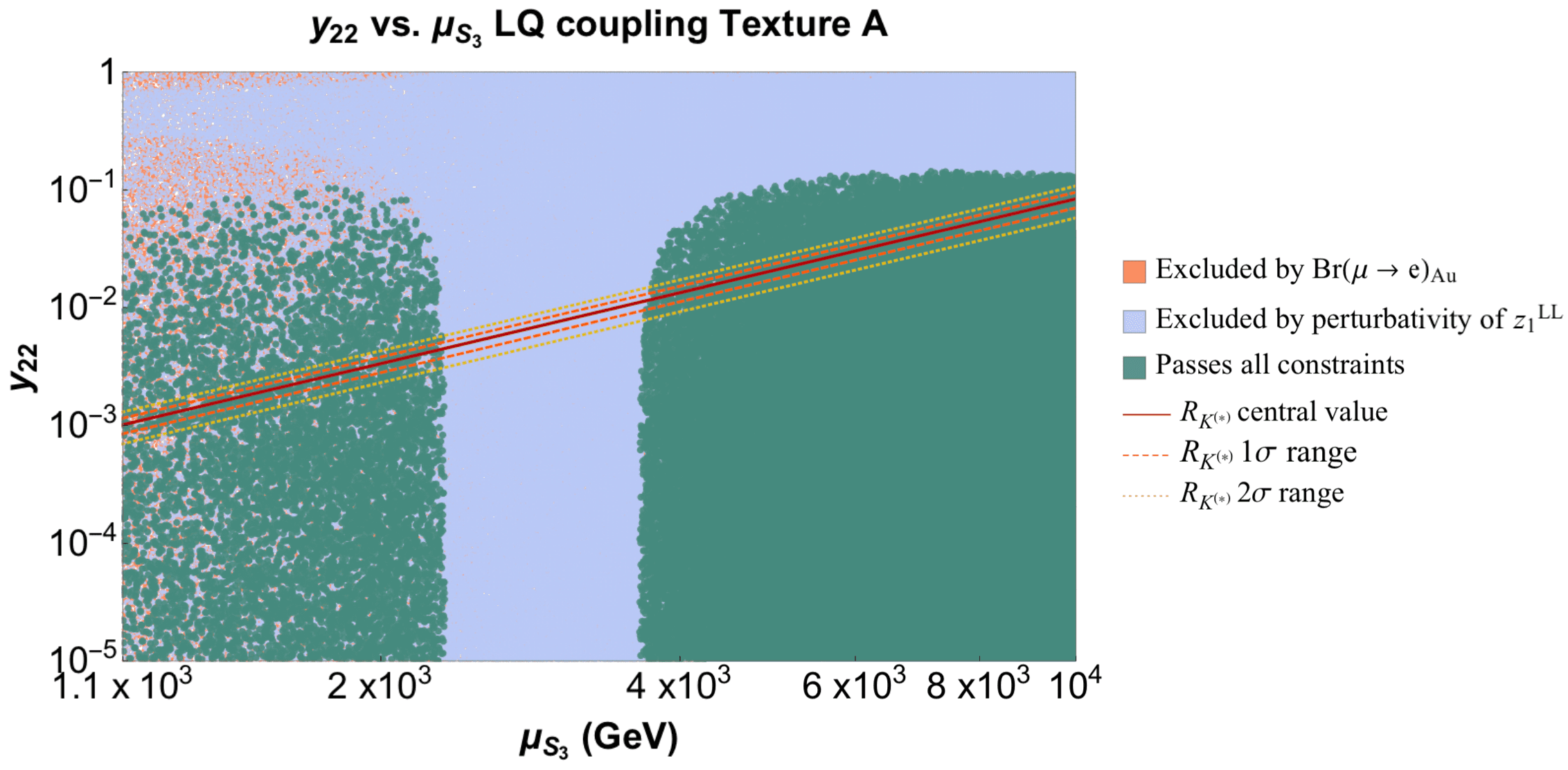
Figure 13: Indicative plot of the allowed parameter space in the $y_{22}$ vs. $\mu_{S_{3}}$ plane, for leptoquark coupling matrix Texture A. The red line indicates the central value needed to explain the $R_{K^{(*)}}$ anomalies with the dotted orange (yellow) lines indicating the $1(2)~{}\sigma$ bounds. The orange region of the parameter space is constrained by $\text{Br}(\mu\rightarrow e)_{\text{Au}}$, the teal region is allowed; specifically it passes all constraints discussed in Section 3 as well as perturbativity constraints on the diquark coupling constants $z^{LL}_{1ij}$. The light blue region is excluded by perturbativity constraints on diquark couplings.

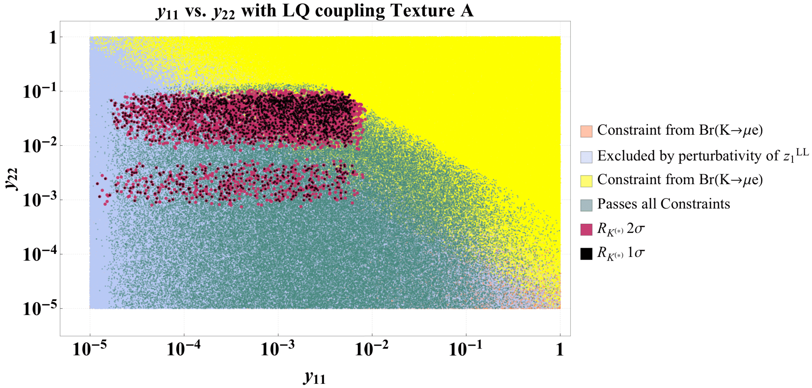
Figure 14: Indicative plot of the allowed parameter space in the $y_{22}$ vs. $y_{11}$ plane, for leptoquark coupling matrix Texture A. The yellow section is ruled out by $\text{Br}(K\rightarrow\mu e)$, the orange section is ruled out by $\text{Br}(\mu\rightarrow e)_{\text{Au}}$, while the teal region is allowed parameter space; specifically it passes all constraints discussed in Section 3 as well as perturbativity constraints on the diquark coupling constants $z^{LL}_{1ij}$. The light blue region is excluded by perturbativity constraints on diquark couplings.

Figures 12 and 13 both contain a curious feature: a region of parameter space (in the form of a band in $\mu_{S_{3}}$) which is excluded due to perturbativity constraints placed on the diquark coupling constants. This feature can be understood as follows. Small leptoquark couplings lead to a higher probability of non-perturbative diquark couplings. This is a consequence of Equation 24, which parametrises the diquark couplings in terms of the leptoquark couplings to ensure the desired neutrino masses are computed. The value of $z_{1}^{LL}$ is also inversely proportional to the value of the integral. The curious feature of the band of excluded parameter space in the $\mu_{S_{3}}\sim 2-4$ TeV, displayed in Figures 12 and 13, corresponds to the sign change in the integral. This can be verified in Figure 4. Simply put, there exits a region of $\mu_{S_{3}}$ for which the value of the leptoquark coupling and the integral are sufficiently small, making the diquark couplings $z_{1ij}^{LL}$ too large to be perturbative. The $R_{K^{(*)}}$ anomalies can be solved for a sub-region of the allowed parameter space, for $y_{11}\lesssim 10^{-2}$ and $10^{-3}\lesssim y_{22}\lesssim 10^{-1}$. There is a band around $y_{22}\simeq 10^{-2}$ for which the model cannot explain the $R_{K^{(*)}}$ anomalies, which corresponds to the non-perturbative band in Figure 13. Figure 14 also shows that while $\mu\rightarrow e$ conversion is found to be the most constraining process for this model in general as it appears at tree level, there are other important signals. Since the neutrino mass of this model does not depend on quark masses, there is no reason to set couplings to first generation quarks to zero, meaning our model is also sensitive to probes involving first generation quarks, such as $K^{0}_{L}\rightarrow\bar{e}\mu$ and $K^{+}\rightarrow\pi^{+}\bar{\nu}\nu$. The process $K^{0}_{L}\rightarrow\bar{e}\mu$ is the most constraining for our model, with Figure 14 showing that the leptoquark couplings $y_{11}$ and $y_{22}$ cannot be simultaneously close to unity. There exists a trade off due largely to constraints coming from $\text{Br}(K\rightarrow\mu e)$. It should be noted that $\mu\rightarrow e$ conversion, shown in orange in Figures 14 and 13, is also strongly constraining in the regions excluded by perturbativity and $\text{Br}(\mu\rightarrow e)_{\text{Au}}$ constraints.

4.2 Texture B

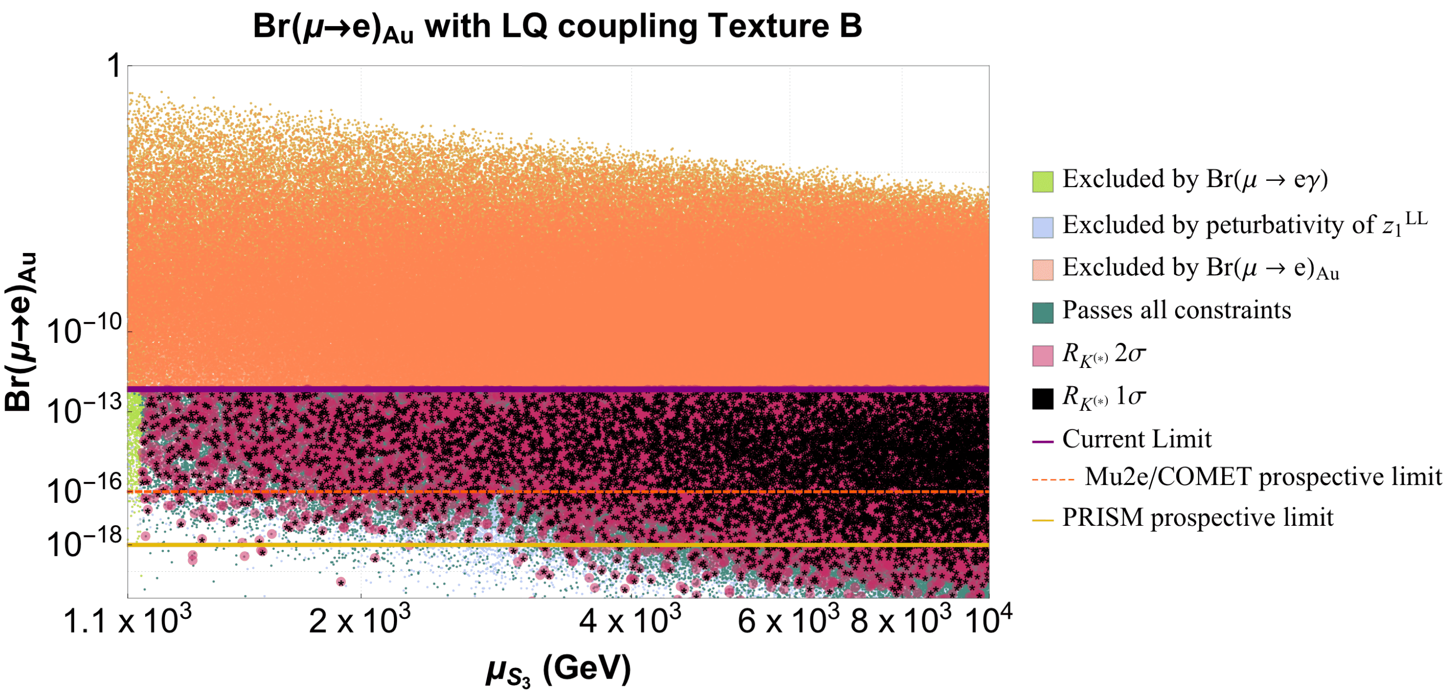
Figure 15: Indicative plot of the allowed parameter space scans showing $\mu_{S_{3}}$ vs. $\text{Br}(\mu~{}\rightarrow~{}e)_{\text{Au}}$, for leptoquark coupling matrix Texture B. The purple line indicates the current $\text{Br}(\mu~{}\rightarrow~{}e)_{\text{Au}}$ cut-off, the dotted orange (yellow) line indicates the prospective cut-off from the Mu2e/COMET (PRISM) experiment. The light green region shows parameter space that is excluded by $\text{Br}(\mu~{}\rightarrow~{}e\gamma)$. The orange region of the parameter space is constrained by $\text{Br}(\mu~{}\rightarrow~{}e)_{\text{Au}}$, the teal region is allowed; specifically it passes all constraints discussed in Section 3 as well as perturbativity constraints on the diquark coupling constants $z^{LL}_{1ij}$. The black (pink) region solves the $R_{K^{(*)}}$ anomalies to $1(2)\sigma$.

The leptoquark matrix texture considered next is Texture B

$$\begin{split}y=\begin{pmatrix}y_{11}&y_{12}&\epsilon_{B}\\ y_{21}&y_{22}&5\epsilon_{B}\\ \epsilon_{B}&1&10\epsilon_{B}\end{pmatrix},\end{split}$$ (79)

where $\epsilon_{B}=10^{-3}$. For this leptoquark matrix coupling texture, constraints due to the perturbativity of the diquark couplings are no longer a major concern. Texture B gives similar results to Texture A in that it is strongly constrained by $\text{Br}(\mu\rightarrow e)_{\text{Au}}$ and $\text{Br}(K\rightarrow\mu e)$, yet still able to solve the $R_{K^{(*)}}$ anomalies. In fact, with leptoquark couplings to third generation quarks of order $10^{-3}$, there exists parameter space which is able to solve the $R_{K^{(*)}}$ anomalies to $1\sigma(2\sigma)$ even if NP is not discovered by future experiments such as Mu2e/COMET and PRISM, as can be seen in Figure 15 in black (pink). Figure 15 also shows, in light green, that we now have a constraint from $\text{Br}(\mu\rightarrow e\gamma)$ on the leptoquark mass parameter $\mu_{S_{3}}$. As for Texture A, leptoquark couplings of $y_{11}\lesssim 10^{-2}$ and $10^{-3}\lesssim y_{22}\lesssim 10^{-1}$ can currently solve the $R_{K^{(*)}}$ anomalies, as depicted in Figure 17. In can also be seen that $y_{22}$ must be less than unity, or the model is not viable at all due to constraints from $\mu\rightarrow e$ conversion. Constraints from $\text{Br}(K\rightarrow\mu e)$ enforces a trade off between large $y_{11}$ and $y_{22}$ couplings for Texture B. additionally, Figure 16 shows that $y_{22}\lesssim 10^{-1}$ is necessary for $\mu_{S_{3}}\simeq 1.2$ TeV.

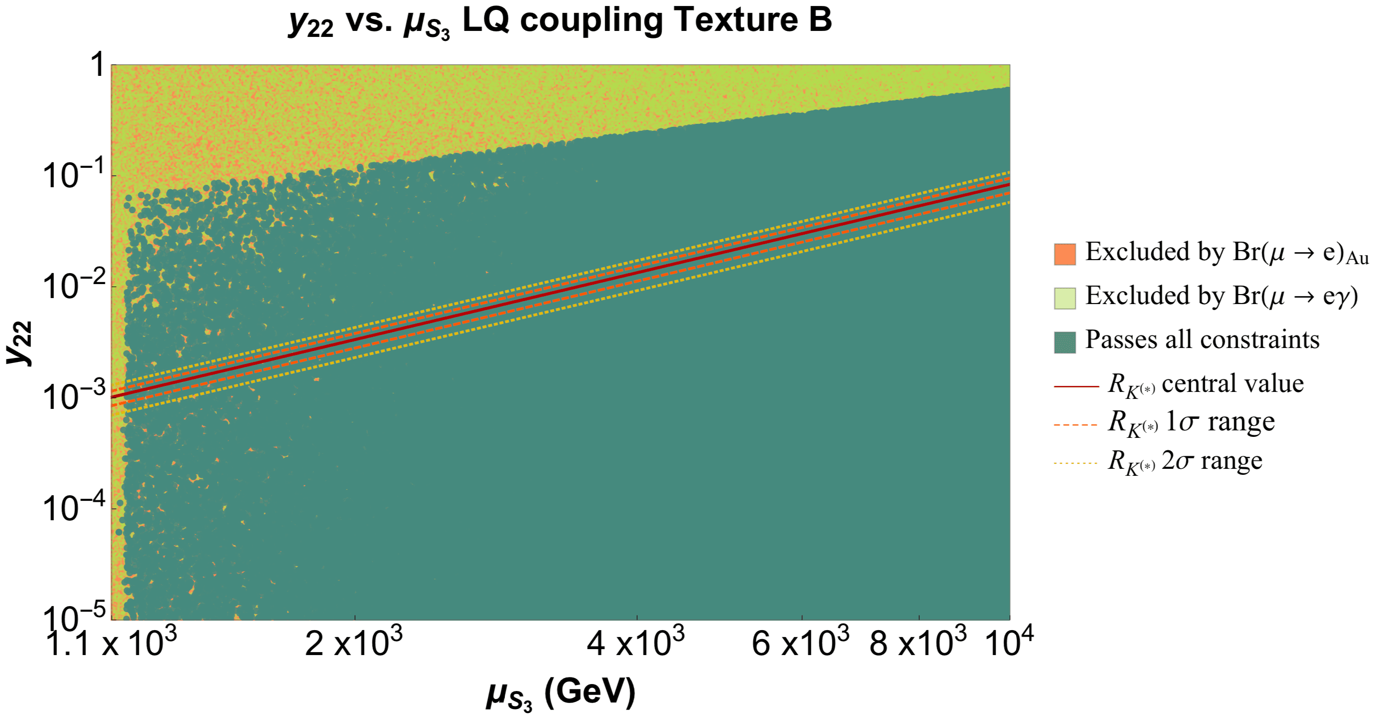
Figure 16: Indicative plot of the allowed parameter space in the $y_{22}$ vs. $\mu_{S_{3}}$ plane, for leptoquark coupling matrix Texture B. The red line indicates the central value needed to explain the $R_{K^{(*)}}$ anomalies with the dotted orange (yellow) lines indicating the $1(2)\sigma$ bounds. The orange region of the parameter space is constrained by $\text{Br}(\mu~{}\rightarrow~{}e)_{\text{Au}}$, the teal region is allowed; specifically it passes all constraints discussed in Section 3 as well as perturbativity constraints on the diquark coupling constants $z^{LL}_{1ij}$. The light green region, which in this plot has been superimposed on the orange, shows parameter space that is excluded by $\text{Br}(\mu~{}\rightarrow~{}e\gamma)$.

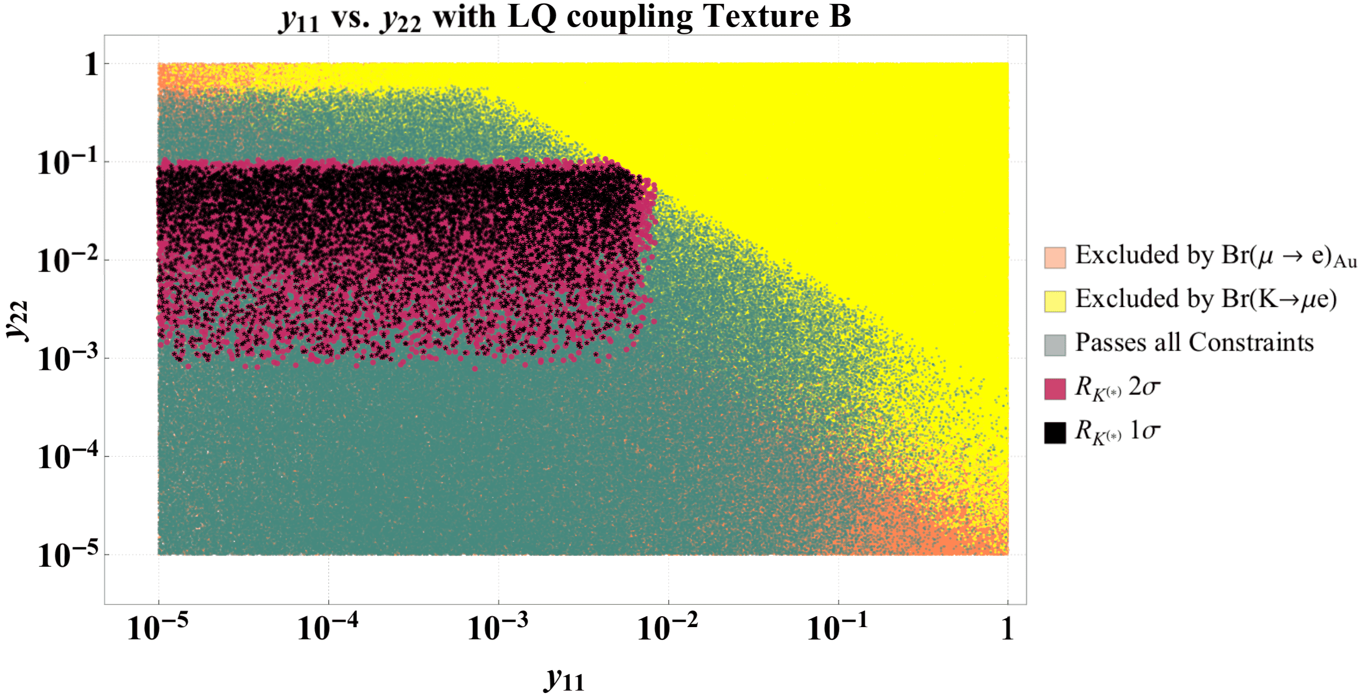
Figure 17: Indicative plot of the allowed parameter space in the $y_{22}$ vs. $y_{11}$ plane, for leptoquark coupling matrix Texture B. The yellow section is ruled out by $\text{Br}(K\rightarrow\mu e)$, the orange section is ruled out by $\text{Br}(\mu\rightarrow e)_{\text{Au}}$, while the teal region is allowed parameter space; specifically it passes all constraints discussed in Section 3 as well as perturbativity constraints on the diquark coupling constants $z^{LL}_{1ij}$.

4.3 Texture C

Finally, we consider leptoquark matrices of Texture C

$$\begin{split}y=\begin{pmatrix}y_{11}&y_{12}&\epsilon_{C}^{2}\\ y_{21}&y_{22}&\epsilon_{C}\\ \epsilon_{C}^{2}&1&1\end{pmatrix},\end{split}$$ (80)

where $\epsilon_{C}=10^{-1}$. When couplings between electrons or muons and third generation quarks are $\geq 10^{-2}$ there is a strong constraint on the leptoquark mass parameter coming from $\text{Br}(\mu\rightarrow e\gamma)$, which excludes parameter space less than $\mu_{S_{3}}\approx 4$ TeV, as seen in Figure 3.1.1. A similar bound in the $y_{22}$ versus $\mu_{S_{3}}$ slice of parameter space comes from the $\text{Br}(\mu\rightarrow e)_{Au}$ constraint. This can be seen in Figures 3.1.1 and 3.1.1. Constraints from $\text{Br}(K\rightarrow\mu e)$ still enforce that $y_{11}$ and $y_{22}$ cannot be simultaneously large, but it is the $\text{Br}(\mu\rightarrow e)_{\text{Au}}$ constraint that places a bound on the leptoquark couplings such that $y_{22}\lesssim 0.5$. The model can solve the $R_{K^{(*)}}$ anomalies to $1(2)\sigma$ for $\mu_{S_{3}}\lesssim 4$ TeV, $y_{11}\lesssim 10^{-2}$ and $10^{-2}\lesssim y_{11}\lesssim 10^{-1}$, as can be seen in black (pink) in Figures 3.1.1, 3.1.1 and 3.1.1. Unsurprisingly, regardless of the leptoquark coupling matrix texture, constraints from processes involving first generation quarks and leptons, expecially $\text{Br}(\mu\rightarrow e)$ provide the strongest bounds on the parameter space of our model and would also be the most promising signals.

Figure 18: Indicative plot of the allowed parameter space scans showing $\mu_{S_{3}}$ vs. $\text{Br}(\mu~{}\rightarrow~{}e)_{\text{Au}}$, for leptoquark coupling matrix Texture C. The purple line indicates the current $\text{Br}(\mu~{}\rightarrow~{}e)_{\text{Au}}$ cut-off, the dotted orange (yellow) line indicates the prospective cut-off from the Mu2e/COMET (PRISM) experiment. The light green region shows parameter space that is excluded by $\text{Br}(\mu~{}\rightarrow~{}e\gamma)$. The orange region of the parameter space is constrained by $\text{Br}(\mu~{}\rightarrow~{}e)_{\text{Au}}$, the teal region is allowed; specifically it passes all constraints discussed in Section 3 as well as perturbativity constraints on the diquark coupling constants $z^{LL}_{1ij}$. The black (pink) region solves the $R_{K^{(*)}}$ anomalies to $1(2)\sigma$.

Figure 19: Indicative plot of the allowed parameter space (in teal) in the $y_{22}$ vs. $\mu_{S_{3}}$ plane, for leptoquark coupling matrix Texture C. The red line indicates the central value needed to explain the $R_{K^{(*)}}$ anomalies with the purple (yellow) lines indicating the $1(2)\sigma$ bounds. Parameter space exluded by $\text{Br}(\mu\rightarrow e)$ is indicated in orange.

Figure 20: Indicative plot of the allowed parameter space in the $y_{22}$ vs. $y_{11}$ plane, for leptoquark coupling matrix Texture C. The yellow section is ruled out by $\text{Br}(K\rightarrow\mu e)$, the orange section is ruled out by $\text{Br}(\mu\rightarrow e)_{\text{Au}}$, while the teal region is allowed parameter space; specifically it passes all constraints discussed in Section 3 as well as perturbativity constraints on the diquark coupling constants $z^{LL}_{1ij}$.

Figure 21: Indicative plot of the allowed parameter space in the $y_{11}$ vs. $m_{S_{3}}$ plane, for leptoquark coupling matrix Texture C. The teal region shows allowed parameter space, while the orange region indicates parameter space excluded by constraints on $\text{Br}(\mu\rightarrow e)_{\text{Au}}$, while the yellow region show parameter space excluded by $\text{Br}(K\rightarrow\mu e)$. The black (pink) points indicate bounds on the parameters $y_{11}$ and $\mu_{S_{3}}$ needed to explain the $R_{K^{(*)}}$ anomalies to within $1(2)\sigma$.

5 Conclusion

There are a large number of candidate radiative Majorana neutrino mass models. The $\Delta L=2$ interactions responsible may be classified according to the dominant low-energy effective operators generated at tree-level from integrating out the massive exotic fields. The baryon-number conserving $\Delta L=2$ operators occur at odd mass dimension, and an extensive list has been compiled up to mass dimension 11 explodingOperators. An interesting question is: Beyond what mass dimension are phenomenologically viable models no longer possible? One generally expects that the higher the mass dimension, the higher also will be the number of vertices and loops in the neutrino self-energy graphs. Each additional vertex and loop contributes to additional suppression of the scale of neutrino mass, provided that the coupling constants at the vertices are small enough. There is also the prospect of suppression from powers of the ratio of electroweak scale to the new physics scale. At some point, the net suppression should become so strong that the $0.06$ eV lower bound on the neutrino mass scale cannot be generated for phenomenologically-acceptable exotic particle masses. Indeed, it has been argued that models constructed from opening up mass dimension 13 and higher operators are unlikely to be viable. Our findings in this paper, arrived at by a detailed examination of a specific model constructed from a dimension-11 operator, cast doubt on this tentative conclusion. The basic reason is evident from Equation 2: While there is a product of a few coupling constants in the numerator, and there is the $(1/16\pi^{2})^{2}$ two-loop suppression factor, the mass suppression is only $v^{2}/\Lambda$, so identical with that of the usual seesaw models. Formally, this is due to the neutrino mass diagram generating the same dimension-5 Weinberg operator as underpins the seesaw models, with the main difference being that it is generated at loop- rather than tree-level. Additional insertions of $v$ are often produced in radiative models from the need to use quark or charged-lepton mass insertions, but there is no such necessity in this model: the dominantly induced Weinberg-type operator is the standard one at dimension-5, rather than a higher-dimension generalisation obtained by multiplying by powers of $H^{\dagger}H$. At the level of the underlying renormalisable theory, one also observes that one of the contributing vertices in the numerator is a trilinear scalar coupling, thus having the dimension of mass, and most naturally set at the scale of the new physics. One possible source of suppression is thus absent. With order one dimensionless couplings, and the scalar trilinear coupling set at the new physics scale, the masses of the exotic scalars can be pushed as high as $10^{7}$ TeV. With the dimensionless couplings at $0.01$, so of fine-structure constant magnitude, the scale of new physics drops to the hundreds of GeV level. Hence, while the existence of new particles at the $1$-$100$ TeV scale explorable at current and proposed colliders is consistent with this model, it is not inevitable. From this perspective, models which require some of the couplings in the neutrino mass diagram to be standard-model Yukawa couplings (other than that of the top quark) are more experimentally relevant. From the model-building perspective, however, our analysis raises the prospect that some models based on tree-level UV completions of mass dimension 13 (and possibly even higher) operators might be viable. The specific model analysed in this paper, consisting of an isotriplet scalar leptoquark, an isosinglet diquark and a third exotic scalar multiplet that has no Yukawa interactions, successfully generates neutrino masses and mixings at two-loop level consistent with experimental bounds from a variety of processes, of which $\mu\to e$ conversion on nuclei proved to be the most stringent. It can also ameliorate the discrepancies between measurements and standard-model predictions for $R_{K^{(*)}}$ and the anomalous magnetic moment of the muon.