Minorization-Maximization-based Steepest Ascent for Large-scale Survival Analysis with Time-Varying Effects: Application to the National Kidney Transplant Dataset

Abstract

The time-varying effects model is a flexible and powerful tool for modeling the dynamic changes of covariate effects. However, in survival analysis, its computational burden increases quickly as the number of sample sizes or predictors grows. Traditional methods that perform well for moderate sample sizes and low-dimensional data do not scale to massive data. Analysis of national kidney transplant data with a massive sample size and large number of predictors defy any existing statistical methods and software. In view of these difficulties, we propose a Minorization-Maximization-based steepest ascent procedure for estimating the time-varying effects. Leveraging the block structure formed by the basis expansions, the proposed procedure iteratively updates the optimal block-wise direction along which the approximate increase in the log-partial likelihood is maximized. The resulting estimates ensure the ascent property and serve as refinements of the previous step. The performance of the proposed method is examined by simulations and applications to the analysis of national kidney transplant data.

Keywords Kidney transplant  $\cdot$ Survival analysis  $\cdot$ Steepest ascent  $\cdot$ Time-varying effects

1 Introduction

End-stage renal disease (ESRD) is one of the most deadly and costly diseases in the United States. Kidney transplantation is the preferred treatment for ESRD. However, despite aggressive efforts to increase the number of kidney donors, the demand far exceeds the supply, with fewer than $15\%$ of eligible patients likely to receive a transplant [36]. To optimize treatment strategies for ESRD patients, an important aspect is to understand why the outcome is worse for certain patients. Thus, there is urgent need to accurately identify risk factors associated with post-transplant mortality.

For this purpose, the proportional hazards model [5] has been widely employed. However, the Cox model assumes the covariate effects are constant over time, which is often violated due to the complex relationships between baseline conditions and post-treatment outcomes. One example is obesity, generally viewed as a risk factor for mortality; however, previous studies [6] showed improved survival in obese kidney dialysis patients, which has been labeled as reverse epidemiology. One possible explanation is that obesity has a protective effect in the short run (Figure 1a), but becomes a risk factor after long-term exposure. Another example is core muscle size. Englesbe et al. [7] found that large core muscle size has a strong protective effect in the short term after surgery, with a weakening association over time (Figure 1b). In contrast, the constant estimate provided by the Cox model is close to zero. Thus, accounting for time-varying effects provides valuable clinical information that could be obscured otherwise.

Figure 1: Example time-varying effects in clinical studies. The solid lines are B-spline based estimates. The constant estimates are provided by the Cox model.

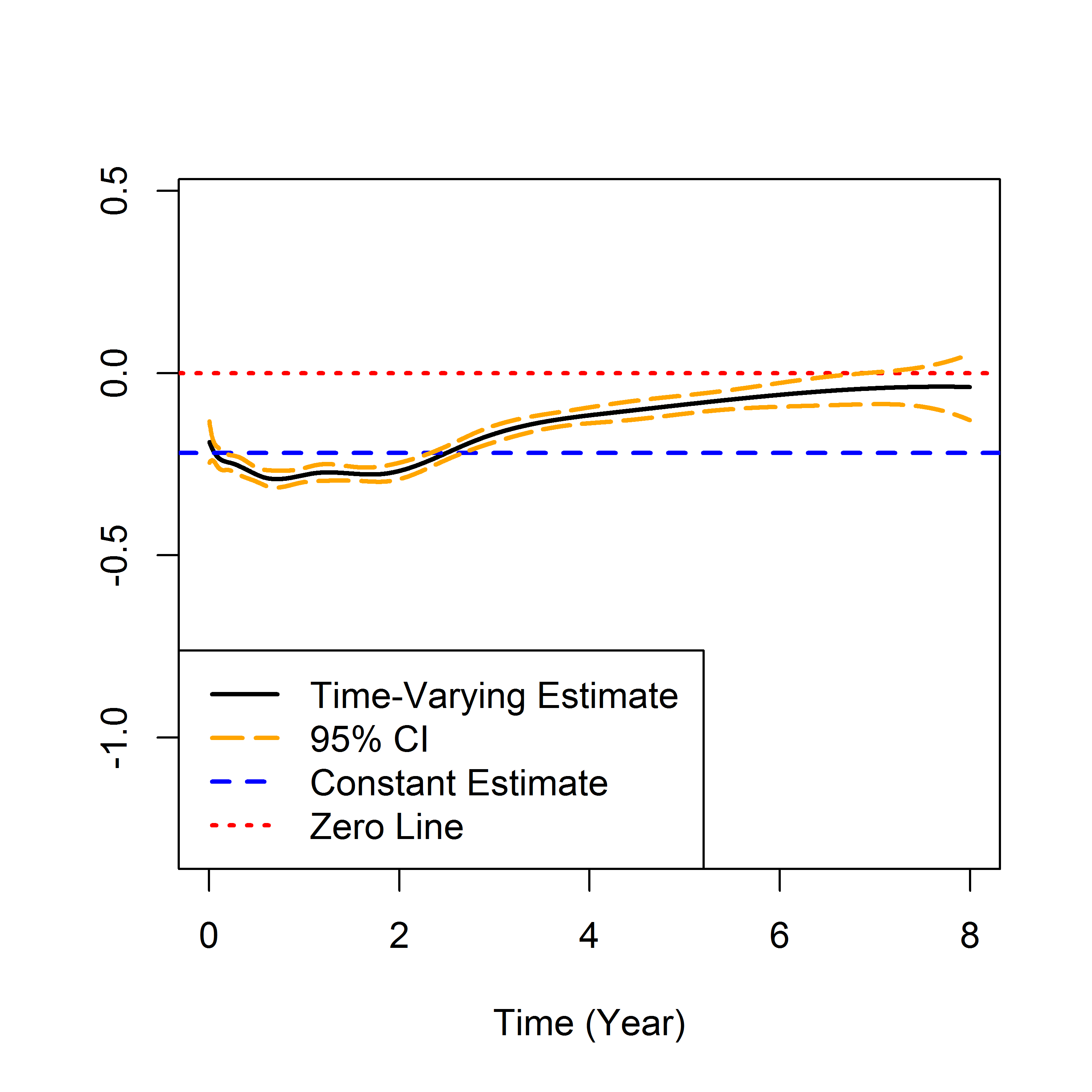
(a) Obesity for Dialysis Outcomes

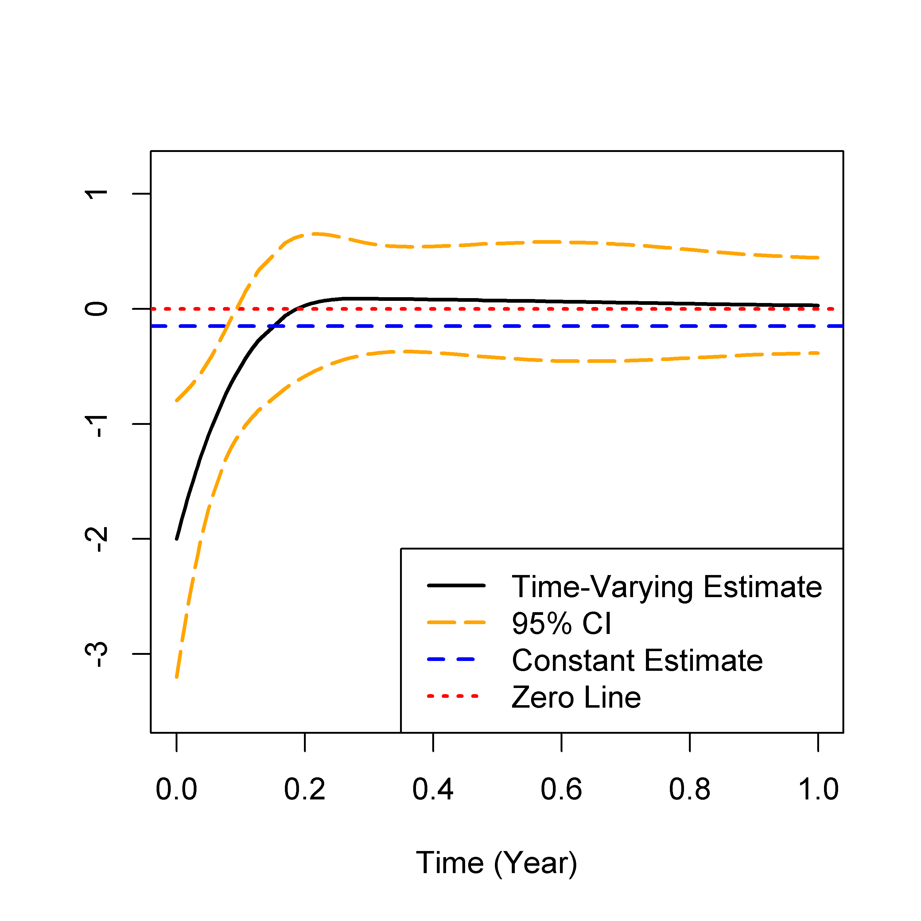
(b) Core Muscle Size for Surgical Outcomes

Figure 2: Computation time and estimation error.

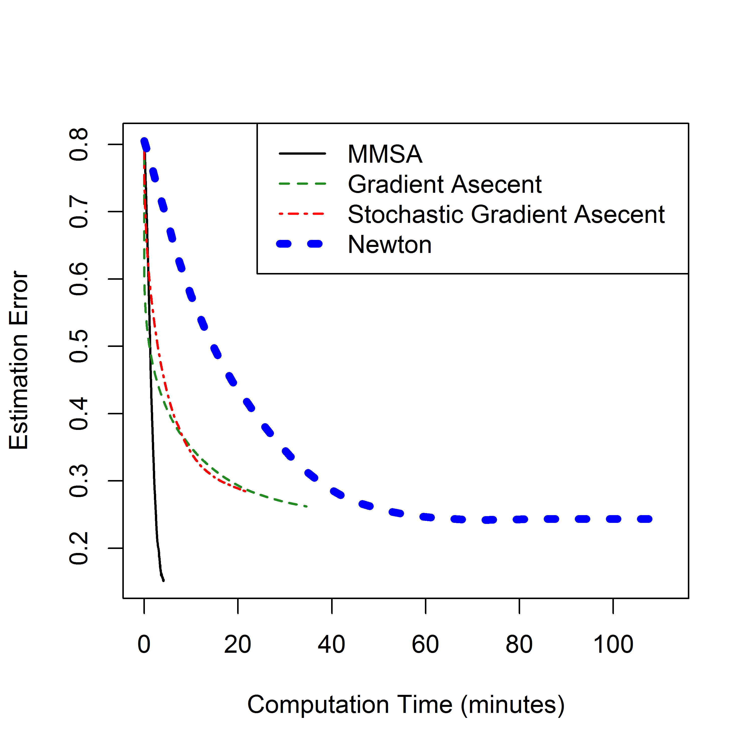
(a) P=5

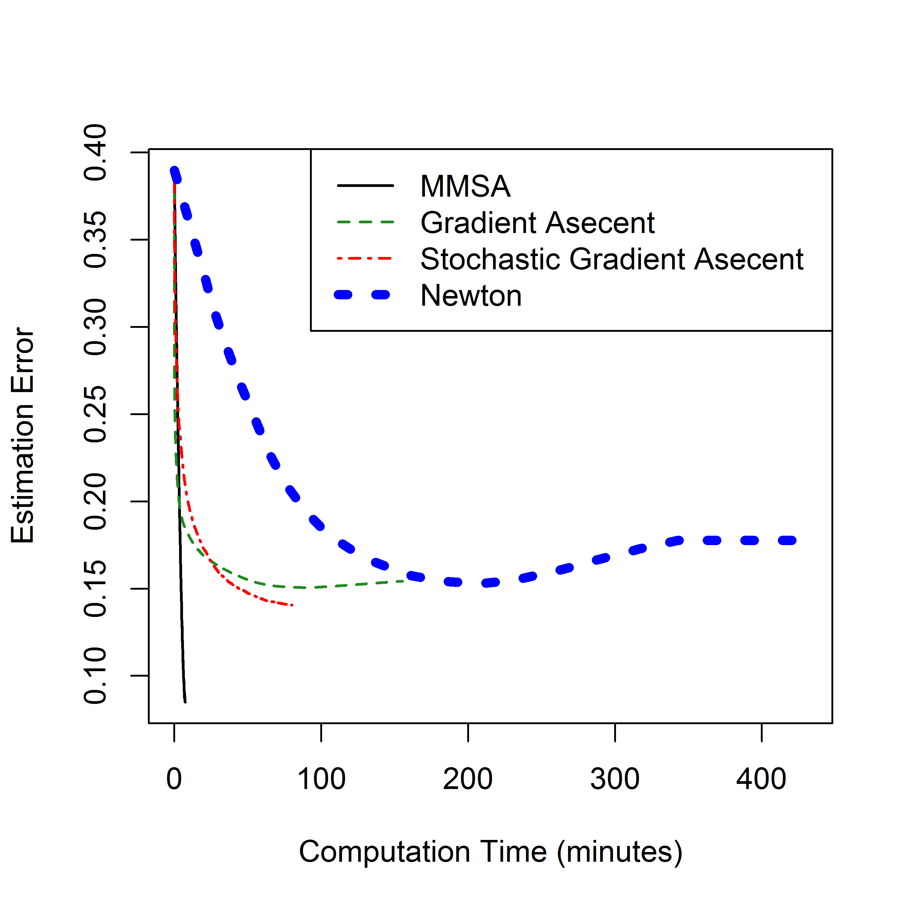
(b) P=20

To extend the standard Cox model, time-varying effects have been widely studied. Zucker and Karr [45] utilized a penalized partial likelihood approach and proposed nonparametric estimation of the time-varying effects. A specialized algorithm for this problem was then provided by Hastie and Tibshirani [18]. Alternatively, Gray [15, 16] proposed using fixed knots spline functions. Kernel-based partial likelihood approaches have also been developed [37, 27]. Some recent studies [23, 42] have proposed selection of time-varying effects using penalized methods such as adaptive Lasso [43, 44]. Xiao, Lu, and Zhang [41] combined the ideas of local polynomial smoothing and group nonnegative garrote to achieve these goals. He et al. [19] considered a frailty model with time-varying effects.

While successful, these methods present challenges for large-scale studies. To estimate time-varying effects in survival analysis, datasets are usually expanded in a repeated measurement format, where the time is divided into small intervals of a single event. Within each interval, the covariate values and outcomes for at-risk subjects are stacked to a large working dataset, which becomes infeasible for large sample sizes. To avoid the data expansion, a routine based on Kronecker product has been suggested [31]. However, in our motivating setting, the pertinent analysis file is extremely large because there are over 300,000 transplant patients. The algorithm, which involves iterative computation and inversion of the observed information matrix, can easily overwhelms a computer with an 32G memory.

Moreover, to estimate time-varying effects, one may represent the coefficients using basis expansions such as B-splines. Thus, the parameter vector carries block structures, for which extra parameters are created and the computational burden increases quickly as the number of predictors grows. In particular, the kidney transplant database includes more than 160 predictors and many of which are comorbidities with rare frequencies. The inversion of the observed information matrix leads to unstable estimations, especially in the right-tail of the follow-up period, because the data tends to be sparse there due to the censoring.

To exemplify this issue, we conducted a simulated example to compare the proposed method (termed MMSA) with Newton approach, gradient ascent, and stochastic gradient ascent with step size determined by Adagrad algorithm [35]. Detailed simulation set-up is provided in Setting 2 of Section 3. Figure 2 compares the computation times and average estimation errors. When the number of parameters is large, the Newton approach introduces large estimation biases. Gradient-based methods also face serious limitations by overlooking useful information from the Hessian matrix. In contrast, the proposed approach is computationally efficient and substantially improves the estimation error.

Our proposed solution is motivated by boosting [9], which was originally introduced for classifying binary outcomes. Breiman [2] formulated boosting as a gradient descent approach with a special loss function. Mason et al. [28] developed a related algorithm, which was mainly acknowledged in the machine learning community. Friedman, Hastie and Tibshirani [10] and Friedman [11] laid out a gradient boosting framework to handle a variety of loss functions. Bühlmann and Yu [3] proposed a novel component-wise boosting procedure based on $\ell_{2}$ loss functions, and Bühlmann and Yu [4] further demonstrated that the component-wise procedure works well in high-dimensional linear models. Wolfson [40] developed a modification of gradient boosting under the estimation equation settings.

While demonstrating promising performance for proportional hazards model [21], as illustrated by Hofner, Hothorn, and Kneib [22], conventional gradient boosting cannot accommodate time-varying effects in survival analysis. Alternatively, likelihood-based boosting was considered [22]. However, this approach is computationally intensive, preventing its use in large-scale settings.

To fill in these gaps, we propose a new steepest ascent procedure based on a Minorization-Maximization (MM) algorithm [26]. Our proposed approach converts a difficult optimization problem into a sequence of simpler ones. Simplicity is achieved by avoiding iterative computation and inversion of large-scale observed information matrix, which is especially important for large-scale analysis. Leveraging the block structure formed by the basis expansions, the proposed procedure iteratively updates the optimal block-wise direction along which the directional derivative is maximized and, hence, the approximate increase in log-partial likelihood is greatest. The resulting estimates ensure the ascent property and serve as refinements of the previous step. As exemplified in Figure 2, our procedure provides well-behaved results, achieving less estimation error and improved computational efficiency.

2 Method

2.1 Model

In our motivating example, patients came from multiple transplant centers. In the absence of adjustment for center effects, the estimation of covariate effects may be substantially biased [25]. To avoid this issue, we adopt a stratified model with center-specific baseline hazards. Another advantage of using a stratified model is that it greatly reduces the calculations across the partial likelihood contributions, which is especially important for the large-scale data exemplified in our study.

Let $D_{ij}$ denote the death time and $C_{ij}$ be the censoring time for patient $i$ in center $j$, $i=1,\ldots,n_{j}$, and $j=1,\ldots,J$. Here $n_{j}$ is the sample size in center $j$, and $J$ is the number of centers. The observed time is denoted as $T_{ij}=\min\{D_{ij},C_{ij}\}$, and the death indicator is given by $\delta_{ij}=I(D_{ij}<C_{ij})$. Let $\textbf{X}_{ij}=(X_{ij1},\ldots,X_{ijP})^{T}$ be a $P$-dimensional covariate vector. We assume that, upon conditioning on $\textbf{X}_{ij}$, $D_{ij}$ is independently censored by $C_{ij}$. Consider a center-specific hazard function

$$\lambda(t|\mathbf{X}_{ij})=\lambda_{0j}(t)\exp(\mathbf{X}_{ij}^{T}{\boldsymbol{\beta}}(t)),$$

where $\lambda_{0j}(t)$ is the center-specific baseline hazard. To estimate the time-varying coefficients ${\boldsymbol{\beta}}(t)=(\beta_{1}(t),\ldots,\beta_{P}(t))$, we span $\boldsymbol{\beta}(\cdot)$ by a set of B-splines on a fixed grid of knots:

$$\beta_{p}(t)=\boldsymbol{\theta}_{p}^{T}\mathbf{B}(t)=\sum_{k=1}^{K}\theta_{pk}B_{k}(t),~{}~{}p=1,\ldots,P,$$

where $\mathbf{B}(t)=(B_{1}(t),\ldots,B_{K}(t))^{T}$ forms a basis, and $\boldsymbol{\theta}_{p}=(\theta_{p1},\ldots,\theta_{pK})^{T}$ is a vector of coefficients with $\theta_{pk}$ being the coefficient for the $k$-th basis of the $p$-th covariate. Considering a length-$PK$ parameter vector $\boldsymbol{\theta}=vec(\boldsymbol{\Theta})$, the vectorization of the coefficient matrix $\boldsymbol{\Theta}=(\boldsymbol{\theta}_{1},\ldots,\boldsymbol{\theta}_{P})^{T}$ by row, the log-partial likelihood function is

$$\ell(\boldsymbol{\theta})=\sum_{j=1}^{J}\sum_{i=1}^{n_{j}}\delta_{ij}\left[\mathbf{X}_{ij}^{T}\boldsymbol{\Theta}\mathbf{B}(T_{ij})-\log\left\{\sum_{i^{\prime}\in R_{ij}}\exp\left(\mathbf{X}_{i^{\prime}j}^{T}\boldsymbol{\Theta}\mathbf{B}(T_{ij})\right)\right\}\right],$$ (1)

where $R_{ij}=\{i^{\prime}:1\leq i^{\prime}\leq n_{j},~{}T_{i^{\prime}j}\geq T_{ij}\}$ is the center-specific at-risk set. For small-sized problems, maximizing (1) can be achieved by a Newton’s approach, which, however, becomes impractical for large-scale problems.

2.2 Motivation

To improve computational efficiency and numerical stability, we consider a first-order approximation of $\ell(\boldsymbol{\theta})$ around the current estimate $\widehat{\boldsymbol{\theta}}$:

$$\ell(\boldsymbol{\widehat{\theta}}+\alpha\boldsymbol{\mu})=\ell(\boldsymbol{\widehat{\theta}})+\alpha\triangledown\ell(\widehat{\boldsymbol{\theta}})^{T}\boldsymbol{\mu}+o(\alpha),$$

where $\boldsymbol{\mu}$ is the update direction of $\boldsymbol{\theta}$, $\alpha$ is a small positive value, $\triangledown\ell(\widehat{\boldsymbol{\theta}})$ is the gradient, and the term $\triangledown\ell(\widehat{\boldsymbol{\theta}})^{T}\boldsymbol{\mu}$ is the directional derivative along the direction $\boldsymbol{\mu}$:

$$\triangledown\ell(\widehat{\boldsymbol{\theta}})^{T}\boldsymbol{\mu}=\frac{\partial}{\partial\alpha}\ell(\boldsymbol{\widehat{\theta}}+\alpha\boldsymbol{\mu})\bigg{\rvert}_{\alpha=0}=\lim_{\alpha\rightarrow 0}\frac{\ell(\boldsymbol{\widehat{\theta}}+\alpha\boldsymbol{\mu})-\ell(\boldsymbol{\widehat{\theta}})}{\alpha}.$$

If $\triangledown\ell(\widehat{\boldsymbol{\theta}})^{T}\boldsymbol{\mu}>0$, $\boldsymbol{\mu}$ is an ascent direction driving $\ell(\boldsymbol{\theta})$ uphill. Intuitively, we wish to identify a unit norm update direction such that $\ell(\boldsymbol{\widehat{\theta}}+\alpha\boldsymbol{\mu})$ ascends most rapidly. This motivates a steepest ascent direction that maximizes the direction derivative

$$\boldsymbol{\mu}^{\star}=\operatornamewithlimits{argmax}_{\boldsymbol{\mu}}\{\triangledown\ell(\widehat{\boldsymbol{\theta}})^{T}\boldsymbol{\mu}~{}\big{|}~{}||\boldsymbol{\mu}||_{\dagger}=1\},$$ (2)

where $||\cdot||_{\dagger}$ is a norm on $\mathbb{R}^{PK}$.

2.3 Example Norms

The choice of norm $||\boldsymbol{\mu}||_{\dagger}$ plays a critical role in the performance of (2). If we choose a $\ell_{2}$ norm, the corresponding dual norm [1] is the $\ell_{2}$ norm itself, which leads to a gradient ascent method. As illustrated in Figure 2, its convergence can be very slow. Alternatively, if we consider a $\ell_{1}$ norm, the corresponding dual norm is the $\ell_{\infty}$ norm, which leads to a coordinate-wise gradient boosting procedure. However, this approach is not suitable for our motivating setting, in which the parameter vector carries a group structure formed by representing the time-varying coefficients using basis expansions.

2.4 Block-Wise Steepest Ascent

To leverage the block structure of our parameter vectors, we consider a $\ell_{1}$/quadratic norm,

$$||\boldsymbol{\mu}||_{\dagger}=\sum_{p=1}^{P}\big{|}\big{|}\boldsymbol{\mu}_{p}\big{|}\big{|}_{\mathbf{H}_{p}(\boldsymbol{\widehat{\theta}})},~{}~{}\mbox{where}~{}~{}||\boldsymbol{\mu}_{p}||_{\mathbf{H}_{p}(\boldsymbol{\widehat{\theta}})}=\left(\boldsymbol{\mu}_{p}^{T}\mathbf{H}_{p}(\boldsymbol{\widehat{\theta}})\boldsymbol{\mu}_{p}\right)^{1/2}.$$ (3)

Here $\boldsymbol{\mu}_{p}$ is a $K$-dimensional vector corresponding to the $p$-th block of $\boldsymbol{\mu}$, and $\mathbf{H}_{p}(\boldsymbol{\widehat{\theta}})$ is a $K\times K$-dimensional matrix. Specifically, for $p=1,\ldots,P$, we choose

$$\mathbf{H}_{p}(\widehat{\boldsymbol{\theta}})=-\left(\triangledown\ell(\widehat{\boldsymbol{\theta}})_{p}^{T}(-\triangledown^{2}\ell(\widehat{\boldsymbol{\theta}})_{p})^{-1}\triangledown\ell(\widehat{\boldsymbol{\theta}})_{p}\right)\triangledown^{2}\ell(\widehat{\boldsymbol{\theta}})_{p},$$

where $\triangledown\ell(\widehat{\boldsymbol{\theta}})_{p}$ is a $K$-dimensional gradient vector and $\triangledown^{2}\ell(\widehat{\boldsymbol{\theta}})_{p}$ is the $p$-th block diagonal of the Hessian matrix, corresponding to the $p$-th variable. The scalar $\triangledown\ell(\widehat{\boldsymbol{\theta}})_{p}^{T}(-\triangledown^{2}\ell(\widehat{\boldsymbol{\theta}})_{p})^{-1}\triangledown\ell(\widehat{\boldsymbol{\theta}})_{p}$ plays a role as a normalization factor. Apply the Cauchy-Schwarz inequality,

$$\triangledown\ell(\widehat{\boldsymbol{\theta}})^{T}\boldsymbol{\mu}\leq\sum_{p=1}^{P}\big{|}\big{|}\triangledown\ell(\widehat{\boldsymbol{\theta}})_{p}\big{|}\big{|}_{\mathbf{H}_{p}^{-1}(\boldsymbol{\widehat{\theta}})}\big{|}\big{|}\boldsymbol{\mu}_{p}\big{|}\big{|}_{\mathbf{H}_{p}(\boldsymbol{\widehat{\theta}})}\leq\max_{p}\left(\big{|}\big{|}\triangledown\ell(\widehat{\boldsymbol{\theta}})_{p}\big{|}\big{|}_{\mathbf{H}_{p}^{-1}(\boldsymbol{\widehat{\theta}})}\right)\sum_{p=1}^{P}\big{|}\big{|}\boldsymbol{\mu}_{p}\big{|}\big{|}_{\mathbf{H}_{p}(\boldsymbol{\widehat{\theta}})}.$$

Thus, the dual norm of a $\ell_{1}$/quadratic norm is the $\ell_{\infty}$/quadratic norm. The resulting $\boldsymbol{\mu}^{\star}$ is the normalized direction in the unit ball of $\ell_{1}$/quadratic norm that extends farthest in the direction of gradient $\triangledown\ell(\widehat{\boldsymbol{\theta}})$, and is given by

$$\boldsymbol{\mu}^{\star}=(0,\ldots,0,\widetilde{\boldsymbol{\mu}}_{p^{\star}}^{T},0,\ldots,0)^{T},$$ (4)

where $p^{\star}$ is the optimal block maximizing the block-wise directional derivative

$$p^{\star}=\operatornamewithlimits{argmax}_{p}\nabla\ell(\boldsymbol{\widehat{\theta}})_{p}^{T}\widetilde{\boldsymbol{\mu}}_{p},$$ (5)

with $\widetilde{\boldsymbol{\mu}}_{p}$ being a $K$-dimensional update vector corresponding to the $p$-th variable

$$\widetilde{\boldsymbol{\mu}}_{p}=\left(\mathbf{H}_{p}(\widehat{\boldsymbol{\theta}})\right)^{-1}\triangledown\ell(\widehat{\boldsymbol{\theta}})_{p}.$$ (6)

This leads to a Minorization-Maximization-based steepest ascent procedure that iteratively pursues the optimal block-wise direction maximizing the directional derivative.

2.5 Minorization Step

In the minorization step, the $\ell_{1}$/quadratic norm considered in (3) leads to the following minority surrogate function

$$g(\boldsymbol{\theta}|\widehat{\boldsymbol{\theta}})=\ell(\widehat{\boldsymbol{\theta}})+\triangledown\ell(\widehat{\boldsymbol{\theta}})^{T}(\boldsymbol{\theta}-\widehat{\boldsymbol{\theta}})-\frac{1}{2\nu}(\boldsymbol{\theta}-\widehat{\boldsymbol{\theta}})^{T}\mathbf{H}(\widehat{\boldsymbol{\theta}})(\boldsymbol{\theta}-\widehat{\boldsymbol{\theta}}),$$

where $\nu$ is a small positive value to be specified. Here $\mathbf{H}(\widehat{\boldsymbol{\theta}})$ is a block-diagonal matrix, where the blocks correspond to the basis expansions for each variable. In particular,

$$\mathbf{H}(\widehat{\boldsymbol{\theta}})=\begin{bmatrix}\mathbf{H}_{1}(\widehat{\boldsymbol{\theta}})&0&\dots&0\\ 0&\mathbf{H}_{2}(\widehat{\boldsymbol{\theta}})&\dots&0\\ \vdots&\vdots&\ddots&\vdots\\ 0&0&\dots&\mathbf{H}_{P}(\widehat{\boldsymbol{\theta}})\end{bmatrix}$$

with all non-block-diagonal elements being zeros. It is obvious that $g(\boldsymbol{\widehat{\theta}}|\boldsymbol{\widehat{\theta}})=\ell(\boldsymbol{\widehat{\theta}})$. Proposition 1 in Section 2.7 shows that, with a suitable choice of $\nu$, $g(\boldsymbol{\theta}|\widehat{\boldsymbol{\theta}})\leq\ell(\boldsymbol{\theta})$ for all $\boldsymbol{\theta}$.

2.6 Maximization Step

In the maximization step, the block-wise update in (5) and (6) maximizes $g(\boldsymbol{\theta}|\boldsymbol{\widehat{\theta}})$ subject to a constraint that only one variable is updated at each iteration. The resulting estimates of $\boldsymbol{\theta}$ ensure the ascent property and thus serve as refinements of the previous step. We summarize the proposed algorithm as follows:

Algorithm (MMSA)

1. Initialize $\boldsymbol{\widehat{\theta}}^{(0)}=\textbf{0}$. For $m=1,2,3,\ldots$, identify $p^{\star}$ as in (5).

2. Update the estimate by

   $$\boldsymbol{\widehat{\theta}}^{(m)}_{p^{\star}}=\boldsymbol{\widehat{\theta}}^{(m-1)}_{p^{\star}}+\nu~{}\widetilde{\boldsymbol{\mu}}_{p^{\star}}.$$

3. The iteration continues until $\max_{p}\nabla\ell(\boldsymbol{\widehat{\theta}}^{(m-1)})_{p}^{T}\widetilde{\boldsymbol{\mu}}_{p}$ or the relative change in the log-partial likelihood is less than a convergence threshold (e.g. $10^{-6}$).

Remark 1: The proposed MMSA is a block-wise procedure. At each iteration, only one variable is updated. The corresponding block-wise update direction maximizes the block-wise directional derivative, $\nabla\ell(\boldsymbol{\widehat{\theta}}^{(m-1)})_{p}^{T}\widetilde{\boldsymbol{\mu}}_{p}$, which ranks the importance of each predictor and measures how fast the log-partial likelihood would increase by including each predictor.

Remark 2: The proposed algorithm converts a difficult optimization problem into a simpler surrogate function. Simplicity is achieved by avoiding iterative computation and inversion of large-scale observed information matrix. Numerical results show that the proposed algorithm provides sufficient and rapid updates, achieving much computational efficiency.

Remark 3: The learning rate, $\nu$, can be chosen to be a small positive value, e.g. 0.05. Further clarification for the choice of $\nu$ is provided in Section 2.7.

Remark 4: To further improve computational efficiency, a stochastic procedure [12] can be applied. At each iteration, we sample a fraction $\eta$ (e.g. $\eta=0.2$) of the observations (without replacement), and estimate the update using the subsample. Not only does the sampling reduce the computing time (which is especially important for large-scale data), but also it improves estimation performance.

Figure 3: Average estimated coefficients across various MMSA and gradient ascent (termed gradient) iterations; $\beta_{2}(t)=sin3(\pi t/4)$ and $\beta_{4}(t)=-(t/3)^{2}\exp(t/2)$ are time-varying effects; based on 100 simulation replicates; m: number of iterations.

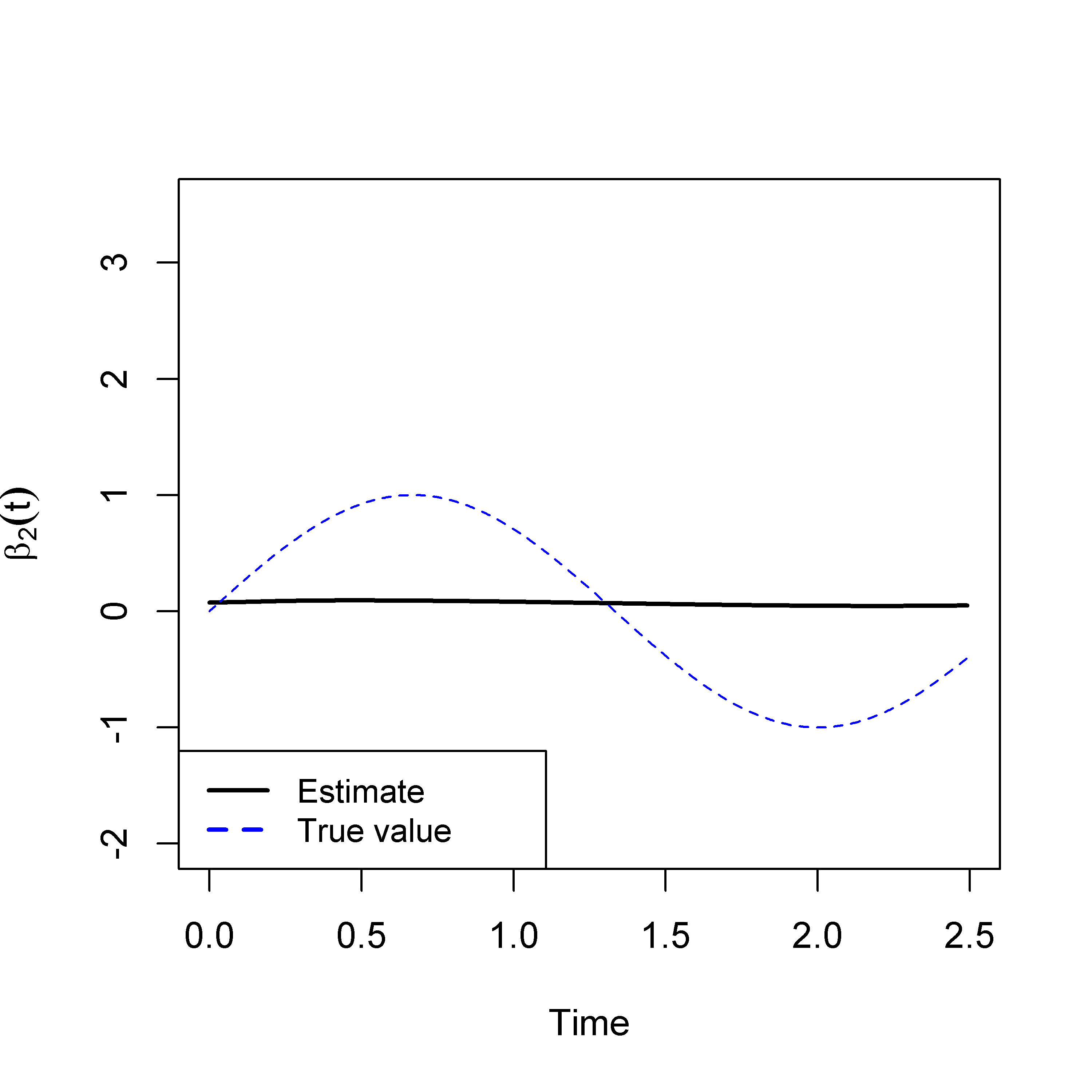
(a) MMSA: m=500

(b) MMSA: m=1,000

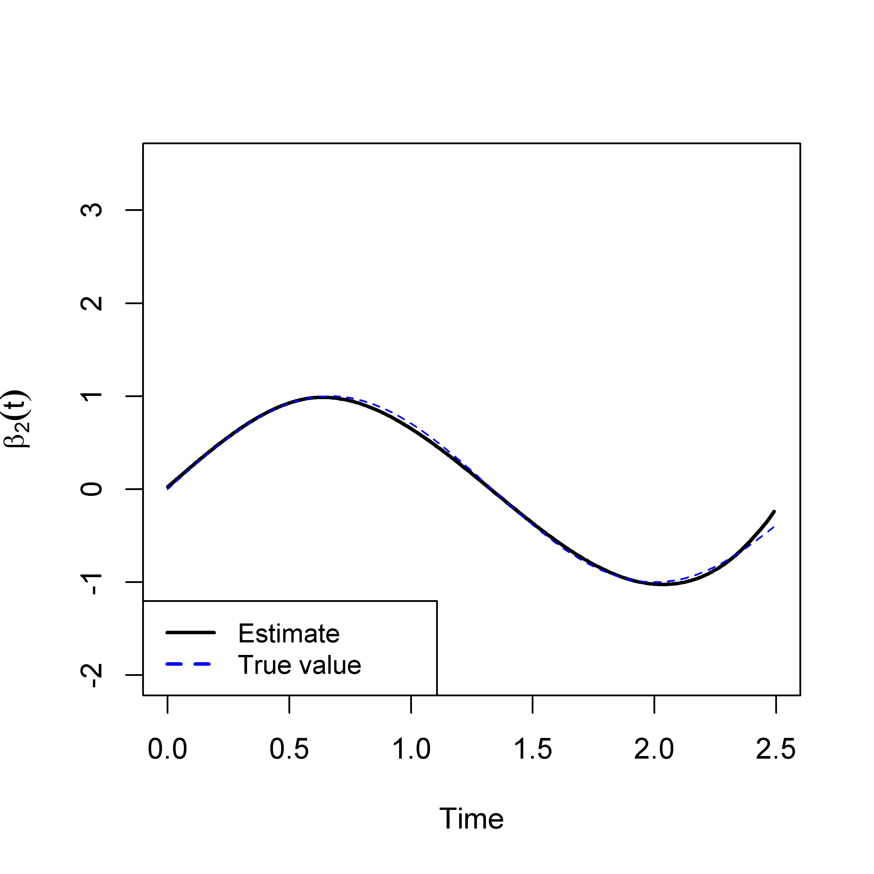
(c) MMSA: m=3,000

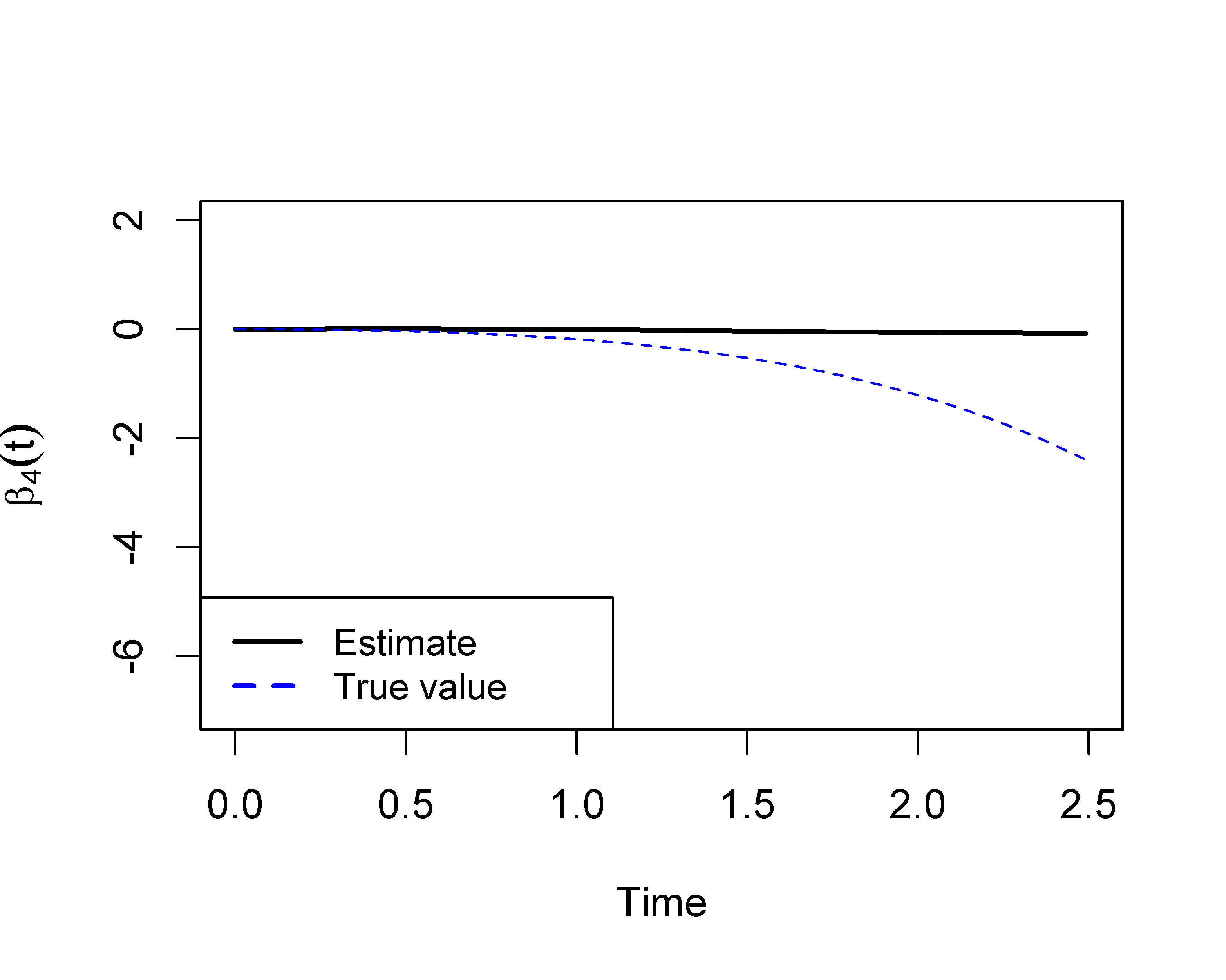
(d) MMSA: m=500

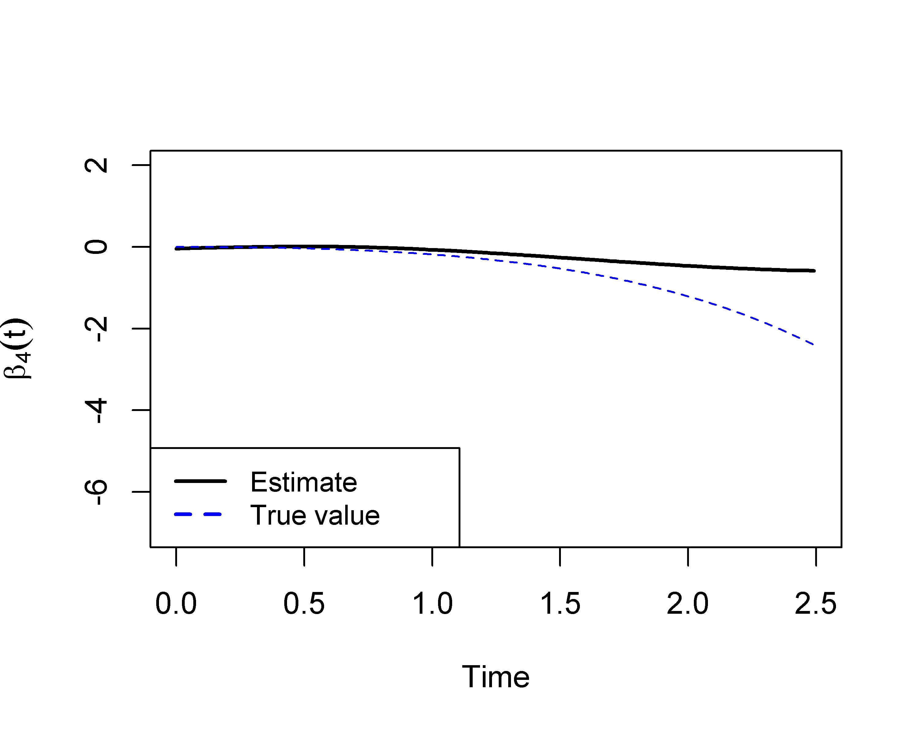
(e) MMSA: m=1,000

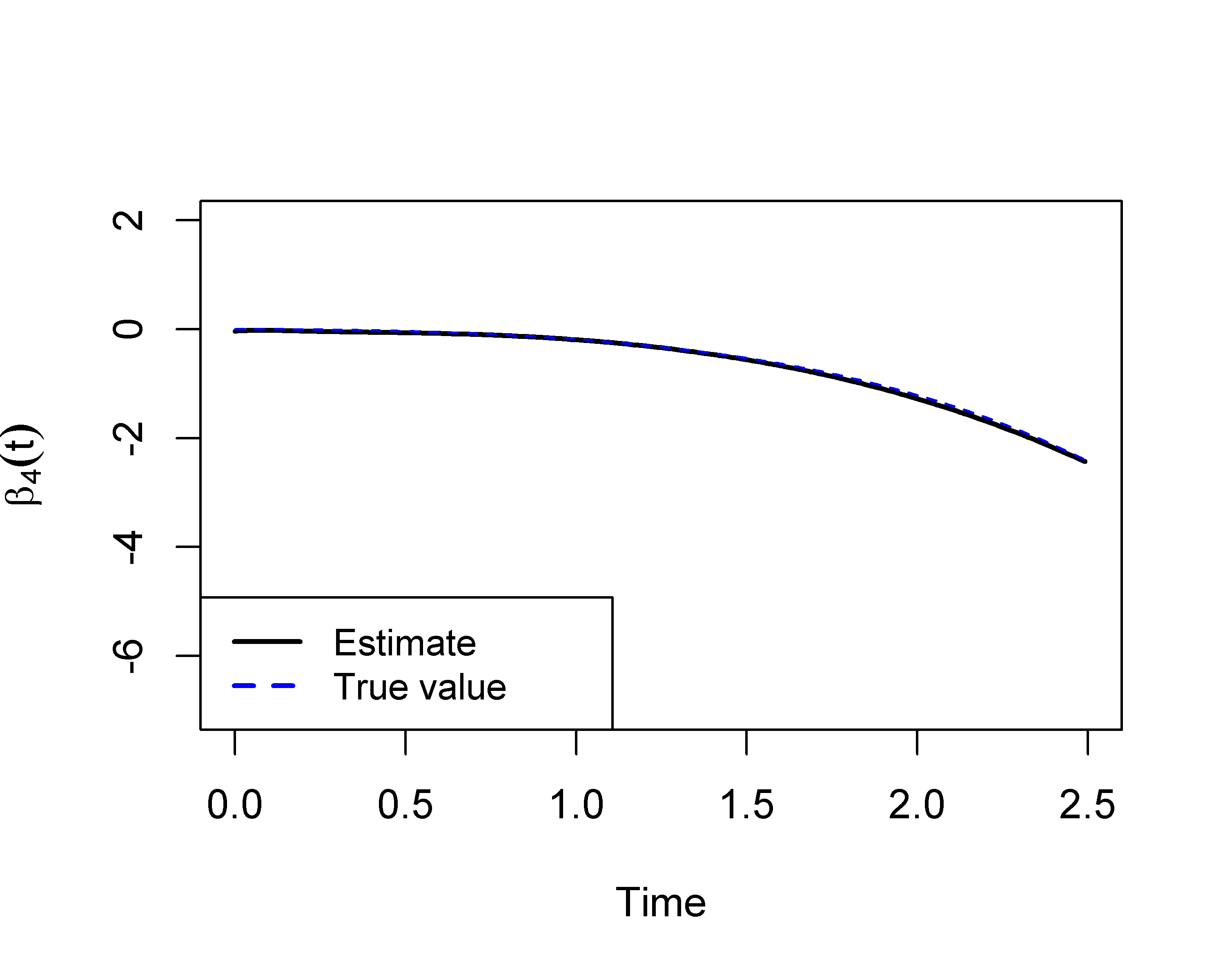
(f) MMSA: m=3,000

(g) Gradient: m=500

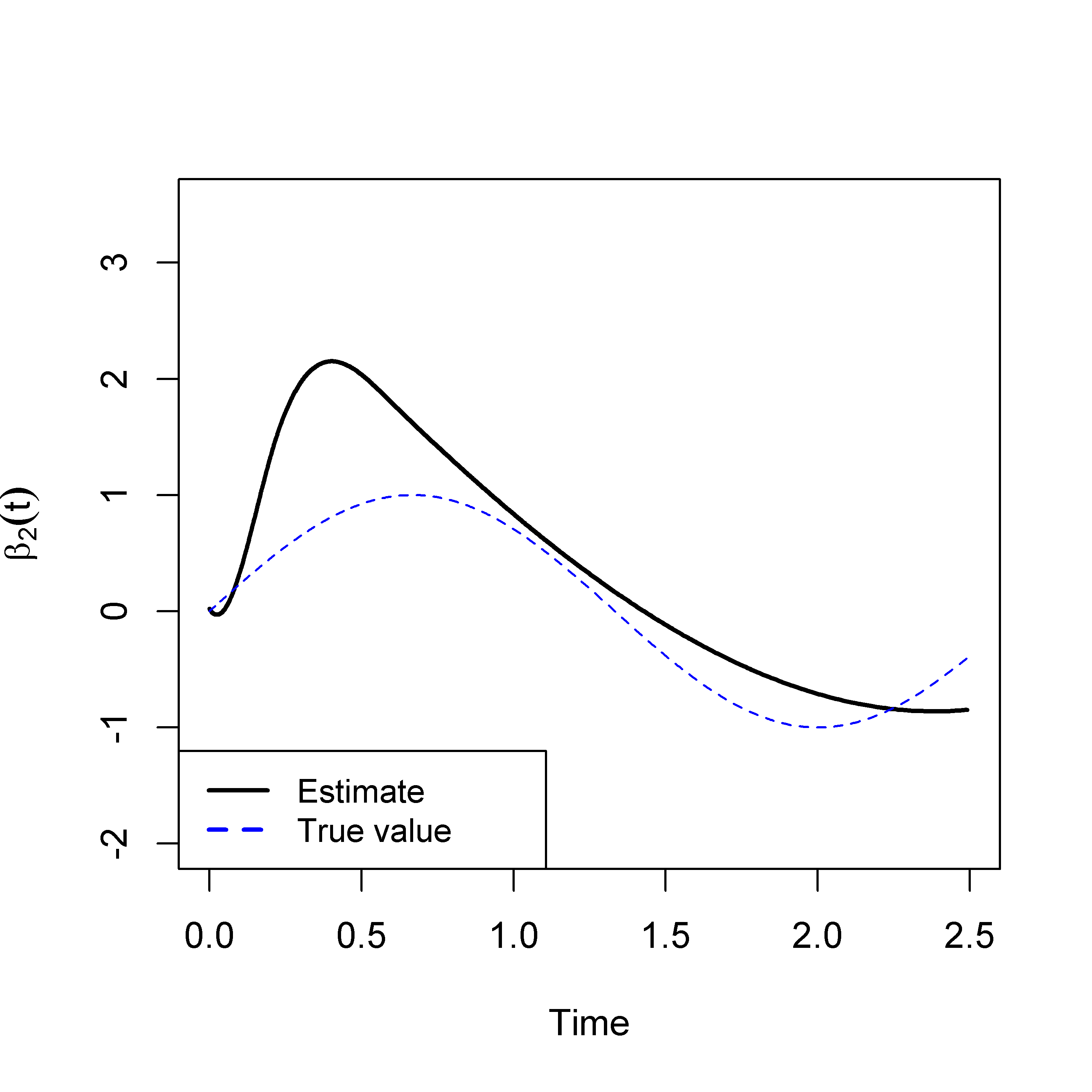
(h) Gradient: m=1,000

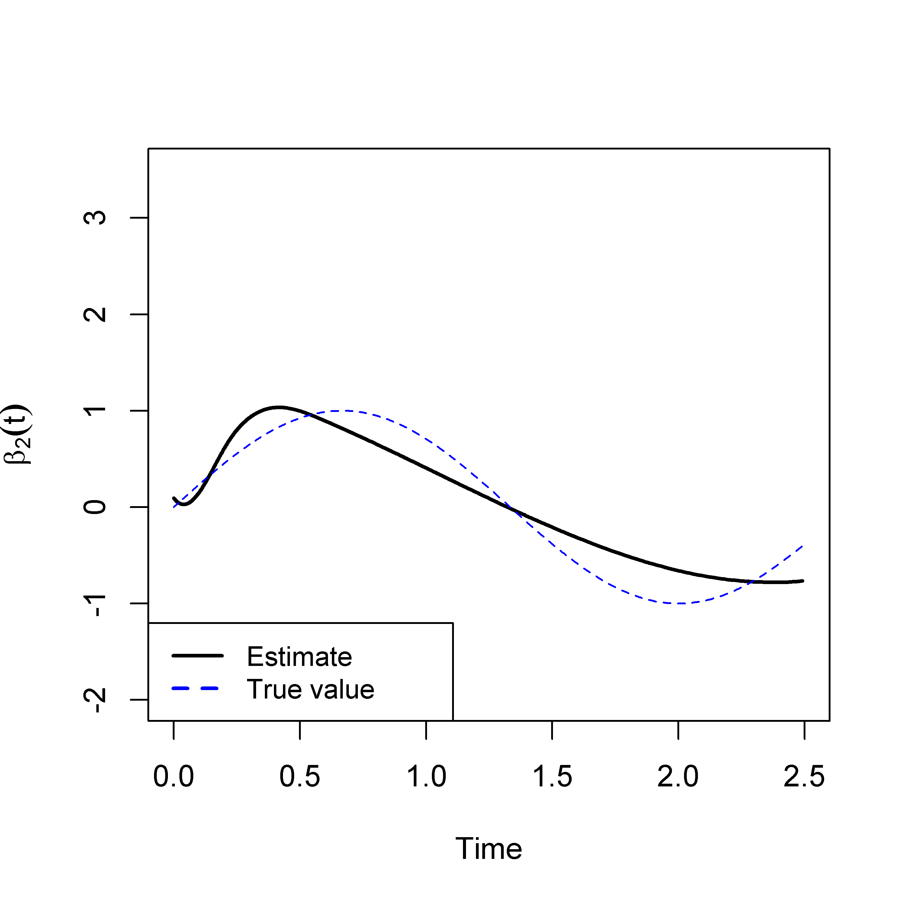
(i) Gradient: m=3,000

(j) Gradient: m=500

(k) Gradient: m=1,000

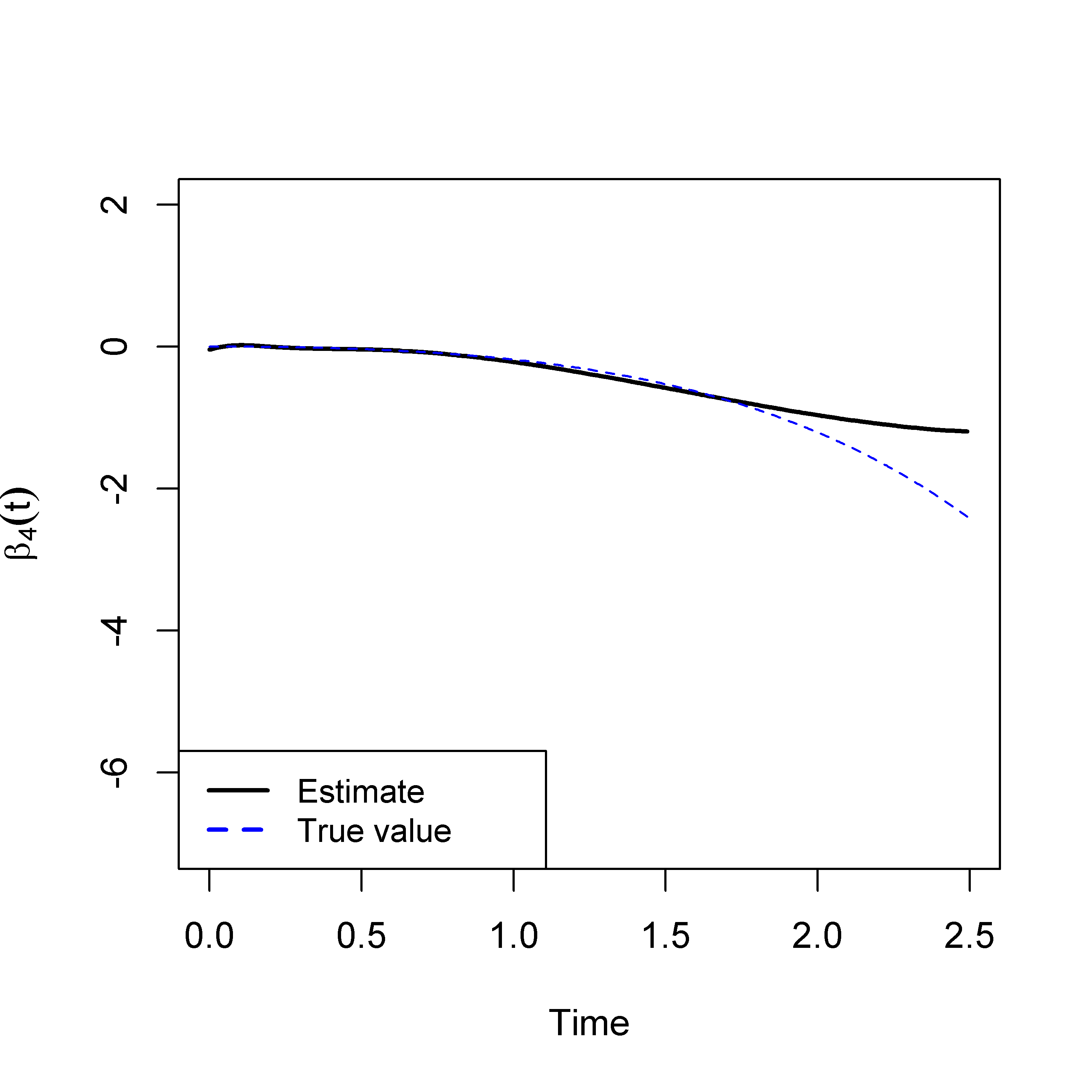
(l) Gradient: m=3,000

2.7 Numerical Properties

To derive the numerical properties for the MMSA, we impose the following regularity conditions:

1. For any initial value $\boldsymbol{\theta}^{(0)}$, the block diagonal matrix, $\mathbf{H}(\boldsymbol{\theta})$, is positive definite in the super-level set $\{\boldsymbol{\theta}:\ell(\boldsymbol{\theta})\geq\ell(\boldsymbol{\theta}^{(0)})\}.$

2. The negative log-partial likelihood function is coercive; i.e., $\lim_{||\boldsymbol{\theta}||_{2}\rightarrow\infty}-\ell(\boldsymbol{\theta})=\infty.$

Condition (A) guarantees the existence of the MMSA update and is satisfied in most practical applications. The coercive assumption [26] defined in Condition (B) and the fact that the log-partial likelihood is upper bounded guarantee that the super-level set is compact. Therefore, the maximum value of $\ell(\boldsymbol{\theta})$ is attained, e.g. Weierstrasss’s theorem [26]. The existence of a cluster point of the MMSA is also guaranteed by the compactness.

We now show that there exists a learning rate $\nu$ such that the proposed algorithm satisfies the ascent property, which guarantees that the iterative estimates in each MMSA step serve as refinements of the previous step. Let $\lambda_{max}(\cdot)$ represent the largest eigenvalues of an arbitrary non-negative definite matrix. At each MMSA iteration, given the current estimates $\boldsymbol{\widehat{\theta}}^{(m-1)}$, let $\boldsymbol{\widetilde{\theta}}$ be a vector that lies between $\boldsymbol{\theta}$ and $\boldsymbol{\widehat{\theta}}^{(m-1)}$ such that

$$\ell(\boldsymbol{\theta})=\ell(\widehat{\boldsymbol{\theta}}^{(m-1)})+\triangledown\ell(\widehat{\boldsymbol{\theta}}^{(m-1)})^{T}(\boldsymbol{\theta}-\widehat{\boldsymbol{\theta}}^{(m-1)})+\frac{1}{2}(\boldsymbol{\theta}-\widehat{\boldsymbol{\theta}}^{(m-1)})^{T}\triangledown^{2}\ell(\boldsymbol{\widetilde{\theta}})(\boldsymbol{\theta}-\widehat{\boldsymbol{\theta}}^{(m-1)}).$$

Proposition 1 (Ascent Property) Assume Condition (A) holds. For $\nu>0$ satisfying

$$\lambda_{max}\left(\{\mathbf{H}(\boldsymbol{\widehat{\theta}}^{(m-1)})\}^{-1/2}\{-\triangledown^{2}\ell(\boldsymbol{\widetilde{\theta}})\}\{\mathbf{H}(\boldsymbol{\widehat{\theta}}^{(m-1)})\}^{-1/2}\right)<1/\nu,$$ (7)

we have

$$g(\boldsymbol{\theta}|\widehat{\boldsymbol{\theta}}^{(m-1)})\leq\ell(\boldsymbol{\theta})~{}~{}\mbox{for all}~{}~{}\boldsymbol{\theta}.$$

Proposition 1 shows that $g(\boldsymbol{\theta}|\widehat{\boldsymbol{\theta}}^{(m-1)})$ serves as a minority surrogate function of $\ell(\boldsymbol{\theta})$. Thus, the resulting estimates $\widehat{\boldsymbol{\theta}}^{(m)}$ from the MMSA ensure the ascent property

$$\ell(\widehat{\boldsymbol{\theta}}^{(m)})\geq g(\widehat{\boldsymbol{\theta}}^{(m)}|\widehat{\boldsymbol{\theta}}^{(m-1)})\geq g(\widehat{\boldsymbol{\theta}}^{(m-1)}|\widehat{\boldsymbol{\theta}}^{(m-1)})=\ell(\widehat{\boldsymbol{\theta}}^{(m-1)}),$$

and serve as refinements of the previous step.

Proposition 1 also helps clarify when a small learning rate is needed and provides insights into the choice of norm for (2) in practical implementations. For example, for classical gradient-based procedures, the updates at each iteration are computed based on gradient information only. To ensure the ascent property for such gradient-based algorithms, the learning rate $\nu$ is required to satisfy $\lambda_{max}\left(\{-\triangledown^{2}\ell(\boldsymbol{\widetilde{\theta}})\}\right)<1/\nu.$ This may explain the previous finding that the learning rate $\nu$ is typically chosen to be sufficiently small for classical gradient boosting to ensure better predictive and estimation accuracy. However, a small value of $\nu$ requires a large number of boosting iterations and thus more computing time, especially when the condition numbers of the observed information matrix are large as exemplified in the estimation of time-varying effects. In contrast, the proposed MMSA is less sensitive to the choice of learning rate and substantially improves the computational efficiency. As shown in Figure 3, compared with gradient-based procedure, the proposed method achieves much computational efficiency and more accurate updates.

Proposition 2 (Numerical Convergence) Assume the same condition on the learning rate as in Proposition 1. Suppose Conditions (A) and (B) hold. Then every cluster point of the iterates $\boldsymbol{\widehat{\theta}}^{(m)}=M(\boldsymbol{\widehat{\theta}}^{(m-1)})$ generated by the iteration map $M(\boldsymbol{\theta})$ of the MMSA algorithm is a stationary point of $\ell(\boldsymbol{\theta})$. Furthermore, the set of stationary points $\mathcal{F}$ is closed and the limit of the distance function is zero:

$$\lim_{m\rightarrow\infty}\inf_{\boldsymbol{\theta}\in\mathcal{F}}||\boldsymbol{\widehat{\theta}}^{(m)}-\boldsymbol{\theta}||_{2}=0.$$

Moreover, if the observed information matrix $-\triangledown^{2}\ell(\boldsymbol{\theta})$ is positive definite in the super-level set defined in Condition (A), any sequence of $\boldsymbol{\widehat{\theta}}^{(m)}$ possesses a limit, and this limit is a stationary point of $\ell(\boldsymbol{\theta})$.

2.8 Testing for Time-Varying Effects

To assign p-values to determine whether the covariate effects are time-varying, we explore the following property of B-splines: if $\theta_{p1}=\cdots=\theta_{pK}=\theta,$ the corresponding covariate effect is time-independent; e.g.,

$$\beta_{p}(t)=\sum_{k=1}^{K}\theta_{pk}B_{k}(t)=\theta.$$

Specify a matrix $\mathbf{C}_{p}$ such that $\mathbf{C}_{p}\boldsymbol{\theta}=\textbf{0}$ corresponds to the contrast that $\theta_{p1}=\cdots=\theta_{pK}$. A Wald test can then be constructed by

$$(\mathbf{C}_{p}\boldsymbol{\widehat{\theta}})^{T}(\mathbf{C}_{p}(-\triangledown^{2}\ell(\boldsymbol{\widehat{\theta}}))^{-1}\mathbf{C}_{p}^{T})^{-1}(\mathbf{C}_{p}\boldsymbol{\widehat{\theta}}),$$

where $\boldsymbol{\widehat{\theta}}$ is obtained through the proposed MMSA.

In the kidney transplant database, however, computation of the observed information matrix outpowers a computer with an 32G memory. Numerically, the gradients are much easier to compute. Therefore, we consider the following test

$$S_{p}=(\mathbf{C}_{p}\boldsymbol{\widehat{\theta}})^{T}(\mathbf{C}_{p}\mathbf{V}^{-1}(\boldsymbol{\widehat{\theta}})\mathbf{C}_{p}^{T})^{-1}(\mathbf{C}_{p}\boldsymbol{\widehat{\theta}}),$$

where

$$\mathbf{V}(\boldsymbol{\widehat{\theta}})=\sum_{j=1}^{J}\sum_{i=1}^{n_{j}}\Psi_{ij}(\boldsymbol{\widehat{\theta}})\Psi_{ij}(\boldsymbol{\widehat{\theta}})^{T}$$

is an approximation of the empirical information matrix, with

$$\Psi_{ij}(\boldsymbol{\widehat{\theta}})=\delta_{ij}\left\{\mathbf{X}_{ij}-\overline{\textbf{Z}}_{ij}(\widehat{\boldsymbol{\theta}},T_{ij})\right\}\otimes\textbf{B}(T_{ij}).$$

Here $\otimes$ is the Kronecker product and

$$\overline{\textbf{Z}}_{ij}(\widehat{\boldsymbol{\theta}},T_{ij})=\frac{\sum_{i^{\prime}\in R_{ij}}\textbf{X}_{i^{\prime}j}\exp\{\textbf{X}_{i^{\prime}j}^{T}\widehat{\boldsymbol{\Theta}}\textbf{B}(T_{ij})\}}{\sum_{i^{\prime}\in R_{ij}}\exp\{\textbf{X}_{i^{\prime}j}^{T}\widehat{\boldsymbol{\Theta}}\textbf{B}(T_{ij})\}}.$$

Under the null hypothesis that the covariate effect is time-independent, the statistics $S_{p}$ is asymptotically chi-square distributed with $K-1$ degree of freedom.

3 Simulations

We consider the following simulation settings:

• Death times were generated from an exponential model with a baseline hazard 0.5. Censoring times were generated from the Uniform (0,3) distribution. Continuous predictors were generated from a multivariate normal distribution, where the covariance followed an AR1 with an auto-correlation parameter 0.6. We varied the number of predictors from 5, 20 to 50. We chose $\beta_{2}(t)=sin3(\pi t/4)$ and $\beta_{4}(t)=-(t/3)^{2}\exp(t/2)$ to represent time-varying effects. The remaining covariate effects were set as constants (e.g. time-independent effects).

• To mimic the motivating real data example, binary covariates were generated with specified frequencies between 0.05 and 0.2. The remaining simulation set-ups were the same as Setting 1.

• Two continuous covariates were generated with coefficients $\beta_{1}=1$ and $\beta_{2}(t)=\gamma\cdot\mbox{sin}(3(\pi t/4))$, where $\gamma$ varied between 0 and 3, representing the magnitude of the time-varying effects. The remaining simulation set-ups were the same as Setting 1.

3.1 Evaluation of Computation Speed

Table 1 compares the computation time for the proposed MMSA and the Kronecker product-based Newton method (implemented in Rcpp through R package RcppArmadillo) with step size determined by backtracking line search [1], quasi-Newton method (He et al. [20]; implemented by R function optim), and the likelihood-based boosting (termed as L-Boost and implemented by R package COX_flexBoost). The simulation set-up was based on Setting 1 with various combinations of sample sizes and numbers of predictors. The convergence criterion was chosen as the maximal absolute change of $\boldsymbol{\theta}$ or the change of $\ell(\boldsymbol{\theta})$ less than $10^{-6}$. These timings were taken on a HP workstation with 4-core 3.50-GHz Intel Core E5-1620v3 processor and 32GB RAM. When the sample size is very large, no results are reported for the competing methods due to the computation exceeding the computer’s maximum memory capacity.

Table 1: Computation Time: n=sample size; J=number of centers; P=number of covariates; NA for L-Boost: no results are reported due to its intensive computation; NA for Newton or quasi-Newton: the computation exceeds the computer’s max memory capacity; based on Setting 1.

n	J	P	Newton	quasi-Newton	L-Boost	MMSA
1,000	1	10	0.08 minutes	15.43 minutes	10.36 hours	0.34 minutes
10,000	10	20	1.12 minutes	1.93 hours	NA	7.15 minutes
347,668	293	164	NA	NA	NA	11.64 hours

Figure 4: Estimated coefficients (solid lines) and 95% confidence interval (dashed lines) for simulation setting 1; $n=1,000$, $p=10$; $\beta_{2}(t)=sin3(\pi t/4)$ and $\beta_{4}(t)=-(t/3)^{2}\exp(t/2)$ are time-varying effects; $\beta_{1}=1$ and $\beta_{3}=-1$ are constant effects; K: number of B-spline basis functions; based on Setting 1.

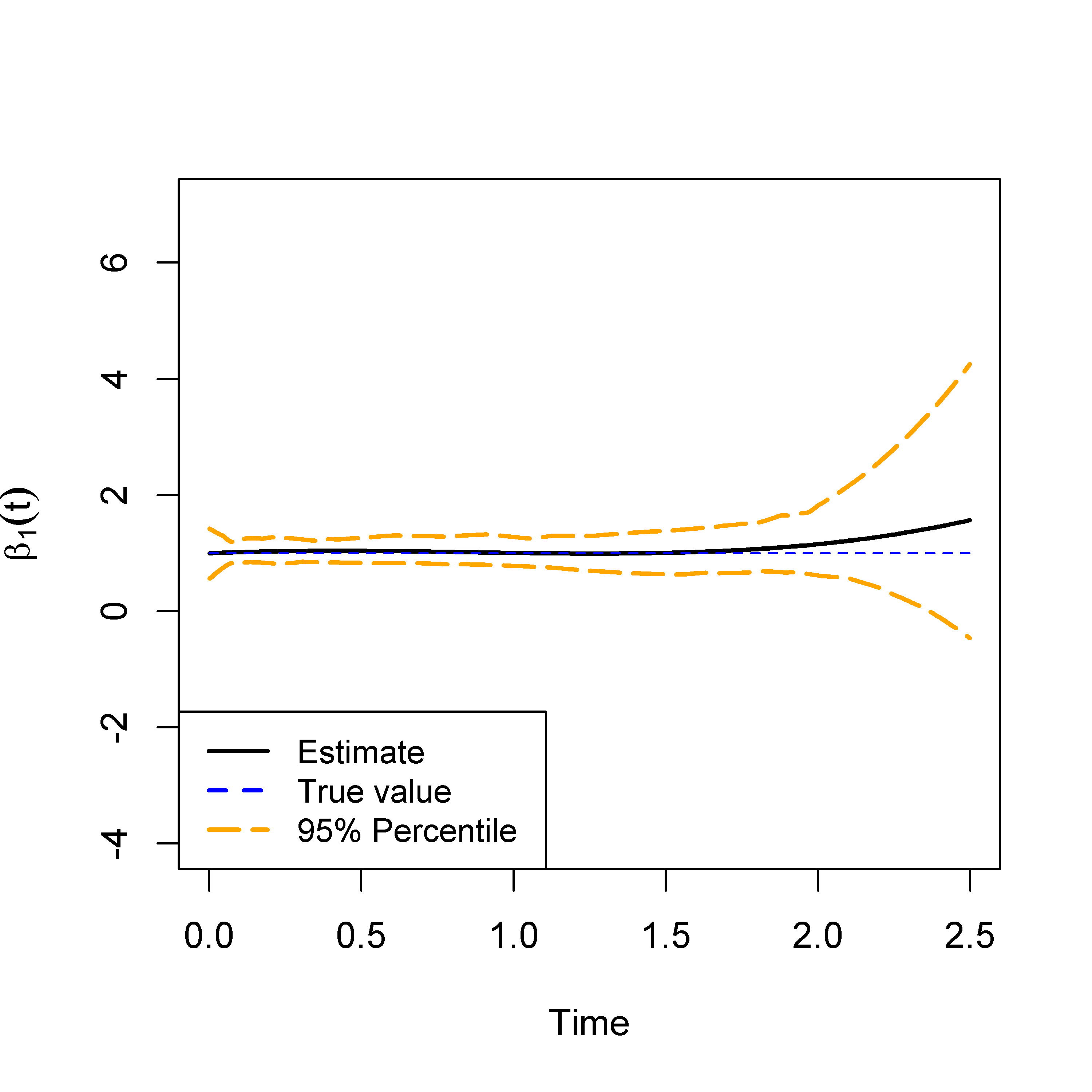
(a) Newton (K=5)

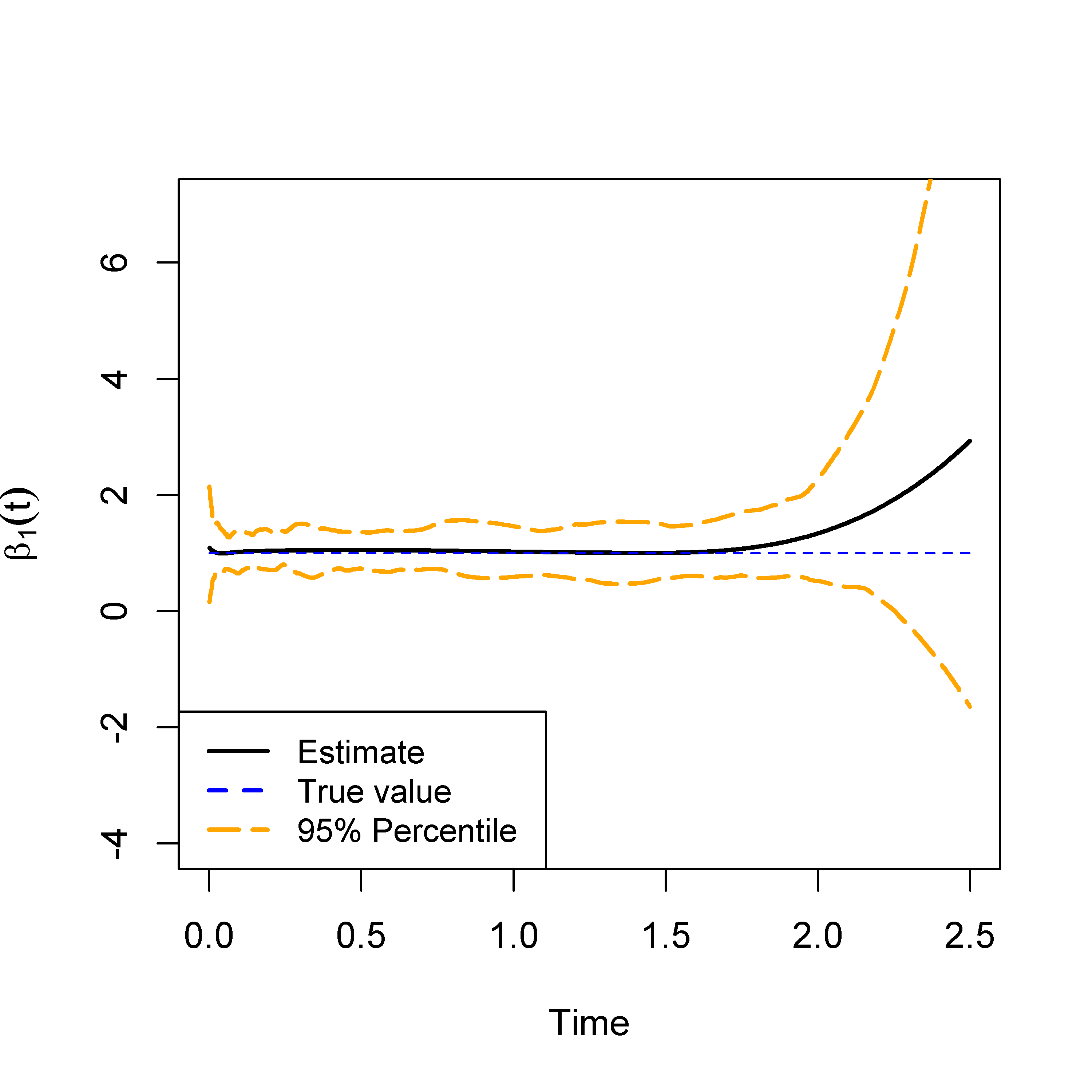
(b) Newton (K=10)

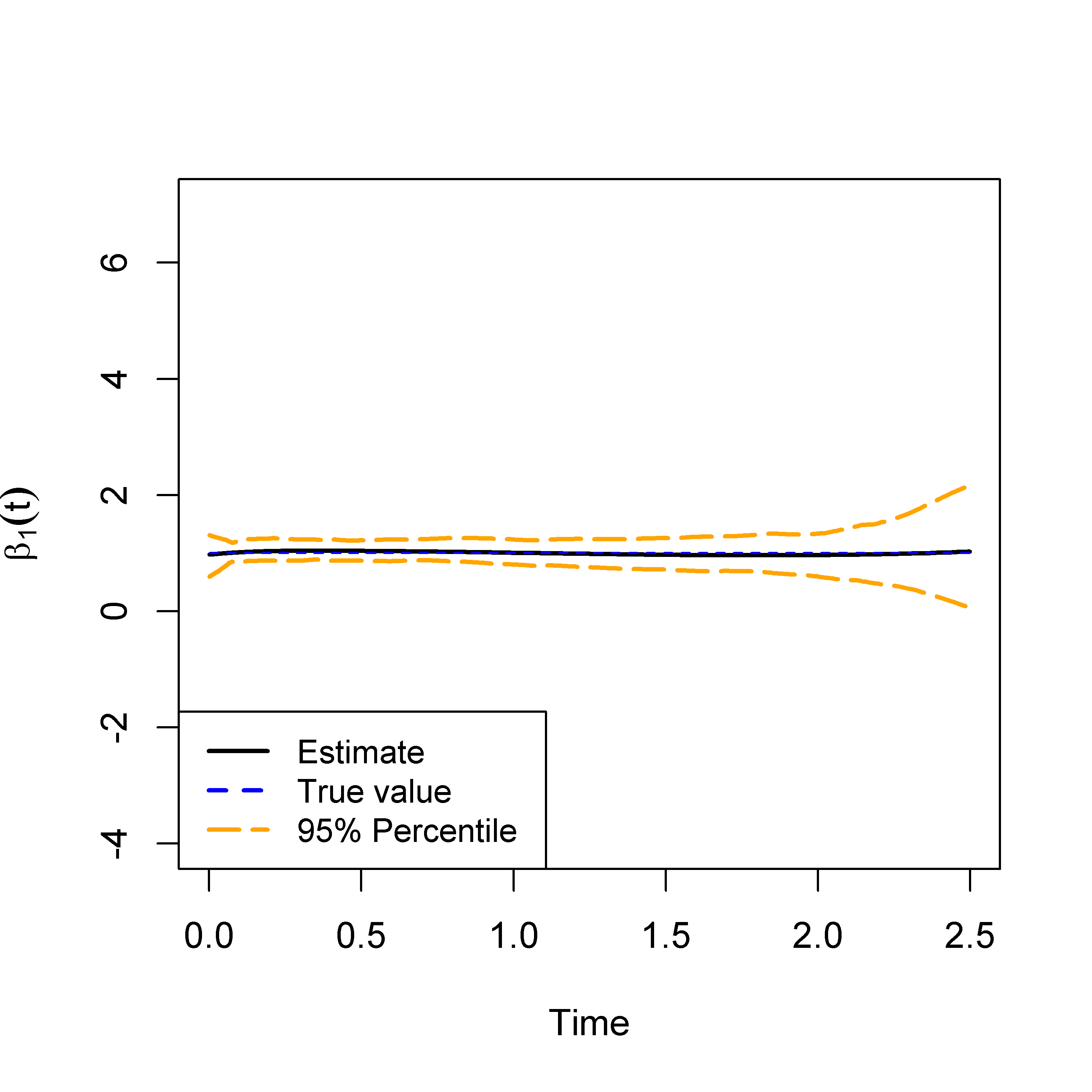
(c) MMSA (K=5)

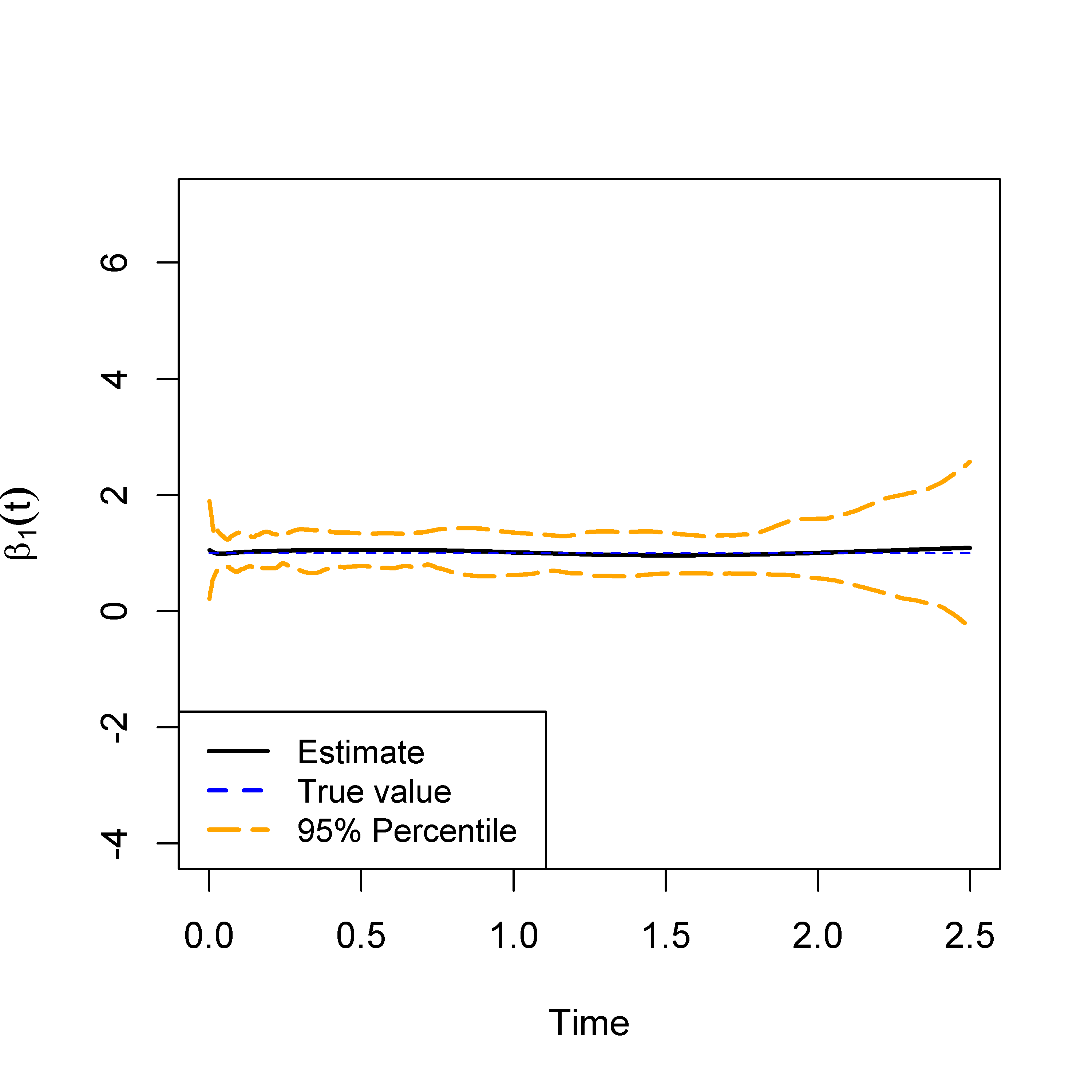
(d) MMSA (K=10)

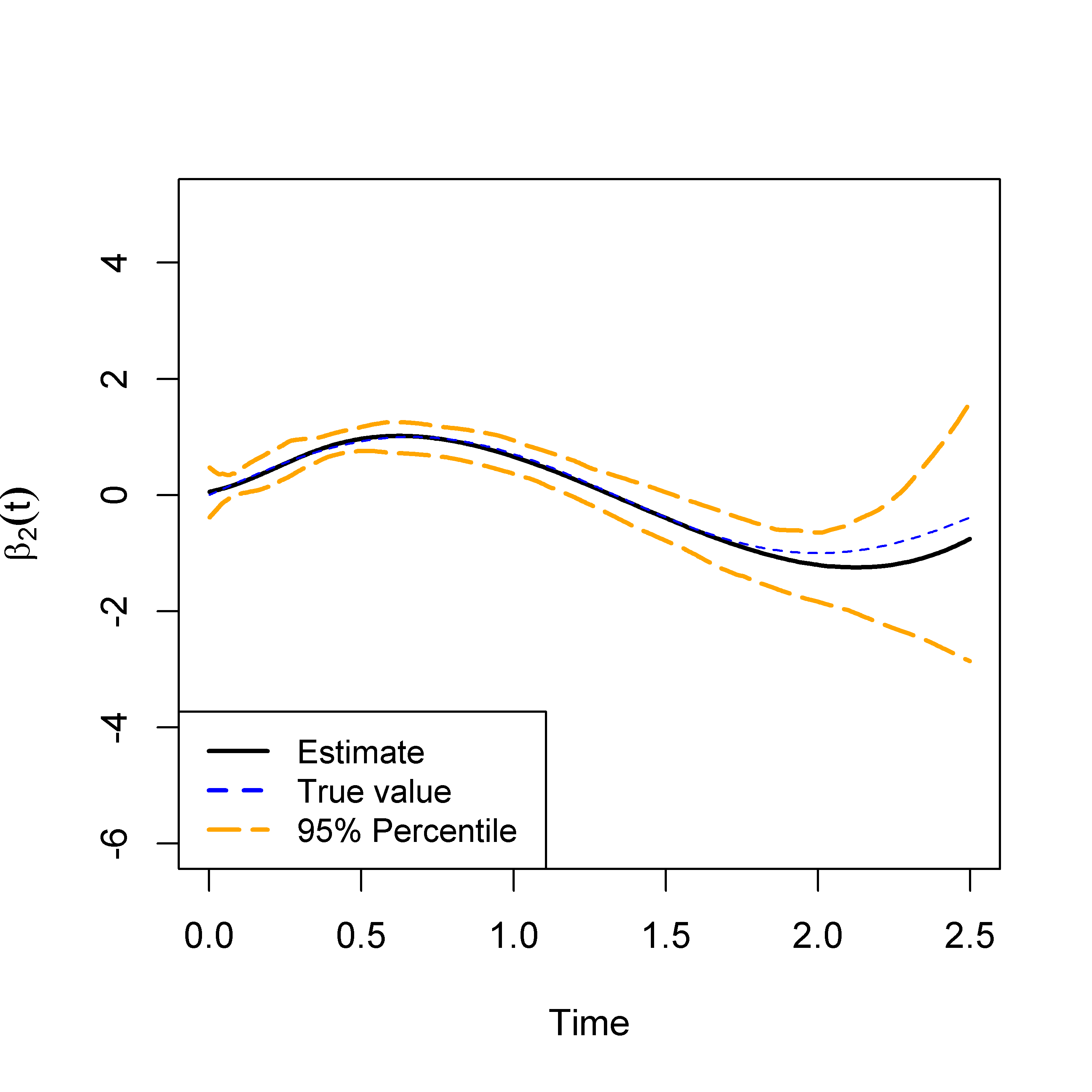
(e) Newton (K=5)

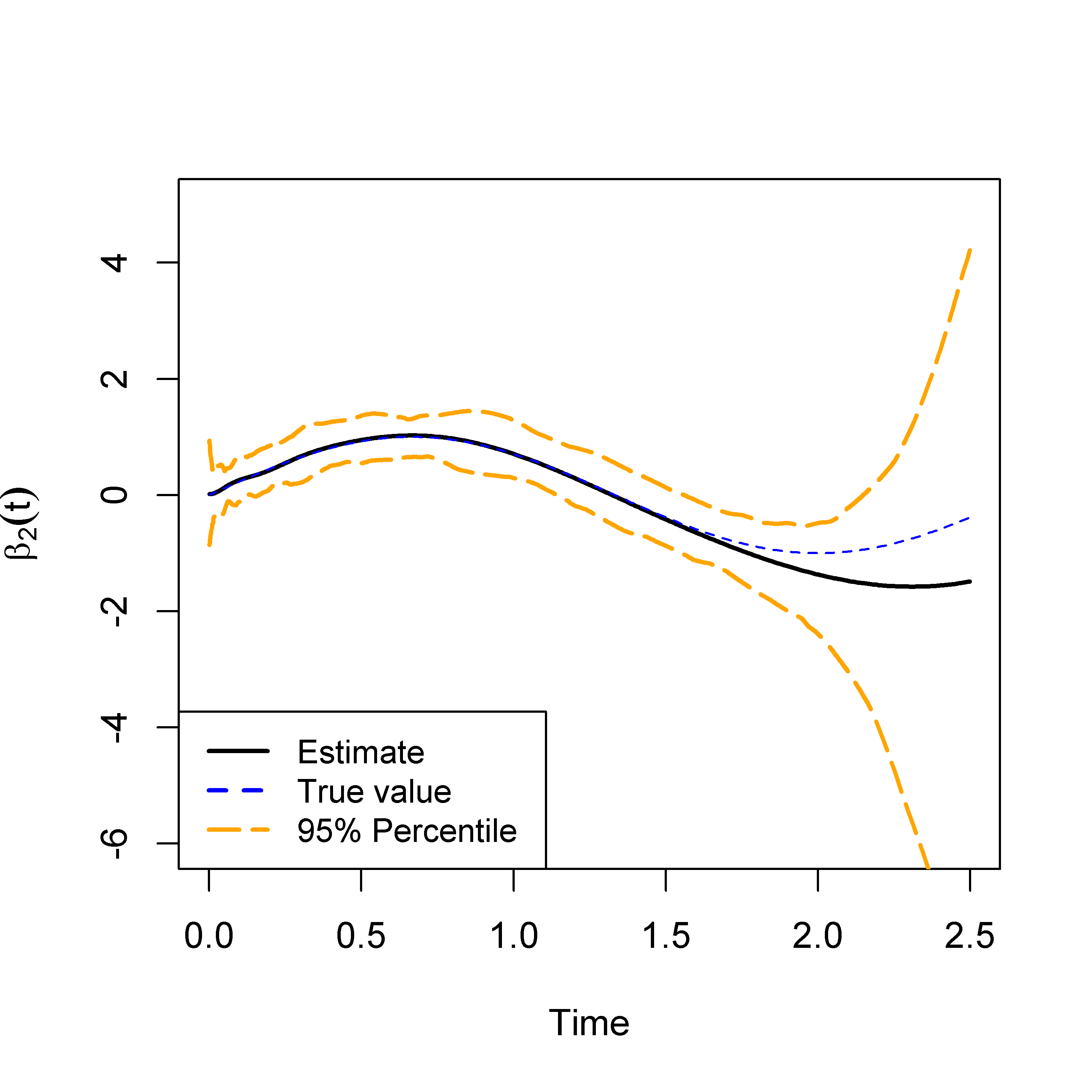
(f) Newton (K=10)

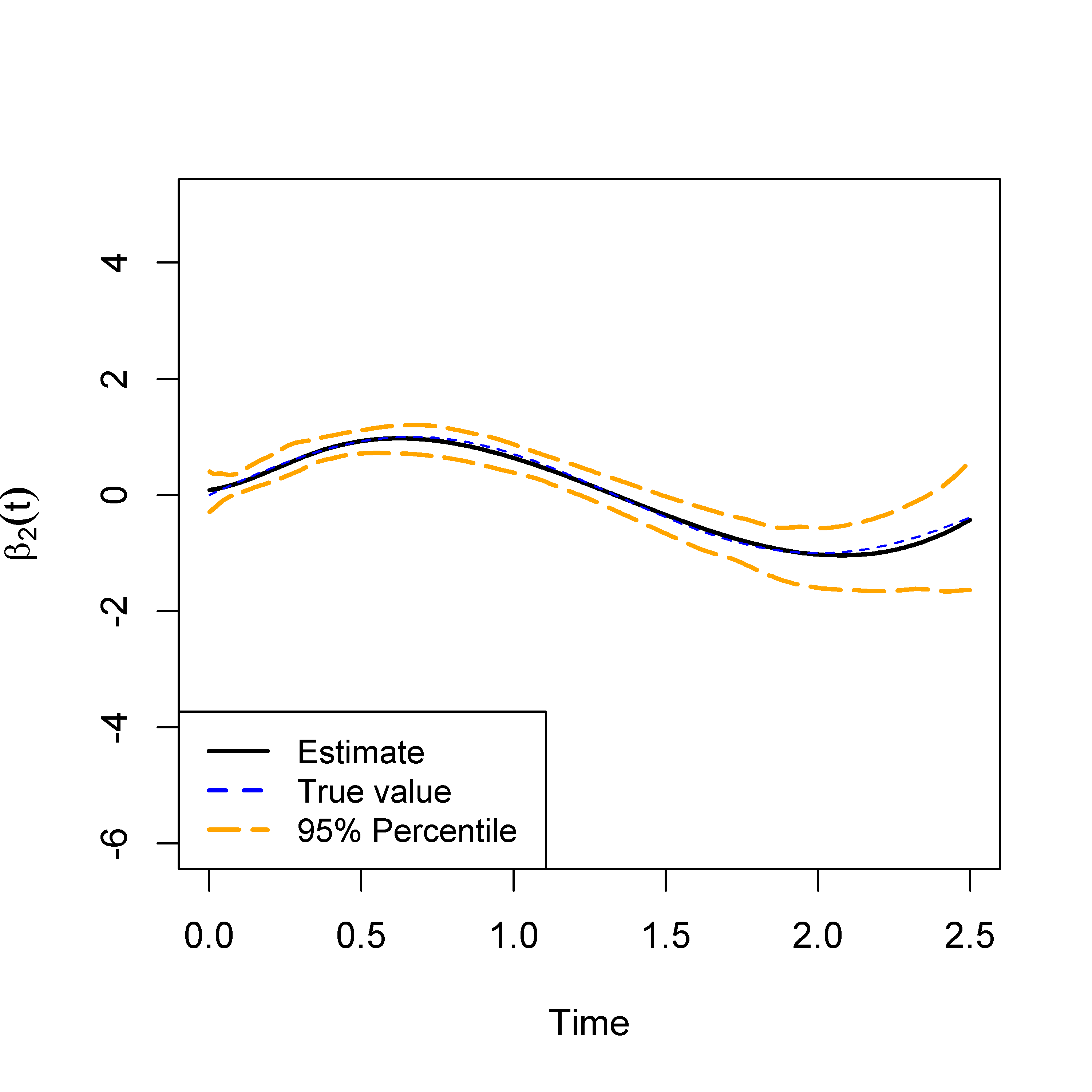
(g) MMSA (K=5)

(h) MMSA (K=10)

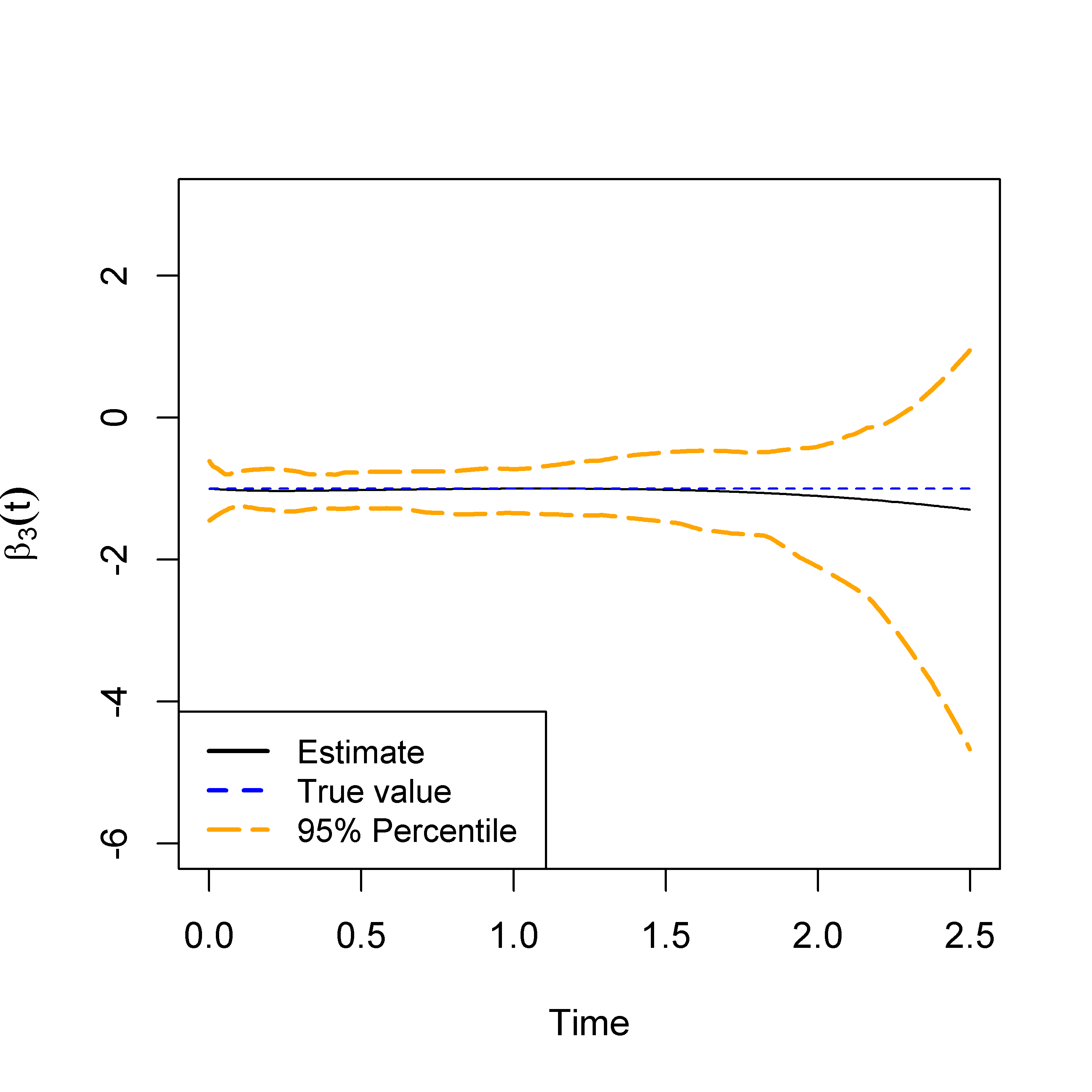
(i) Newton (K=5)

(j) Newton (K=10)

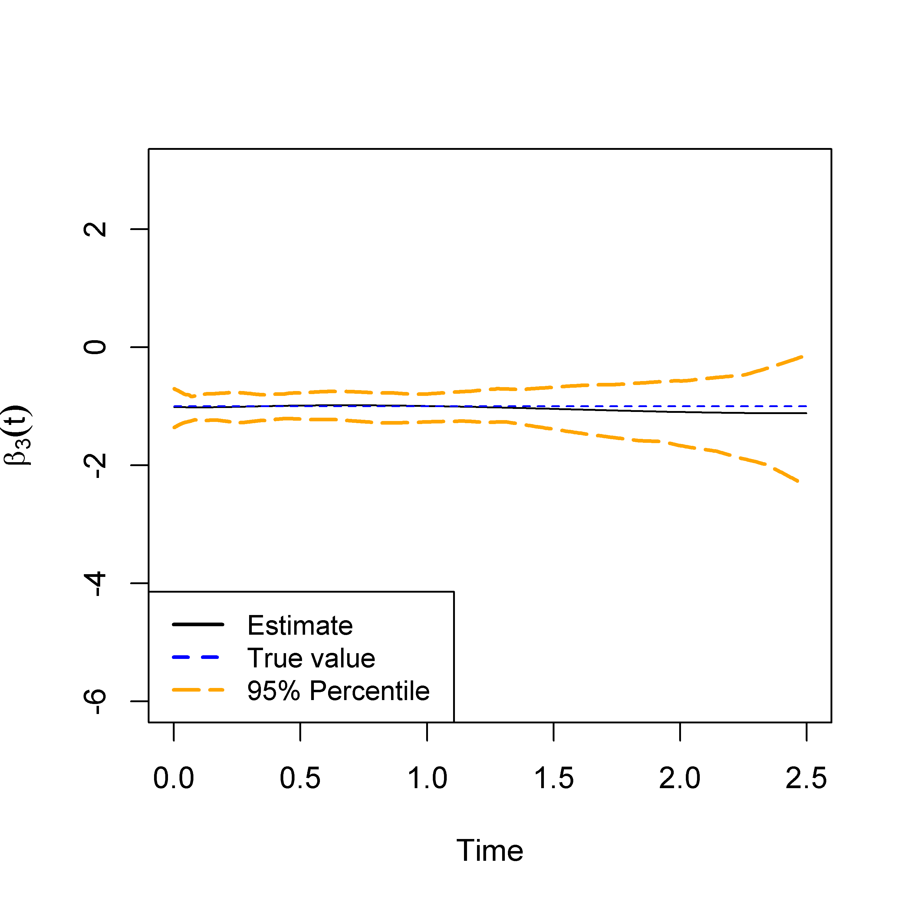
(k) MMSA (K=5)

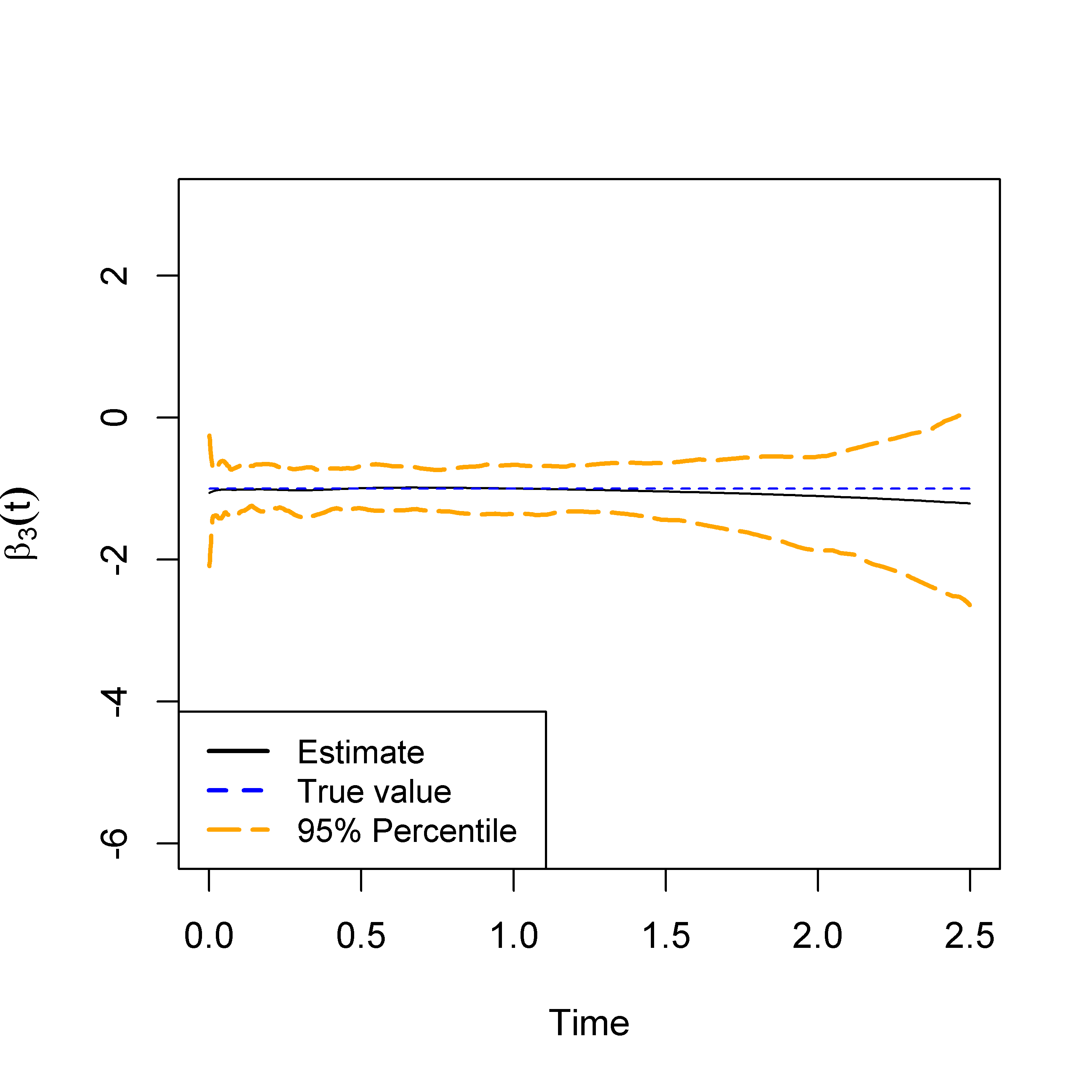
(l) MMSA (K=10)

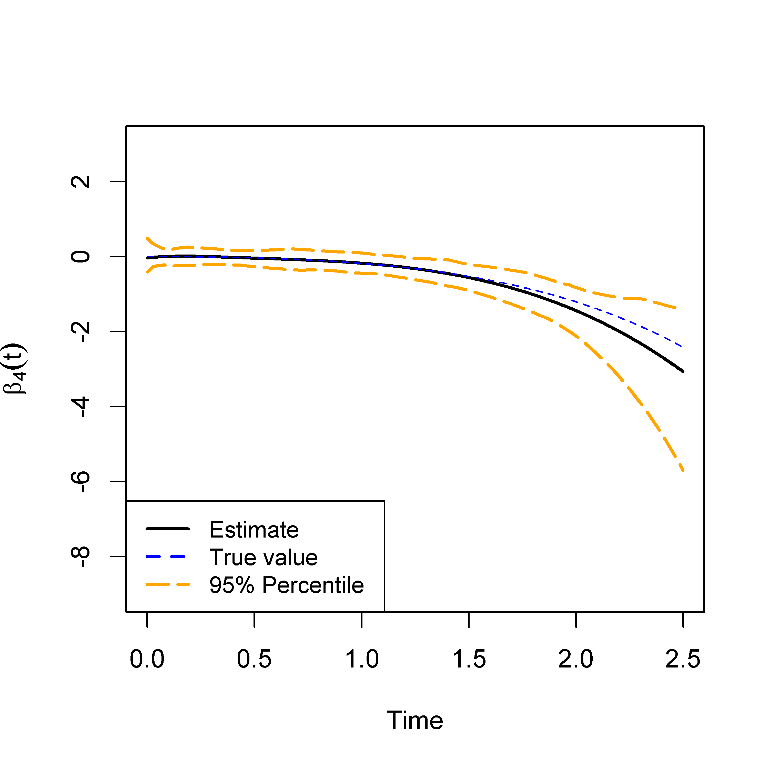
(m) Newton (K=5)

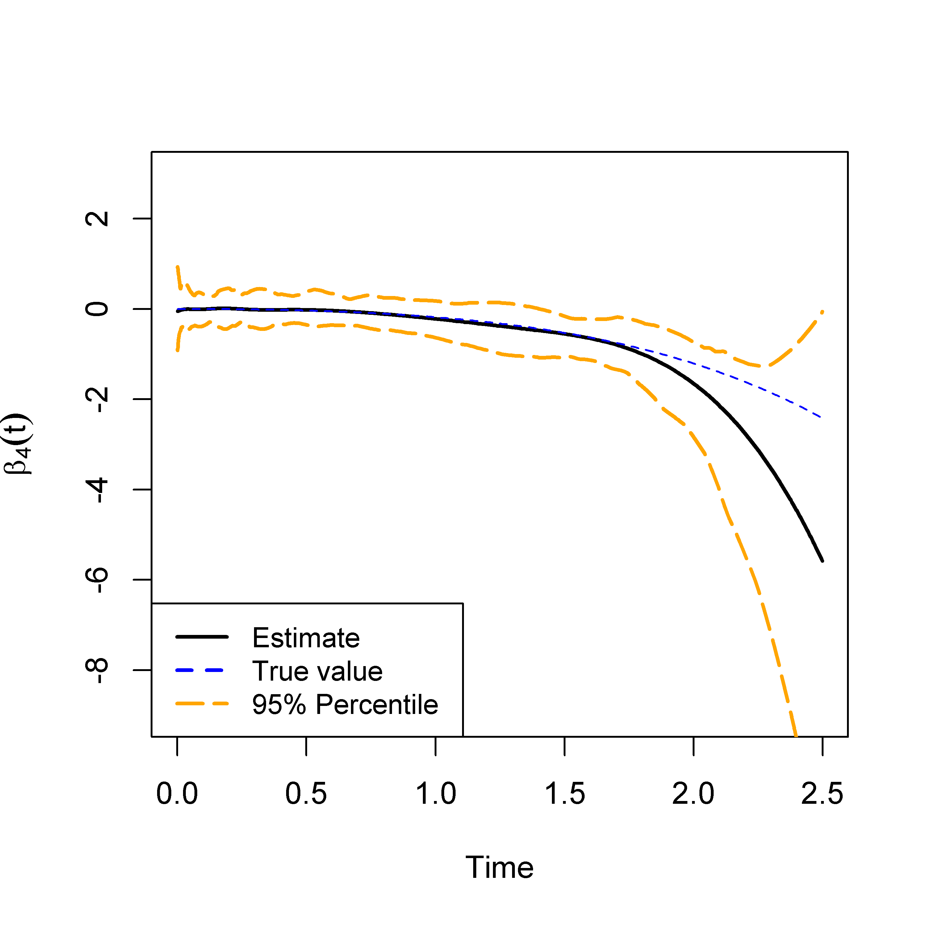
(n) Newton (K=10)

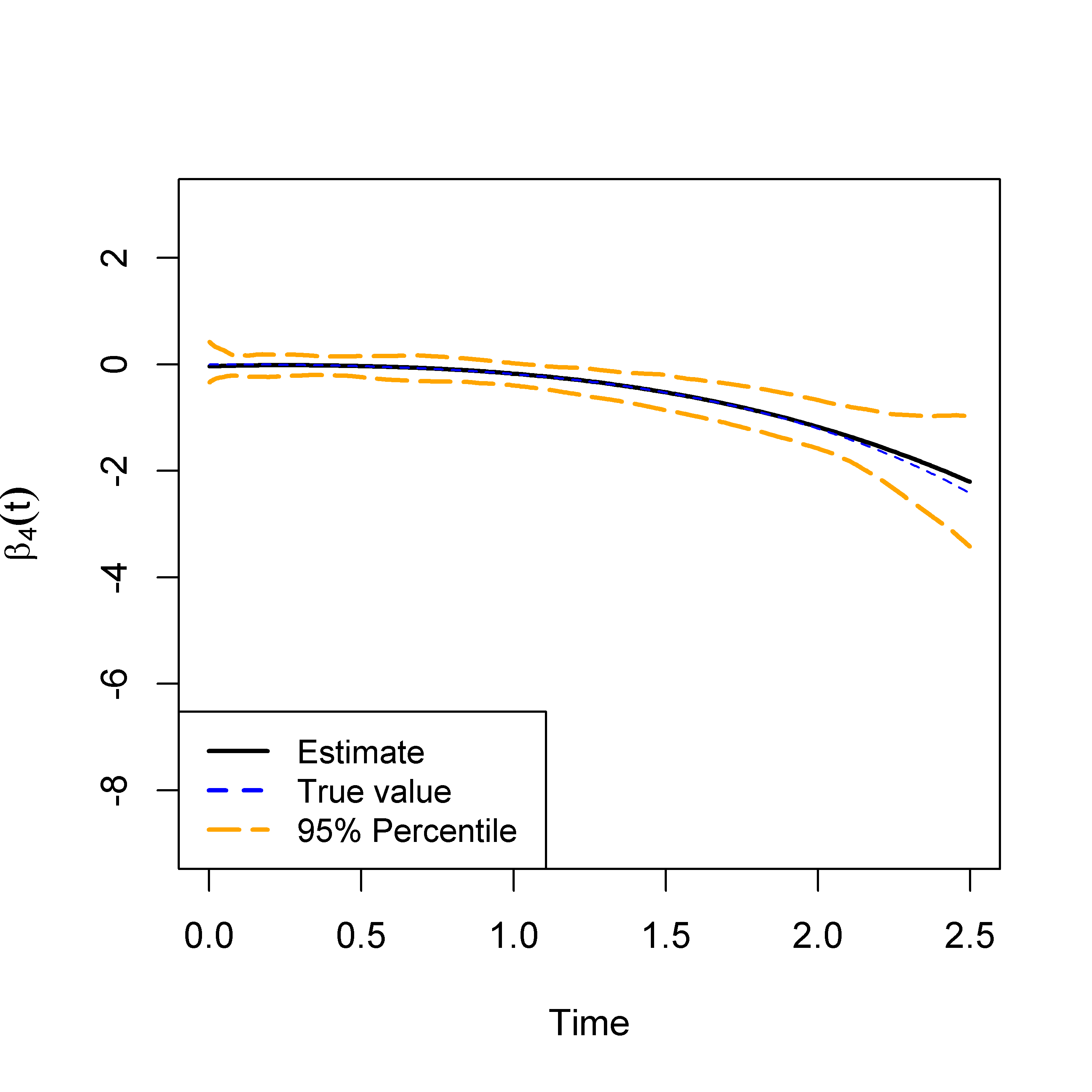
(o) MMSA (K=5)

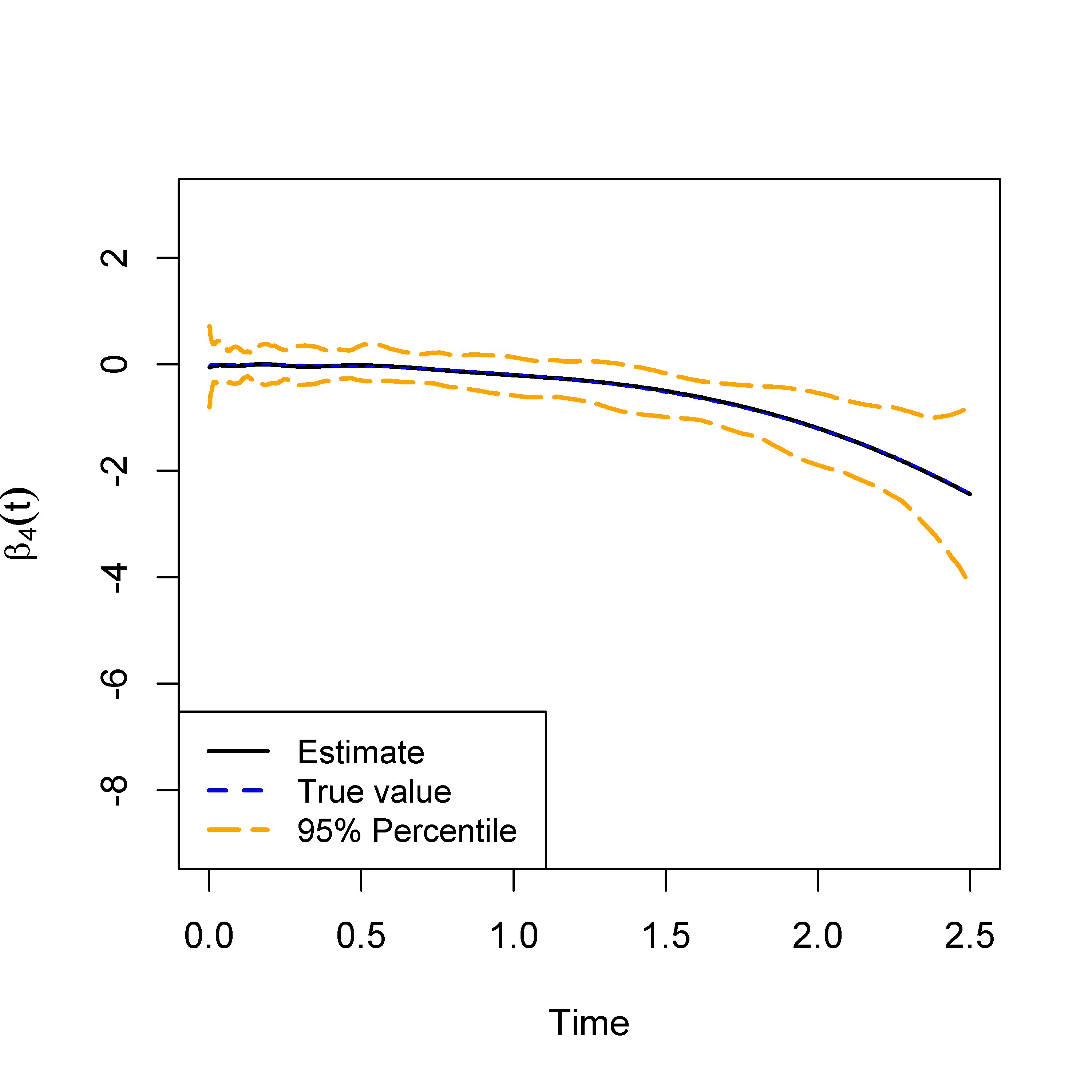
(p) MMSA (K=10)

3.2 Estimation of Time-Varying Effects

Table 2: Average computation time (in seconds), average estimation error (Bias) and average integrated mean square error (IMSE) for various methods; based on Setting 2.

P		Method	Time	Bias	IMSE
5		Newton	0.22	0.646	0.592
		Coordinate Ascent	356.09	0.810	0.632
		Gradient Ascent	169.33	0.249	0.202
		Stochastic Gradient Ascent	183.51	0.290	0.256
		MMSA	25.60	0.156	0.136
20		Newton	1.10	0.305	0.169
		Coordinate Ascent	1260.24	0.184	0.186
		Gradient Ascent	687.15	0.136	0.058
		Stochastic Gradient Ascent	415.43	0.140	0.070
		MMSA	43.48	0.075	0.055
50		Newton	9.05	0.147	0.086
		Coordinate Ascent	2760.26	0.807	0.224
		Gradient Ascent	1620.21	0.150	0.050
		Stochastic Gradient Ascent	757.07	0.118	0.038
		MMSA	95.27	0.064	0.030

Table 2 compares the average computation time, average estimation errors and average integrated mean square error (IMSE) for the Newton approach, the coordinate ascent approach [8], the gradient ascent, and the stochastic gradient ascent with step size determined by Adagrad algorithm [35]. The reported bias and IMSE were the averages of point-wise estimates over simulated time points. The simulation set-up was based on Setting 2 with sample size 10,000 and various numbers of predictors. For each configuration, a total of 100 independent data were generated. As shown in Table 2, the Newton and coordinate ascent approaches suffer from large estimation biases and IMSE. The gradient ascent, and the stochastic gradient ascen substantially improve the estimation errors, but they suffer from slow convergence. In contrast, the proposed MMSA is computationally efficient and achieved the smallest estimation biases in all scenarios. Figure 3 further compares the average estimated coefficients across various iterations of the proposed method and the gradient ascent. Compared with gradient-based procedure, the proposed method achieves much computational efficiency and more accurate updates. Figure 4 compares the average estimates and the $95\%$ empirical percentiles over 100 simulation replications for the conventional Newton approach and the MMSA algorithm. We varied the number of basis functions from 5 to 10. The simulation set-up was based on Setting 1 with 10 variables. The poor performance of the Newton can be explained in part as follows: in the late stage of the follow-up period, the at-risk set is small, causing unstable estimation. In contrast, the proposed MMSA is less sensitive to the number of basis functions, achieving much more stable results.

3.3 Testing for Time-Varying Effects

We next compared the proposed testing algorithm and the test based on the scaled Schoenfeld residuals (implemented by R Survival package). Figures 5a and 5b compares the empirical Type-I error and the empirical power based on Setting 3. The proposed testing outperforms the traditional method with higher power to correctly identify the time-varying effects and smaller Type-I error for falsely identifying time-independent effects as time-varying (e.g. false positive). In contrast, the Type-I error for the test based on the scaled Schoenfeld residuals increased with the magnitude of the time-varying effect. One possible explanation is as follows: as noted in Grambsch and Therneau [14], the scaled Schoenfeld residuals are one-step Newton estimators with initial values fitted from the Cox proportional hazards model. When the magnitude of true time-varying effects is relatively large, the initial values are far away from the truth and hence, the one-step estimator may result in biased estimation.

Figure 5: Testing for time-varying effects at significance level 0.05; Type-I error: empirical probability of falsely identifying time-independent effects as time-varying; Power: empirical probabilities of correctly identifying the time-varying effects; based on Setting 3.

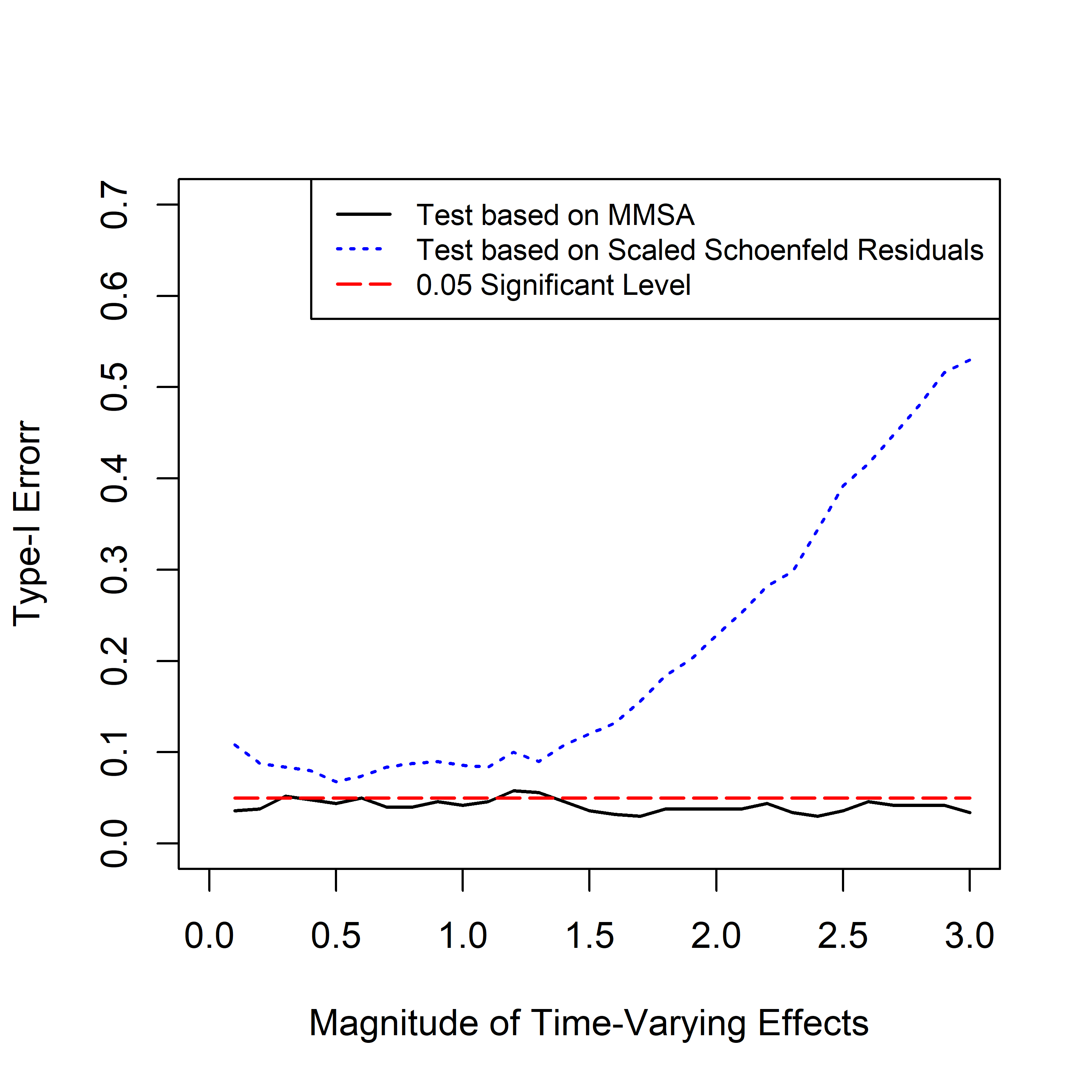
(a) Type I Error

(b) Power

4 Application

4.1 Kidney Transplant Dataset

Data were obtained from the U.S. Organ Procurement and Transplantation Network (OPTN). Included in our analysis were $347,668$ patients (from $293$ centers) who underwent kidney transplantation between January $1988$ and December $2012$. Patient survival was censored 10 year post-transplant or at the end of study (2012). Failure time (recorded in years) was defined as the time from transplantation to graft failure or death, whichever occurred first. The overall censoring rate was $62\%$. Adjustment covariates ($P=164$) in this study included baseline recipient characteristics such as age, race, gender, BMI, time on dialysis, indicator of previous kidney transplant, immunosuppression, and cormorbidity conditions (e.g. glomerulonephritis, polycystic kidney disease, diabetes, and hypertension), and donor characteristics such as blood type, cold ischemic time and type of donor kidney. Race was categorized as White, African American, Hispanic, Asian or other. Cold ischemia times were categorized as Low (20 hours or less) or High (longer than 20 hours). Type of donor kidney was categorized as living, standard criteria donor, or expanded criteria donor (ECD). Waiting times on dialysis were categorized as Short (less than 5 years) or Long (greater than 5 years).

4.2 Assessing Time-Varying Effects

To determine the number of basis functions, we performed 5-fold cross-validation [39]. Ten basis functions were chosen for further analysis. A total of 12 variables were identified with significant time-varying effects (p-values $<0.001$). Figures 6-7 show the fitted coefficients (solid lines) and 95% confidence intervals (dashed lines). Figures 6a and 6b show that anti-viral therapies and anti-rejection immunosuppressant medications had strong protective effects in the short term after transplantation, with a weakening association over time. One possible explanation is that these therapies prevent recipient’s body from rejecting new kidney and declining rates of acute rejection have led to improvements in short term kidney transplant survival [30]. Figure 6c strongly supports previous finding [29] that longer waiting times on dialysis (greater than 5 years) negatively impact post-transplant survival, especially in the short run. Figure 6d indicates that the effects of stroke, the most frequent donor cause of death, varies over time, showing an increased risk of worse recipient outcomes in the short run, and then a slightly weakening association over time. One possible explanation is as follows: although stroke is a predictor for worse survival for kidney transplantation, it is also associated with lower rates of rejection immediately after the renal transplantation [13], which may lead to varying association in the short run. Figure 6e suggests that the effect of Human leukocyte antigens (HLA) matching varies over time, resulting in an eventually weakening association. Thus, special care (such as pre-transplant antiviral therapy) must be dedicated to improve the long-term results. Figure 6f suggests that blood pressure management in the kidney transplant recipient reduces the likelihood of graft failure. Given the greater cardiovascular burden in the kidney transplant recipient, more effective control of blood pressure may further reduce cardiovascular-related death.

Figure 7a shows that male recipients is a protective factor immediately after the renal transplantation and then becomes a risk factor in the long run. Regarding racial disparities, Figure 7b indicates that survival outcomes for African Americans continue to lag behind non-African Americans. Our results for previous Kidney Transplant and high cold ischemic time (Figures 7c and 7d) show that they are risk factors for mortality in the short run. Thus, special care should be dedicated to improve the short-term results. As shown in Figure 7e, donors with higher height and hence larger adjusted cortical volume has a protective effect in the short-term after transplantation, which suggests that larger adjusted cortical volumes are more likely to achieve better glomerular filtration rate than those with smaller cortical volumes. Finally, polycystic kidney disease (PKD) is the most common genetic kidney disease, which accounts for 2% to 9% of patients with end-stage renal failure [34]. There are conflicting reports of differing renal allograft outcomes for PKD patients [17]. In our analysis, the time-varying coefficient (Figure 7f) suggests that there is a varying association of PKD. Thus, accounting for time-varying effects provides valuable clinical information that could be missed otherwise.

Figure 6: Transplant data: estimated coefficients (solid lines) and 95% confidence interval (dashed lines) for time-varying effects.

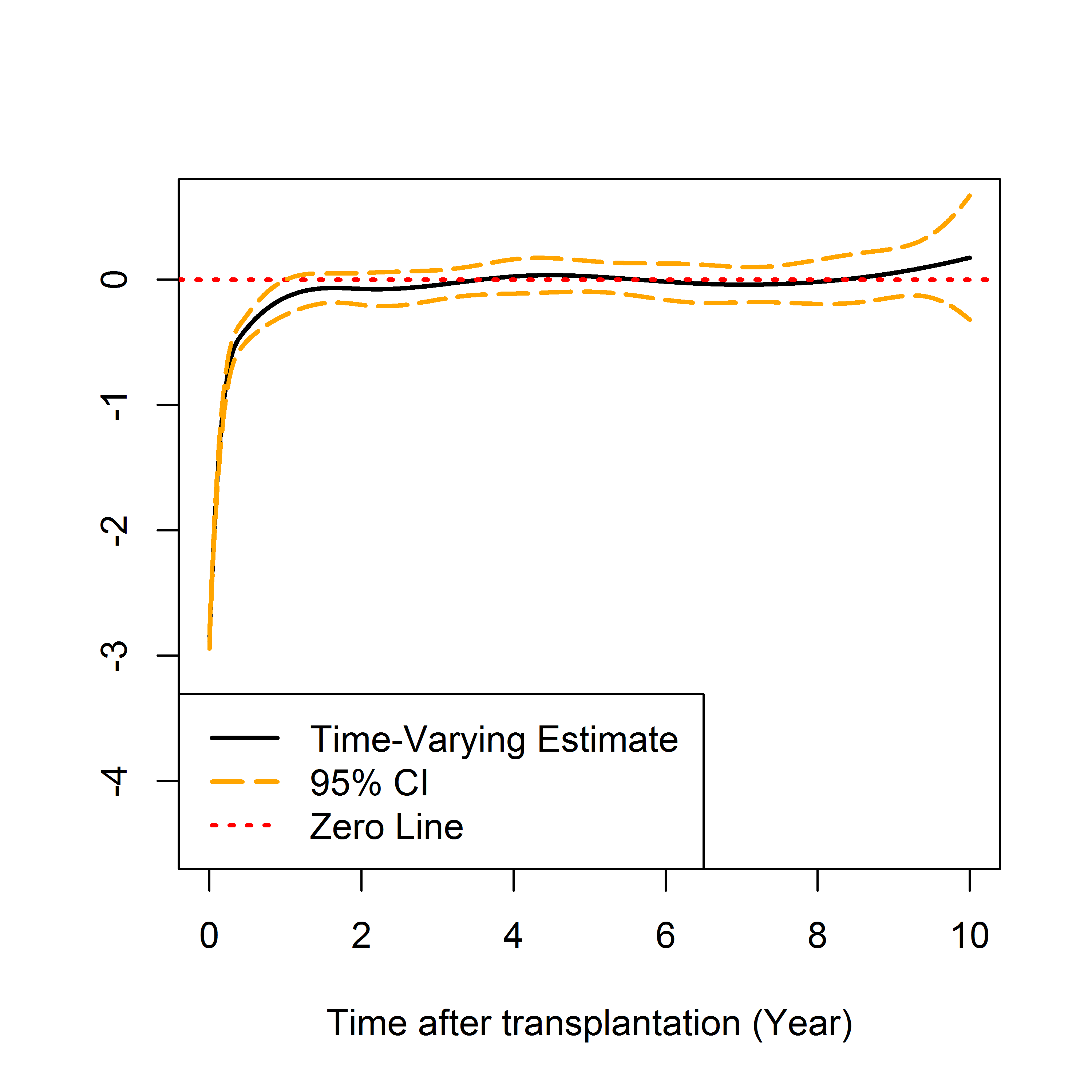
(a) Anti-viral Therapies

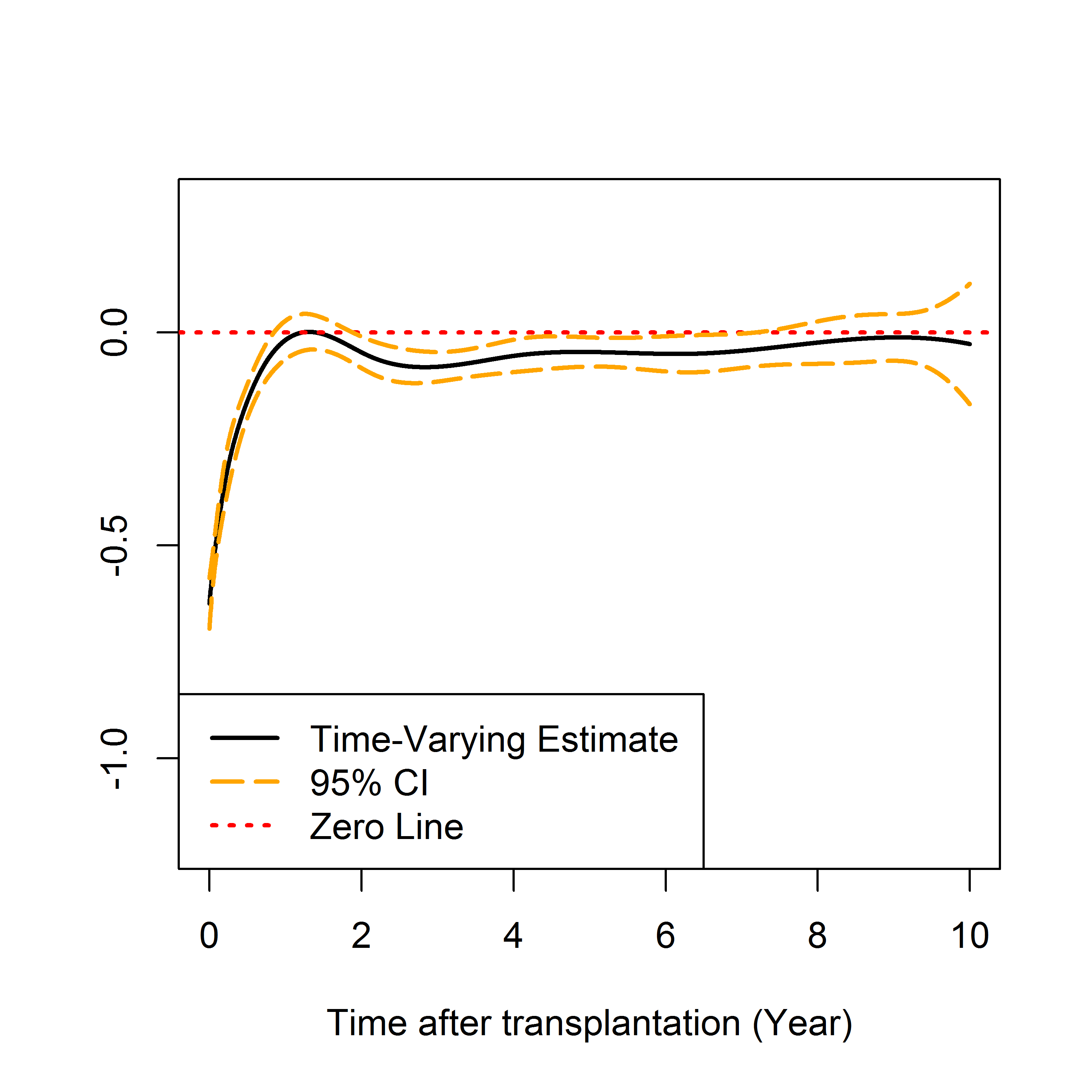
(b) Immunosuppressant Medications

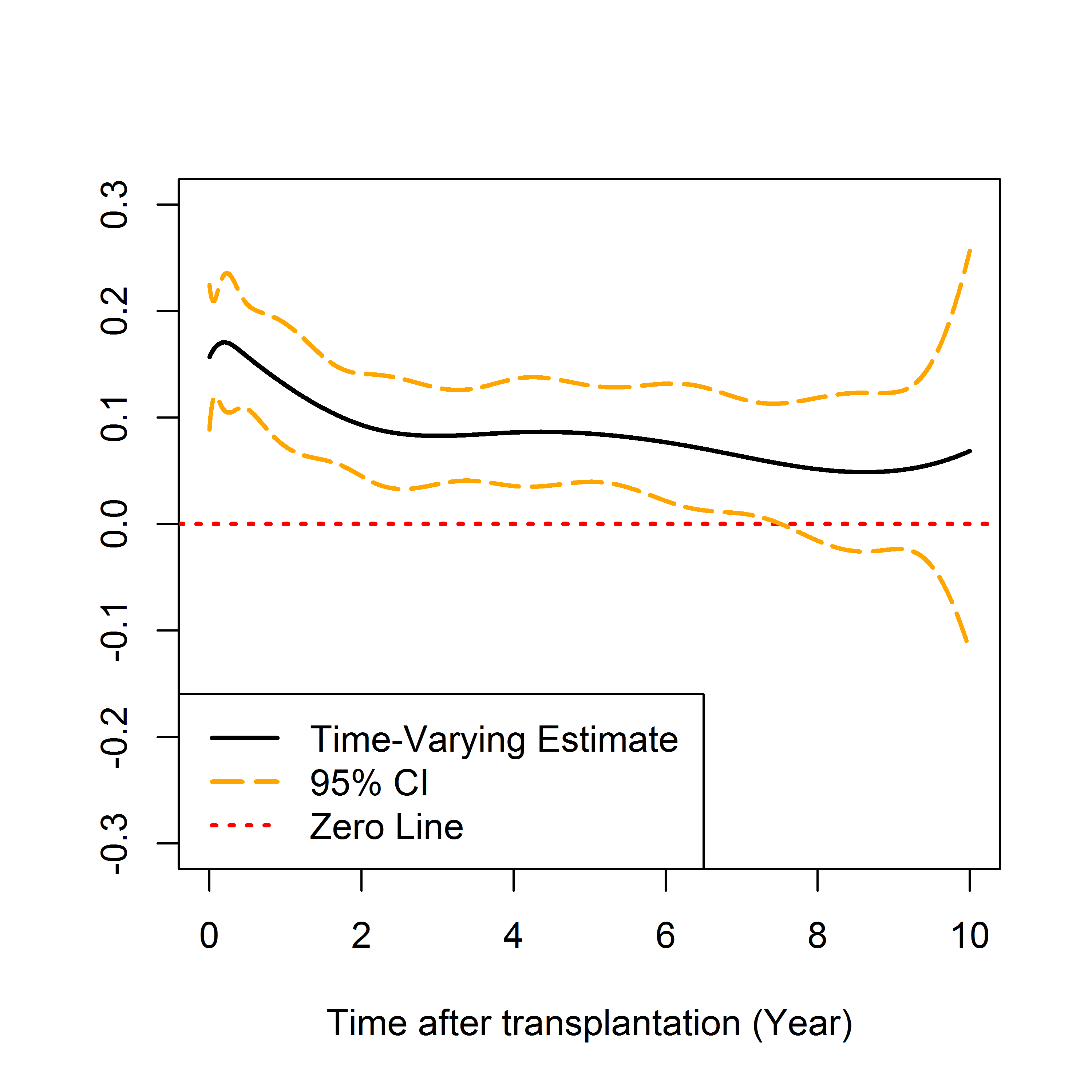
(c) Long Waiting Times

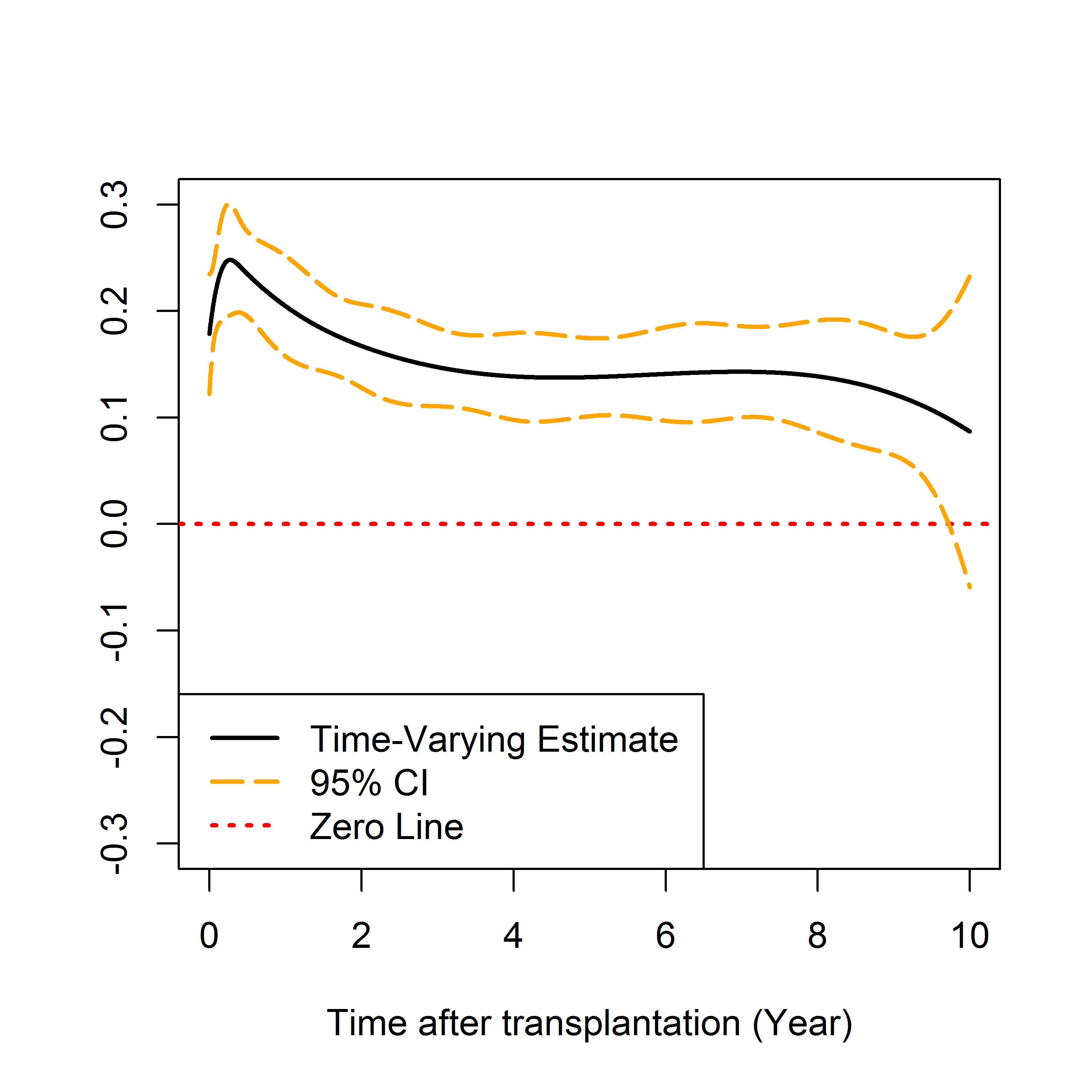
(d) Stroke

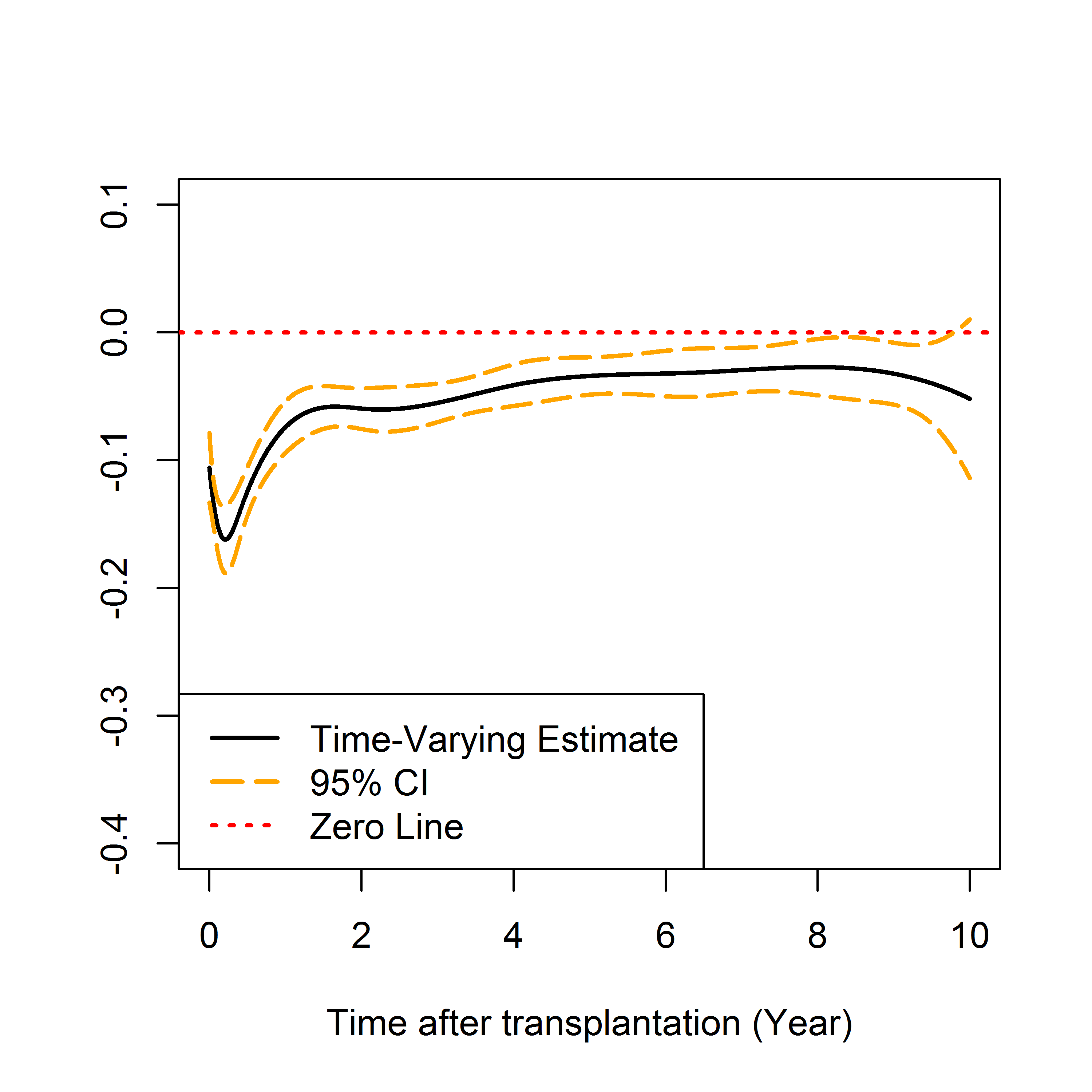
(e) HLA Match

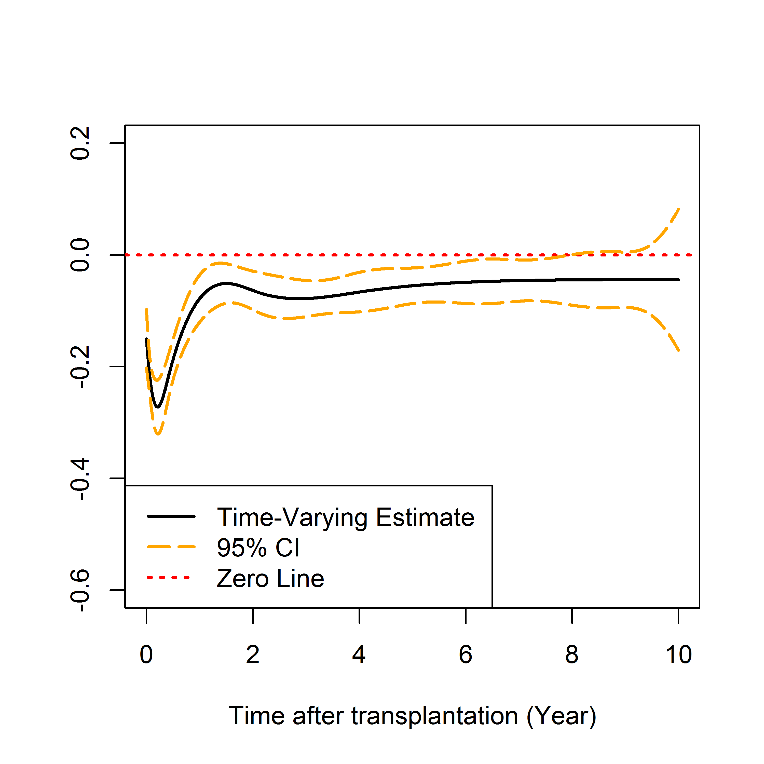
(f) Drug Treated Hypertension

Figure 7: Transplant data: estimated coefficients (solid lines) and 95% confidence interval (dashed lines) for time-varying effects.

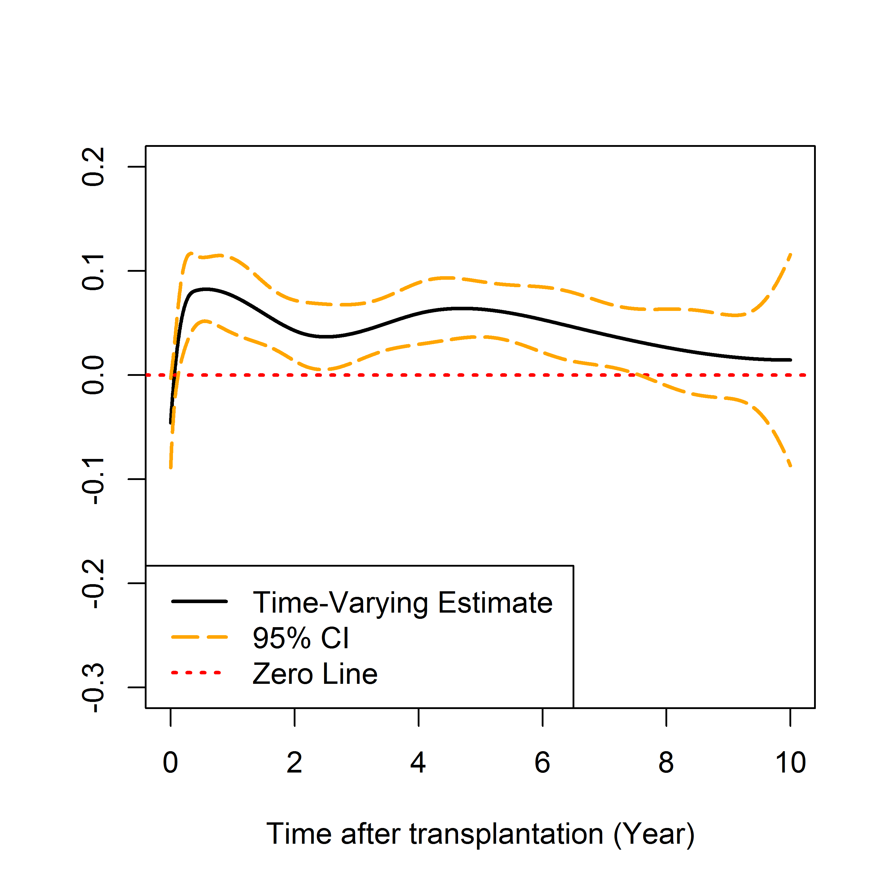
(a) Male

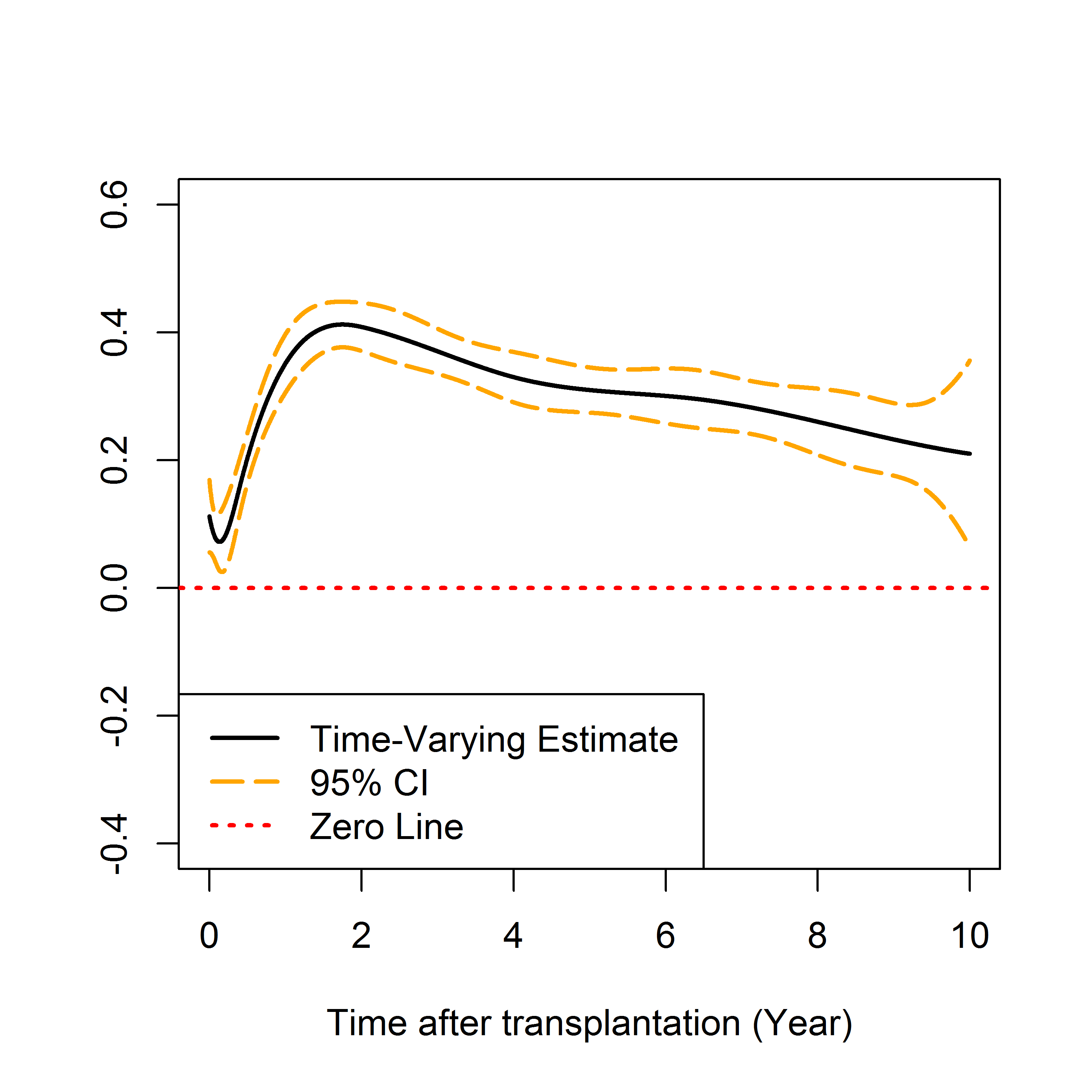
(b) African American

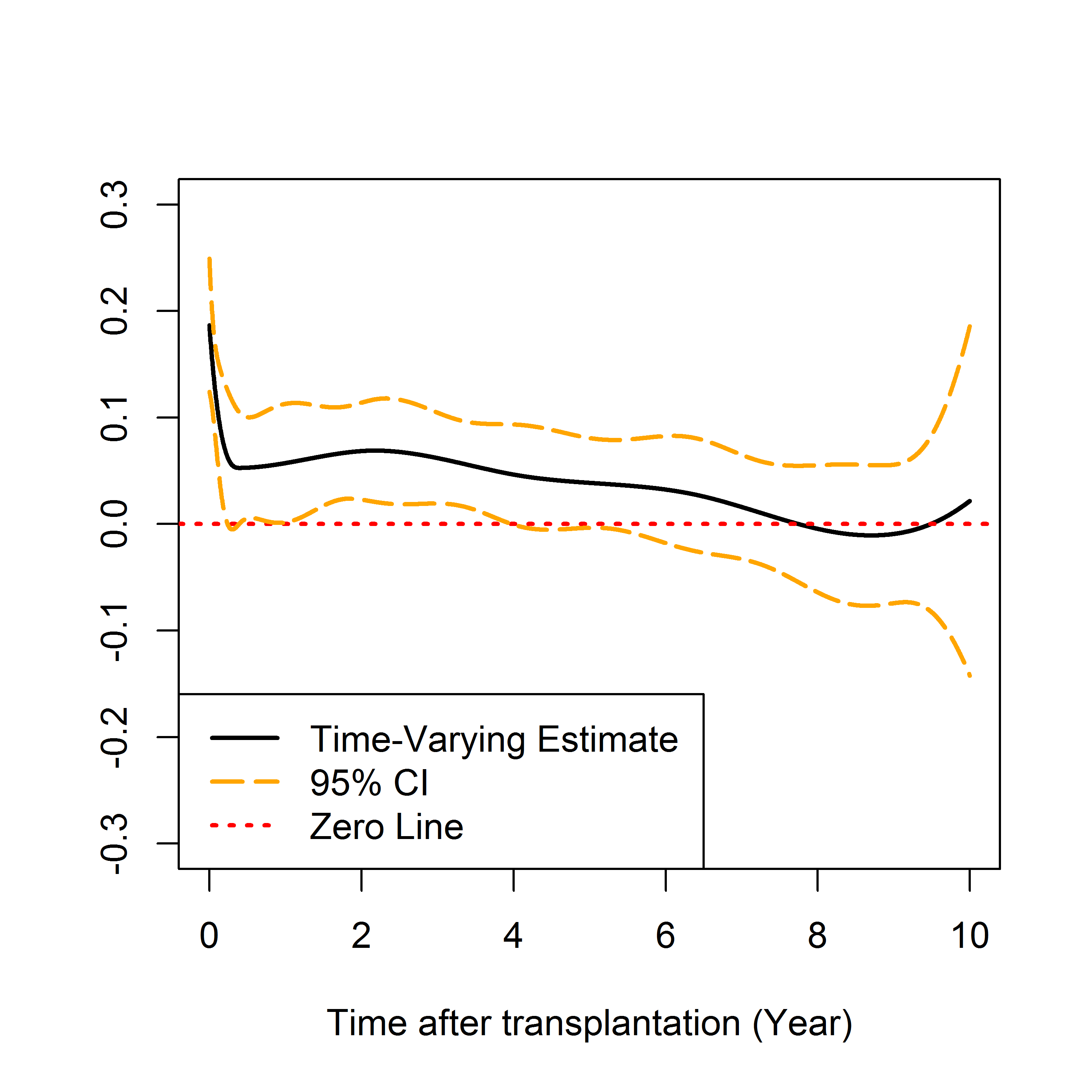
(c) Recipient Other Therapies

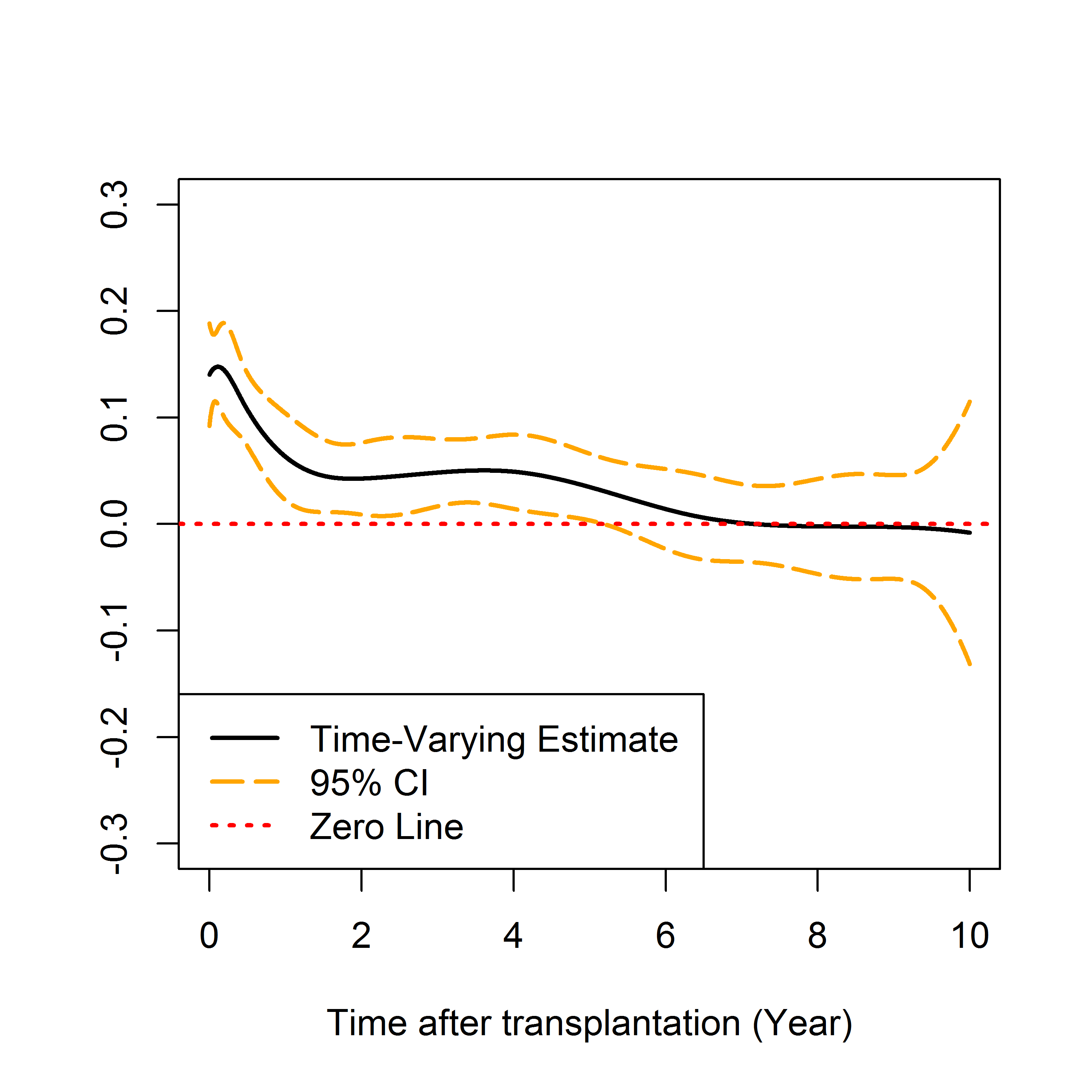
(d) High Cold Ischemic Time

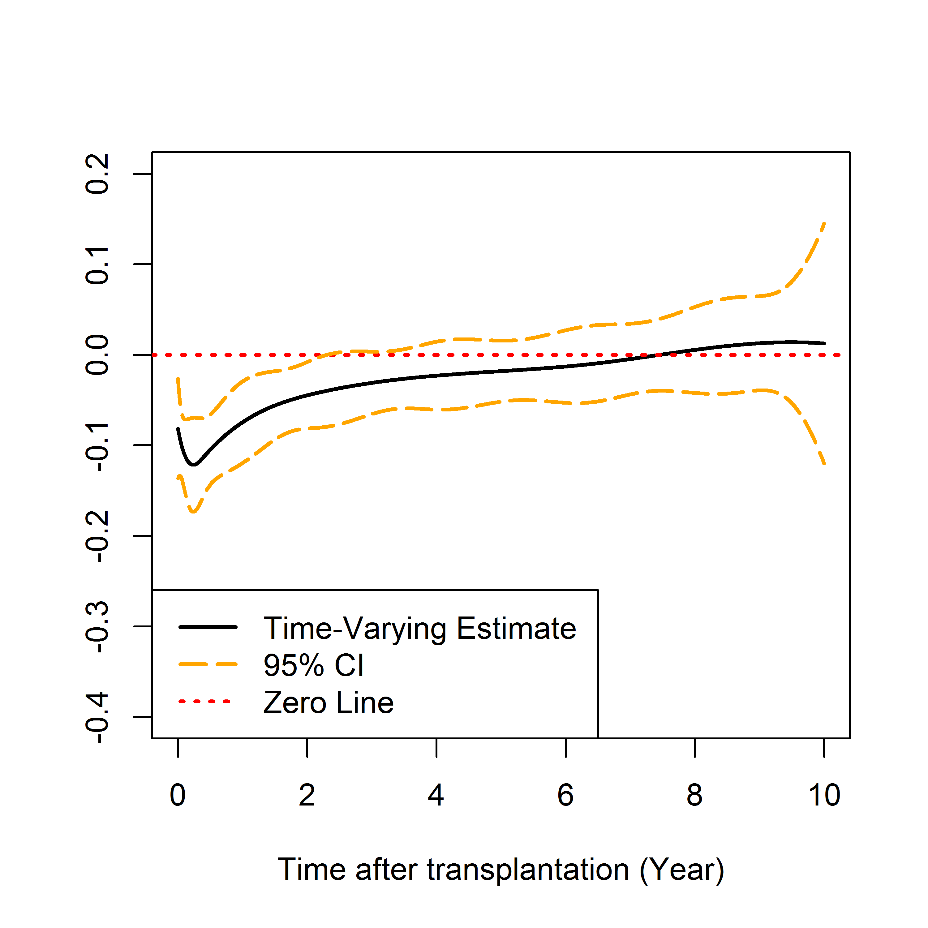
(e) Donor Height

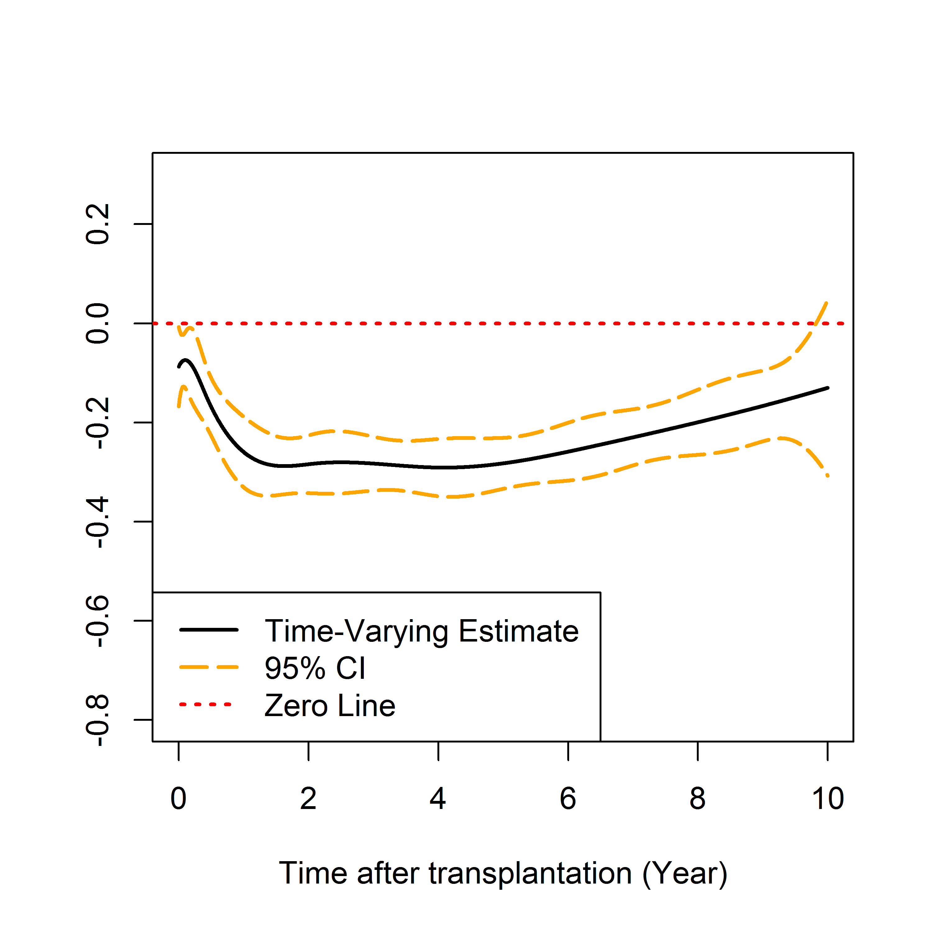
(f) Polycystic Kidney Disease

5 Discussion

Detecting and accounting for time-varying effects are particularly important in the context of clinical studies, as non-proportional hazards have already been reported in the clinical literature [6, 7]. However, in survival analysis, the computational burden to model time-varying effects increases quickly as the sample size or the number of predictors grows. In this report, we propose a Minorization-Maximization-based steepest ascent method. Our procedure iteratively updates the optimal block-wise direction along which the directional derivative is maximized and, hence, the approximate increase in log-partial likelihood is greatest. Our approach is a computationally simple technique, which extends existing boosting methods to estimate time-varying effects for time-to-event data. Numerical studies suggest that the proposed method provides feasible and accurate estimates for large-scale settings.

The proposed method can be extended to high-dimensional settings with the number of predictors larger than the sample size. Since only one variable is updated at each MMSA iteration, variable selection can be achieved by using a finite number of boosting iterations, which can be determined by cross-validation. Compared with penalized methods, the MMSA is flexible and easily implemented without the need to apply constrained optimizations. The resulting approach simultaneously selects and automatically determines potential time-varying effects in high-dimensional time-to-event data. We will report this work in another report.

Appendix A

Proof of Proposition 1

Consider a second-order Taylor expansion,

$$\ell(\boldsymbol{\theta})=\ell(\boldsymbol{\widehat{\theta}})+\triangledown\ell(\widehat{\boldsymbol{\theta}})^{T}(\boldsymbol{\theta}-\boldsymbol{\widehat{\theta}})+\frac{1}{2}(\boldsymbol{\theta}-\boldsymbol{\widehat{\theta}})^{T}\triangledown^{2}\ell(\widetilde{\boldsymbol{\theta}})(\boldsymbol{\theta}-\boldsymbol{\widehat{\theta}}),$$

where $\widetilde{\boldsymbol{\theta}}$ lies between $\boldsymbol{\theta}$ and $\boldsymbol{\widehat{\theta}}$. Assuming $\mathbf{H}(\boldsymbol{\theta})$ is positive definite, we have,

$$\lambda_{max}\left(\{\mathbf{H}(\boldsymbol{\widehat{\theta}})\}^{-1/2}\{-\triangledown^{2}\ell(\boldsymbol{\widetilde{\theta}})\}\{\mathbf{H}(\boldsymbol{\widehat{\theta}})\}^{-1/2}\right)=\lambda_{max}\left(\{\mathbf{H}(\boldsymbol{\widehat{\theta}})\}^{-1}\{-\triangledown^{2}\ell(\boldsymbol{\widetilde{\theta}})\}\right),$$

and for all $\boldsymbol{\theta}\neq\boldsymbol{\widehat{\theta}}$

$$\lambda_{max}\left(\{\mathbf{H}(\boldsymbol{\widehat{\theta}})\}^{-1}\{-\triangledown^{2}\ell(\boldsymbol{\widetilde{\theta}})\}\right)\geq\frac{(\boldsymbol{\theta}-\boldsymbol{\widehat{\theta}})^{T}(-\triangledown^{2}\ell(\boldsymbol{\widetilde{\theta}}))(\boldsymbol{\theta}-\boldsymbol{\widehat{\theta}})}{(\boldsymbol{\theta}-\boldsymbol{\widehat{\theta}})^{T}\mathbf{H}(\boldsymbol{\widehat{\theta}})(\boldsymbol{\theta}-\boldsymbol{\widehat{\theta}})}.$$

Thus, if $\lambda_{max}\left(\{\mathbf{H}(\boldsymbol{\widehat{\theta}})\}^{-1/2}\{-\triangledown^{2}\ell(\boldsymbol{\widetilde{\theta}})\}\{\mathbf{H}(\boldsymbol{\widehat{\theta}})\}^{-1/2}\right)<1/\nu,$ we have

$${}(\boldsymbol{\theta}-\boldsymbol{\widehat{\theta}})^{T}(-\triangledown^{2}\ell(\boldsymbol{\widetilde{\theta}}))(\boldsymbol{\theta}-\boldsymbol{\widehat{\theta}})<\frac{1}{\nu}(\boldsymbol{\theta}-\boldsymbol{\widehat{\theta}})^{T}\mathbf{H}(\boldsymbol{\widehat{\theta}})(\boldsymbol{\theta}-\boldsymbol{\widehat{\theta}}).$$

It follows that $\ell(\boldsymbol{\theta})\geq g(\boldsymbol{\theta}|\widehat{\boldsymbol{\theta}})$ for all $\boldsymbol{\theta}$.

Proof of Proposition 2

To assess the numerical convergence of the MMSA algorithm, we follow the strategy in Lange [26] and define the following concepts:

1. A point $\boldsymbol{\theta}$ is a cluster point of a sequence $\boldsymbol{\widehat{\theta}}^{(m)}$ if every neighborhood of $\boldsymbol{\theta}$ (i.e., a subset that includes an open set containing $\boldsymbol{\theta}$) contains infinitely many $\boldsymbol{\widehat{\theta}}^{(m)}$.

2. A point $\boldsymbol{\theta}$ is a fixed point if $\boldsymbol{\theta}=M(\boldsymbol{\theta})$, where $M(\boldsymbol{\theta})$ is the iteration map generated by the MMSA algorithm.

The following steps provide the ground for the proof of Proposition 2.

Step 1 The fixed points of iteration map $M(\boldsymbol{\theta})$ generated by the MMSA algorithm, and the stationary points of the objective function $\ell(\boldsymbol{\theta})$ coincide.

Recall $\ell(\boldsymbol{\theta})\geq g(\boldsymbol{\theta}|\boldsymbol{\widehat{\theta}}^{(m-1)})$ for all $\boldsymbol{\theta}$, and $g(\boldsymbol{\widehat{\theta}}^{(m-1)}|\boldsymbol{\widehat{\theta}}^{(m-1)})=\ell(\boldsymbol{\widehat{\theta}}^{(m-1)})$. Thus, $\boldsymbol{\widehat{\theta}}^{(m-1)}$ is a stationary point of the difference $g(\boldsymbol{\theta}|\boldsymbol{\widehat{\theta}}^{(m-1)})-\ell(\boldsymbol{\theta})$. The following gradient identity holds

$$\nabla g(\boldsymbol{\widehat{\theta}}^{(m-1)}|\boldsymbol{\widehat{\theta}}^{(m-1)})=\nabla\ell(\boldsymbol{\widehat{\theta}}^{(m-1)}).$$

By Condition (A), $M(\boldsymbol{\widehat{\theta}}^{(m-1)})=\boldsymbol{\widehat{\theta}}^{(m-1)}$ if and only if $\nabla g(\boldsymbol{\widehat{\theta}}^{(m-1)}|\boldsymbol{\widehat{\theta}}^{(m-1)})=\nabla\ell(\boldsymbol{\widehat{\theta}}^{(m-1)})=0.$ Therefore, the fixed points of iteration map $M(\boldsymbol{\theta})$ and the stationary points of $\ell(\boldsymbol{\theta})$ coincide.

Step 2 Every cluster point of iterates $\boldsymbol{\widehat{\theta}}^{(m)}=M(\boldsymbol{\widehat{\theta}}^{(m-1)})$ generated by the iteration map $M(\boldsymbol{\theta})$ of the MMSA algorithm is a stationary point of $\ell(\boldsymbol{\theta})$. Furthermore, the set of stationary points $\mathcal{F}$ is closed and the limit of the following distance function is zero:

$$\lim_{m\rightarrow\infty}\inf_{\boldsymbol{\theta}\in\mathcal{F}}||\boldsymbol{\widehat{\theta}}^{(m)}-\boldsymbol{\theta}||_{2}=0.$$

By the coercive condition assumed in Condition (B), the sequence $\boldsymbol{\widehat{\theta}}^{(m)}$ is contained within the compact super-level set $\{\boldsymbol{\theta}\in\mathcal{U}:\ell(\boldsymbol{\theta})\geq\ell(\boldsymbol{\theta}_{0})\},$ for some $\boldsymbol{\theta}_{0}\in\mathcal{U}$. Existence of a cluster point is then guaranteed by the compactness of the super-level set. Consider a cluster point $\boldsymbol{\widetilde{\theta}}=\lim_{r\rightarrow\infty}\boldsymbol{\widehat{\theta}}^{(m_{r})}$. The ascent property in Proposition 1 guarantees that $\lim_{r\rightarrow\infty}\ell(\boldsymbol{\widehat{\theta}}^{(m_{r})})$ exists. Moreover, the continuity of $M(\boldsymbol{\theta})$ and $\ell(\boldsymbol{\theta})$ imply

$$\lim_{r\rightarrow\infty}\ell(\boldsymbol{\widehat{\theta}}^{(m_{r})})=\ell(\lim_{r\rightarrow\infty}\boldsymbol{\widehat{\theta}}^{(m_{r})}).$$

Using the ascent property once again,

$$\ell(M(\boldsymbol{\widetilde{\theta}}))\geq g(M(\boldsymbol{\widetilde{\theta}})|\boldsymbol{\widetilde{\theta}})\geq g(\boldsymbol{\widetilde{\theta}}|\boldsymbol{\widetilde{\theta}})=\ell(\boldsymbol{\widetilde{\theta}}).$$

Note that the ascent property and the fact that $\ell(\boldsymbol{\widetilde{\theta}})$ is the supremum of $\ell(\boldsymbol{\widehat{\theta}}^{(m_{r})})$ imply that $\ell(\boldsymbol{\widetilde{\theta}})=\ell(M(\boldsymbol{\widetilde{\theta}}))$. Thus, equality holds throughout the inequality above and hence

$$g(M(\boldsymbol{\widetilde{\theta}})|\boldsymbol{\widetilde{\theta}})=g(\boldsymbol{\widetilde{\theta}}|\boldsymbol{\widetilde{\theta}}).$$

By Condition (A), $M(\boldsymbol{\widetilde{\theta}})=\boldsymbol{\widetilde{\theta}}$, e.g. the cluster point $\boldsymbol{\widetilde{\theta}}$ is also a fixed point. Results in step 1 then imply that the fixed point $\boldsymbol{\widetilde{\theta}}$ is also a stationary point of $\ell(\boldsymbol{\theta})$.

To show that the set of stationary points $\mathcal{F}$ is closed, suppose there exists a sub-sequence $\boldsymbol{\widehat{\theta}}^{(m_{r})}\in\mathcal{F}$ and $\lim_{r\rightarrow\infty}\boldsymbol{\widehat{\theta}}^{(m_{r})}=\boldsymbol{\widetilde{\theta}}$. By the continuity of $M(\boldsymbol{\theta})$, we have $\lim_{r\rightarrow\infty}M(\boldsymbol{\widehat{\theta}}^{(m_{r})})=M(\boldsymbol{\widetilde{\theta}})$, where $M(\boldsymbol{\widehat{\theta}}^{(m_{r})})=\boldsymbol{\widehat{\theta}}^{(m_{r})}$ by the definition of $\mathcal{F}$. It follows that $\lim_{r\rightarrow\infty}\boldsymbol{\widehat{\theta}}^{(m_{r})}=M(\boldsymbol{\widetilde{\theta}})$ and $M(\boldsymbol{\widetilde{\theta}})=\boldsymbol{\widetilde{\theta}}$. Thus, the set of stationary points $\mathcal{F}$ is closed. To show

$$\lim_{m\rightarrow\infty}\inf_{\boldsymbol{\theta}\in\mathcal{F}}||\boldsymbol{\widehat{\theta}}^{(m)}-\boldsymbol{\theta}||_{2}=0,$$

we assume on the contrary there exist an $\varepsilon>0$ and a sequence $\boldsymbol{\widehat{\theta}}^{(m_{r})}$ with $||\boldsymbol{\widehat{\theta}}^{(m_{r})}-\boldsymbol{\theta}||_{2}\geq\varepsilon$ for all $m_{r}$. By the compactness and taking a convergent subsequence, we have a cluster point outside of $\mathcal{F}$, which contradicts the definition of $\mathcal{F}$.

Finally, if the observed information matrix $-\triangledown^{2}\ell(\boldsymbol{\theta})$ is positive definite in the super-level set, any sequence of $\boldsymbol{\widehat{\theta}}^{(m)}$ possesses a limit, and this limit is a stationary point of $\ell(\boldsymbol{\theta})$.

References

- [1] Boyd, S. and Vandenberghe, L. (2004). Convex Optimization, Cambridge University Press, New York.
- [2] Breiman, L. (1999). Prediction games and arcing algorithms. Neural Computation 11 1493–1517.
- [3] Bühlmann, P. and Yu, B. (2003). Boosting with the loss: Regression and classification. Journal of the American Statistical Association 98(462) 324–339.
- [4] Bühlmann, P. and Yu, B. (2006). Boosting for high-dimensional linear models. Annals of Statistics 34 559–583.
- [5] Cox, D.R. (1972). Regression models and life tables (with Discussion). Journal of the Royal Statistical Society, Series B 34 187–200.
- [6] Dekker, F.W. and Mutsert, R. and Dijk, P.C. and Zoccali, C. and Jager, K.J. (2008). Survival analysis: time-dependent effects and time-varying risk factors. Kidney International, 74 994–997.
- [7] Englesbe, M.J. and Lee, J.S. and Lee, J.S. and He, K. and Fan, L. and Schaubel, D.E. and Schaubel, D.E. and Sheetz, K.H. and Harbaugh, C.M. and Holcombe, S.A. and Campbell, D.A. and Sonnenday, C.J. and Wang, S.C. (2012). Analytic morphomics, core muscle size, and surgical outcomes. Annals of Surgery 256(2) 255–261.
- [8] Friedman, J. and Hastie, T. and Tibshirani, R. (2010). Regularization paths for generalized linear models via coordinate descent. Journal of Statistical Software 33(1) 1–22.
- [9] Freund, Y. and Schapire, R. (1996). Experiments with a new boosting algorithm. Machine Learning: Proceedings of the Thirteenth International Conference, Morgan Kauffman, San Francisco, 74 148–156.
- [10] Friedman, J.H. and Hastie, T. and Tibshirani, R. (2000). Additive logistic regression: A statistical view of boosting (with discussion). Annals of Statistics 28(2) 337–407.
- [11] Friedman, J.H. (2001). Greedy function approximation: A gradient boosting machine. Annals of Statistics 29(5) 1189–1232.
- [12] Friedman, J.H. (2002). Stochastic Gradient Boosting. Computational Statistics and Data Analysis 38(4) 367–378.
- [13] Frohnert, P.P. and Donadio, J.V.Jr and Velosa, J.A. and Holley, K.E. and Sterioff, S. (1997). The fate of renal transplants in patients with IgA nephropathy. Clinical Transplant 11(2) 127–133.
- [14] Grambsch, P. and Therneau, T. (1994). Proportional hazards tests and diagnostics based on weighted residuals. Biometrika 81 515–526.
- [15] Gray, R.J. (1992). Flexible methods for analyzing survival data using splines, with applications to breast cancer prognosis. Journal of the American Statistical Association 87(420) 942–951.
- [16] Gray, R.J. (1994). Spline-based tests in survival analysis. Biometrics 50(3) 640–652.
- [17] Hadimeri, H. and Norden, G. and Friman, S. and Nyberg, G. (1997). Autosomal dominant polycystic kidney disease in a kidney transplant population. Nephrol Dial Transplant 12 1431–1436.
- [18] Hastie, T. and Tibshirani, R. (1993). Varying-coefficient models. Journal of the Royal Statistical Society, Series B 55 757–796.
- [19] He, K. and Li, Y.M. and Wei, Q.Y. and Li, Y. (2017). Computationally efficient approach for modeling complex and big survival data. Big and Complex Data Analysis: Statistical Methodologies and Applications, Edited volume by Springer 193-207.
- [20] He, K. and Yang, Y. and Li, Y.M. and Zhu, J. and Li, Y. (2017). Modeling time-varying effects with large-scale survival data: an efficient quasi-Newton approach. Journal of Computational and Graphical Statistics 26(3) 635-645.
- [21] He, K. and Li, Y.M. and Zhu, J. and Liu, H.L. and Lee, J.E. and Amos, C.I. and Hyslop, T. and Jin, J.S. and Lin, H.Z. and Wei, Q.Y. and Li, Y. (2016). Component-wise gradient boosting and false discovery control in survival analysis with high-dimensional covariates. Bioinformatics 32(1) 50-57.
- [22] Hofner, B. and Hothorn, T. and Kneib, T. (2008). Variable selection and model choice in survival models with time-varying effects. Technical Report Department of Statistics, University of Munich.
- [23] Honda, T. and Härdle, W.K. (2014). Variable selection in Cox regression models with varying coefficients. Journal of Statistical Planning and Inference 148 67–81.
- [24] Kalantar-Zadeh, K. (2005). Causes and consequences of the reverse epidemiology of body mass index in dialysis patients. Journal of Renal Nutrition 15 142–147.
- [25] Kalbfleisch, J.D. and Wolfe, R.A. (2013). On Monitoring Outcomes of Medical Providers. Statistics in Biosciences 2 286–302.
- [26] Lange, K. (2012). Optimization, 2nd ed. Springer, New York.
- [27] Liu, M. and Lu, W. and Shore, R. E. and Zeleniuch-Jacquotte, A. (2010). Cox regression model with time-varying coefficients in nested case-control studies. Biostatistics 11(4) 693–706.
- [28] Mason, L. and Baxter, J. and Bartlett, P.r and Frean, M. (1999). Boosting algorithms as gradient descent in function space. In Advances in Large Margin Classifiers. MIT Press.
- [29] Meier-Kriesche, H.U. and Port, F.K. and Ojo, A.O. and Rudich, S.M. and Hanson, J.A. and Cibrik, D.M. and Leichtman, A.B. and Kaplan, B. (2000). Effect of waiting time on renal transplant outcome. Kidney International 58(3) 1311–1317.
- [30] Muntean, A. and Lucan, M. (2013). Immunosuppression in kidney transplantation. Clujul Medical 86 177–180.
- [31] Perperoglou, A. and le Cessie, S. and van Houwelingen, H.C. (2006). A fast routine for fitting Cox models with time varying effects of the covariates. Computer Methods and Programs in Biomedicine 25 154–161.
- [32] Phelan, P.J. and Shields, W. and O’Kelly, P. and Pendergrass, M. and Holian, J. and Walshe, J. and Magee, C. and Little, D. and Hickey, D. and Conlon, P.J. (2009). Left versus right deceased donor renal allograft outcome. Transplant International 25 1159–1163.
- [33] Ridgeway, G. (1999). The State of Boosting. Computing Science and Statistics 31 172–181.
- [34] Rozanski, J. and Kozlowska, I. and Myslak, M. (2005). Pretransplant nephrectomy in patients with autosomal dominant polycystic kidney disease. Transplant Proc 37 666–668.
- [35] Ruder, S. (2016). An overview of gradient descent optimization algorithm. arXiv preprint
- [36] Saran, R. and Robinson, B. and Abbott, K.C. et al. (2018). US Renal Data System 2017 Annual Data Report: Epidemiology of Kidney Disease in the United States. American Journal of Kidney Diseases 71(3) S1–S672.
- [37] Tian, L. and Zucker, D. and Wei, L. (2005). On the Cox Model with Time-Varying Regression Coefficients. Journal of the American Statistical Association 100(469) 72–183.
- [38] Therneau, T.M. and Grambsch, P.M. (2000). Modeling Survival Data: Extending the Cox Model, Springer, New York.
- [39] Verweij, P.J.M. and van Houwelingen, H.C. (1993). Cross-validation in survival analysis. Statistics in Medicine 12 2305–2314.
- [40] Wolfson, J. (2011). EEBoost: A general method for prediction and variable selection based on estimating equations. Journal of the American Statistical Association 106(493) 296–305.
- [41] Xiao, W. and Lu, W. and Zhang, H.H. (2016). Joint structure selection and estimation in the time-varying coefficient Cox model. Statistica Sinica 26(2) 547–567.
- [42] Yan, J. and Huang, J. (2012). Model selection for Cox models with time-varying coefficients. Biometrics 68(2) 419–428.
- [43] Zou, H. (2006). The adaptive lasso and its oracle properties. Journal of the American Statistical Association 101(476) 1418–1429.
- [44] Zhang, H. and Lu, W. (2006). Adaptive lasso for Cox’s proportional hazards model. Biometrika 94 691–703.
- [45] Zucker, D.M. and Karr, A.F. (1990). Nonparametric survival analysis with time-dependent covariate effects: a penalized partial likelihood approach. Annals of Statistics 18(1) 329–353.