Colliding Winds in and around the Stellar Group IRS 13E at the Galactic Center

Abstract

IRS 13E is an enigmatic compact group of massive stars located in projection only 3$\aas@@fstack{\prime\prime}$6 away from Sgr A*. This group has been suggested to be bounded by an intermediate-mass black hole (IMBH). We present a multi-wavelength study of the group and its interplay with the environment. Based on Chandra observations, we find the X-ray spectrum of IRS 13E can be well characterized by an optically thin thermal plasma. The emission peaks between two strongly mass-losing Wolf-Rayet stars of the group. These properties can be reasonably well reproduced by simulated colliding winds of these two stars. However, this scenario under-predicts the X-ray intensity in outer regions. The residual emission likely results from the ram-pressure confinement of the IRS 13E group wind by the ambient medium and is apparently associated with a shell-like warm gas structure seen in Pa-alpha and in ALMA observations. These latter observations also show strongly peaked thermal emission with unusually large velocity spread between the two stars. These results indicate that the group is colliding with the bar of the dense cool gas mini-spiral around Sgr A*. The extended X-ray morphology of IRS 13E and its association with the bar further suggest that the group is physically much farther away than the projected distance from Sgr A*. The presence of an IMBH, while favorable to keep the stars bound together, is not necessary to explain the observed stellar and gas properties of IRS 13E.

1 Introduction

The Galactic center (GC) of the Milky Way is a unique site for the detailed study of a multitude of complex astrophysical phenomena that appear common to the nuclear regions of many galaxies. Multiple stellar populations and structures have been identified around Sgr A* – the supermassive black hole (SMBH) of our Galaxy (e.g., Paumard et al., 2006; Bartko et al., 2009; Schödel et al., 2014). Massive stars, in particular, appear to form such perplexing structures as the clock-wise disk (CWD) and possibly a counter-clock-wise disk (CCWD). In addition, a compact group of massive stars, IRS 13E, has long been recognized and may or may not belong to the CCWD (Genzel et al., 2010). The formation and dynamics of these distinct massive star structures, as well as their interplay with the gaseous environment and Sgr A*, have been an active research topic for many years (e.g., Nayakshin et al., 2007; Cuadra et al., 2008).

Here we focus on IRS 13E, which is located only 3$\aas@@fstack{\prime\prime}$6 (1”=0.039 pc at our adopted GC distance $D=8$ kpc) in projection away from Sgr A*, compared with its Bondi radius of 4” for hot gas accretion (Wang et al., 2013). This apparent proximity to Sgr A* makes the group particularly interesting and puzzling (e.g., Fig. 1A). Within a radius of 0$\aas@@fstack{\prime\prime}$27, the group contains two Wolf-Rayet (WR) stars (E2 – WN8 and E4 or more precisely E4.0 – WC9) and one OB supergiant (E1), as well as numerous red objects, including E3, which has been resolved into no less than six stable components (e.g., Fritz et al., 2010). The three confirmed massive stars, sharing similar proper motions and line-of-sight (LoS) velocities (Table 1), appear to be gravitationally bound. But the total stellar mass of the stars ($\sim 350{\rm~{}M_{\odot}}$ according to Paumard et al. 2006 or up to $\sim 2000{\rm~{}M_{\odot}}$ to Fritz et al. 2010) is apparently far too little to overcome the strong tidal force of Sgr A*, if the projected separation approximately represents the physical one. The required self-gravitating mass indicates the presence of an embedded intermediate-mass black hole (IMBH), with a mass $M_{IMBH}\lower 2.0pt\hbox{$\,\buildrel\scriptstyle>\over{\scriptstyle\sim}\,$}10^{3}{\rm~{}M_{\odot}}$ (Maillard et al., 2004) and possibly as large as several $10^{4}{\rm~{}M_{\odot}}$ (Schödel et al., 2005), and/or many stellar-mass ones (Fritz et al., 2010; Banerjee & Kroupa, 2011). This upper bound mass is obtained from the existing limits on the proper motion acceleration of stars in IRS 13E and on the reflex motion of Sgr A* (Fritz et al., 2010).

Interestingly, an IMBH of $2.4\times 10^{4}~{}{\rm M}_{\sun}$ has recently been proposed to be responsible for the large velocity width ($\sim 650{\rm~{}km~{}s^{-1}}$) of the spatially resolved ionized gas detected at IRS 13E 3.0 (Tsuboi et al., 2017b, 2019). Whether or not such an IMBH is present in the group has strong implications for understanding the gas and stellar dynamics in the GC, as well as IRS 13E itself (Portegies Zwart et al., 2006). We find that the large velocity width, as well as some other outstanding features in and around IRS 13E, may alternatively and naturally be explained by the collision of the fast stellar winds from the group with its ambient medium. The group wind can then be partially confined by the ram-pressure of the collision, while dense blobs are compressed, evaporated and stripped, forming gas flows of high density and velocity spread as observed. Furthermore, the dispersed cool gas, as well as the IRS 13E wind, can be an important source of mass and/or ram-pressure in the vicinity of Sgr A* (Melia & Falcke, 2001; Paumard et al., 2001; Mościbrodzka et al., 2006; Cuadra et al., 2008), affecting the gas dynamics around the SMBH and even its accretion. Here we attempt to address these issues about the nature of IRS 13E and its interplay with the environment, based on hydrodynamic simulations and multi-wavelength observations.

Table 1: Velocities of objects in IRS 13E

object	$v_{\rm RA}$	$v_{\rm Decl.}$	$v_{z}$	$v_{\rm T}$
E1	-142.5	-105.5	134$\pm 10$	222
E2	-249.2	23	65 $\pm 30$	259
E3.0	-82	8	-23	86
E4	-227	26	200$\pm 200$	304
$\bar{v}_{E2+4}$	-238	25	$68\pm 30$	249
$v_{bar}$	-150	64	-30	166
$v_{r}=\bar{v}_{E2+4}-v_{bar}$	-88	-39	98	137

Note: The velocities are in units of ${\rm~{}km~{}s^{-1}}$. The measurements for E1-4 are from Table 1 and Appendix B of Fritz et al. (2010). Quoted errors for the transverse components $v_{\rm RA}$ and $v_{\rm Decl.}$ are not included because they are negligible compared to other uncertainties; $v_{\rm T}$ is the derived total velocity of each object. The average velocity ($\bar{v}_{E2+4}$) of the two energetically dominant stars, E2 and E4, is assumed as the effective velocity of IRS 13E. While the LoS component ($v_{z}$) of the bar velocity ($v_{bar}$) is estimated with the ALMA data presented here (see § 6.2, in particular Figs. 8 and 9), the $v_{\rm RA}$ and $v_{\rm Decl.}$ components are with the mean VLA-measured proper motion of gas local to IRS 13E (see § 8.1), together with the position angle of 25^∘ of the bar (Liszt, 2003).

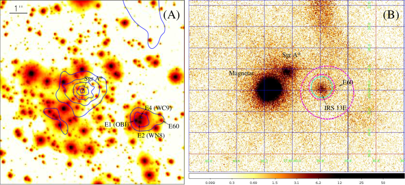
Figure 1: X-ray views of the IRS 13E and Sgr A* region: (A) Overlaid on the K-band image from VLT/NACO are X-ray (blue) contours at 2, 4, 8, 16, and 32 $\times 10^{-4}{\rm~{}cts~{}s^{-1}~{}arcsec^{-2}}$, which are obtained from the Chandra/ACIS-S/HETG 0th-order intensity image constructed in the 1-9 keV range and adaptively smoothed with CSMOOTH with a signal-to-noise ratio of 2.5-3.5. (B) An unsmoothed X-ray image of the region from later ACIS-S observations with no grating; the brightest source, 2$\aas@@fstack{\prime\prime}$4 southeast of Sgr A*, in the image is the magnetar SGR J1745-2900, which was not active during the period when the data in (A) were taken (Mori et al., 2013). The spectral extraction regions for IRS 13E and its background are outlined by the circle of 1^′′ radius (colored in cyan) and the asymmetric annuli (magenta) around IRS 13E. North is up and East is to the left for all the presented images throughout the paper.

We start with an analysis of Chandra observations on IRS 13E. The group is a known X-ray source (Baganoff et al., 2001). Wang et al. (2006) have shown that its emission is extended in a Chandra image and that its X-ray spectrum is hard, inconsistent with what is expected from individual massive stars, but typical for colliding-wind (CW) binaries (Coker & Pittard, 2000; Coker et al., 2002). However, many questions remain unanswered: What may be the morphology of the extended emission, if confirmed? What is the true nature of the emission? Is there any evidence for an accreting BH? Could it really be produced by the stars well separated spatially in IRS 13E? What can we learn about the interplay between IRS 13E and its environment from the properties of the X-ray emission? To address such questions, we conduct a systematic spatial and spectral analysis of the X-ray emission from IRS 13E, based on the archival Chandra observations with a total of 5.3 Ms exposure time, as reported here. We further perform hydrodynamic simulations to check the consistency of the interpretation of the X-ray emission as being due to the CW (Coker & Pittard, 2000; Coker et al., 2002). In the process, we also provide useful constraints on relevant parameters of IRS 13E.

To explore the interplay between IRS 13E and its environment, we also analyze a set of ALMA observations, as well as relevant results from the literature (e.g., Liszt, 2003; Zhao et al., 2009; Fritz et al., 2010; Eckart et al., 2013; Tsuboi et al., 2017b, a, 2019). This analysis allows us to better assess the quality of the ALMA data and to use them in examining various hypotheses, as well as testing our group wind collision scenario.

The organization of the paper is as follows: After a brief description of the X-ray data and their reduction in § 2, we present our detailed analysis and results in § 3, discuss constraints on the X-ray emission from the putative IMBH in § 4, and compare our observational results with the simulations in § 5. We describe the ALMA data analysis and results in § 6. We further present a critical analysis of existing multi-wavelength results and interpretations in § 7, before moving on to test our group wind collision scenario and to explore its implications in § 8. Finally in § 9, we summarize our results and conclusions.

2 Chandra Observations and Data Reduction

The Chandra observations used in the present work can be divided into three sets. The first set, consisting of 45 separate observations (1.5 Ms total exposure) taken before 2012, had the Advanced CCD Imaging Spectrometer-Imaging (ACIS-I) on axis. The second set of 38 observations (3 Ms total) taken during February 6 to October 29, 2012 were from the X-ray Visionary Project (XVP) of Sgr A*, which utilized the High Energy Transmission Gratings (HETG) in combination with the Advanced CCD Imaging Spectrometer-Spectroscopy (ACIS-S; only the 0th-order ACIS-S/HETG data are used here). The third set, including 25 observations with the ACIS-S without the grating, were taken after the XVP, but before May 15, 2015. The combination of these observations, pointed within 2’ of Sgr A*, greatly enhances the counting statistics for the present exploration. The different sets of the data are complementary in their qualities. The spectral resolution of the ACIS-S data is about a factor of $\sim 2$ better than that of the ACIS-I observations (which suffered from a severe charge transfer inefficiency and cannot be fully mitigated in software processing). The 0th-order data of the ACIS-S/HETG observations have the longest total exposure and best counting statistics, although the effective collecting area is low compared to the ACIS-S/NONE (without the grating) data, especially at lower energies ($\lower 2.0pt\hbox{$\,\buildrel\scriptstyle<\over{\scriptstyle\sim}\,$}4$ keV). The ACIS-I data, with the effective area considerably higher than that of the ACIS-S at higher energies, provide the most sensitive coverage of the spectrum above the 6.7-keV iron line.

Individual observations in each of the three data sets are reduced via standard CIAO processing routines. We remove time intervals of significant background flares, with count rates deviating more than 3$\sigma$ or a factor of $\lower 2.0pt\hbox{$\,\buildrel\scriptstyle>\over{\scriptstyle\sim}\,$}1.2$ from the mean rate of individual observations, using the light-curve cleaning routine LC$\_$CLEAN. This cleaning, together with a correction for the dead time of the observations, resulted in 1.44 (ACIS-I), 2.92 (ACIS-S/HETG) and 0.82 (ACIS-S/NONE) Ms effective exposures for subsequent analysis. We correct for the relative astrometry of the observations by matching the centroid positions of sources detected within $3^{\prime}$ of Sgr A*, and then align the absolute position to the radio position of Sgr A* [J2000: $RA=17^{h}45^{m}40\aas@@fstack{s}041,Dec=-29^{\circ}00^{\prime}28\aas@@fstack{\prime\prime}12$; Reid & Brunthaler (2004)]. The three data sets with significantly different instrument responses are analyzed separately and allow independent reliability tests of our various measurements. The source detection is the same as detailed in the supplementary material of Wang et al. (2013).

To study the spatial structure of IRS 13E, we need to account for both the point-spread function (PSF) of the instrument and the scattering of the X-ray emission by dust along the line of sight. To do so, we construct an empirical spatial distribution of the X-ray intensity from J174538.05-290022.3, which shows high time-variability and is thus point-like. With a spectrum indicative of strong absorption and projected only 24^′′ west of IRS 13E [see the supplementary material of Wang et al. (2013)], this source should be located at the GC or beyond. The source has a count rate of $5.6{\rm~{}counts~{}ks^{-1}}$ in the ACIS-S/HETG 0th-order image, indicating a slight pile-up effect [two or more photons in a single “readout frame” being registered as a single event, or rejected as a non X-ray event; Davis (2001)]. The pile-up makes the intensity distribution at the centroid of the source a bit flat, but should have negligible effect on the overall distribution. The count rate of the source is much higher in the ACIS-I or ACIS-S/NONE image. The pile-up effect is correspondingly more important, making the source not an appropriate PSF calibrator. Therefore, our spatial analysis is limited to the ACIS-S/HETG (0th-order) data.

3 X-ray Data Analysis and Results

Fig. 1 presents the X-ray intensity images from the ACIS-S/HETG (A) and ACIS-S/NONE (B) observations. In addition to Sgr A* and IRS 13E, there are two discrete X-ray sources that deserve some notes. First, the bright source seen in Panel (B), 2.4” southeast (SE) of Sgr A*, is the magnetar, SGR J1745-2900, which appeared only after 2012 (Mori et al., 2013). Second, the X-ray enhancement at E60 (Paumard et al., 2006), just west of IRS 13E (Fig. 1A), has a hard spectral shape, as indicated by the 4-9 keV to 1-4 keV band intensity ratio, and is apparently due to the CW of this eclipsing binary. It has a short orbital period of 2.28 days and an inclination angle of $\sim 70^{\circ}$, as determined from both spectroscopical and photometric observations (Pfuhl et al., 2014). These observations further suggest that both the primary ($\sim 20$ M_⊙) and the secondary (10 M_⊙) of the binary have similar spectral types (WN7). The binary is unlikely to be bound to IRS 13E. Although the proper motion of E60 (object #376 in Schödel et al., 2009) is consistent with that of IRS 13E, their LoS velocities are substantially different, $\sim 467{\rm~{}km~{}s^{-1}}$ (E60) vs. $\sim 60{\rm~{}km~{}s^{-1}}$ (IRS13E), indicating that the binary may even be not bound to the gravity of Sgr A* (Pfuhl et al., 2014).

3.1 Spatial analysis

As shown in Fig. 1A, the X-ray emission from IRS 13E appears extended and peaks in the middle between the two WR stars, E2 and E4. To be more quantitative, we compare the centroid position of the X-ray peak with those of the two WR stars. We first measure the positions of the stars in the IR image (taken in 2005) and then correct them according to the known proper motions (Paumard et al., 2006), which are about 0$\aas@@fstack{\prime\prime}$05 over a seven year period. We find that the separation of the two stars is 0$\aas@@fstack{\prime\prime}$32, mostly in the N-S direction. The errors in these measurements, as well as the X-ray one, are difficult to quantify exactly and are mostly systematic, but should be smaller than $\sim 0\aas@@fstack{\prime\prime}1$. The X-ray centroid is right in the middle (slightly closer to E4) in the N-S direction, but is about 0$\aas@@fstack{\prime\prime}$15 off to the west.

The extent of the X-ray emission can be appreciated better in Fig. 2A, which compares a radial X-ray intensity profile of IRS 13E with that of the point-like source J174538.05-290022.3. To obtain an upper limit to a potential point source contribution to the emission, we subtract from its image a normalized image of J174538.05-290022.3 (Fig. 2B). This latter image is scaled to minimize the central peak of the resultant image, but not to produce a hole because of the subtraction. The adopted scaling factor corresponds to a subtracted point-like component accounting for 50% of the total emission. This component can then be considered to be the maximum contribution of a central point source, if present. The remaining diffuse emission in the immediate vicinity of IRS 13E has the full size of about 2^′′ with an uncertainty of $\sim 20\%$, accounting for the PSF/dust broadening (see § 5 for more discussion).

The morphology of the X-ray emission is also interesting. The morphology seen in Fig. 2B, however, somewhat depends on how the “point-like” component is removed, particularly the choice of its centroid position. Nevertheless, the emission is qualitatively most extended in the N-S direction on the east side of IRS 13E, which is apparent also in Fig. 1A. The extendness in the E-W direction is also apparent on the east side. The extendness to the west side is uncertain, largely because of the confusion with E60. We see no evidence for physical interaction between this binary and IRS 13E. Overall, the morphology of the emission seems to fan out toward the east, roughly in the opposite direction of the proper motion of IRS 13E (Paumard et al., 2006, and see § 5 for more discussion). https://www.overleaf.com/project/5d40d06389e5832705b14a32

https://www.overleaf.com/project/5d40d06389e5832705b14a32

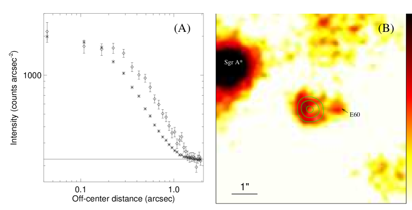
Figure 2: (A) The radial intensity profile of IRS 13E  (diamonds), compared with the profile of the point-like source J174538.05-290022.3 (crosses), all in the ACIS-S/HETG 1-9 keV band. The latter profile has been normalized to the average intensity of the first three bins of the former. This normalization is performed after subtracting the corresponding local background of each profile, estimated as the median value in the 1$\aas@@fstack{\prime\prime}$5-2^′′ range. The profile is then shifted to the local background level (the solid horizontal line) of the IRS 13E profile. (B) A close-up of the ACIS-S/HETG 1-9 keV intensity image of IRS 13E. The intensity is decomposed into extended (color image) and point-like (contour) components. The color bar of the former component is scaled logarithmically in the 0.3-1.5 $\times 10^{3}$ counts arcsec^-2 range (white-black), while the latter component is modeled with the emission from the point-like source, J174538.05-290022.3, and is illustrated as the intensity contours at 0.3, 0.5, 1.0, and 2 $\times 10^{3}$ counts arcsec^-2.

3.2 Spectral analysis

Fig. 3 presents X-ray spectra of IRS 13E, extracted from the three data sets. These spectra are local background-subtracted (see the spectral extraction regions shown in Fig. 1B) and are adaptively grouped to achieve a signal-to-noise ratio greater than 3 per bin. The presence of the S, Ar, and Fe He-$\alpha$ emission lines is apparent, clearly indicating the thermal nature of the spectra. We detect no significant variation in the flux and spectral shape among the spectra, so we fit them jointly, first with an optically thin plasma VAPEC. (Here the spectral models are all in reference to those implemented in the XSPEC software package; Arnaud 1996.) The photoelectric absorption uses the Tuebingen-Boulder model [TBABS; Wilms et al. (2000)] with the cross-sections from Verner et al. (1996). The metal abundance pattern of the plasma and the foreground X-ray-absorbing gas are adopted from Wilms et al. (2000) for the interstellar medium (ISM). This simple model fit is acceptable and gives the best-fit parameters listed in Table 2. In particular, the fitted X-ray absorbing, equivalent hydrogen column density $1.74(1.64-1.94)\times 10^{23}\rm~{}cm^{-2}$ for IRS 13E, which may be compared with $1.66(1.41-1.94)\times 10^{23}\rm~{}cm^{-2}$ for Sgr A* (Wang et al., 2013).

Table 2: X-ray characterization of IRS 13E

Centroid position	$17^{h}45^{m}39\aas@@fstack{s}78$
	$-29^{\circ}0^{\prime}29\aas@@fstack{\prime\prime}7$
Overall size	$\sim 2^{\prime\prime}$
Plasma temperature kT (keV)	1.34 (1.22-1.46)
ISM metal abundancea	1.1(0.83-1.7)
Absorbing column density NrmH ($\times 10^{23}\rm~{}cm^{-2}$)	1.74 (1.64-1.94)
Normalization ($10^{-4}$)	5.0(4.4-6.9)
$L_{1-9\rm~{}keV}({\rm erg~{}s^{-1}})$	1.2$\times$1033
$\chi^{2}/d.o.f.$	314/267

Note: The metal abundances are relative to the interstellar medium (ISM) values given in Wilms et al. (2000). The presented error ranges are at the 90% confidence.

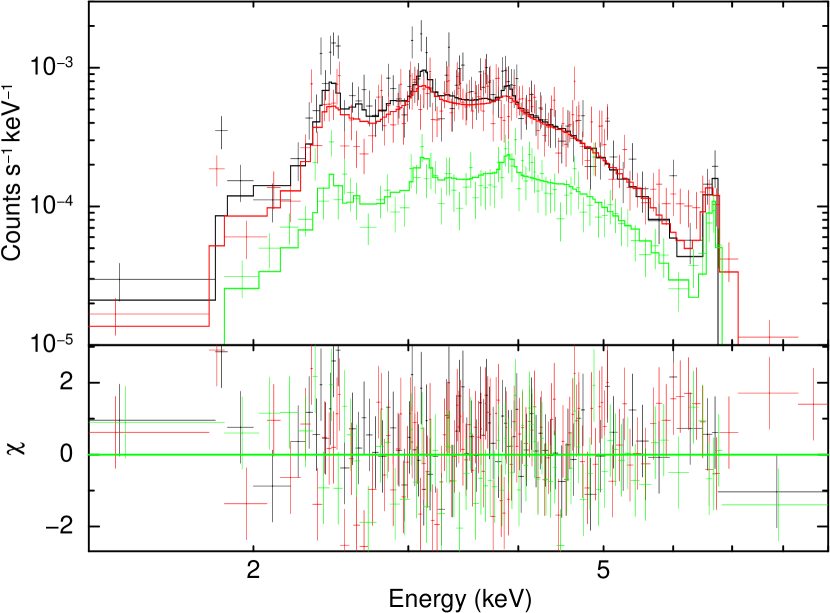
Figure 3: Chandra spectra of IRS 13E, together with the best-fit XSPEC VAPEC model (Table 2): ACIS-S/NONE (black) and ACIS-S/HETG 0th-order (green) and ACIS-I (red).

We examine how various modifications of the plasma model may affect the estimation of the spectral parameters. For example, one may expect that the ionization state of the plasma takes time to establish an equilibrium. We thus fit the spectra with the XSPEC VNEI model, even with separate grouping of metals into $\alpha$-elements and Fe-like elements. We find that this model does not significantly improve the fit to the spectra (e.g., $\chi^{2}/d.o.f.=$ 310/265). The modeling does give a probably meaningful constraint on the ionization parameter as $\tau=2.3(1.2-5.2)\times 10^{11}{\rm~{}s~{}cm^{-3}}$. But other model parameters are hardly changed, compared to those listed in Table 2.

We further consider the possibility that the metal abundance pattern of the X-ray-emitting plasma in IRS 13E could be substantially different from that of the ISM. The stellar wind from the WC star, in particular, is rich in Carbon, presumably due to the early triple-$\alpha$ nuclear synthesis and exposed now due to the mass loss. Although the X-ray emission lines of Carbon ions are too low energies to show up in the observed spectra of IRS 13E, because of the strong LoS X-ray absorption, the Bremsstrahlung continuum can be enhanced due to its proportionality to $Z^{2}$, where $Z$ is the charge of an ion. (It is easy to show that H and He nuclei have the same efficiency, per unit mass, for producing the Bremsstrahlung continuum.) This continuum enhancement due to the enrichment of a particular metal, if not specifically considered as in the above model fits, could in general lead to an underestimate of the metal abundance. For a WC star, we may assume that only the Carbon enrichment is important, while the abundances of other tracer metals (e.g., Fe) remain unchanged, compared to those in the ISM. The continuum enhancement factor is then $[Zf_{Z}/2+(1-f_{Z})]$, where $Z=6$ is the atomic number of Carbon (the factor of 2 arises from the ion mass $2Z$) and $f_{Z}$ is the mass fraction of the ion. Because $f_{Z}$ can be up to $\approx 0.5$ (Koesterke & Hamann 1995), this factor can reach to $\sim 2$. The resultant underestimate of the metal abundance can then be up to the same factor. In contrast, the Nitrogen enrichment of a WN star should have little effect on the Bremsstrahlung efficiency. This enrichment is due to the conversion of C and/or O to N in the CNO cycles of hydrogen burning. Thus the stellar wind of a WN star is primarily composed of Helium. Therefore, with a more realistic stellar wind contributions from the WC and WN stars in IRS 13E, the metal abundance underestimate should be quite modest. With this estimate in consideration, we conclude that our metal abundance listed in Table 2 is consistent with the previous measurements (Cunha et al., 2007; Davies et al., 2009; Wang et al., 2006; Capelli et al., 2012).

We estimate the mean electron density of the plasma in IRS 13E as $n_{e}\sim 6\times 10^{2}{\rm~{}cm^{-3}}$, based on the size of the diffuse X-ray emission region, as well as the normalization listed in Table 2 and its standard XSPEC definition. Together with the plasma temperature, this leads to an estimate of the pressure as $P/k\sim 2\times 10^{10}{\rm~{}K~{}cm^{-3}}$. The plasma is thus strongly over-pressured, compared to the general ISM in the GC  ($P_{ISM}/k\sim 10^{5}-10^{9}{\rm~{}K~{}cm^{-3}}$; e.g., Rathborne et al., 2014).

4 Constraints on X-ray emission from the putative IMBH

We check whether an IMBH in IRS 13E may contribute to the observed X-ray emission. In § 3.1, we have used the spatial decomposition of the observed X-ray emission to constrain the contribution from a potential central point-like source in IRS 13E. This source could represent the accretion of the stellar wind material by this putative IMBH. Our upper limit on the source luminosity, $L_{x}\sim 6\times 10^{32}{\rm~{}ergs~{}s^{-1}}$ in the 2-10 keV band (§ 3.1), is certainly far less than the Eddington limit of the IMBH, $L_{Edd}\sim 2\times 10^{42}M_{IMBH,4}{\rm~{}ergs~{}s^{-1}}$, where $M_{IMBH,4}$ is the IMBH mass in units of $10^{4}{\rm~{}M_{\odot}}$. The IMBH, if present, should then be undergoing a radiatively inefficient accretion, as in the case for Sgr A* (e.g.,  Wang et al. 2013).

Could such a radiatively inefficient IMBH explain the possible point-like component of the X-ray emission? In the hot accretion case, the spatial distributions of the plasma density and temperature of the accretion flow can be scaled with their values at the so-called Bondi radius $r_{b}\propto M_{IMBH}$ (e.g., Roberts et al., 2017). This radius characterizes the size of the region in which the plasma of certain thermal and/or kinematic properties can be initially captured by the gravity of the black hole. Although the Bondi accretion model itself is typically too simplistic to describe the complex accretion process, the X-ray emission from the hot gas accretion is qualitatively dominated by the outer accretion flow (e.g., Wang et al., 2013; Roberts et al., 2017). One may then expect that $L_{x}\propto r_{b}^{3}n_{e}^{2}\propto M^{3}_{IMBH}n_{e}^{2}$. Our estimated $n_{e}$ in IRS 13E is a factor of nearly 4 higher than the value at the Bondi radius of Sgr A* (Roberts et al., 2017). Since Sgr A* is $L_{x}\approx 3.4\times 10^{33}{\rm~{}ergs~{}s^{-1}}$, the luminosity of the accreting IMBH should then be $\sim 9\times 10^{26}M^{3}_{IMBH,4}{\rm~{}ergs~{}s^{-1}}$, far too weak to explain the X-ray emission of IRS 13E.

The IMBH might, however, be located very close to one of the WR stars, and be accreting from its freely expanding stellar wind. In this case, the wind density decreases with the distance $r$ from the star. Our upper limit to the point-source luminosity, for example, would be reached if $r\lower 2.0pt\hbox{$\,\buildrel\scriptstyle<\over{\scriptstyle\sim}\,$}6\times 10^{-4}{\rm~{}pc}~{}\dot{M}_{w,-5}^{1/2}v_{w,3}^{-1/2}$, where $\dot{M}_{w,-5}$ and $v_{w,3}$ are the mass-loss rate and stellar wind speed in units of $10^{-5}{\rm~{}M_{\odot}~{}yr^{-1}}$ and $10^{3}{\rm~{}km~{}s^{-1}}$, respectively. This distance corresponds to $\lower 2.0pt\hbox{$\,\buildrel\scriptstyle<\over{\scriptstyle\sim}\,$}0.1^{\prime\prime}$ in projection, which means that the X-ray source should spatially almost coincide with one of the WR stars, which is inconsistent with our measurement of the X-ray peak centroid (§ 3). Therefore, the putative IMBH, accreting from the stellar wind material, is not expected to contribute significantly to the observed X-ray emission.

5 Hydrodynamic simulations and comparison with the X-ray observation

The spatial and spectral properties of IRS 13E strongly suggest that its X-ray emission arises primarily from the CW in the group (Coker et al., 2002). In this scenario, the stellar winds are heated in standing shocks around the stars. The characteristic temperature of the shock-heated gas is $1.5\times 10^{7}v_{w,3}^{2}$ K, roughly consistent with the measured value in IRS 13E (Table 2). At least part of the X-ray emission from IRS 13E must originate in the CW. The mechanical energy input rate from the stars is $L_{{IRS~{}13E}}\sim(3\times 10^{37}{\rm~{}ergs~{}s^{-1}})\dot{M}_{-4}v^{2}_{w,3}$. Only $\sim 10^{-4}$ of this wind energy input is required to produce the X-ray luminosity of IRS 13E. The rest of the energy must be carried out by the combined group wind, escaping into a larger region and regulating the environment of the Galactic nucleus (e.g., Calderón et al., 2019b).

Here we attempt to check the consistency of the CW scenario with the above observational results more quantitatively, via simulations. We first update hydrodynamic simulations of the central parsec around Sgr A* that include IRS 13E and then compare synthesized spectra and images with the observed ones. This part of our study follows the same method of Russell et al. (2017), the relevant details of which we recap here.

With the purpose of studying the gas dynamics around Sgr A*, Cuadra et al. (2008, 2015) performed smoothed particle hydrodynamic simulations of the central 25 WR stars and their stellar winds within 1 pc of the SMBH. Using the location of the stars 1100 yr ago as the initial condition, the simulations had the stars orbit the SMBH while ejecting gas particles to model their stellar winds up to a few hundred years into the future. The construction of the orbits used the existing 3-D velocity measurements of individual stars and their positions on the sky, as well as their assumed orbit shape (quasi-circular or following the so-called clockwise disk (Paumard et al., 2006)), which constrain their unknown LoS locations. But this constraint can be rather uncertain for specific objects such as stars in the IRS 13E group. The orbits of individual stars within the group are also unknown, depending largely on its assumed total mass. The Cuadra et al. simulations included an IMBH of 350 M_⊙ in between the stars of the group (Fritz et al., 2010). The winds from the 25 WRs naturally collide with one another, creating a complex, time-varying reservoir of shock-heated gas, a small fraction of which is captured by Sgr A*.

The hydrodynamic simulations, confronted with Chandra observations, can be used to test the CW scenario, and to constrain the relative line-of-sight position and the wind properties of the stars. Russell et al. (2017) synthesized the spatially resolved thermal X-ray emission from the simulations by using the optically-thin plasma VVAPEC model for the emission, which was split into three abundance-specific spectral classes: WC, early WN, and late WN. The resulting pixel-by-pixel spectra were folded through the instrument response function, and then 4-9 keV images and 2″-5″annulus spectra were extracted to compare directly with the observations. The best-matched model, which incorporated feedback from the SMBH to clear out some of the hot gas from the region surrounding Sgr A* (Cuadra et al., 2015), agreed in the image and spectra to within  20%. However, the IRS 13E group was not well matched; the synthesized X-ray emission is greater than the observed flux, regardless of Sgr A* feedback model, indicating either that the stars were too close in 3D separation and/or that the wind parameters used, i.e. mass-loss rates and/or wind speeds, were too high (see below).

We conduct multiple simulations tuned to match the Chandra data of IRS 13E. Its X-ray spectral shape in the adiabatic CW scenario considered here depends primarily on the stellar wind speeds of individual stars, chiefly E2 and E4, but also on their relative mass-loss rates. The spatial extent of the X-ray emission scales linearly with the separation between two stars ($\delta D$), which cannot be directly observed and could be much greater than what is assumed in the simulation (roughly the projected distance of $\sim 0\aas@@fstack{\prime\prime}3$). The luminosity of the emission scales with the combined mass-loss rate of the two stars ($\dot{M}_{w}$), as well as $\delta D$, according to

$$L_{x}\propto\dot{M}_{w}^{2}/\delta D.$$ (1)

Our simulations sample various stellar wind speed and mass-loss rate ratios, around the predictions from the stellar types of the stars (Russell et al., 2017, and references therein), while the remaining 23 WR stars in the simulations are unchanged. From the comparison of the simulated X-ray spectra and sizes with the observed ones of IRS 13E, we constrain $\delta D$, as well as the stellar wind speeds and mass-loss rates of the stars.

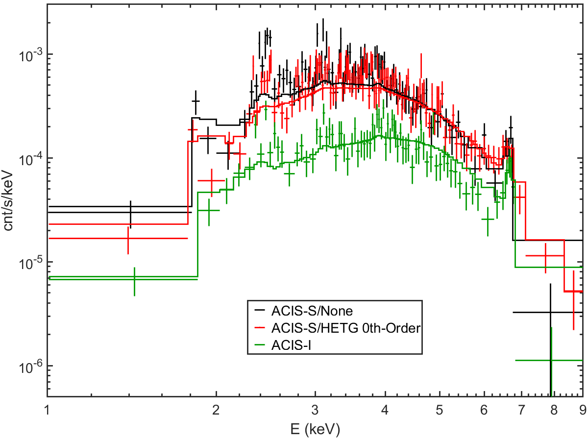
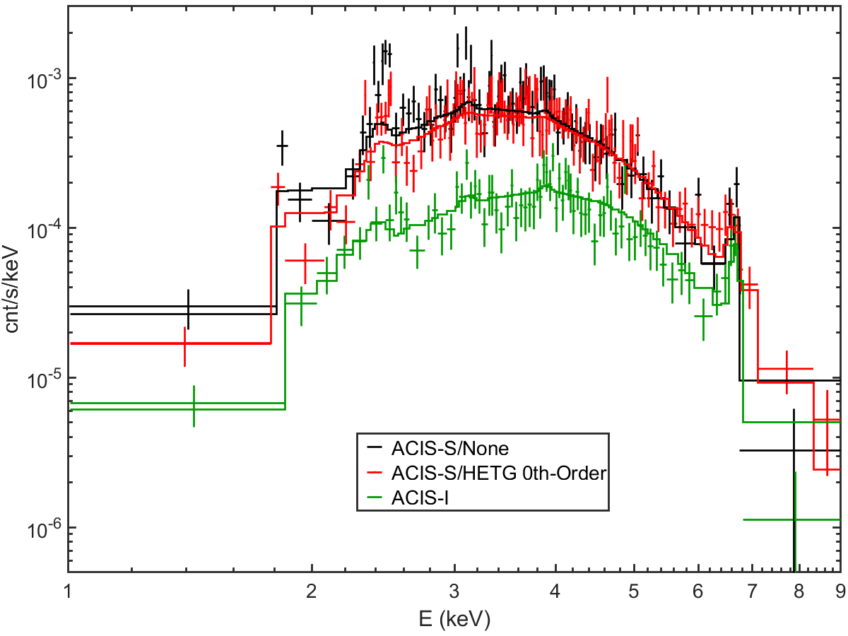
Figure 4: Representative fits of simulated model spectra to the same Chandra data as in Fig. 3: our initial ”best guessed” model (upper panel) and the ”best fit” model (lower panel) with the parameters listed in Table 3.

For the new set of simulations run for this work, we start with a ”best guessed” set of stellar wind parameters for the two WR stars in IRS 13E. We reduce the WC wind as its analysis was subject to significant dust contamination, which might be the reason for its wind speed and mass-loss rate apparently being larger than the other WC stars in the GC (Martins et al., 2007). For the WN wind, updated modeling of the mass-loss rate in other GC WN stars reduces the mass-loss rate by a factor of $\sim$2 (Yusef-Zadeh et al., 2015). The reduction factors of 2 for both $\dot{M}$ and 1.5 for the WC wind speed provides our initial ”best guessed” model presented in Table 3. In the subsequent runs, we adjust the parameters one by one, not only to bring the model into better agreement with the model, but also to verify expected trends in how the X-ray emission is sensitive to the wind speeds and the wind momentum ratio.

To have as detailed a model-to-observation comparison as possible, we process the model images and spectra in the same manners as for the observations. Specifically, the spectral fits are performed in an analogous method to the VVAPEC fitting of the observed data, namely using xspec to simultaneously fit all three Chandra spectra where the hydrodynamic+emission model spectra, extracted in the same projected regions, are absorbed by the ISM according to the tbabs model with wilms abundances. This absorption is fixed at the best-fit ${\rm N_{H}}$ (Table 2) to reduce the number of variables for the present modeling.

Table 3: Model parameters of the IRS 13E WR stars

Parameter	Value
	“best guessed”	“best fitted”	‘normalized best fitted”
E2 (WC) $\dot{M}$	$2.5\times 10^{-5}{\rm~{}M_{\odot}~{}yr^{-1}}$	$3.3\times 10^{-5}{\rm~{}M_{\odot}~{}yr^{-1}}$	$6.3\times 10^{-5}{\rm~{}M_{\odot}~{}yr^{-1}}$
E2 (WC) $v_{w}$	1500 ${\rm~{}km~{}s^{-1}}$	750 ${\rm~{}km~{}s^{-1}}$	750 ${\rm~{}km~{}s^{-1}}$
E4 (WN) $\dot{M}$	$2.2\times 10^{-5}{\rm~{}M_{\odot}~{}yr^{-1}}$	$2.9\times 10^{-5}{\rm~{}M_{\odot}~{}yr^{-1}}$	$5.5\times 10^{-5}{\rm~{}M_{\odot}~{}yr^{-1}}$
E4 (WN) $v_{w}$	750 ${\rm~{}km~{}s^{-1}}$	750 ${\rm~{}km~{}s^{-1}}$	750 ${\rm~{}km~{}s^{-1}}$
$\delta D$	0.013 pc ($\equiv 0\aas@@fstack{\prime\prime}34$)	0.014 ($\equiv 0\aas@@fstack{\prime\prime}34$)	0.05 pc ($\equiv 1\aas@@fstack{\prime\prime}3$)

Note: The initial $\dot{M}$ values for the ”best guessed” model given here are not adjusted for a small normalization correction that gives the fit to the Chandra spectra shown in Fig. 4 upper panel. The ”best fit” model gives an optimal fit to the observed Chandra spectra (Fig. 4 lower panel). The ”normalized best fit” model is the same as the ”best fit” mode in terms of the spectral fit; but the listed $\dot{M}$ values are normalized according to Eq. 1 from $\delta D=0.014$ pc (used in the ”best fit” model simulation) to $\delta D=0.05$ pc, which gives a spatially scaled radial intensity profile that reasonably well matches the Chandra data (Fig. 5B).

Fig. 4 illustrates the results of the simulated spectral fits to the observed data. The initial ”best guessed” model produces a too flat spectrum (due to the still relatively high wind speed assumed) to fit the observed data well, evident at energies $\lower 2.0pt\hbox{$\,\buildrel\scriptstyle>\over{\scriptstyle\sim}\,$}4.5$ keV. Although the ”best fit” model fits the data reasonably well (with a reduced $\chi^{2}=1.32$), it indicates that the E2 wind speed needs to be cut further in half, compared to the ”best guessed” model (Table 2). Such a low speed value of the WC stellar wind seems to be a bit extreme, in reference to its canonical value. Furthermore, we have here used the X-ray absorbing ${\rm N_{H}}$ as inferred from the best fit of the VVAPEC model to the Chandra spectra. As discussed in § 3.2, the real ${\rm N_{H}}$ could be 30% higher. With this higher ${\rm N_{H}}$, the model spectrum would need to be even softer (i.e., demanding even a lower wind speed) to match the observed ones.

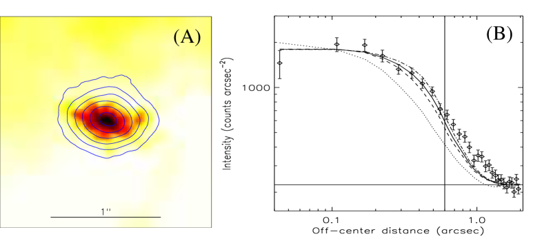
Figure 5: (A) Close-up image of the 1-9 keV intensity of IRS 13E, constructed from the “best fit” model simulations assuming $\delta D=1\aas@@fstack{\prime\prime}3$, shown in a logarithmic scale. The overlaid illustrative intensity contours are obtained from the same image after being convolved with the PSF of the Chandra observation (see the text). (B) Comparison of the radial model intensity profiles of the PSF-convolved image (solid) with the Chandra profile in the 1-9 keV band (data points), as presented in Fig. 2A. The vertical line at $r=0\aas@@fstack{\prime\prime}6$ indicates the projected radius or the off-center distance within which the model profile matches the Chandra profile well. The horizontal line marks the background level estimated with the Chandra data in the 1$\aas@@fstack{\prime\prime}$5 and 2″ range. We have added this level to the model profile after both subtracting its background estimated in the same range and scaling the mean flux of the first three data to the corresponding Chandra value. For comparison, similarly constructed model profiles in the 1-4 keV (dashed) and 4-9 keV (dash-dotted) bands, as well as in the 1-9 keV band but assuming $\delta=0\aas@@fstack{\prime\prime}3$ (dotted) , are also shown.

In addition to the spectra, the X-ray synthesis also produces images. Fig. 5A shows the 1-9 keV emission centered on IRS 13E for the ”best fit” model before and after PSF folding. The pre-PSF image is clearly aspherical; the minor axis of the asymmetry is along the line of the two WR stars, so the major axis with a position angle $\approx 80^{\circ}$ east to the north traces the dominant shocked gas and hence the X-ray emission, closer to E2 than E4, as determined by the ram-pressure balance between the stellar winds. After folding the X-ray models through a Chandra PSF, the aspherical nature of the emission is naturally reduced, depending on the assumed $\delta D$.

The morphology as indicated by the contours shown in Fig. 5A for our chosen $\delta D\sim 1\aas@@fstack{\prime\prime}3$ (compared to $\delta D=0.014$ pc used in our simulation) resembles that of the emission from the inner region of IRS 13E in the Chandra image (i.e., the region enclosed by the 3rd contour in Fig. 1A). This similarity is also seen in the radial intensity profile comparison within $r\lower 2.0pt\hbox{$\,\buildrel\scriptstyle<\over{\scriptstyle\sim}\,$}0\aas@@fstack{\prime\prime}6$, where a good match to the Chandra profile is found for the synthesized one when it is scaled up to $\delta D\sim 1\aas@@fstack{\prime\prime}3$, which is a factor of $\sim 4$ larger than the projected separation between E2 and E4 (Fig. 5B). Outside this radius, the model systematically under-predicts the intensity. The predicted profile in the 4-9 keV band is only slightly broader than than in the 1-4 keV band. The model profiles are all substantially steeper than the observed one. The intensity excess above the best-matched model here is about 28% of the total observed flux in the 0$\aas@@fstack{\prime\prime}$6-1$\aas@@fstack{\prime\prime}$5 range, but accounts of only about 10% of the flux within the 1$\aas@@fstack{\prime\prime}$5 radius. The CW seems to dominate the overall observed emission and the required mass-loss rates of the two WR stars are quite high (Table 3). This result seems to be quite robust, insensitive to the stellar wind parameter choice.

With the change of $\delta D$ from 0$\aas@@fstack{\prime\prime}$34 (used in the simulation) to 1$\aas@@fstack{\prime\prime}$3, which better matches the observed radial intensity profile, we infer from Eq. 1 the corresponding $\dot{M}$ values, assuming the same X-ray luminosity (or the spectral normalization) that gives the ”best fit” to the Chandra spectra. These inferred $\dot{M}$ values are listed under the ”normalized best fit” model in Table 2.

However, the above $\delta D$ scaling represents an upper limit to the extent that the CW X-ray emission extends. $\delta D$ could be significantly smaller than $1\aas@@fstack{\prime\prime}3$. If this is the case, then even a larger fraction of the observed extended emission needs to be explained with a contribution in addition to the CW (see § 8 for further discussion).

There are a few other more subtle observed characteristics that are not well accounted for by the simple CW scenario. These features include the apparent offset of the X-ray centroid to the west of the two WR stars and the fan-out morphology of the X-ray emission toward the SE (§ 3.1), as well as the softness of the observed X-ray spectra, compared to the simulated ones. We hypothesize that these characteristics, as well as the observed excess emission in the 0$\aas@@fstack{\prime\prime}$6-1$\aas@@fstack{\prime\prime}$5 range, are due to an additional X-ray contribution from the interaction of the IRS 13E cluster wind with its ambient medium. We explore this idea below, together with other lines of observational evidence for the interaction.

6 ALMA observations of IRS 13E

6.1 Description of ALMA observations and data processing

ALMA observations allow us to sensitively probe cool gas in the GC, as has been demonstrated in several publications (e.g., Moser et al., 2017; Tsuboi et al., 2016, 2017a, 2017b, 2019; Murchikova et al., 2019). Our study here is meant to complement published results and to provide new insights into the spatial and kinematic properties of the gas. While our analysis of relevant observations will be detailed in a separate paper on broader issues of the GC (Li et al.  2019 in preparation), the present study primarily uses the ALMA band-6 observation taken in May and July, 2017 for the project 2016.1.0087.S, which is focused on the accretion flow toward Sgr A* (PI: Elena Murchikova). When we started this part of the study, this observation gave us the highest spatial resolution view of the H30$\alpha$ hydrogen recombination line emission of IRS 13E. No existing publication has used this observation – Murchikova et al. (2019) actually used earlier observations. Our focus here is of course on IRS 13E.

We use the Common Astronomy Software Applications package (CASA) version 5.1.1 for standard data processing. The achieved synthesized beam of the observation is $0\aas@@fstack{\prime\prime}22\times 0\aas@@fstack{\prime\prime}13$ (FWHM). We apply the primary beam correction for all the ALMA images presented in the present work. The final H30$\alpha$ data cube has a spectral resolution of $22~{}{\rm~{}km~{}s^{-1}}$ and a channel noise of $\sigma_{\rm ch}\approx 0.08{\rm~{}mJy~{}beam^{-1}}$, estimated with line-free channels and regions. The moment zero intensity of the H30$\alpha$ line emission, integrated from velocity from $-400~{}{\rm~{}km~{}s^{-1}}$ to $400{\rm~{}km~{}s^{-1}}$, has a noise of $\sigma_{\rm mom.0}\approx 0.04{\rm~{}Jy~{}beam^{-1}km~{}s^{-1}}$, while the continuum emission has $\sigma_{\rm cont}\approx 0.1{\rm~{}mJy~{}beam^{-1}}$.

6.2 ALMA results

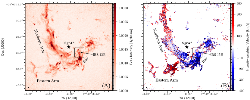
Figure 6: An ALMA overview of the GC field: (A) the H30$\alpha$ line peak emission map; (B) the intensity-weighted velocity map. Major ionized gas streams or arms of the minispiral, together with key objects relevant to the present study, are labeled. The small rectangular box marks the IRS 13E close-up region shown in Fig. 7.

Fig. 6 presents an ALMA overview of the GC field, covering all the major relevant objects and features discussed in the present study, while Figs. 7 and 8A give close-ups of IRS 13E and its immediate vicinity. Fig. 8A further demonstrates a good correspondence of ALMA emission peaks with compact radio sources (Zhao et al., 2009). These plots show that IRS 13E is an outstanding millimeter (mm) wave-emitting source, particularly in terms of the H30$\alpha$  emission. Both the mm continuum and the line emission are centrally peaked with their centroids consistent with each other, located between E2 and E4 (Fig. 7; the two WRs only show weak 232 GHz continuum emission, but no significant H30a emission in the higher resolution image of Tsuboi et al. 2019). This central peak, identified as the near-IR dust emission complex E3 (e.g., Fritz et al., 2010; Tsuboi et al., 2019), is rather compact, but still clearly resolved. In addition to the strongly peaked line and continuum emission, interesting surrounding structures are apparent in the plots. We detail the morphological and kinematic properties of these features in the following.

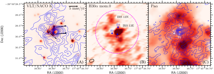
Figure 7: Close-up views of IRS 13E and its immediate surrounding: (A) the ALMA integrated intensity contours of the 232 GHz continuum overlaid on a VLT/NACO K-band image, together with proper motion vectors of IR sources (Fritz et al., 2010); (B) H30$\alpha$ line integrated emission intensity map; (C) H30$\alpha$ intensity contours compared with the diffuse Pa-$\alpha$ line emission image (Wang et al., 2010; Dong et al., 2011). The beam size is illustrated in the lower-left corner of Panel B. While the VLT IR image in (A) was taken in 2005, 12 years earlier than the ALMA observation, the positions of E1, E2, and E4 marked with the plus symbols in all three panels have been corrected for the proper motions ($\sim 0\aas@@fstack{\prime\prime}08$) (Paumard et al., 2006). The magenta circle in (B) outlines a region of 1^′′ radius around E3, from which the H30$\alpha$  flux is extracted in § 8.5.

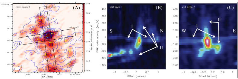
Figure 8: (A) Close-up of IRS 13E and its immediate vicinity in the ALMA 232 GHz continuum (contours) and H30$\alpha$ line (image) emissions. Compact radio sources taken from Zhao et al. (2009), as well as other key stellar objects in IRS 13E, are also marked with yellow solid dots and plus signs respectively. The two rectangular cut areas (1 and 2) mark the regions through which the position-velocity diagrams, as shown in panels (B) and (C), respectively, are extracted. In these latter panels, the two velocity components (I and II), as well as the directions (S and N, E and W) of the cuts, are marked.

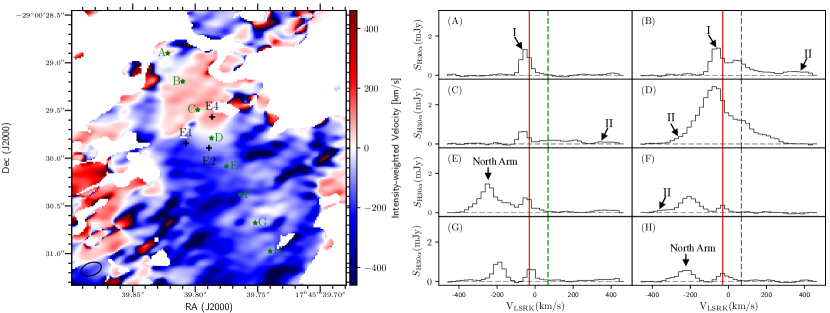
Figure 9: H30$\alpha$ intensity-weighted velocity map (left panel) and line profiles (right Panels A-H) extracted from the locations marked with the stars along the NE-SW oriented straight line in the left panel. All the line profiles are obtained within a beam-sized aperture. The solid and dashed vertical lines mark the LoS velocities of the bar and IRS 13E, as listed in Table 1. The two velocity components (I and II), in addition to the Northern Arm, are marked.

We confirm the presence of H30$\alpha$-emitting gas with a very large LoS velocity spread (Tsuboi et al., 2017b, 2019). While Appendix A presents the channel maps of the H30$\alpha$ emission, Figs. 8 B and C present the position-velocity diagrams in two particular directions across IRS 13E. Fig. 9 shows the mean LoS velocity structure resolved on scales down to $\sim$ 1600 AU. Gas on the immediate northeastern (NE) side of E3 is primarily redshifted, reaching $\sim+100{\rm~{}km~{}s^{-1}}$ on average, whereas the blueshifted gas as much as $\sim-200{\rm~{}km~{}s^{-1}}$ is on the opposite side. Gas with even higher negative velocities appears mostly in regions further south ($\lower 2.0pt\hbox{$\,\buildrel\scriptstyle>\over{\scriptstyle\sim}\,$}1\arcsec$ away from E3) and is apparently connected to the large-scale components D and C with velocities $\sim-340~{}{\rm~{}km~{}s^{-1}}$, as identified by Tsuboi et al. (2017b). This can also be appreciated in Figs. 8B and C.

From examining the position-velocity diagrams and the H30$\alpha$ line profiles across the region (e.g., Figs. 8 and 9), we can further determine the LoS velocity distribution of the H30$\alpha$ emission. We identify two interesting LoS velocity components. Component I is relatively narrow and centered at $\sim-30{\rm~{}km~{}s^{-1}}$. It most probably corresponds to the bar of the minispiral (Table 1). This narrow bar component seems to be present across the IRS 13E  region in Fig. 9, although confusion with other components is considerable at various locations. The significance of the component in general decreases from the NE to SW. At the location of IRS 13E (see Panel D), the bar component is greatly enhanced in both intensity and LoS velocity spread.

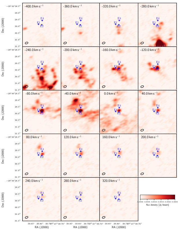
Figure 11: ALMA channel maps of the H30$\alpha$ line emission in the IRS 13E region, from $-400{\rm~{}km~{}s^{-1}}$ to $320{\rm~{}km~{}s^{-1}}$ and with the velocity bin size of $40{\rm~{}km~{}s^{-1}}$. The average root mean square in line-free channels is about 0.07 mJy beam^-1. The positions of E1, E2 and E4 are marked for ease of reference.

Component II is very broad (with a total spread of $\sim 800{\rm~{}km~{}s^{-1}}$) and is centered roughly at $\sim+44{\rm~{}km~{}s^{-1}}$ – the systemic velocity of IRS 13E (Table 1). This component is seen within about 1″ of IRS 13E and is in general quite faint ($S_{H30\alpha}\lower 2.0pt\hbox{$\,\buildrel\scriptstyle<\over{\scriptstyle\sim}\,$}0.2$ mJy; Figs. 9 and 8), except for at the center of the group. On the NE side of the group, the component is seen essentially only on the redshift side, up to $\sim+420{\rm~{}km~{}s^{-1}}$ (Panels B-C). But starting at IRS 13E (Panel D) and toward the SW, extended blueshifted emission (probably reaching $\sim-320{\rm~{}km~{}s^{-1}}$) appears, although the velocity spread is very much confused with a distinctly narrow feature, which peaks at $\sim-220{\rm~{}km~{}s^{-1}}$ (Panels E and F) and represents the continuation of a large-scale coherent structure toward the south, as part of the North Arm (Fig. 6B). We do not analyze this feature further in this work. Nevertheless, Component II is still visible at velocities $\sim-300{\rm~{}km~{}s^{-1}}$ to $-400{\rm~{}km~{}s^{-1}}$, especially in Panel F (see also Fig. 8B). Probably because the H30$\alpha$-emitting gas is quite lumpy and/or the sensitivity of the data is too limited (see § 8.4 for discussion), the component is not apparent in the 2-D channel maps (Fig.  11). Thus its global structure remains uncertain.

Components I and II probably reflect the influence of IRS 13E on the ambient gas in two different regions. Component I is very local to the central region of IRS 13E, between E2 and E4, whereas Components II is over a relatively larger scale up to $\sim 1^{\prime\prime}$ radius.

7 Critical examination of existing results and interpretations

Tsuboi et al. (2019) have recently reported a very high-resolution ALMA observation of IRS 13E (beam size $0\aas@@fstack{\prime\prime}037\times 0\aas@@fstack{\prime\prime}024$). This observation allows them to resolve the central thermal emission peak into multiple features, including extended ones in both the continuum and H30$\alpha$ emissions. The reported work is focused on the brightest extended feature E3, which is characterized with a 2-D Gaussian of sizes $=0\aas@@fstack{\prime\prime}093\times 0\aas@@fstack{\prime\prime}061$. They estimate the density and thermal pressure of the region as $n_{e}=6\times 10^{5}{\rm~{}cm^{-3}}$ and $P/k\sim 8\times 10^{9}{\rm~{}K~{}cm^{-3}}$. Interestingly, this thermal warm gas pressure is comparable to that inferred for hot gas in IRS 13E (§ 3.2), indicating that two gas phases are in rough pressure balance.

The H30$\alpha$ emission shows a large velocity gradient, ranging from $\sim-180{\rm~{}km~{}s^{-1}}$ (at the SE) to $\sim 150{\rm~{}km~{}s^{-1}}$ (NW). This velocity gradient is nearly opposite to that on larger scales (§ 6.2). Tsuboi et al. (2019) interpret E3 as a ring-like structure rotating around a dark object and having an inclination angle of $i\sim 50^{\circ}$. The inferred mass of this object is $2.4\times 10^{4}M_{\sun}$, which could then be the putative IMBH. The structure, however, has to be highly asymmetric or lopsided in its brightness distribution (see Fig. 4a in Tsuboi et al. 2019). The NE part of the structure is substantially brighter than the SW.

The position and structure of E3 vary with time. A comparison of the ALMA data with a VLA radio image, taken in 1990s and with resolution of $0\aas@@fstack{\prime\prime}09\times 0\aas@@fstack{\prime\prime}06$, shows an apparent change in the orientation of the emission morphology of E3, which is called HII-7E in Zhao & Goss (1998). The radio image shows a NW-SE orientation (see Fig. 4 in Zhao & Goss, 1998), which is nearly perpendicular to that seen in the ALMA observation (Tsuboi et al., 2019). This systematic orientation change is at least qualitatively consistent with the differential proper motions (predominately in the Declination direction) between the NW and SE parts, labeled as IRS 13W and IRS 13E in Zhao & Goss (1998). This work also finds little proper motion of E3 in the RA direction, in sharp contrast to E2 and E4, which show large westward motion (Table 1; see also Fig. 5 in Eckart et al. 2013). This difference explains the changing position of E3 relative to E2 and E4, from the west side (in 1990s) to the east side (in 2018; Tsuboi et al. 2019).

Variability is also seen in the comparison of the ALMA data with a co-add of near-IR images taken between 2002 and 2007 (see Fig. 1 in Fritz et al. 2010). In this co-add, E3 can be decomposed into six clumps (E3.0-3.5). The overall morphology of the near-IR E3 emission (e.g., the east-west elongation) is similar to that seen in the ALMA image (e.g., Fig. 4a; Tsuboi et al. 2019). However, E3 is evidently brighter on its western part (peaking at E3.0) in the co-add, whereas the NE part is enhanced in the ALMA image (see Fig. 4a;  Tsuboi et al. 2019). Furthermore, the LoS velocity of E3.0 – the peak of the E3 complex – has changed from $\sim-25{\rm~{}km~{}s^{-1}}$ (Fritz et al., 2010) to $\sim-75{\rm~{}km~{}s^{-1}}$ (Tsuboi et al., 2019). Such drastic variations have taken place on a time interval of $\sim 15$ yr between the near-IR and ALMA observations, for example, which may be allowed by the orbital motion with a period of 50-100 yr in the IMBH interpretation (Tsuboi et al., 2019).

However, there might be some difficulties in the IMBH interpretation of E3. First, for a ring around the IMBH, which dominates the gravitational mass of IRS 13E, one would expect an overall velocity spread symmetry relative to the group. The measured LoS H30$\alpha$ velocity spread of E3, as described above, is centered at $\sim-15{\rm~{}km~{}s^{-1}}$ (see also Fig. 4 in Tsuboi et al. 2019), apparently inconsistent with those of the three stars in IRS 13E (all have positive velocities; Table 1). Because they are located quite some distances away even in projection and on different sides of the putative IMBH, their velocities are not expected to drastically and systemically change over the last 15 years or so. Second, the proper motion pattern of the dusty clumps in E3 shows no indication of rotation (Fritz et al., 2010). Third, the proposal for the presence of the IMBH in IRS 13E is questioned based on measurements of stellar kinematics (Fritz et al., 2010). The mass constraint on the IMBH is largely based on upper limits on the expected reflex motion of Sgr A*, as well as the acceleration of E1 and the velocity differences between E1, E2, and E4. The constraint is greatly weakened if E1 is not bound to IRS 13E. In fact, the velocity vector of E1 is quite different from those of E2 and E4 with an offset of $\sim 174{\rm~{}km~{}s^{-1}}$ (Table 1). On the other hand, E2, and E4 are most likely bound. The probability for a chance coincidence of these two rare extreme objects to be so close in the phase space is extremely small, especially if they are at the distance of $\sim 10\arcsec$ off Sgr A* (see below and § 8). So we conclude that E2 and E4 are most likely bound, whereas E1 is not a member of the IRS 13E group.

Finally, the gravitational bounding between E2 and E4 requires that their separation $\delta D<2r_{J}$, where

$$r_{J}\sim D[m_{g}/(2M_{SgrA*})]^{1/3}$$ (2)

is the Jacobi radius of IRS 13E of a mass $m_{g}$ against the gravitational tidal force of Sgr A*. For the Sgr A* mass $M_{SgrA*}=4\times 10^{6}~{}M_{\sun}$, the orbital distance of the group from Sgr A* $D>7\arcsec\ (\delta D/1\aas@@fstack{\prime\prime}3)(m_{g}/10^{4}~{}M_{\sun})^{-1/3}$. This distance constraint is consistent with the hypothesis that IRS 13E is embedded within the mini-spiral bar, which is distributed within an orbital distance range of 7″ -20″ (Liszt, 2003, see also § 8). The constraint may also be compared with the group’s distance of $\sim 7\arcsec\ (V_{E2+4}/249{\rm~{}km~{}s^{-1}})^{-2}$ (Table 1) for a circular motion; a larger distance is allowed for an eccentric orbit. These arguments seem to favor the presence of an IMBH of mass $\sim 10^{4}~{}M_{\sun}$. However, such an IMBH is not necessary. With the group’s total stellar mass up to $\sim 2000~{}M_{\sun}$ (Fritz et al., 2010), for example, IRS 13E needs only be $D\lower 2.0pt\hbox{$\,\buildrel\scriptstyle>\over{\scriptstyle\sim}\,$}10\arcsec(\delta D/1\aas@@fstack{\prime\prime}3)$ away from Sgr A* to avoid tidal disruption. $\delta D$ could also be considerably smaller than our assumed 1$\aas@@fstack{\prime\prime}$3 here (see § 8).

In summary, the presence of the IMBH in IRS 13E helps to explain its gravitational bounding but has difficulties with the extreme gas kinematics. In the next section, we propose an alternative scenario for the gas kinematics.

8 Collision of IRS 13E with ambient dense gas

Energetic stellar winds in IRS 13E  not only collide with each other, but also unavoidably interact with its surrounding. The impact of this interaction depends on the density of the ambient medium, as well as the relative velocity between the group and the medium. We start by considering their kinematics and will then examine how the collision may explain the thermal emission features with unusually large velocity spreads, as well as various other outstanding phenomena in and around the group.

8.1 Kinematics of IRS 13E and its surrounding medium

Table 1 presents a summary of key velocity measurements relevant to the collision of the stellar winds from IRS 13E  with the surrounding gas. We first estimate the effective mean velocity of IRS 13E ($v_{E2+4}$) by averaging those measured for E2 and E4, which dominate the stellar wind energetics in the group. The result is included in Table 1.

Can $v_{E2+4}$ be considered as a representative velocity of IRS 13E? The answer depends on whether or not the internal velocity dispersion in the group, $\delta V\sim(2Gm_{g}/r_{e})^{1/2}$, is substantially smaller than the orbital velocity around Sgr A*, $V_{o}\sim(2GM_{SgrA*}/D)^{1/2}$. Using Eq. 2 and assuming that the effective radius of the group ($r_{e}$) is comparable to $r_{J}$, we can approximately express the ratio as

$$\delta V/V_{o}\sim 2^{1/6}(m_{g}/M_{SgrA*})^{1/3}=0.15(m_{g}/10^{4}~{}M_{\sun})^{1/3}.$$ (3)

Therefore, we may reasonably use $v_{E2+4}$ as the systematic velocity of IRS 13E.

We next consider the velocity of the minispiral bar. We have shown in § 6 that the H30$\alpha$ emission of E3 peaks around the LoS velocity of the bar, which we assume is due to the collision. To figure out what direction the collision is in, we need to know the relative transverse motion between IRS 13E and the bar. To do so, we use proper motion measurements of various thermal gas blobs in and around IRS 13E (e.g., Zhao et al., 2009). These measurements, made with high-resolution VLA observations, show that proper motion vectors point in many different directions, which may be largely due to the dispersing of the blobs by the stellar winds. We average the vectors to estimate the undisturbed motion of the bar. We find that the averaged vector is primarily toward the west with a speed of $v_{\rm RA}\sim-150{\rm~{}km~{}s^{-1}}$. In the Declination direction, however, the averaged vector is short, varies from one work to another and can be positive or negative (e.g., Zhao & Goss, 1999; Zhao et al., 2009). Therefore, we approximate $v_{\rm Decl.}\sim 0{\rm~{}km~{}s^{-1}}$ for the bar in Table 1.

Recent studies suggest that the bar is a distinct gaseous structure orbiting around Sgr A*. Liszt (2003) shows that the bar can be reasonably well represented by a kinematic model of a series of thin co-planar rings rotating at the local circular velocity around Sgr A*. This set of rings is assumed to extend from 0.3 to 0.5 pc in radius and to be nearly edge-on and perpendicular to the Galactic plane. Tsuboi et al. (2017a) favor this near-polar ring interpretation, but suggest that the orbits of the rings may be highly eccentric. In both models, the bar at the location of IRS 13E  is largely moving from the east to the west and just changes the LoS component from redshift to blueshift. Within their large uncertainties, the model predictions are consistent with the velocities that we have adopted for the bar at IRS 13E.

8.2 Scenario for the collision between IRS 13E and its ambient gas

With the estimates of the relative motion between IRS 13E and the bar, we can now check what kind of collision they may be experiencing and what it could produce. With a speed of $\sim 1.4\times 10^{2}{\rm~{}km~{}s^{-1}}$ (Table 1), this collision should be supersonic. We thus expect that a bow shock forms around IRS 13E, as illustrated in Fig. 10. The morphology of this bow shock depends on the exact 3-D locations of the stars, especially those (E2 and E4) with strong stellar winds, and their energetics, as well as the direction of the collision, all of which are quite uncertain. Nevertheless, with our rough estimates of the velocity vector of the relative motion ($v_{\rm RA},v_{\rm Decl.},v_{z}=-88,-39,+98{\rm~{}km~{}s^{-1}}$; Table 1), the collision seems mostly along the LoS direction and toward the west (slightly to the south). The high-speed collision, together with the strong ionizing radiation and stellar winds of the group, should also produce an energetic champagne flow in the opposite direction of the relative motion.

We have examined existing works to explore the characteristics of the bow shock and champagne flow. There are various models that incorporate the effect of ionizing radiation and stellar winds. Such models have been explored in 2-D simulations (Arthur & Hoare, 2006), which show limb-brightened morphology of warm gas, instabilities in the swept-up shell with density fluctuations, and champagne flows with complicated kinematics. However, the collision between IRS 13E and the bar is far more extreme than what are assumed in the existing modeling, in terms of the relative velocity and gas density, as well as the structures of IRS 13E and the ambient medium. So we expect that the reality is far more complicated than the models set up for the simulations. In particular, the dense medium is likely to be highly structured (see similar case in Veena et al. 2017). Dense gas blobs, perhaps present in the bar, need time to be dispersed even in the harsh environment of the bow shock around IRS 13E. In the process, they are compressed by the high pressure in the region (Fig. 10). The resultant high density dusty cores may be detected as clumps seen in the near-IR images, while the ionized gas as thermal emission features seen in ratio, mm, and Br-$\gamma$ line emission. On average, incoming blobs are first slowed down in the upper stream (in the region ahead of E2 and E4), against the ram-pressure, and are then pushed by ram pressure to the downstream, forming a champagne flow in the opposite direction of the bow shock. This flow could reach a velocity comparable to the sound speed of the shocked stellar wind material [$5.1\times 10^{2}{\rm~{}km~{}s^{-1}}({\rm~{}kT/keV})^{1/2}$;  van Buren & McCray 1988; Wang et al. 1993]. The LoS component of this velocity should then be $\sim 365{\rm~{}km~{}s^{-1}}$. Given this collision scenario of IRS 13E with the bar (Fig. 10), we check in the following how the observed key characteristics in the region may be explained.

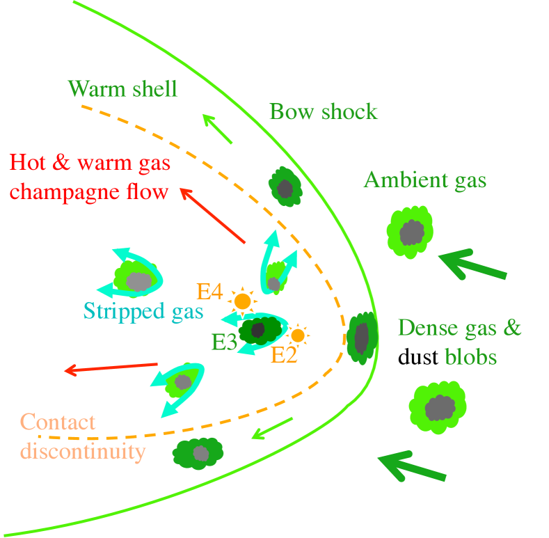
Figure 10: Illustration of the collision scenario between IRS 13E and the ambient medium through the plane of E2, E4, and the observer (roughly to the far left). Arrows mark the directions of gas motion relative to the mean velocity of E2 and E4. The illustrated objects are not meant to be properly scaled.

8.3 Emission structure within IRS 13E

The presence of dusty clumps in IRS 13E has been known for quite some time (e.g., Fritz et al., 2010). They are among the brightest and hottest non-stellar objects in the central parsec of the Galaxy and are clearly heated by the stars in the group. One possible origin of these clumps may be massive ejections from a star (e.g., E4), which could have left the luminous blue variable phase a short time ago (Coker et al., 2002). However, this scenario has multiple difficulties. 1) Such clumps should probably be distributed with some symmetry and have outward proper motions, the speed of which increases with the distance from the star because the entrainment by the fast stellar wind. The observed proper motions of the clumps show no such trends. 2) The time scale for the clumps to be advected out of IRS 13E by the wind, if the entrainment is efficient, is only $\sim 10{\rm~{}yr~{}v_{w,3}^{-1}}$, which may be far too short statistically to observe the clumps so near their star. 3) The velocity offset of E3.0 from E2 and E4 ($\sim 184{\rm~{}km~{}s^{-1}}$) is substantially greater than that from the bar ($\sim 88{\rm~{}km~{}s^{-1}}$). So E3.0 is more likely to originate from the bar than either of the two stars (see also Fritz et al., 2010).

In § 6.2, we have already mentioned the apparent connection between the central thermal emission peak (as seen in the ALMA observations) and the dusty clumps (observed in near-IR; Fritz et al. 2010). They show overall positional and morphological similarities, but also exhibit structural and kinematic variations. We speculate that the central thermal gas blobs and dusty clumps are physically associated. The dusty clumps are likely embedded within the warm gas blobs, which are heated by the stars. In our group wind collision scenario (§ 8.2; Fig. 10), the blobs represent the compressed dense substructures originating in the dense gas bar, similar to those seen in nearby HII regions  (e.g., Veena et al., 2017). The expected velocity evolution of the blobs naturally explains the observed variations in their kinematics: the systematic acceleration of the motion from west to east (Fritz et al., 2010) and the increasing blueshift of E3.0 with time (see § 7). Individual blobs are expected to suffer evaporation by ionizing radiation and stripping by fast-moving stellar wind material, which could account for the observed large LoS velocity spread. Both the pressure and the ionizing radiation intensity should be the highest in the region between E2 and E4, where blobs are expected to radiate brightly. Moreover, the rough thermal pressure balance (§ 7) is consistent with the interpretation of the mm and X-ray thermal emissions as arising from distributed and intermixed warm and hot gases in our scenario.

We have also considered the possibility for the formation of warm dusty gas directly from the cooling of shocked stellar wind material (Calderón et al., 2016; Calderón et al., 2019a). However, the separation between E2 and E4 is too large to reach high enough densities for the shocked wind material to cool down significantly, let alone to form dust.

8.4 Emission structures around IRS 13E

We first consider the observed X-ray emission from IRS 13E. In § 3, we have shown that the emission is predominantly thermal and most likely arises from the CW of the massive stars (chiefly E2 and E4) in the group. The characteristic temperature of 1.34 keV is well consistent with the expected speeds of the winds, and the pressure of the X-ray-emitting region is also consistent with that estimated in the warm dusty gas feature E3. However, the CW between the two stars alone has difficulties to explain the overall extent, fan-out morphology and softness of the X-ray emission, indicating that additional physical processes need to be accounted (§ 3).

Most naturally, we expect that the interaction of the group wind of IRS 13E with the surrounding gas plays a role (Fig. 10). We check how the interaction may be reflected in the X-ray properties of the group. First, the interaction should result in a partial confinement of the wind by the bow shock. Because of this confinement, the wind is expected to be reverse-shocked on the scale $r_{s}\sim(0.05{\rm~{}pc})\dot{M}_{w,-4}^{1/2}v_{w,8}^{1/2}n_{a,5}^{-1/2}v_{r.2}^{-1}$  (van Buren & McCray, 1988; Draine, 2011). The contact discontinuity of the reverse-shocked stellar wind material and bow shocked ambient gas should have a scale $r_{c}$ that is a factor of $\sim 1.5$ greater than $r_{s}$ (van Buren & McCray, 1988). We can reproduce the size of the shell ($r\sim 1\arcsec$) by approximating the combined stellar wind power in IRS 13E (Table 3) as a single source and adopting $v_{r}$ value in Table 1 and $n_{a,5}\sim 1$, consistent with the value estimated for the bar (Liszt, 2003; Tsuboi et al., 2017a). In reality, the structure of the contact discontinuity should certainly be considerably more complicated and should be elongated in the projected direction connecting E2 and E4. Second, the pressure gradient from the bow shock to the champagne flow should also result in a fan-out morphology of the X-ray emission, just as observed. Similarly, the emission from the CW between E2 and E4 should peak on the side facing the bow shock, which may explain the slightly westward offset ($\sim 0\aas@@fstack{\prime\prime}15$; § 3.1) of the X-ray emission peak. Third, the mass-loading of warm ionized gas into the hot gas can occur around individual dense blobs and at the contact discontinuity of the bow shock. The mass-loading naturally reduces the temperature of the hot gas, which should produce a softer spectrum than what is expected from the simple CW, as observed. If most of the extended X-ray emission is due to the cluster wind interaction with the bar, then the required increase of $\delta D$ can be reduced (see § 5). Correspondingly, $\dot{M}_{w}$ can also be lower than those quoted in Table 3 (the ”best fitted” and $\delta D=1\aas@@fstack{\prime\prime}3$ case). In short, the spatial and spectral properties of IRS 13E can be better explained by accounting for the interaction of the stellar winds with the ambient medium, in addition to the CW between E2 and E4.

We next consider the thermal emission from the ambient medium of IRS 13E. In the hydrogen Pa-$\alpha$ line emission map of the GC (Wang et al., 2010), we notice a shell-like structure around IRS 13E (Fig. 7C), in addition to its own emission which has been excised (Dong et al., 2012). This structure has an overall size of $\sim 2^{\prime\prime}$, comparable to that of the diffuse X-ray emission, is centered roughly at IRS 13E, and is elongated in the N-S direction, which is consistent with the orientation of E2 and E4. Therefore, most likely the structure represents the limb-brightened density enhancement of photo-ionized warm gas in the down-stream of the bow shock (Fig. 10). Furthermore, the western part of the structure is generally brighter and better defined than the eastern one, consistent with the bow shock morphology expected from the westward motion of IRS 13E relative to the ambient medium in the bar.

The Pa-$\alpha$ emission is relatively brighter than the average at the northern and southern ends. The shell-like structure is more well-defined on the western side than on the eastern side. However, the opposite is apparent in the H30$\alpha$ image. This difference may be explained by the differential attenuation of the Pa-$\alpha$ emission: higher on the eastern side than on the western one, while the H30$\alpha$ suffers no such effect. The H30$\alpha$ image shows no clear detection of the western shell-like structure, although patchy emission with large velocity offset and broadening is present (Component II discussed in § 6.2). This apparent overall morphological difference may be due to its lower detection sensitivity than the Pa-$\alpha$ one. The Pa-$\alpha$ intensity of the structure, as well as the apparent compact feature about 0$\aas@@fstack{\prime\prime}$7 further west, is $\lower 2.0pt\hbox{$\,\buildrel\scriptstyle<\over{\scriptstyle\sim}\,$}2\sigma$ above the background in the H30$\alpha$ image. The noise may also partly explain the lumpy appearance of the image, compared with the Pa-$\alpha$ image (see also § 6.2). Therefore, we tentatively suggest the presence of a shell-like structure, which is probably intrinsically brighter on the eastern side than on the western side.

In short, the CW and the ram-pressure confinement of the group wind by the ambient gas can naturally explain the structural, kinematic, and variability properties of dusty gas, as well as the X-ray emission, in and around IRS 13E.

8.5 Physical properties of warm ionized gas in IRS 13E

With the ALMA results, we now estimate such physical parameters as the temperature, density, and volume filling factor of warm ionized gas in the IRS 13E region. Assuming that that this gas is under the local thermodynamic equilibrium and its 232 GHz continuum and H30$\alpha$ line emissions are optically thin, the electron temperature $T_{\rm e}$ can be expressed as

$$T_{\rm e}({\rm K})=\left[\frac{6985}{\alpha(\nu,T_{\rm e})}\left(\frac{\nu}{\rm GHz}\right)^{1.1}\frac{1}{1+N({\rm He})/N({\rm H})}\times\left(\frac{S_{\rm C}}{S\Delta V_{\rm H30\alpha}}\right)\right]^{0.87},$$ (4)

where the elemental number density ratio of $N(\rm He)/N(\rm H)\sim 0.08$ and $\alpha(\nu,T_{\rm e})\sim 0.85$ at $\nu=232$ GHz and $T_{\rm e}\sim 10^{4}$ K (Mezger & Henderson, 1967). For E3, the total flux densities of the continuum and H30$\alpha$ line emissions are $S_{\rm C}=28.5\pm 1.8~{}{\rm mJy}$ and $S\Delta V_{\rm H30\alpha}=2.37\pm 0.12~{}{\rm Jy~{}km~{}s^{-1}}$. We thus have $T_{\rm e}=9260\pm 650$ K, which is consistent with previous estimates, ranging from 6000 K to 12000 K (Moser et al., 2017; Zhao et al., 2010; Tsuboi et al., 2019). We can also obtain the volume emission measure (EM) as (Murchikova et al., 2019)

$${\rm EM}=S\Delta V_{\rm H30\alpha}\frac{4\pi D^{2}}{\epsilon_{\rm H30\alpha}(T_{\rm e},n_{\rm e})}\frac{\nu}{c}\sim 1\times 10^{60}\rm~{}cm^{-3},$$ (5)

where the H30$\alpha$ emissivity $\epsilon_{\rm H30\alpha}=1.25\times 10^{-31}\rm~{}erg~{}s^{-1}$ for $T_{\rm e}=10^{4}$ K and $n_{\rm e}=10^{4}\sim 10^{7}\rm~{}cm^{-3}$ (Storey & Hummer, 1995) and the speed of light $c$ are used. Furthermore, we find that both the continuum and H30$\alpha$ emission intensities of E3 can be characterized by a Gaussian with a deconvolved size of $\sim 0.01$ pc, assuming a spherical symmetry. This together with the above EM value leads to the estimate of $n_{\rm e}\sim 3\times 10^{5}\rm~{}cm^{-3}f_{V}^{-1/2}$. By further assuming a thermal pressure balance between the warm and hot gases (e.g. $P/k\sim 2\times 10^{10}{\rm~{}K~{}cm^{-3}}$; § 3.2), we estimate the volume filling factor $f_{V}\sim 0.1$ and hence $n_{\rm e}\sim 10^{6}\rm~{}cm^{-3}$. If similar temperature and pressure could be assumed for warm ionized gas on larger scales, its filling factor has to be very small. We estimate that the total H30$\alpha$  flux within a circular region of 1^′′ radius centered on E3 (Fig. 7B) is $\sim 12\rm~{}Jy~{}km~{}s^{-1}$, which corresponds to ${\rm EM}=6\times 10^{60}\rm~{}cm^{-3}$. The filling factor is then $\sim 8\times 10^{-4}$, while the mass of the warm ionized gas in this region is $\sim m_{p}EM/n_{e}\sim 1\times 10^{-2}~{}M_{\odot}$. These estimates indicate that the volume is indeed dominated by hot gas and that warm gas traces dense clumps, probably their surfaces exposed to the ionizing radiation from massive stars in the region.

8.6 Potential effects of the group wind on larger scales

The interaction of the IRS 13E group wind with the surrounding medium should further occur on scales greater than the bow shock. The champagne flow, consisting of dusty warm clumps and hot gas, will eventually be terminated by the ram-pressure generated collectively by the outflow of Sgr A* (Wang et al., 2013), as well as winds from other stars in the GC cluster (Paumard et al., 2006). A quantitative study, however, requires a proper modeling of the champagne flow, which is not easy to do, because of its multi-phase nature. Nevertheless, we expect that a shock should terminate and eventually disperse the flow. A plausible intermediate product of this process is IRS 13N – a group of co-moving dusty objects located only about 0$\aas@@fstack{\prime\prime}$5 northeast of IRS 13E (Eckart et al., 2013).

Of course, high-speed collisions as experienced by IRS 13E, can also occur within other massive stars or groups. Such collisions may be a viable mechanism for dispersing dense gas in known organized streamers (Fig. 6). Gas and dust clumps or complexes have been observed to be scattered around Sgr A* (e.g., Eckart et al., 2013; Goicoechea et al., 2018). Their velocities generally do not match those of the streamers and arms. Such off-stream clumps could well represent remnants of dense gas blobs dispersed by similar encounters with massive stars.

9 Summary

We have conducted a detailed multi-wavelength study of IRS 13E and its vicinity, based primarily on archival Chandra and ALMA observations, as well as dedicated hydrodynamic simulations of the CW scenario. Our main results and conclusions are as follows:

• We find no significant change in X-ray properties of IRS 13E over a period of 15 years. The X-ray spectrum of IRS 13E, displaying distinct emission lines such as S, Si and Fe He-$\alpha$ transitions, can be well fitted with an optically-thin thermal plasma of a characteristic temperature $\sim 1.5\times 10^{7}$ K. The X-ray emission, with a 2-10 keV luminosity of $\sim 1.2\times 10^{33}{\rm~{}ergs~{}s^{-1}}$, is well resolved and has a size of about 2^′′. The X-ray emission has a fan-out global morphology; its centroid may be slightly offset ($\sim 0\aas@@fstack{\prime\prime}15$) from the effective center of the group toward the west – the direction of the group’s proper motion.

• No single known massive star (or potentially binary) in the group seems to dominate the X-ray emission. Assuming that a point-like source coincides spatially with the central peak of the emission, we constrain its luminosity as $\lower 2.0pt\hbox{$\,\buildrel\scriptstyle<\over{\scriptstyle\sim}\,$}6\times 10^{32}{\rm~{}ergs~{}s^{-1}}$ in the 2-10 keV band. A more physical consideration, based on an analogy to Sgr A*, shows that the luminosity of the IMBH, if present and undergoing hot accretion, should be orders of magnitude fainter.

• We detect for the first time the X-ray emission from the eclipsing X-ray binary E60, just 1$\aas@@fstack{\prime\prime}$3 away from IRS 13E. The emission also appears to arise from the CW of this binary. We find no indication for any interaction of the wind-wind collision between E60 and IRS 13E, indicating that they are not physically associated. This is consistent with the large LoS velocity difference between the two stellar systems.

• The X-ray emission of IRS 13E is dominantly due to shock-heated stellar winds from the massive stars, chiefly the two well-separated WR stars (E2 and E4), in the group. This CW scenario is consistent with the X-ray emission’s peak position between the WR stars. A comparison of the X-ray data with the simulations broadly confirms the scenario and provides interesting constraints on the wind parameters, as well as the physical separation between E2 and E4. The separation could be up to $\sim 1\aas@@fstack{\prime\prime}3$ (or 0.05 pc), about four times greater than the projected one, which would account for the bulk of the observed X-ray luminosity with quite nominal wind parameters. Nevertheless, even the best-matched model systematically under-predicts the X-ray intensity in $r\lower 2.0pt\hbox{$\,\buildrel\scriptstyle>\over{\scriptstyle\sim}\,$}0\aas@@fstack{\prime\prime}6$ regions. The predicted spectral shape is also somewhat harder than the observed, especially if the extinction-inferred high X-ray-absorbing gas column density is considered.

• From the consideration of the tidal radius of IRS 13E against the gravity of Sgr A*, we conclude that E1 is most likely not bound to the IRS 13E group, while E2 and E4 are physically associated. The combination of the gravitational bounding and the above best-matched separation of the two stars further suggests that the orbital distance of IRS 13E from Sgr A* is greater than 0.27 pc (equivalent to 7″) and/or that the mass of the group is primarily non-stellar. If the separation is much smaller than $\sim 1\aas@@fstack{\prime\prime}3$, then the extended X-ray emission needs to be primarily produced by the interplay between the IRS 13E group wind and the ambient medium located in the so-called bar of the minispiral around Sgr A*.

• The mm emission associated with IRS 13E is thermal and is well resolved spatially. The emission within the group is dominated by E3 – a complex of dusty clumps initially detected in near-IR and radio. Kinematically, this complex exhibits a broad LoS velocity spread up to $\sim 740{\rm~{}km~{}s^{-1}}$. The E3 complex further shows variation in both morphology and LoS speed on a 10 year time scale.

• We tentatively identify a shell-like Pa-$\alpha$-emitting structure of a dimension $\sim 2^{\prime\prime}$ and elongated in the north-south direction. This structure can be interpreted as the limb-brightened projection of the bow shock produced by the motion of IRS 13E relative to the bar. While the Pa-$\alpha$ emission is enhanced on the western side of the group, the diffuse H30$\alpha$ emission is on the eastern side.

• The impact of IRS 13E on the environment of Sgr A* is dynamic. With its energetic wind, IRS 13E can disturb the environment violently. Its strong ram-pressure can disperse dense gas in streams or arcs, potentially leading to sporadic cool gas inflows that feed Sgr A* (e.g., Murchikova et al., 2019).

These new constraints or insights on the presence of an IMBH, the stellar wind properties of the Wolf-Rayet stars, and their physical separation in IRS 13E, as well as its position relative to the minispiral bar and Sgr A*, are important for understanding the environment of Sgr A*. High spatial and timing resolution monitoring of the proper motions and kinematics of the region can be particularly useful to improve the constraints. Further modeling and simulations are needed to better quantify the results, especially the dynamics of the bar and its interplay with IRS 13E, and to further test the scenarios. Similar compact high-velocity features of dense gas observed in the GC may also be explained by such interplay with massive stellar winds – a phenomenon that may be quite common in galactic nuclear regions, where relative velocity between stellar groups and ambient medium can be very large, and may provide a mechanism to feed SMBHs sporadically with dense gas.

Appendix A ALMA channel maps of the H30$\alpha$ line emission in the IRS 13E region

References

- Arnaud (1996) Arnaud K. A., 1996, in Jacoby G. H., Barnes J., eds, ASP Conference Series Vol. 101, ADASS V. p. 17
- Arthur & Hoare (2006) Arthur S. J., Hoare M. G., 2006, ApJS, 165, 283
- Baganoff et al. (2001) Baganoff F. K., et al., 2001, Nature, 413, 45
- Banerjee & Kroupa (2011) Banerjee S., Kroupa P., 2011, ApJ, 741, L12
- Bartko et al. (2009) Bartko H., et al., 2009, ApJ, 697, 1741
- Calderón et al. (2016) Calderón D., Ballone A., Cuadra J., Schartmann M., Burkert A., Gillessen S., 2016, MNRAS, 455, 4388
- Calderón et al. (2019a) Calderón D., Cuadra J., Schartmann M., Burkert A., Prieto J., Russell C. M. P., 2019a, arXiv e-prints, p. arXiv:1906.04181
- Calderón et al. (2019b) Calderón D., Cuadra J., Schartmann M., Burkert A., Russell C. M. P., 2019b, arXiv e-prints, p. arXiv:1910.06976
- Capelli et al. (2012) Capelli R., Warwick R. S., Porquet D., Gillessen S., Predehl P., 2012, A&A, 545, A35
- Coker & Pittard (2000) Coker R. F., Pittard J. M., 2000, A&A, 361, L13
- Coker et al. (2002) Coker R. F., Pittard J. M., Kastner J. H., 2002, A&A, 383, 568
- Cuadra et al. (2008) Cuadra J., Nayakshin S., Martins F., 2008, MNRAS, 383, 458
- Cuadra et al. (2015) Cuadra J., Nayakshin S., Wang Q. D., 2015, MNRAS, 450, 277
- Cunha et al. (2007) Cunha K., Sellgren K., Smith V. V., Ramirez S. V., Blum R. D., Terndrup D. M., 2007, ApJ, 669, 1011
- Davies et al. (2009) Davies B., Origlia L., Kudritzki R.-P., Figer D. F., Rich R. M., Najarro F., 2009, ApJ, 694, 46
- Davis (2001) Davis J. E., 2001, ApJ, 562, 575
- Dong et al. (2011) Dong H., et al., 2011, MNRAS, 417, 114
- Dong et al. (2012) Dong H., Wang Q. D., Morris M. R., 2012, MNRAS, 425, 884
- Draine (2011) Draine B. T., 2011, Physics of the interstellar and intergalactic medium. Princeton University Press
- Eckart et al. (2013) Eckart A., et al., 2013, A&A, 551, A18
- Fritz et al. (2010) Fritz T. K., et al., 2010, ApJ, 721, 395
- Genzel et al. (2010) Genzel R., Eisenhauer F., Gillessen S., 2010, Reviews of Modern Physics, 82, 3121
- Goicoechea et al. (2018) Goicoechea J. R., Pety J., Chapillon E., Cernicharo J., Gerin M., Herrera C., Requena-Torres M. A., Santa-Maria M. G., 2018, A&A, 618, A35
- Liszt (2003) Liszt H. S., 2003, A&A, 408, 1009
- Maillard et al. (2004) Maillard J. P., Paumard T., Stolovy S. R., Rigaut F., 2004, A&A, 423, 155
- Martins et al. (2007) Martins F., Genzel R., Hillier D. J., Eisenhauer F., Paumard T., Gillessen S., Ott T., Trippe S., 2007, A&A, 468, 233
- Melia & Falcke (2001) Melia F., Falcke H., 2001, ARA&A, 39, 309
- Mezger & Henderson (1967) Mezger P. G., Henderson A. P., 1967, ApJ, 147, 471
- Mori et al. (2013) Mori K., et al., 2013, ApJ, 770, L23
- Mościbrodzka et al. (2006) Mościbrodzka M., Das T. K., Czerny B., 2006, MNRAS, 370, 219
- Moser et al. (2017) Moser L., et al., 2017, A&A, 603, A68
- Murchikova et al. (2019) Murchikova E. M., Phinney E. S., Pancoast A., Blandford R. D., 2019, Nature, 570, 83
- Nayakshin et al. (2007) Nayakshin S., Cuadra J., Springel V., 2007, MNRAS, 379, 21
- Paumard et al. (2001) Paumard T., Maillard J. P., Morris M., Rigaut F., 2001, A&A, 366, 466
- Paumard et al. (2006) Paumard T., et al., 2006, ApJ, 643, 1011
- Pfuhl et al. (2014) Pfuhl O., Alexander T., Gillessen S., Martins F., Genzel R., Eisenhauer F., Fritz T. K., Ott T., 2014, ApJ, 782, 101
- Portegies Zwart et al. (2006) Portegies Zwart S. F., Baumgardt H., McMillan S. L. W., Makino J., Hut P., Ebisuzaki T., 2006, ApJ, 641, 319
- Rathborne et al. (2014) Rathborne J. M., et al., 2014, ApJ, 795, L25
- Reid & Brunthaler (2004) Reid M. J., Brunthaler A., 2004, ApJ, 616, 872
- Roberts et al. (2017) Roberts S. R., Jiang Y.-F., Wang Q. D., Ostriker J. P., 2017, MNRAS, 466, 1477
- Russell et al. (2017) Russell C. M. P., Wang Q. D., Cuadra J., 2017, MNRAS, 464, 4958
- Schödel et al. (2005) Schödel R., Eckart A., Iserlohe C., Genzel R., Ott T., 2005, ApJ, 625, L111
- Schödel et al. (2009) Schödel R., Merritt D., Eckart A., 2009, A&A, 502, 91
- Schödel et al. (2014) Schödel R., Feldmeier A., Kunneriath D., Stolovy S., Neumayer N., Amaro-Seoane P., Nishiyama S., 2014, A&A, 566, A47
- Storey & Hummer (1995) Storey P. J., Hummer D. G., 1995, VizieR Online Data Catalog, p. VI/64
- Tsuboi et al. (2016) Tsuboi M., Kitamura Y., Miyoshi M., Uehara K., Tsutsumi T., Miyazaki A., 2016, PASJ, 68, L7
- Tsuboi et al. (2017a) Tsuboi M., Kitamura Y., Uehara K., Miyawaki R., Tsutsumi T., Miyazaki A., Miyoshi M., 2017a, ApJ, 842, 94
- Tsuboi et al. (2017b) Tsuboi M., Kitamura Y., Tsutsumi T., Uehara K., Miyoshi M., Miyawaki R., Miyazaki A., 2017b, ApJ, 850, L5
- Tsuboi et al. (2019) Tsuboi M., Kitamura Y., Tsutsumi T., Miyawaki R., Miyoshi M., Miyazaki A., 2019, PASJ, 71, 105
- Veena et al. (2017) Veena V. S., Vig S., Tej A., Kantharia N. G., Ghosh S. K., 2017, MNRAS, 465, 4219
- Verner et al. (1996) Verner D. A., Ferland G. J., Korista K. T., Yakovlev D. G., 1996, ApJ, 465, 487
- Wang et al. (1993) Wang Q. D., Li Z.-Y., Begelman M. C., 1993, Nature, 364, 127
- Wang et al. (2006) Wang Q. D., Lu F. J., Gotthelf E. V., 2006, MNRAS, 367, 937
- Wang et al. (2010) Wang Q. D., et al., 2010, MNRAS, 402, 895
- Wang et al. (2013) Wang Q. D., et al., 2013, Science, 341, 981
- Wilms et al. (2000) Wilms J., Allen A., McCray R., 2000, ApJ, 542, 914
- Yusef-Zadeh et al. (2015) Yusef-Zadeh F., Bushouse H., Schödel R., Wardle M., Cotton W., Roberts D. A., Nogueras-Lara F., Gallego-Cano E., 2015, ApJ, 809, 10
- Zhao & Goss (1998) Zhao J.-H., Goss W. M., 1998, ApJ, 499, L163
- Zhao & Goss (1999) Zhao J.-H., Goss W. M., 1999, in Falcke H., Cotera A., Duschl W. J., Melia F., Rieke M. J., eds, Astronomical Society of the Pacific Conference Series Vol. 186, The Central Parsecs of the Galaxy. p. 224
- Zhao et al. (2009) Zhao J.-H., Morris M. R., Goss W. M., An T., 2009, ApJ, 699, 186
- Zhao et al. (2010) Zhao J.-H., Blundell R., Moran J. M., Downes D., Schuster K. F., Marrone D. P., 2010, ApJ, 723, 1097
- van Buren & McCray (1988) van Buren D., McCray R., 1988, ApJ, 329, L93