Giant nonlocality in nearly compensated 2D semimetals

Abstract

In compensated two-component systems in confined, two-dimensional geometries, nonlocal response may appear due to external magnetic field. Within a phenomenological two-fluid framework, we demonstrate the evolution of charge flow profiles and the emergence of a giant nonlocal pattern dominating charge transport in magnetic field. Applying our approach to the specific case of intrinsic graphene, we suggest a simple physical explanation for the experimental observation of giant nonlocality. Our results provide an intuitive way to predict the outcome of future experiments exploring the rich physics of many-body electron systems in confined geometries as well as to design possible applications.

The trend towards miniaturization of electronic devices requires a deeper understanding of the electron flow in confined geometries. In contrast to the electric current in household wiring, charge flow in small chips with multiple leads may exhibit complex spatial distribution patterns depending on the external bias, electrostatic environment, chip geometry, and magnetic field. Traditionally, such patterns were detected using nonlocal transport measurements Skocpol et al. (1987); van Houten et al. (1989); Geim et al. (1991); Shepard et al. (1992); Hirayama et al. (1992); Mihajlović et al. (2009); Gorbachev et al. (2014), i.e. by measuring voltage drops between various leads other than the source and drain. Devised to study ballistic propagation of charge carriers in mesoscopic systems, these techniques were recently applied to investigate possible hydrodynamic behavior in ultra-pure conductors Bandurin et al. (2016, 2018); Berdyugin et al. (2019); Narozhny et al. (2017); Lucas and Fong (2018), where the unusual behavior of the nonlocal resistance is often associated with viscosity of the electronic system Torre et al. (2015); Levitov and Falkovich (2016); Falkovich and Levitov (2017); Pellegrino et al. (2017); Danz and Narozhny (2019).

Nonlocal resistance measurements have also been used to study edge states accompanying the quantum Hall effect McEuen et al. (1990); Wang and Goldman (1992); Roth et al. (2009); Abanin et al. (2011); Zhang et al. (2017); Komatsu et al. (2018). While the exact nature of the edge states has been a subject of an intense debate, the nonlocal resistance, $R_{NL}$, appears to be an intuitively clear consequence of the fact that the electric current flows along the sample edges and not through the bulk. Such a current would not be subject to exponential decay van der Pauw (1958) exhibited by the bulk charge propagation leading to a much stronger nonlocal resistance.

In recent years the focus of the experimental work on electronic transport has been gradually shifting towards measurements at nearly room temperatures Mihajlović et al. (2009); Abanin et al. (2011); Bandurin et al. (2016, 2018); Berdyugin et al. (2019). A particularly detailed analysis of the nonlocal resistance in a wide range of temperatures, carrier densities, and magnetic fields was performed on graphene samples Abanin et al. (2011). Remarkably, the nonlocal resistance measured at charge neutrality remained strong well beyond the quantum Hall regime, with the peak value ${R_{NL}\approx 1.5}\,$k$\Omega$ at ${B=12}\,$T and ${T=300}\,$K, three times higher than that at ${T=10}\,$K.

In this Letter, we argue that the giant nonlocality observed in intrinsic graphene at high temperatures can be attributed to the presence of two types of charge carriers (electrons and holes): at the neutrality point, the two bands (the conductance and valence bands) touch creating a two-component electronic system. Physics of such systems is much richer than in their single-component counterparts. Observed phenomena that are directly related to the two-band structure of the neutrality point include giant magnetodrag in graphene Gorbachev et al. (2012); Titov et al. (2013) and linear magnetoresistance Alekseev et al. (2015); Vasileva et al. (2016). Both effects have been explained within a phenomenological framework Titov et al. (2013); Alekseev et al. (2015) allowing for a two-component (electron-hole) system coupled by the external magnetic field. We generalize this approach to investigate evolution of the spatial distribution of the electron current density in the experimentally relevant Hall bar geometry. In sufficiently strong magnetic fields, the current density forms a giant nonlocal pattern where the current is flowing not only in the bulk, but also along the boundaries leading to strong nonlocal resistance, see Fig. 1. Such patterns can be directly observed in laboratory experiments using the modern imaging techniques Ella et al. (2019); Ku et al. (2019); Sulpizio et al. (2019). Tuning the model parameters to the specific values available for graphene, we arrive at a quantitative estimate of the nonlocal resistance Abanin et al. (2011).

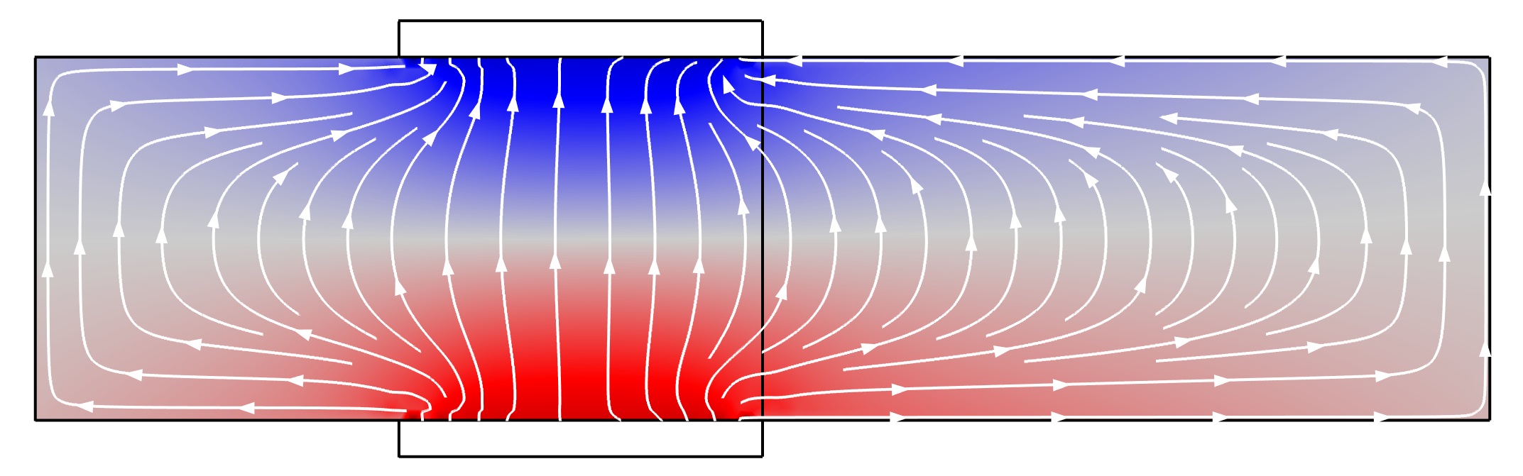
Figure 1: Giant nonlocality in a compensated semimetal in magnetic field. The arrows indicate the current flow and the color map shows the electrochemical potential (see the main text and Figs. 2 and 3 for specific parameters).

To highlight the difference between the one- and two-component systems, we briefly recall the macroscopic description of electronic transport in the standard (former) case. Allowing for nonuniform charge density, the linear relation between the electric current $\boldsymbol{J}$ and the external fields $\boldsymbol{E}$, $\boldsymbol{B}$ could be formulated as Lifshitz and Pitaevskii (1981); Narozhny et al. (2001); Danz and Narozhny (2019)

$$r_{0}\boldsymbol{J}=\boldsymbol{E}+r_{H}\boldsymbol{e}_{\boldsymbol{B}}\!\times\!\boldsymbol{J}+\frac{1}{e\nu_{0}}\boldsymbol{\nabla}n,$$ (1a)

where $$e>0 \nu_{0} n {\boldsymbol{e}_{\boldsymbol{B}}} r_{0} r_{H} {r_{H}=\omega_{c}\tau{r_{0}}} \omega_{c} \tau r_{0} r_{H}$$ is the unit charge, is the density of states (DoS), is the carrier density, is the unit vector in the direction of the magnetic field, and and are the longitudinal and Hall resistivities. Within the Drude-like description, ( is the cyclotron frequency and is the mean free path). The relation Eq. (1a) is applicable to a wide range of electronic systems from simple metals Ziman (1965); Giuliani and Vignale (2005) to doped graphene Katsnelson (2012); Narozhny et al. (2017). The transport coefficients and could be treated as phenomenological or could be derived from the underlying kinetic theory Narozhny et al. (2017); Narozhny (2019); Lifshitz and Pitaevskii (1981).

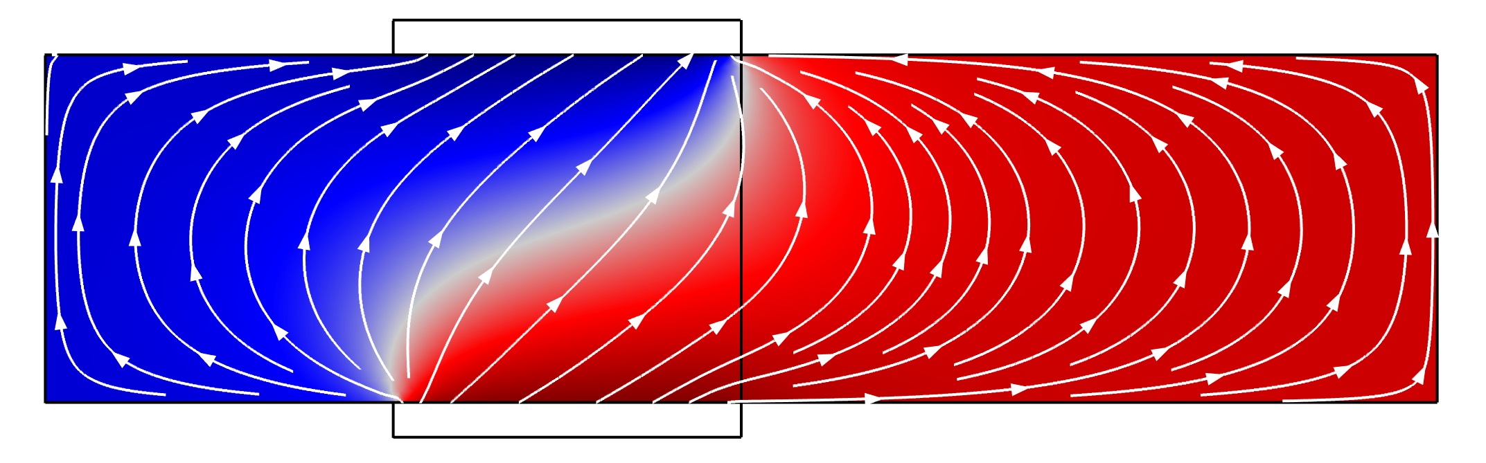
Figure 2: Classical Hall effect in a one-component electronic system. The current density (shown by the arrows) and the electrochemical potential (shown by the color map) were obtained from Eqs. (1) for a sample of the width $W=1\,\mu$m and length $L=4\,\mu$m with the carrier density $n=10^{12}\,$cm^-2 at the temperature $T=240\,$K and in magnetic field $B=0.2\,$T.

In addition to Eq.(1a), the electric current satisfies the continuity equation, which for stationary currents reads

$$\boldsymbol{\nabla}\!\cdot\!\boldsymbol{J}=0.$$ (1b)

Charge density inhomogeneity induces electric field, so that Eq. (1a) should be combined with the corresponding electrostatic problem. Most recent experiments were performed in gated structures, where the relation between the electric field and charge density simplifies Alekseev et al. (2015); Aleiner and Shklovskii (1994). In two-dimensional (2D) samples

$$\boldsymbol{E}=\boldsymbol{E}_{0}-\frac{e}{C}\boldsymbol{\nabla}n,$$ (1c)

where $C=\epsilon/(4\pi d)$ is the gate-to-sample capacitance per unit area, $d$ is the distance to the gate, $\epsilon$ is the dielectric constant, and $\boldsymbol{E}_{0}$ is the external field.

In a two-terminal (slab) geometry, solution of Eqs. (1) is a textbook problem. In the absence of magnetic field, the resulting electrochemical potential is governed by the relation of the mean free path to the system size, exhibiting either a flat (in short, ballistic samples) or linear (in long, diffusive samples) spatial profile. Most recently, these solutions were used as benchmarks in the imaging experiment Ella et al. (2019) and the numerical solution of the hydrodynamic equations in doped graphene Danz and Narozhny (2019). In external magnetic field, the system exhibits the classical Hall effect, which in short samples is accompanied by nontrivial current flow patterns Shik (1993).

In a four-terminal Hall bar geometry, the electric current still fills the whole sample, but decays exponentially van der Pauw (1958) away from the direct path between source and drain. The resulting flow pattern was calculated (in the context of doped graphene) in Refs. Levitov and Falkovich (2016); Falkovich and Levitov (2017); Danz and Narozhny (2019). In magnetic field, the pattern gets skewed due to the classical Hall effect, but exhibits no qualitatively new features, see Fig. 2.

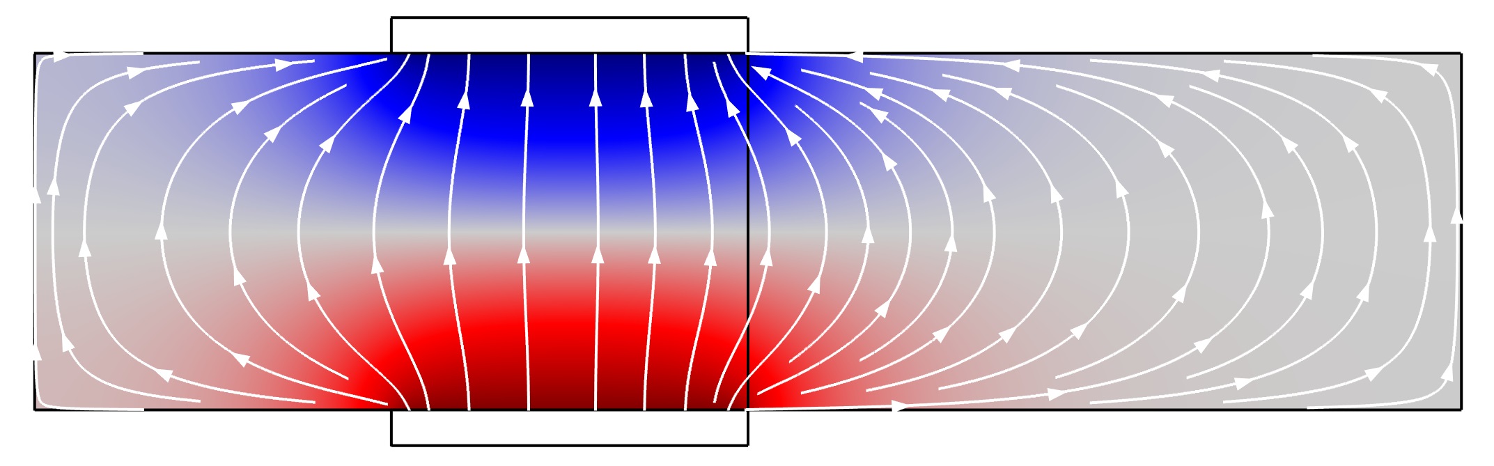
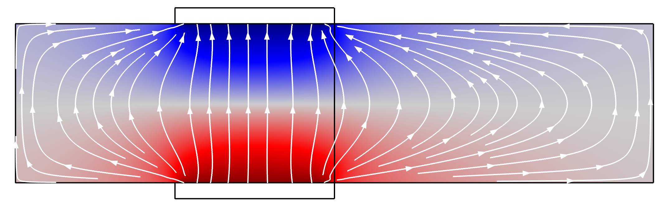
Figure 3: Charge flow in compensated semimetals. Top: Ohmic flow in the absence of magnetic field. Bottom: emergent nonlocality in weak magnetic field $B=0.2\,$T. The associated potential on the sample boundaries grows with the increasing field, see Fig. 1 for the pattern at $B=2\,$T. Stronger fields expel the current from the bulk such that it flows along the boundary.

Let us now extend the transport equations (1) to a two-component system. Keeping in mind applications to graphene, we re-write Eq. (1a) for the quasiparticles in the conduction band (“electrons”) in the form

$$-\boldsymbol{j}_{e}=eD\nu_{e}\boldsymbol{E}+\omega_{c}\tau\boldsymbol{j}_{e}\!\times\!\boldsymbol{e}_{\boldsymbol{B}}+D\boldsymbol{\nabla}n_{e},$$ (2a)

where $$\boldsymbol{j}_{e} {\boldsymbol{J}_{e}=-e\boldsymbol{j}_{e}} \nu_{e}$$ is the electron flow density (carrying the electric current ) and is DoS. The “holes” (i.e., the quasiparticles in the valence band) are described by

$$-\boldsymbol{j}_{h}=-eD\nu_{h}\boldsymbol{E}-\omega_{c}\tau\boldsymbol{j}_{h}\!\times\!\boldsymbol{e}_{\boldsymbol{B}}+D\boldsymbol{\nabla}n_{h}.$$ (2b)

Here the electric current carried by the holes is ${\boldsymbol{J}_{h}=e\boldsymbol{j}_{h}}$ and DoS may differ from that of electrons, ${\nu_{h}\neq\nu_{e}}$. For simplicity, we assume that the the cyclotron frequency, mean free time, and diffusion constant for the two bands coincide (a generalization is straightforward, but doesn’t lead to qualitatively new physics).

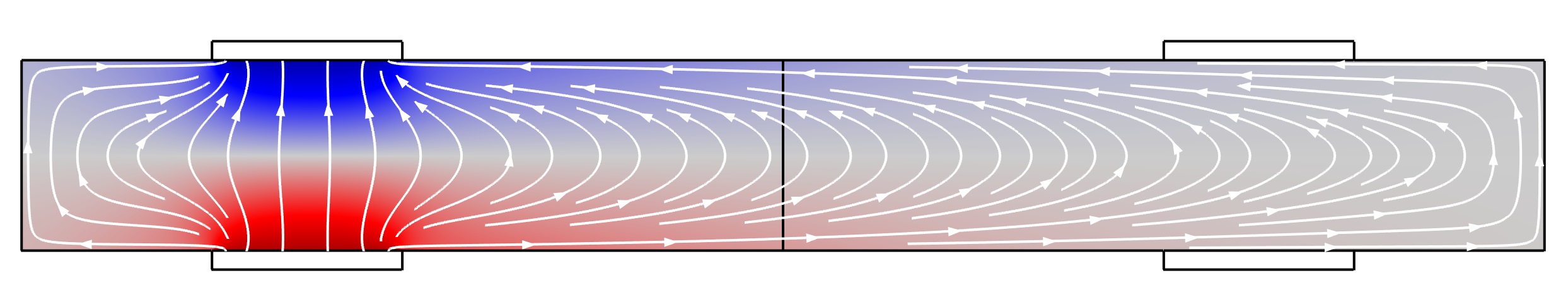
Figure 4: Giant nonlocality in the Hall bar geometry. The sample has a width ${W=1\,\mu}$m and length ${8\,\mu}$m, with the distance between contacts ${L=5\,\mu}$m. The driving current is ${I=0.1\,\mu}$A. The flow pattern was computed for ${B=0.8}\,$T, cf. Fig. 1.

The total electric current in the two component system is given by ${\boldsymbol{J}=-e\boldsymbol{j}}$, where ${\boldsymbol{j}=\boldsymbol{j}_{e}-\boldsymbol{j}_{h}}$. Introducing also the total quasiparticle flow ${\boldsymbol{j}_{I}=\boldsymbol{j}_{e}+\boldsymbol{j}_{h}}$, we find (cf. Ref. Narozhny (2019))

$$\boldsymbol{j}+eD(\nu_{e}+\nu_{h})\boldsymbol{E}+\omega_{c}\tau\boldsymbol{j}_{I}\!\times\!\boldsymbol{e}_{\boldsymbol{B}}+D\boldsymbol{\nabla}n=0,$$ (3a)

$$\boldsymbol{j}_{I}+eD(\nu_{e}-\nu_{h})\boldsymbol{E}+\omega_{c}\tau\boldsymbol{j}\!\times\!\boldsymbol{e}_{\boldsymbol{B}}+D\boldsymbol{\nabla}\rho=0,$$ (3b)

where $${n=n_{e}-n_{h}} -en {\rho=n_{e}+n_{h}}$$ is the carrier density per unit charge (the charge density being ) and is the total quasiparticle density. The transport equations have to be supplemented by continuity equations reflecting the particle number conservation. The electric current satisfies Eq. (1b), but the total number of quasiparticles Foster and Aleiner (2009) can be affected by electron-hole recombination processes leading to a weak decay term in the continuity equation

$$\boldsymbol{\nabla}\!\cdot\!\boldsymbol{j}_{I}=-\delta\rho/\tau_{R},$$ (3c)

where $\delta\rho$ is the deviation of the quasiparticle density from its equilibrium value and $\tau_{R}$ is the recombination time.

Under the assumption of electron-hole symmetry (e.g., at the charge neutrality point in graphene), ${\nu_{e}=\nu_{h}}$, we recover the phenomenological model of Ref. Alekseev et al. (2015). In the two-terminal geometry this model yields unsaturating linear magnetoresistance in classically strong fields Vasileva et al. (2016).

Now we analyze the behavior of the phenomenological model (3) in the four-terminal Hall bar geometry. In the absence of the magnetic field, the system exhibits a typical Ohmic flow Levitov and Falkovich (2016); Falkovich and Levitov (2017); Danz and Narozhny (2019), see the top panel in Fig. 3. Applying the field we find a qualitative change in the flow pattern – the emergence of a boundary flow and the associated electrochemical potential at the sample edges. Increasing the field leads to the nonlocal pattern growing until it fills the whole sample, see Figs. 1 and 4. Stronger fields essentially expel the current from the bulk with the charge flow being concentrated along the sample boundaries, which leads to strong nonlocal resistance.

The nonlocal flow pattern emerging in magnetic field, see Figs. 1, 3 and 4, has to be contrasted with the vortices appearing in the viscous hydrodynamic flow (e.g., in doped graphene Levitov and Falkovich (2016); Falkovich and Levitov (2017); Danz and Narozhny (2019); Xie and Levchenko (2019)). In the latter case, vorticity appears due to the constrained geometry of the flow and the particular boundary conditions Falkovich and Levitov (2017); Danz and Narozhny (2019); Kiselev and Schmalian (2019): neglecting Ohmic effects, the solution of the hydrodynamic equations can be obtained by introducing the stream function, which obeys a biharmonic equation independent of viscosity, which however affects the distribution of the electrochemical potential. In contrast, within the model (3) the “Ohmic” scattering represents the only source of dissipation and hence cannot be omitted. One can still introduce the stream function, but now it is determined not only by the sample geometry, but also by the Ohmic scattering and magnetic field. As a result, the flow pattern does not exhibit vortices, unlike those suggested recently for the hydrodynamic flow in intrinsic graphene Xie and Levchenko (2019) (in the absence of magnetic field).

Nonlocal resistance in graphene subjected to external magnetic field was studied experimentally in Ref. Abanin et al. (2011). At high enough temperatures where signatures of the quantum Hall effect are washed out, strong (or “giant”) nonlocality was observed at the neutrality point. The effect vanishes in zero field as well as with doping away from neutrality. Both features are consistent with the model (3): in zero field the model exhibits usual Ohmic flow patterns, see Fig. 3, while at sufficiently high doping levels the effects of the second band are suppressed – the two equations (3a) and (3b) become identical showing the response typical of one-component systems, see Fig. 2.

Having discussed the qualitative features of the charge flow in two-component systems, we now turn to a quantitative calculation of nonlocal resistance in graphene. Although the model (3) is applicable to any semimetal, graphene is a by far better studied material with readily available experimental values for model parameters. Here we use the data measured in Refs. Abanin et al. (2011); Gallagher et al. (2019); Bandurin et al. (2016, 2018); Titov et al. (2013) and theoretical calculations of Refs. Narozhny et al. (2017); Lucas and Fong (2018); Narozhny (2019); Titov et al. (2013); Xie and Levchenko (2019).

DoS of the quasiparticles in graphene has been evaluated in, e.g., Refs. Narozhny et al. (2017); Lucas and Fong (2018); Narozhny (2019); Katsnelson (2012), and has the form

$$\nu_{e}+\nu_{h}=2{\cal T}/(\pi v_{g}^{2}),\qquad\nu_{e}-\nu_{h}=2\mu/(\pi v_{g}^{2}),$$ (4)

where $\mu$ is the chemical potential, $v_{g}$ is the quasiparticle velocity in graphene, and ${{\cal{T}}=2T\ln[2\cosh(\mu/2T)]}$. The generalized cyclotron frequency is ${\omega_{c}=eBv_{g}^{2}/(c{\cal{T}})}$ and the diffusion coefficient has the usual form ${D=v_{g}^{2}\tau/2}$. At charge neutrality, ${\mu=0}$ and ${{\cal{T}}=2T\ln 2}$, while in the degenerate regime ${{\cal{T}}(\mu\gg{T})=\mu}$. The latter confirms that all coefficients in Eqs. (3a) and (3b) become identical with doping. Similarly, the continuity equations (1b) and (3c) should coincide in the degenerate regime. In graphene this happens by means of the fast decay of the recombination rate Titov et al. (2013). Close to neutrality we assume

$$\tau_{R}^{-1}=g^{2}T/\cosh(\mu/T),$$ (5)

where $g$ is determined by the corresponding matrix element. The above expression Titov et al. (2013) reflects the exponential decay of the two-band physics away from charge neutrality, which is responsible for the fast decay of $R_{NL}$ as a function of carrier density Abanin et al. (2011), see Fig. 5. Finally, the mean-free time, $\tau$, in graphene is a non-trivial function of temperature and carrier density Katsnelson (2012); Narozhny et al. (2017); Lucas and Fong (2018); Gallagher et al. (2019); Narozhny et al. (2012), which strongly depends on the model of the impurity potential Ando (2006); Shon and Ando (1998); Nomura and MacDonald (2006); Cheianov and Fal’ko (2006); Aleiner and Efetov (2006); Ostrovsky et al. (2006). However, these dependencies are typically not exponential and hence do not affect the exponential decay of the nonlocal resistance.

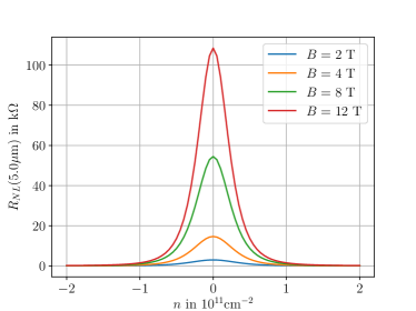
Figure 5: Nonlocal resistance measured in the Hall bar geometry, see Fig. 4, as a function of carrier density. Top: Coulomb scatterers; bottom: short-ranged impurities. The impurity model parameters are chosen to represent the mobility at ${n=10^{11}}\,$cm^-2 reported in Ref. Abanin et al. (2011). The range of magnetic fields and carrier densities as well as the distance to the gate (${d=50}\,$nm) is taken from Ref. Abanin et al. (2011), see Fig.2.

In Fig. 5 we demonstrate the decay of $R_{NL}$ for two impurity models – the Coulomb scatterers and short-ranged impurities – showing nearly identical behavior. Such robustness of the model (3) with respect of the functional dependence of the mean free time justifies the inaccuracy of our description of electronic transport in graphene, where close to charge neutrality the resistivity is strongly affected by electron-electron interaction. The data shown in Fig. 5 were obtained by solving Eqs. (3) in the Hall bar geometry of Fig. 4 using the estimate Xie and Levchenko (2019) for the recombination length scale, ${\ell_{R}=v_{g}\tau_{R}\approx 10\,\mu}$m (a previous calculation of Ref. Titov et al. (2013) put it at a smaller value $1.2\,\mu$m), which leads to similar results for the nonlocal resistance, but with a smaller peak value at charge neutrality.

The results for $R_{NL}$ shown in Fig. 5 are extremely similar to those reported in Ref. Abanin et al. (2011) with the exception of the values at neutrality, which are grossly exaggerated. There are several reasons for this behavior. Firstly, by ignoring the effects of electron-electron interaction, we strongly underestimate the usual resistivity of intrinsic graphene. Secondly, we ignore viscous effects. Furthermore, DoS in real graphene never really vanishes “at neutrality” due to electrostatic potential fluctuations Chiappini et al. (2016). As a result, the minimal carrier concentration is often as high as $10^{10}$cm^-2, essentially cutting off the lower density range around the peak in Fig. 5. Finally, Eq. (5) is a rather crude estimate that needs to be improved.

To conclude, we have argued that the observed giant nonlocality in neutral graphene in non-quantizing magnetic fields at relatively high temperatures observed in Ref. Abanin et al. (2011) is a direct consequence of the two-band nature of the quasiparticle spectrum in graphene. As such, this effect is not specific to graphene and should be observable in any compensated two-component system. Our theory does not involve spin-related phenomena including the effect of Zeeman splitting invoked in Ref. Abanin et al. (2011). The latter should be independent of the field direction, however, the effect was not observed in the nearly parallel field studied in Ref. Chiappini et al. (2016). Assuming the $g$-factor to be equal to $2$, we estimate the Zeeman splitting as ${E_{z}\approx 0.35}\,$meV${\approx 4}\,$K at ${B=10}\,$T. The corresponding residual quasiparticle density (at ${T=0}$) is given by ${\rho_{Q}=E_{z}^{2}/(4\pi v_{g}^{2})\approx 2.2\times 10^{6}}\,$cm^-2. As a result, we expect the effects of Zeeman splitting to be observable at temperatures and carrier densities much lower than those typical to nonlocal measurements discussed here.

With material-specific parameters, our phenomenological model is capable of a quantitative description of the effect. For graphene, a more precise calculation involving solution of the full system of hydrodynamic equations near charge neutrality is required to reach perfect agreement with the data, however the present approach shows that the effect is more general and does not require additional assumptions of electronic hydrodynamics.

The authors are grateful to I.V. Gornyi, A.D. Mirlin, J. Schmalian, J.A. Sulpizio, M. Schütt, A. Shnirman, and Y. Tserkovnyak for fruitful discussions. This work was supported by the German Research Foundation DFG within FLAG-ERA Joint Transnational Call (Project GRANSPORT), by the European Commission under the EU Horizon 2020 MSCA-RISE-2019 program (Project 873028 HYDROTRONICS), and by the Russian Science Foundation Project No. 17-12-0 (MT). BNN acknowledges the support by the MEPhI Academic Excellence Project, Contract No. 02.a03.21.0005.

References

- Skocpol et al. (1987) W. J. Skocpol, P. M. Mankiewich, R. E. Howard, L. D. Jackel, D. M. Tennant, and A. D. Stone, Phys. Rev. Lett. 58, 2347 (1987).
- van Houten et al. (1989) H. van Houten, C. W. J. Beenakker, J. G. Williamson, M. E. I. Broekaart, P. H. M. van Loosdrecht, B. J. van Wees, J. E. Mooij, C. T. Foxon, and J. J. Harris, Phys. Rev. B 39, 8556 (1989).
- Geim et al. (1991) A. K. Geim, P. C. Main, P. H. Beton, P. Streda, L. Eaves, C. D. W. Wilkinson, and S. P. Beaumont, Phys. Rev. Lett. 67, 3014 (1991).
- Shepard et al. (1992) K. L. Shepard, M. L. Roukes, and B. P. Van der Gaag, Phys. Rev. Lett. 68, 2660 (1992).
- Hirayama et al. (1992) Y. Hirayama, A. D. Wieck, T. Bever, K. von Klitzing, and K. Ploog, Phys. Rev. B 46, 4035 (1992).
- Mihajlović et al. (2009) G. Mihajlović, J. E. Pearson, M. A. Garcia, S. D. Bader, and A. Hoffmann, Phys. Rev. Lett. 103, 166601 (2009).
- Gorbachev et al. (2014) R. V. Gorbachev, J. C. W. Song, G. L. Yu, A. V. Kretinin, F. Withers, Y. Cao, A. Mishchenko, I. V. Grigorieva, K. S. Novoselov, L. S. Levitov, et al., Science 346, 448 (2014).
- Bandurin et al. (2016) D. A. Bandurin, I. Torre, R. Krishna Kumar, M. Ben Shalom, A. Tomadin, A. Principi, G. H. Auton, E. Khestanova, K. S. Novoselov, I. V. Grigorieva, et al., Science 351, 1055 (2016).
- Bandurin et al. (2018) D. A. Bandurin, A. V. Shytov, L. S. Levitov, R. K. Kumar, A. I. Berdyugin, M. Ben Shalom, I. V. Grigorieva, A. K. Geim, and G. Falkovich, Nat. Commun. 9, 4533 (2018).
- Berdyugin et al. (2019) A. I. Berdyugin, S. G. Xu, F. M. D. Pellegrino, R. K. Kumar, A. Principi, I. Torre, M. B. Shalom, T. Taniguchi, K. Watanabe, I. V. Grigorieva, et al., Science 364, 162 (2019).
- Narozhny et al. (2017) B. N. Narozhny, I. V. Gornyi, A. D. Mirlin, and J. Schmalian, Annalen der Physik 529, 1700043 (2017).
- Lucas and Fong (2018) A. Lucas and K. C. Fong, J. Phys: Condens. Matter 30, 053001 (2018).
- Torre et al. (2015) I. Torre, A. Tomadin, A. K. Geim, and M. Polini, Phys. Rev. B 92, 165433 (2015).
- Levitov and Falkovich (2016) L. Levitov and G. Falkovich, Nat. Phys. 12, 672 (2016).
- Falkovich and Levitov (2017) G. Falkovich and L. Levitov, Phys. Rev. Lett. 119, 066601 (2017).
- Pellegrino et al. (2017) F. M. D. Pellegrino, I. Torre, and M. Polini, Phys. Rev. B 96, 195401 (2017).
- Danz and Narozhny (2019) S. Danz and B. N. Narozhny (2019), eprint arXiv:1910.14473.
- McEuen et al. (1990) P. L. McEuen, A. Szafer, C. A. Richter, B. W. Alphenaar, J. K. Jain, A. D. Stone, R. G. Wheeler, and R. N. Sacks, Phys. Rev. Lett. 64, 2062 (1990).
- Wang and Goldman (1992) J. K. Wang and V. J. Goldman, Phys. Rev. B 45, 13479 (1992).
- Roth et al. (2009) A. Roth, C. Brune, H. Buhmann, L. W. Molenkamp, J. Maciejko, X.-L. Qi, and S.-C. Zhang, Science 325, 294 (2009).
- Abanin et al. (2011) D. A. Abanin, S. V. Morozov, L. A. Ponomarenko, R. V. Gorbachev, A. S. Mayorov, M. I. Katsnelson, K. Watanabe, T. Taniguchi, K. S. Novoselov, L. S. Levitov, et al., Science 332, 328 (2011).
- Zhang et al. (2017) X.-P. Zhang, C. Huang, and M. A. Cazalilla, 2D Materials 4, 024007 (2017).
- Komatsu et al. (2018) K. Komatsu, Y. Morita, E. Watanabe, D. Tsuya, K. Watanabe, T. Taniguchi, and S. Moriyama, Science Advances 4, eaaq0194 (2018).
- van der Pauw (1958) L. J. van der Pauw, Philips Tech. Rev. 20, 223 (1958).
- Gorbachev et al. (2012) R. V. Gorbachev, A. K. Geim, M. I. Katsnelson, K. S. Novoselov, T. Tudorovskiy, I. V. Grigorieva, A. H. MacDonald, S. V. Morozov, K. Watanabe, T. Taniguchi, et al., Nat. Phys. 8, 896 (2012).
- Titov et al. (2013) M. Titov, R. V. Gorbachev, B. N. Narozhny, T. Tudorovskiy, M. Schütt, P. M. Ostrovsky, I. V. Gornyi, A. D. Mirlin, M. I. Katsnelson, K. S. Novoselov, et al., Phys. Rev. Lett. 111, 166601 (2013).
- Alekseev et al. (2015) P. S. Alekseev, A. P. Dmitriev, I. V. Gornyi, V. Y. Kachorovskii, B. N. Narozhny, M. Schütt, and M. Titov, Phys. Rev. Lett. 114, 156601 (2015).
- Vasileva et al. (2016) G. Y. Vasileva, D. Smirnov, Y. L. Ivanov, Y. B. Vasilyev, P. S. Alekseev, A. P. Dmitriev, I. V. Gornyi, V. Y. Kachorovskii, M. Titov, B. N. Narozhny, et al., Phys. Rev. B 93, 195430 (2016).
- Ella et al. (2019) L. Ella, A. Rozen, J. Birkbeck, M. Ben-Shalom, D. Perello, J. Zultak, T. Taniguchi, K. Watanabe, A. K. Geim, S. Ilani, et al., Nat. Nanotechnol. 14, 480 (2019).
- Ku et al. (2019) M. J. H. Ku, T. X. Zhou, Q. Li, Y. J. Shin, J. K. Shi, C. Burch, H. Zhang, F. Casola, T. Taniguchi, K. Watanabe, et al. (2019), arXiv:1905.10791.
- Sulpizio et al. (2019) J. A. Sulpizio, L. Ella, A. Rozen, J. Birkbeck, D. J. Perello, D. Dutta, M. Ben-Shalom, T. Taniguchi, K. Watanabe, T. Holder, et al., Nature 576, 75 (2019).
- Lifshitz and Pitaevskii (1981) E. M. Lifshitz and L. P. Pitaevskii, Physical Kinetics (Pergamon Press, London, 1981).
- Narozhny et al. (2001) B. N. Narozhny, I. L. Aleiner, and A. Stern, Phys. Rev. Lett. 86, 3610 (2001).
- Ziman (1965) J. M. Ziman, Principles of the Theory of Solids (Cambridge University Press, Cambridge, 1965).
- Giuliani and Vignale (2005) G. Giuliani and G. Vignale, Quantum Theory of the Electron Liquid (Cambridge University Press, 2005).
- Katsnelson (2012) M. I. Katsnelson, Graphene (Cambridge University Press, 2012).
- Narozhny (2019) B. N. Narozhny, Annals of Physics 411, 167979 (2019).
- Aleiner and Shklovskii (1994) I. L. Aleiner and B. I. Shklovskii, Phys. Rev. B 49, 13721 (1994).
- Shik (1993) A. Shik, J. Phys. Condens. Matter 5, 8963 (1993).
- Foster and Aleiner (2009) M. S. Foster and I. L. Aleiner, Phys. Rev. B 79, 085415 (2009).
- Xie and Levchenko (2019) H.-Y. Xie and A. Levchenko, Phys. Rev. B 99, 045434 (2019).
- Kiselev and Schmalian (2019) E. I. Kiselev and J. Schmalian, Phys. Rev. B 99, 035430 (2019).
- Gallagher et al. (2019) P. Gallagher, C.-S. Yang, T. Lyu, F. Tian, R. Kou, H. Zhang, K. Watanabe, T. Taniguchi, and F. Wang, Science 364, 158 (2019).
- Narozhny et al. (2012) B. N. Narozhny, M. Titov, I. V. Gornyi, and P. M. Ostrovsky, Phys. Rev. B 85, 195421 (2012).
- Ando (2006) T. Ando, J. Phys. Soc. Jpn. 75, 074716 (2006).
- Shon and Ando (1998) N. Shon and T. Ando, J. Phys. Soc. Jpn. 67, 2421 (1998).
- Nomura and MacDonald (2006) K. Nomura and A. H. MacDonald, Phys. Rev. Lett. 96, 256602 (2006).
- Cheianov and Fal’ko (2006) V. V. Cheianov and V. I. Fal’ko, Phys. Rev. Lett. 97, 226801 (2006).
- Aleiner and Efetov (2006) I. L. Aleiner and K. B. Efetov, Phys. Rev. Lett. 97, 236801 (2006).
- Ostrovsky et al. (2006) P. M. Ostrovsky, I. V. Gornyi, and A. D. Mirlin, Phys. Rev. B 74, 235443 (2006).
- Chiappini et al. (2016) F. Chiappini, S. Wiedmann, M. Titov, A. K. Geim, R. V. Gorbachev, E. Khestanova, A. Mishchenko, K. S. Novoselov, J. C. Maan, and U. Zeitler, Phys. Rev. B 94, 085302 (2016).