The entanglement membrane in chaotic many-body systems
Abstract
In certain analytically-tractable quantum chaotic systems, the calculation of out-of-time-order correlation functions, entanglement entropies after a quench, and other related dynamical observables, reduces to an effective theory of an “entanglement membrane” in spacetime. These tractable systems involve an average over random local unitaries defining the dynamical evolution. We show here how to make sense of this membrane in more realistic models, which do not involve an average over random unitaries. Our approach relies on introducing effective pairing degrees of freedom in spacetime, describing a pairing of forward and backward Feynman trajectories, inspired by the structure emerging in random unitary circuits. This provides a framework for applying ideas of coarse-graining to dynamical quantities in chaotic systems. We apply the approach to some translationally invariant Floquet spin chains studied in the literature. We show that a consistent line tension may be defined for the entanglement membrane, and that there are qualitative differences in this tension between generic models and “dual-unitary” circuits. These results allow scaling pictures for out-of-time-order correlators and for entanglement to be taken over from random circuits to non-random Floquet models. We also provide an efficient numerical algorithm for determining the entanglement line tension in 1+1D.
I Introduction
This paper is about universality in the dynamics of chaotic many-body systems. One familiar type of universality is encapsulated in hydrodynamics for conserved quantities and other slow modes kadanoff_hydrodynamic_1963 ; hohenberg1977theory . But random circuits oliveira2007generic ; hamma2012quantum ; brandao2016local ; nahum_quantum_2017 ; nahum_operator_2017 ; von_keyserlingk_operator_2017 ; rakovszky_diffusive_2017 ; khemani_operator_2017 ; chan_solution_2018 ; chan_spectral_2018 ; rowlands2018noisy ; zhou2019emergent ; rakovszky_sub-ballistic_2019 ; friedman_spectral_2019 ; hunter-jones_unitary_2019 , a family of tractable many-body systems, have suggested new aspects of universality nahum_quantum_2017 ; nahum_operator_2017 ; von_keyserlingk_operator_2017 ; rakovszky_diffusive_2017 ; khemani_operator_2017 ; chan_solution_2018 ; zhou2019emergent . In particular they have revealed a generic structure associated with an emergent “membrane” in spacetime nahum_quantum_2017 ; jonay_coarse-grained_2018 . The effective statistical mechanics of this membrane determine the production of entanglement after a quantum quench, the spreading of quantum operators, and other aspects of the “scrambling” lieb_robinson ; calabrese2005evolution ; kim2013ballistic ; kitaev2014hidden ; liu2014entanglement ; shenker_black_2014 ; roberts2015localized ; maldacena_bound_2015 ; roberts_lieb-robinson_2016 ; kaufman2016quantum ; aleiner2016microscopic ; patel2017quantum ; hosur_chaos_2016 ; mezei2017entanglement2 ; nahum_operator_2017 ; von_keyserlingk_operator_2017 ; chan_solution_2018 ; kos2017many ; mezei_exploring_2019 of quantum information.
One way to motivate this membrane, which is relevant to the approach we take here, is via the multi-layer structure of the quantum circuit (or the multi-sheet structure of the path integral, in a continuum language) representing the observables in question. Algebraically, conventional correlation functions, such as an expectation value following a quench, involve a single copy of the unitary time evolution operator , and a single copy of its Hermitian conjugate . Formally, we can represent them in terms of matrix elements of the operator . But the quantities mentioned above (for example the th Rényi entropy, obtained by tracing the th power of the reduced density matrix) require matrix elements of the multiply “replicated” operator
| (1) |
with copies of , and copies of . In a path integral language, we require multiple forward and backward paths calabrese2005evolution ; maldacena_bound_2015 .
The structure arising from this is most easily understood in random unitary circuits, which are chaotic models built from random unitary gates nahum_quantum_2017 ; nahum_operator_2017 ; von_keyserlingk_operator_2017 ; chan_solution_2018 ; zhou2019emergent . Averaging in Eq. 1 over the random unitaries introduces a degree of freedom , at each location in spacetime, that labels a pairing between the set of forward replicas and the set of backward replicas, i.e. a pairing of trajectories zhou2019emergent . Formally this pairing is a permutation, , and quantities like the Rényi entropies and the out-of-time ordered correlator (OTOC) map to effective partition functions for . In this setting, the membrane can be understood as a domain wall between different values of the pairing field nahum_operator_2017 ; chan_solution_2018 ; zhou2019emergent .
The goal of this work is to show how to make sense of the pairing field and the membrane in nonrandom systems. This allows the language of the renormalization group to be applied to chaotic dynamics.


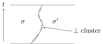
The basic quantity characterizing the membrane is its coarse-grained “line tension” jonay_coarse-grained_2018 . This line tension determines the system’s butterfly velocity or operator spreading speed and its entanglement growth rate. It can be thought of loosely as associating an entanglement cost with a given curve in spacetime (in general this tension depends on ). See Fig. 1 for a schematic picture.
We expect that the pairings, and the membrane description, continue to make sense in systems more general and more realistic than random circuits, for the heuristic reason described in the next paragraph. In support of this, there is numerical evidence that a consistent membrane tension can be defined in a generic spin chain jonay_coarse-grained_2018 , and in a dual-unitary circuit bertini_entanglement_2018 ; piroli_exact_2019 . There are analytic computations in random Floquet circuits in the large Hilbert space dimension (large ) limit chan_solution_2018 , showing that the domain wall structure makes sense in that limit. Finally, there is an analytical derivation of the form of the membrane tension in holographic systems mezei2018membrane ; mezei_exploring_2019 , at leading order in the number of degrees of freedom; this also begins to make a concrete connection between the entanglement membrane, and the Ryu-Takayanagi/Hubeny-Rangamani-Takayanagi geometrical pictures for entanglement in AdS space ryu2006holographic ; hubeny2007covariant ; agon2019bit ; freedman_bit_2017 . (Lattice toy models for the AdS-CFT correspondence, using random tensor networks, also exhibit domain walls between permutation degrees of freedom hayden2016holographic ; vasseur2018entanglement .) But at present there is no formalism for explaining how the pairing degrees of freedom emerge when there is no average over randomness, or how to compute the properties of the membrane in a generic system without randomness and away from any large--like limit. As a more general point, random circuits and related stochastic models have shed light on various aspects of chaotic dynamics nahum_quantum_2017 ; nahum_operator_2017 ; von_keyserlingk_operator_2017 ; rakovszky_diffusive_2017 ; khemani_operator_2017 ; chan_solution_2018 ; rowlands2018noisy ; zhou2019emergent ; rakovszky_sub-ballistic_2019 ; chan_spectral_2018 ; friedman_spectral_2019 ; hunter-jones_unitary_2019 , and a natural question is how to generalize these calculations to non-random systems. Our aim here is to provide a formalism for doing this.
Heuristically, the paired configurations mentioned above can be thought of as saddle points of the path integral for the replicated evolution operator (1). This path integral contains multiple forward and backward paths. In a continuum language, these are weighted by and respectively, where is the action; in the discrete setting, is replaced by a product of matrix elements of local unitaries. By pairing each forward path with a backward path we can cancel the phases in the exponent, so we might guess that paired configurations predominate. In the cases of interest to us, however, the boundary conditions force the pairing to differ in different regions of spacetime. This leads to saddle-point solutions with a nontrivial membrane structure.
In this work we show explicitly, for a large class of systems without conservation laws, how the pairing field and the entanglement membrane emerge, making the above heuristic picture precise. We emphasize that we do not require either a limit of large local Hilbert space dimension, or any kind of randomness. To demonstrate the utility of our approach, we compute the entanglement line tension (for , the case relevant to the OTOC and to the second Rényi entropy) for a variety of translationally-invariant Floquet spin-1/2 chains.
Formally, our approach is to work in the replicated Hilbert space (acted on by Eq. 1) and to insert, in each time slice, an exact local resolution of identity. This includes states associated with pairings, but also a projector onto the complementary part of the Hilbert space, which we denote by , containing non-pairing states. Traces of , yielding for example correlation functions or Rényi entropies, can then be written as partition functions for an effective “spin” which can take the values either (a permutation) or .
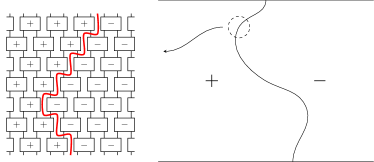
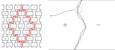
Including these non-pairing states allows the structures that appear in the random circuit to be generalized to models without any random average. The Haar-averaged random circuit can be thought of as a special case: there, the contribution from any spin configuration that includes a vanishes after averaging, leaving a spin model for permutations only, and the membrane is a domain wall between permutations nahum_operator_2017 ; zhou2019emergent . In, say, a translationally-invariant system, the domain wall structure becomes more complex, with the appearance of the spin value along the domain wall. (In fact, this is also true in a particular realization of the random circuit, before we average over the random unitaries.) This leads to a thickened domain wall with a more complex structure. However we argue that in chaotic systems, the domain wall’s width remains of order 1 in terms of microscopic lengthscales. Therefore, on large scales, the membrane is still well-defined, but with a nontrivial, renormalized membrane tension function. We illustrate this situation in Fig. 2.
Our initial introduction of the pairing field is exact but formal, because the microscopic weight for a configuration is in general complicated. To make progress we first argue that configurations with large unpaired regions (large regions of ) are exponentially suppressed. Then we show how to resum an infinite number of configurations, or “Feynman diagrams”, exactly, to give a simpler description of the entanglement membrane, in terms of a reduced set of parameters.
This is loosely analogous to the renormalization of the mass of a quasi-particle due to interactions — here the states dress the structure of the membrane, giving it a larger width (than in the averaged random circuit, where states are suppressed) and a modified line tension. This is an application of the renormalization group idea to find the coarse grained quantities characterizing scrambling.
Before tackling translation-invariant systems, we analyze the case of a fixed realization of a random unitary circuit. This illustrates the basic mechanism that makes the approach possible — suppression of states by phase cancellation — in a tractable setting. Since the disorder realization is fixed, we cannot introduce the pairing degrees of freedom by Haar-averaging. Instead we apply the new method described here. Working at large but finite Hilbert local space dimension, we show that the membrane remains well-defined, and is thickened slightly by occasional appearances of states. This leads to a membrane that inhabits a disordered “potential” in spacetime. This picture reproduces our previous results on Kardar-Parisi-Zhang (KPZ) fluctuations in the Rényi entropy between different realizations of the random circuit zhou2019emergent . But previously these results required the replica trick, which we are able to dispense with here.
Next we turn to Floquet dynamics of spin- chains, without any kind of randomness. In order to control the calculations, we introduce a systematic expansion in the maximal temporal extent of connected clusters in the effective spin model. A priori, this expansion does not have a small parameter. However we conjecture (based on the tractable case of the random circuit), and give numerical evidence, that it is a convergent expansion in chaotic Floquet systems.
Using this observation, we construct an efficient numerical scheme for computing the membrane line tension using the expansion above: we truncate the maximum size of a connected cluster (but we do not require that these clusters are dilute), and we examine convergence as a function of the order at which we truncate. We first discuss Floquet models with a local unitary circuit structure, since these are the simplest case to visualize. However the circuit structure is not required: we also apply the method to completely generic Floquet models, involving Hamiltonian evolution in continuous time without any circuit structure.
The numerical results show good convergence for a wide range of chaotic models, including prototypical spin models for quantum chaotic systems, such as Floquet Ising models with longitudinal and transverse fields (kicked Ising models) kim2013ballistic ; kim_testing_2014 ; prosen_chaos_2007 .
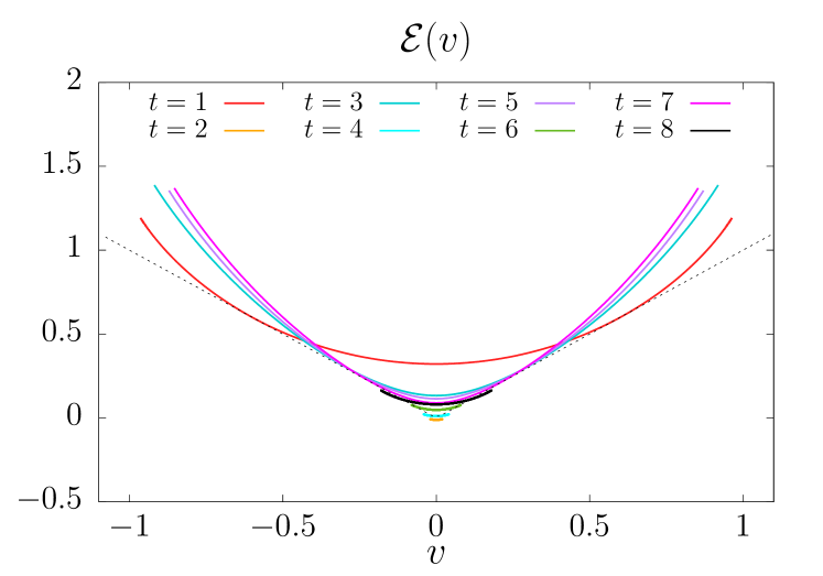
The line tension satisfies some general constraints jonay_coarse-grained_2018 which provide a highly nontrivial check on our results. Recall that is proportional to the “free energy”, in the scaling limit, of a membrane whose shape is parameterized by (Fig. 1). is a convex function of velocity, which is tangential to the line at the point , where is the quantum butterfly velocity (for parity symmetric systems): see the schematic picture in Fig. 1. For the chaotic systems we study, our numerical approximations to indeed appear to converge a form satisfying the constraints above.
We also investigate a special case of the kicked Ising model that has maximal entanglement growth bertini_entanglement_2018 ; piroli_exact_2019 and the property of “dual unitarity” which, remarkably, allows a range of exact computations gopalakrishnan_unitary_2019 ; bertini2019exact ; akila_particle-time_2016-2 ; bertini2019operator ; piroli_exact_2019 .
In addition to studying particular models, we discuss the general continuum theory for the membrane in 1+1D. We argue that the entanglement membrane has special properties in dual-unitary circuits: its equation of motion becomes a wave equation, rather than being diffusive as it is in generic models.
I.1 Organization of the paper
Sec. II introduces pairing degrees of freedom in the multi-layer unitary circuit, leading to an effective spin model (Sec. II.1–II.3) in which a domain wall structure emerges (Sec. II.4).
We first test our formalism in an analytically tractable setting, a fixed realization of a random circuit, in Sec. III. We show that large clusters of in the effective spin model are exponentially suppressed (Sec. III.1) and use this to obtain Kardar-Parisi-Zhang scaling of the Rényi entropy (Sec. III.2).
We then develop a systematic formalism for resumming the effect of clusters for translationally invariant Floquet circuits. Sec. IV describes technical preliminaries, and Sec. V applies the method to various models from the literature. Sec. VI discusses the coarse-graining of the membrane, showing that two distinct universality classes arise, for a generic circuit and a self-dual circuit.
We discuss the application of this formalism to operator spreading in Sec. VII, and to general Floquet models in continuous time, without any circuit structure, in Sec. VIII.
Sec. IX describes some open questions. Appendices contain technical details about the spin model and further numerical results.
II Defining the spin model

For concreteness, let us focus on time evolution with a unitary circuit made of two-site gates, with the structure in Fig. 3. (The constructions below generalize straightforwardly to evolution without a circuit structure: we describe this explicitly in Sec. VIII.) We will use or simply to denote the full many-body unitary represented by the entire circuit, and the lower-case to stand for a local two-site gate.
At this point the local gates are left arbitrary. In some sections we will restrict to Floquet models with both space and time translation invariance, but this is not necessary. The circuit geometry guarantees that there is no propagation of information outside a strict lightcone with speed ; the actual butterfly speed in these circuits is in general strictly smaller than 1.
Conventional time ordered correlation functions such as involve a ‘two-layer’ quantum circuit made of and , in the sense that they can be obtained from the contraction of by inserting operators in the intermediate time-steps (here is the complex conjugate of , taken in an arbitrary local basis, and not the Hermitian conjugate). In contrast, the quantities of interest to us here require traces of the -layer unitary circuit
| (2) |
where . For example, the out-of-time order correlation function
| (3) |
requires . The Rényi entanglement entropy for subsystem
| (4) |
requires to write the -th power of the time-evolved reduced density matrix.
Taking leads to new structure. One consequence is that it multiplies the number of conservation laws, since formally each ‘copy’ of the system undergoes independent unitary evolution. This will not concern us here, however, since we study models without conservation laws. The additional structure we examine is instead associated with pairings between spacetime histories in the ‘worlds’ associated with different layers zhou2019emergent .
The multi-layer circuit has layers of and of , and can be thought of as describing evolution of a ‘replicated’, multi-copy system. For a heuristic picture, we may think in terms of Feynman histories of this replicated system in our chosen local basis. The amplitude for a given Feynman history is given by a product of matrix elements of the local unitaries. Feynman histories that are ‘paired’, so that the histories occuring in the replicas are pairwise equal to the histories occuring in the replicas, avoid phase cancellation zhou2019emergent . (This pairing can happen in different ways.) We will argue that in quantum chaotic systems, the observables mentioned above are dominated by Feynman histories that have a well-defined pairing structure after coarse-graining. We will show how a corresponding local ‘pairing field’ can be defined by coarse-graining over microscopic length and time scales.
II.1 Introducing the effective spins
To motivate the structures we will consider, we first recall what happens when the local unitaries are averaged over the Haar ensemble instead of being fixed.
For a given two-site gate , acting on sites and , the replicated gate is a unitary operator on copies ( layers of , layers of ) of the two-site Hilbert space, which has dimension . Its average (which is no longer unitary) is the operator
| (5) |
where Wg is the unitary Weingarten function collins_integration_2006 ; gu_moments_2013 ; weingarten1978asymptotic . Here and are elements of the permutation group . These denote a pairing of the layers, labelled , with the layers, labelled . For example corresponds to pairing with , etc. At a given spatial site, the state is a product of maximally entangled states between paired copies of the site, and the states above are for a pair of spatial sites: .
For example, for , there are two possible permutations: the identity, , and the transposition, denoted in cycle notation. In our local basis the corresponding states at a site are
| (6) | ||||
(note that we do not normalize these states).
In Ref. zhou2019emergent, we showed how, starting with the above expression, the expression for could be reduced to a lattice magnet, with local interactions, for the permutations (the permutations were integrated out in this mapping). At the end of this mapping, there is a single spin associated with each local block in the circuit.
Now let us consider a general circuit with the brickwork geometry in Fig. 3. The basic idea will be to separate out the pairing (permutation) states, , in the multi-copy Hilbert space for a pair of sites, from states in orthogonal complement of this space.
Regardless of the choice of unitary gate, we will be able to decompose the multi-layer unitary as
| (7) |
where is a projection operator onto paired states, which as discussed below is also equal to , and “” represents the projection of to the complement of the space of paired states. Eq. 5 shows that in the Haar-averaged case the “” contributions vanish identically. More generally they do not vanish, and their operator norm is not negligible. However we will argue that the permutation states dominate in a certain sense, and that states in the orthogonal complement can be taken into account via a systematic procedure.
The expression for the Haar average of a local unitary in Eq. 5 can be regarded simply as the projection operator onto the subspace of permutation states. By the invariance of the Haar measure under (say) left multiplications,
| (8) |
showing that this is a projector. The state satisfies for any choice of two-site unitary, so after Haar averaging we also have
| (9) |
for any permutation . This shows that the Haar averaged object, which is a Hermitian operator on the replicated space, is equal to , the orthogonal projector onto the subspace spanned by permutation states harrow_church_2013 .
To separate out contributions from permutation states for a general circuit, we will insert the resolution of the identity (on two physical sites)
| (10) |
immediately before each two-site gate in the circuit. Here is the projector onto the subspace complementary to that spanned by pairing states. This insertion is shown in (11) below as a bar below each gate.
We will view the quantity to be computed, for example the purity, as a partition function which we denote . (In the purity example, the second Rényi entropy is the free energy associated with this partition function.) After using 10, this partition function is a sum of terms with all possible choices of projection operator inserted below each gate. Graphically,
| (11) |
where the sum is over all possible assignments of to the projection operators, which are represented by horizontal bars. We leave the boundary conditions at the initial and final times unspecified at this point, since they depend on the observable to be computed.
Note that the operator can “absorb” an arbitrary two-site gate. This can be seen from the invariance of the Haar measure. For any 2-site unitary ,
| (12) |
As a result, the term in the partition function where all the insertions are is identical to the expression where all gates are replaced with Haar-averaged gates. Therefore the decomposition in Eq. 11 gives us a well-understood starting point, which we can go beyond by taking into account domains of insertions. Roughly speaking, this approach will be useful if these domains do not form a connected cluster ‘percolating’ from the top to the bottom of the spacetime slab, but instead form finite clusters. Their effect can then be taken into account as a renormalization of the interactions for the permutation degrees of freedom that are present in the random circuit.
To make these permutations explicit we decompose using Eq. 5. In the random circuit it was useful to perform the sum over the variables (cf. Eq. 5) explicitly, leaving a partition sum solely for the variables. Algebraically, that corresponds to splitting into projection operators ,
| (13) |
which are given by grouping together terms in Eq. 5 with a given :
| (14) |
Using the properties of the Weingarten function, one can check that the states appearing in the brackets
| (15) |
form the dual basis of , i.e. , so that the non-Hermitian operators are projectors satisfying (App. A.1):
| (16) |
Here we assume that is generic, to avoid divergences in the Weingarten function, which can arise for small values of when is sufficiently large (for , such divergences can arise for ). This is not a fundamental obstacle, as we could always define a “spin” with a larger local Hilbert space dimension by grouping sites.
Our resolution of the identity, inserted below each block in the multi-layer circuit, is now refined to
| (17) |
Let us represent the possibilities graphically as:
| (18) |
Importantly, the blocks on the left, labelled by permutations, are independent of the choice of local unitary gate, because again “absorbs” any unitary. For any gate , we have , so
| (19) |
However the blocks, which represent the tensor , depend on the local unitaries defining the dynamics.
We have now written as a sum over spins , associated with each block in the circuit, which take values in :
| (20) |
Throughout this paper, we will use to label the bond between two lattice sites. The gates are located on half of the bonds.
Note that “” is simply a choice of label for one of the values that can take; we could also have denoted this state by “” or anything else. At each location, runs over different values.
The weight of a spin configuration in this partition sum is given by contracting the network. In general, this weight is not simply a product of local terms. However we will argue that for the boundary conditions of interest, and for generic models, there is an effective notion of locality. We first describe some basic properties of the weights (Secs. II.2, II.3), and then specify to the case of interest, where the boundary conditions induce a domain wall structure in the spin configuration (Sec. II.4).
II.2 General properties of the spin model
First consider the sub-partition-function without any insertions (i.e. with everywhere), which we denote .
is a statistical model whose “spins” are permutations zhou2019emergent . The spins have local three-body interactions on “down-pointing triangles” (and no interactions on up-pointing triangles). To be specific, each down-pointing triangle such as
| (21) |
has an associated weight
| (22) |
From Eq. 14, the interaction triangle is (see App. A.1)
| (23) |
Equivalently, the triangle is the coefficient in the expansion
| (24) |
where the two arguments in the bras refer to the pair of spatial states.
This spin model was described in Ref. zhou2019emergent, for the random circuit. In that context, the spins arose from the Haar average over the physical random unitary in Eq. 5. The three-body interaction appears after integrating out the “” spins. Here the sum over the spins appeared at the state level in defining the projection operator in Eq. 14.
The simplest case is nahum_operator_2017 . There are then two possible permutations, and , which we denote and . The weights are symmetric under exchange of and and under spatial reflection. They are
| (25) |
with
| (26) |
which follows from Eq. 14 with the explicit expression
| (27) | ||||
and symmetrically for .
Note the vanishing of the first weight, which amounts to a hard constraint on the spin configurations. The spin configuration is in fact highly constrained for any : the underlying unitarity means that vanishes for many configurations of the triangle. In other words, many terms in the sum over defining are zero (see Ref. hunter-jones_unitary_2019 and App. A.2 for a further simplification). For example, as a generalization of the first equality in Eq. 25 above,
| (28) |
This enforces a light cone structure. For example, for the purity calculation which we discuss below in Sec. II.4, the boundary spins on the top are for and for . This means that the spin configuration is only nontrivial within a backwards lightcone emanating from the entanglement cut at the top boundary [i.e. we must have and ].
This light-cone structure is preserved when we include configurations with . If the two spins at the top of a triangle are the same permutation , the lower spin cannot be , because by definition the projector onto is orthogonal to :
| (29) |
So again in the purity example above can only be inserted in the backward lightcone emanating from the entanglement cut.
Let us discuss the locality of the spin interactions. We have seen that in the absence of the Boltzmann weight factorizes into three-body terms representing interactions between three adjacent spins. Once we have large clusters of this is no longer true. However, the weight does factorize into a product of separate weights for each cluster of (together with the local weights mentioned above): there is no interaction between disconnected clusters of . This is because surrounding a cluster of with permutation states dictates a definite way of contracting up the blocks, yielding a c-number. (We will give some explicit formulas below.) Therefore, if the partition function is dominated by configurations in which clusters of have a finite typical size, locality will be regained after coarse-graining beyond this scale.
II.3 Symmetry of the spin model
Finally, we note that the model we have defined has a global symmetry, with the symmetry group
| (30) |
This is a consequence of the fact that Eq. 2 involves multiple copies of the same unitary zhou2019emergent ; vasseur2018entanglement . The importance of symmetry has been emphasized in random tensor networks vasseur2018entanglement , where permutations labelling pairings also appear hayden2016holographic .
Graphically, the symmetry arises from the the possibility of permuting the layers of the original unitary circuit without changing Eq. 2. We can permute the layers among themselves with a permutation , and we can also separately permute the layers among themselves with another permutation . This gives the subgroup of , which acts on the spins via
| (31) |
The subgroup of arises from the fact that the multilayer circuit is invariant if we exchange all the layers with all the layers, and also complex conjugate the circuit. The resulting symmetry acts by
| (32) |
For both types of operation, the spin state is invariant because these exchanges of layers preserve the and subspaces of the two-site Hilbert space.
The simplest case is , when reduces to an Ising-like symmetry relating and . In this case the symmetry in Eq. 32 becomes trivial, since .
In the sub-partition function the weights are invariant under because the Weingarten function and the overlaps in Eq. 14 depend only on the cycle structure of products of the form . This cycle structure is invariant under the above operations.
The symmetry is a symmetry of the bulk interactions for the spin model. It will however be strongly broken by the boundary conditions we require.
II.4 Domain wall structure
As a useful illustrative example, let us consider the purity of a region , . We take be a semi-infinite half-system to the left of the origin in an infinite chain. This quantity requires . If we take the physical system to start off in the state , and if we denote the replicated state in the four-copy Hilbert space by , then
| (33) |
where we have labelled the two permutation states at a site, and , by and . For simplicity we take the initial state to be a product state, .
Again let us first consider the sub-partition-function , which is equivalent to that for Haar-random unitaries treated in Ref. nahum_operator_2017 . The spins have fixed boundary conditions at the top, enforcing a domain wall between and , and free boundary conditions at the bottom, because . As a result of the fact that (the first diagram in Eq. 25) the only nonvanishing configurations in contain a single directed domain wall emanating from the entanglement cut, separating an infinite domain of on the left and an infinite domain of on the right. This is illustrated in Fig. 4, top. Formally
| (34) |
where , defined in Eq. 26, is the weight for a single step in the directed walk.
Now we consider including the terms in the partition function with , in order to address models without a Haar average.
We have shown that the spins outside the backward light cone are equal and fixed by the final-time boundary condition (a consequence of causality) and that can only appear within the backward light cone. Hence, we can define a ‘thick’ domain wall separating the connected infinite domain of on the left from the connected infinite domain of on the right. In principle, this thick domain wall could fill the entire backward lightcone: for example the blocks could form a large percolating cluster of size. If such configurations are dominant, then the representation of the partition function in Eq. 20 is not useful.
However, we will argue that this does not happen for a typical chaotic choice of the circuit , because of a phase cancellation effect which suppresses large clusters. Instead the typical thickness of the domain wall remains of order in as , so that in a typical configuration the domain wall has the schematic structure in shown in Fig. 4. The domain wall has a nontrivial structure made up of clusters that can contain , and ; these clusters are separated by the places in spacetime where the domain wall becomes “thin”, which we will take to mean “of minimal width”. After coarse graining we recover a membrane picture similar to that in the random circuit, and we can define a renormalized line tension for this membrane.
We will give analytical and numerical evidence for this picture in Secs. III, IV. In some cases, there may be a small parameter which makes the analytical calculation of renormalized line tension simple. We will argue in Sec. III that this is the case for typical choices of at large local Hilbert space dimension . But even if there is no small parameter, the renormalized line tension can be well defined. We will see below how to extract it from simulations.
We now rewrite the partition function of the domain wall in a way which will be useful when the width of the thick domain wall does not grow with .111As we will discuss later, this property depends on the boundary conditions. As noted above, we then expect that a typical configuration has order locations where the domain wall is thin. We define a directed path that is made of steps connecting these locations: i.e. steps of length connecting the “pinch points” in Fig. 4. The definition of one of these “irreducible steps” is that domain wall is thin at the beginning and end of an irreducible step, but nowhere in between.
The weight for a given domain wall configuration can then be written as a product of weights for each step of extent in the time direction and in the space direction. Factorization into such a product follows from the locality property mentioned in the previous subsection (in the paragraph following Eq. 29).
To simplify the formulas, we restrict for now to systems with space and time translation symmetries such that all the local gates are identical, but the generalization to other cases is direct (Sec. III).
Define a partition function with a modified bottom boundary condition, such that there is a domain wall between and at position at the top boundary, and at at the bottom boundary. This can be enforced using the dual states defined in Eq. 15:
| (35) |
( labels bonds of the lattice as in Eq. 20). In a translationally invariant system, the domain wall connecting and (cf. the schematic picture in Fig. 1) forms a path that is straight on scales of order , with coarse-grained velocity . The “free energy” of the domain wall is proportional to the line tension for a path with this velocity: at leading order in ,
| (36) |
This asymptotic scaling is one way to define . However, it is more efficient to extract directly from , as we will discuss.
Let the number of timesteps where the domain wall is thin be , and let their spacetime coordinates be:
| (37) |
The steps are of time duration and spatial extent
| (38) | ||||
| (39) |
For our choice of lattice geometry, is necessarily even. Defining the weight for an irreducible step to be , the total partition function is given by summing over paths of all possible lengths :
| (40) |
Because of translational invariance only depends on one spatial argument, so we will also write .
The weight for a step of duration 1 is
| (41) |
The simplest case is for , when these are the only steps allowed:
| (42) |
The insertion produces non-zero values for , which may be either positive or negative. The presence of negative steps is not necessarily an obstacle to defining a coarse-grained line tension. If positive steps predominate then these negative weights will disappear under coarse-graining. However we will suggest that in some fine-tuned cases negative weights are important (Sec. VI).
The rewriting in Eq. 40 is exact for the boundary conditions we have chosen, but this rewriting will only be useful if two conditions are satisfied. First, that the irreducible step weights decay sufficiently fast for large : at a minimum we require that the ratio tends to zero at large . Second we require that the original partition function of interest, where the lower boundary condition is free, is simply related to .
To be more precise, we should distinguish between different kinds of usefulness. First, we conjecture that the above is useful for generic chaotic models for deriving a coarse-grained picture that is in the right universality class. Second we will argue that for some strongly chaotic models the above representation is also practically useful for numerical determination of quantities like the line tension and the butterfly speed . Third, in a more restricted class of models with a large parameter, the above can be used to obtain these quantities analytically.
We will describe the numerical algorithm that follows naturally from the above representation in Sec. IV. Its starting point is to use the recursive form of Eq. 40 to compute :
| (43) |
This expression follows simply from splitting the partition function for the directed path into the term from the single-step path with , and from paths with whose final irreducible step has weight . Since can be computed numerically by taking appropriate traces of , we can compute the irreducible step weights by starting with the weight for in Eq. 41 and employing Eq. 43 recursively to get the irreducible weights for larger . The weights can then be used to extract and .
In practise we will be limited to for some , so the usefulness of the algorithm will depend on how rapidly the weights get smaller at larger . We apply the algorithm to some non-random but chaotic Floquet models in Sec. V, with encouraging results. The results support the universal picture described in this section, with a domain wall that is not microscopically thin but has an order 1 width.
The approach can be modified in many ways which do not change the basic structure but which might improve the practical usefulness of the algorithm for a given choice of model. For example, we can insert projection operators on single sites instead of on double sites, yielding a slightly modified spin model. This has the advantage that the weight of a step of duration is no longer independent of the gate (which it is in the present setup, see Eq. 41). It is clear that at least for some choices of this will give better approximations for small . Nevertheless here we will stick with the geometry above, since it is convenient for making contact with the random circuit case, and is sufficient to illustrate the basic ideas.
II.5 Weights for smallest nontrivial cluster
In some limits it is a good approximation to consider only the smallest possible cluster, namely a single isolated block (Sec. III). We can easily write down the weights for such a minimal cluster. They depend on the singular value structure of the local unitary gate where is inserted.
Recall that
| (44) |
as a consequence of unitarity (Eq. 29). Therefore there are four possible local configurations for one isolated , up to symmetry (assuming the row above contains a single domain wall):
| (45) |
In fact only three of these are independent, as and are equal for any , even if it is not reflection-symmetric. Explicit formulas are given below in Eq. 49.
For the translationally invariant case, the first three diagrams above give the irreducible domain wall weights defined in the previous subsection for :
| (46) |
By contrast does not contribute to , as it does not yield a thin domain wall at the bottom. This diagram will appear only in configurations contributing to . In the limit discussed in Sec. III, namely typical unitaries at large , only is required at leading nontrivial order in .
In order to express the values of to , recall that we can regard the gate as a quantum state for four -state spins (“vectorisation” of the operator). In a tensor network language, this simply means that we regard all four of the legs sticking out of as physical spin indices. Let us label these legs , , , as
| (47) |
Regarding as a state makes it clear that (after normalizing this state) we can define the entanglement between any subset of and the complement following the usual prescription for states. These are referred to as operator entanglements zanardi_entanglement_2001 ; prosen_operator_2007 ; pizorn_operator_2009 ; dubail_entanglement_2016 ; zhou_operator_2017 , and have been studied in the context of quantifying the “entangling power” of unitary gates zanardi_entangling_2000 ; zanardi_entanglement_2001 . Unitarity implies that is maximally entangled with , but other entanglements depend on the gate . For example, if is close to the identity then is weakly entangled with .
III A tractable limit: large local Hilbert space dimension
We now apply the above formalism to a typical realization of a random unitary circuit at large . This is a useful test ground for our approach, because we can quantify the suppression of large clusters of blocks analytically. This section provides analytical support for the thin domain wall conjecture: readers keen to see visual evidence for the success of the method can skip ahead to the numerics in Sec. V.
It is important here to distinguish between the Haar average of or of , and and a typical individual realization drawn from the random circuit ensemble. The latter represents a specific chaotic time evolution, with much more structure than is captured by simply averaging over the ensemble.
If we average , the weight of any configuration with a is set to zero, leading to . But in a given realization of the circuit this is not the case, and the insertions have an important effect. For example, they modify the growth rate of averaged entropy , because this quantity is not equal to the simpler “annealed average” .
Consider a particular spin configuration in the partition sum (Eq. 20). As noted in Sec. II.2, each cluster of blocks in the configuration contributes separately to the Bolzmann weight of the spin configuration. We denote the weight of a given cluster by . It depends on the geometry of the cluster, the spins on its boundary, and the local unitaries in the spacetime region inside the cluster.
If we average over the random unitaries inside the cluster region, then we obtain because of cancellation between positive and negative values. This is just the statement that, after Haar averaging, becomes equal to , where no s appear.
However, we can ask what the magnitude of is for a typical realization of the circuit. We can quantify this by computing , which is not zero. We show below that (at least for large , where the calculation is controlled) is exponentially suppressed in the temporal duration of the cluster, with the exponential suppression getting stronger and stronger as is increased.
Therefore the Haar circuit at large is a setting where we can put the phase cancellation conjecture on a quantitative footing. We do this next (Sec. III.1). The present approach to the random circuit also allows us to compute statistical fluctuations in the second Rényi entropy due to circuit randomness in Sec. III.2. We recover the result that these are in the KPZ/DPRM universality class. Previously this result required the replica trick zhou2019emergent . Here however we can make the mapping to a directed polymer at the level of an individual circuit, so the correspondence with known classical problems can be made without use of the replica trick (Sec. III.2).
III.1 Exponential suppression of large clusters


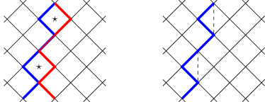
Let us consider an isolated cluster of blocks. For simplicity we consider a cluster with trivial topology like that shown in Fig. 5, but a general cluster with holes inside can be treated similarly. Eq. 44 shows that the weight of the spin configuration vanishes if any block has two spins of the same sign ( or ) above it, so the cluster must lie on a domain wall between and . We wish to compute the mean square weight of the cluster, .
Haar-averaging maps to a partition sum for spins . The permutations are now in rather than because squaring the diagram doubles the number of layers in the replicated circuit. The spins outside the cluster are fixed, so simply provide a boundary condition for those inside.
This partition sum can be computed relatively simply when is large. We summarize the main features here and give a detailed analysis in App. A.3. The domain wall labelling convention we use is described in Ref. zhou2019emergent : a domain wall with a domain of to its left, and a domain of to its right, is labelled by the permutation .
If we Haar-average the circuit we obtain spins with the interactions specified in Eq. 14. Here the interactions are modified, because we fixed the configurations of spins before squaring and averaging. This involves insertions of , and that modify the triangle weights discussed in Sec. II.2.
In the doubled problem there is a doubled domain wall incoming at the entanglement cut, as illustrated in Fig. 5. In a domain the spins are fixed to , and in a domain they are fixed to . Inside the cluster the spins must be summed over. However, they are very restricted. Because of the modified triangle weights, spin values in the subgroup are suppressed in the interior of the cluster: a triangle whose vertices are all equal and take one of the values , , or has weight zero. In fact we have
| (54) |
where the symbol on the left denotes the weight for a triangle whose lower spin is associated with a block.
In the large limit, the leading term involves the incoming doubled domain wall splitting at the top of the cluster into a pair of doubled domain walls, according to the allowed multiplication (cf. Sec. VI B of zhou2019emergent ):
| (55) |
One doubled domain wall, say , travels along the left boundary of the cluster, and the other along the right. [Since commutes with , either of the two doubled domain walls can be on the left.] In the interior of the cluster, the spin value is then [or ]. This does not incur any “bulk” cost, because a triangle all of whose vertices are equal to has weight unity by Eq. 54.
The two doubled domain walls along the two boundaries of the cluster incur a weight per time step.222At large , an “elementary” domain wall, i.e. a transposition, costs per time step. Here we have a total of 4 elementary domain walls (the right-hand side of Eq. 55). Consequently the mean squared cluster weight is of order or even smaller, where is the time duration of the cluster. (We have not included the cost of the “thin” domain wall sections above and below the cluster.) This indicates a typical magnitude
| (56) |
for a cluster of a given size in a typical large circuit. Note that this weight is much smaller than the weight of a section of thin domain wall of the same time duration. Similar considerations apply to clusters with more complex topology, i.e. with holes inside.
Therefore, any configuration with a cluster lasting for steps has a weight that is suppressed by at least compared to the leading configurations in the same spacetime region.
It should be noted that clusters are suppressed by a cost in the exponent that scales not with their area in spacetime, but instead with the length of their boundary. This is reminiscent of a domain wall between two different spin states in the ordered phase of the Potts model with states, where bubbles of other spin states can appear on the domain wall cardy2000renormalisation . Here this scaling is a necessary consequence of unitarity. As a result of it, the effect of boundary conditions can be subtle. For example, a boundary condition at that favours may be able to induce a large domain of , because a boundary free energy of order can compensate the additional domain wall cost of order in the bulk. This is not the case for the quantities considered here, however. Indeed, for entanglement growth starting from a product state, the boundary condition favours over .
The results above strongly support the conjectures of the previous section. For example, there we defined weights for “steps” of variable temporal duration that connect locations where a domain wall between and is “thin”. We conjectured that the contribution of long steps to the partition function was suppressed. The calculation above confirms this conjecture explicitly for a typical circuit realization at large . (A realization of a random circuit is not translation-invariant, but generalizes directly to this case.) We find that the contribution of long steps to the line tension is suppressed exponentially () in the step duration . Note that, according to our definition in Sec. II.4, a step of duration does not need to include blocks: for example, we can have step with a single block at the top, which allows the domain wall to branch into three domain walls between and , which merge again at the bottom of the step. Such configurations are also exponentially suppressed, simply because they contain extra domain walls, each contributing an factor to the cost zhou2019emergent .
Our results in Sec. V for translation-invariant Floquet spin-1/2 circuits will also be compatible with exponential suppression of large steps (App. B.5).
The results in this Section also mean that, at large , we can obtain the nontrivial fluctuations of the entanglement entropy in a random circuit by considering only single- clusters. We discuss this next, before moving on to deterministic models.
III.2 KPZ/DPRM scaling in the random circuit
Recall that with the appropriate (free) lower boundary condition. Averaging over Haar-random gates gives (Sec. II). However, the averaged Rényi entanglement entropy cannot be obtained from , because of fluctuations.
Let us first recall the replica approach used previously. This involves computing the replicated partition function, , and extracting quantities like from the limit. At large there is a simple picture for the replicated partition function . It describes domain walls that interact via a mutual attraction. In the microscopic spin model, the attraction is due to an additional local spin configuration that is possible when two domain walls come into contact with each other zhou2019emergent .
This description can be identified with the replica description of a well-known classical problem, the directed polymer in a random medium HuseHenleyFisherRespond ; kardar_dynamic_1986 . In that context, the free energy of the polymer can be calculated by replicating the system times and integrating out the disorder. For an appropriate choice of lattice model, the resulting polymers will have exactly the same mutually attractive interactions as the domain walls here. Therefore, we have indirectly mapped the entanglement to the free energy of a single domain wall in a random potential that modifies the weights of steps. This leads to KPZ scaling HuseHenleyFisherRespond ; kardar_dynamic_1986 for the fluctuations of the entanglement.
In the present approach we consider a single domain wall, without replicas. However, to go beyond , we must “dress” the domain wall with insertions of . We have shown above that clusters of are exponentially suppressed in their size. At large it suffices to consider only dilute, isolated clusters made up of a single block. Further, at large the local configuration labelled in Eq. 45 dominates over the other configurations in Eq. 45 (App. A.5).
By Eq. 44, these insertions are restricted to lie on the domain wall. In the notation of Sec. II.4, this gives us a nonzero weight
| (57) |
for a step with and . The notation indicates that this weight depends on the local gate , unlike the deterministic weights . Since all the s are independent, this yields an uncorrelated random potential for our “polymer” in spacetime.333In more detail: since the weight can be either positive or negative, it is convenient to absorb it as a correction to the weight of a pair of length-1 steps. This yields a directed path made of length-1 steps, with a random potential associated with pairs of sites vertically above each other: see Fig. 6, Right. The Boltzmann weight is positive in this representation zhou2019emergent . In an equivalent stochastic differential equation representation for , which is the KPZ equation, determines spatiotemporal noise.
The above picture, with random weights assigned to vertical steps, agrees with the replica approach: we just need to check the strength of the noise matches.
The average vanishes. Its variance is given by the squared average of in Eq. 45 (App. A.5):
| (58) |
where was defined in (26). This matches the result for the variance in Ref. zhou2019emergent .
We therefore confirm that a thin domain wall with dilute insertions reproduces the result of the replica calculation.
IV Floquet spin-1/2 chains: preliminaries
We now apply the formalism of Sec. II to models that are invariant under both space and time translations. In the brickwork circuit geometry, such a model is defined by a single 2-site unitary .
In Sec. II.4 we defined the “thick” domain wall that appears in the calculation of . This reduces this partition function to one for a directed path with irreducible step weights that take into account successively larger clusters of . The line tension of this path can be extracted easily from the weights .
In Sec. V we will present numerical data for several models using this scheme. In preparation for this we next describe how to obtain systematic approximations to and the butterfly velocity from the weights (Sec. IV.1).
The numerical method for obtaining the weights themselves is described in App. B.1. We use exact diagonalization, which allows us to treat up to . Together with the analytical results below, this yields a straightforward algorithm which can be applied to any circuit. Sec. VIII gives an extension to dynamics that are not of circuit form.
IV.1 Extracting from
Recall that the line tension function is encoded in the asymptotics of the partition function defined in Eq. 40:
| (59) |
We use generating functions to determine . Define generating functions for the partition function and for the irreducible weights ,
| (60) | ||||
| (61) |
(The variable in this section should not be confused with the spin variables elsewhere in the paper.) We can relate these generating functions using Eq. 40, which yields a geometric sum for :
| (62) |
By truncating the sum in Eq. 61 at order we will obtain a polynomial approximation to . This approximation is physically motivated: it amounts to setting a maximum step length in the directed walk of Eq. 40. We expect this approximation to improve systematically with for chaotic models.
We then need the prescription for obtaining the asymptotics of , or in other words the line tension , from the numerically accessible quantity . This can be done with the pole method. For a given , let be the smallest root (in absolute value) of the denominator in Eq. 62. Then the desired relation is
| (63) |
This relation is explained in Appendix C. The root appearing here has a physical meaning (although we will not need it here): if we write
| (64) |
then , which is related to by a Legendre transformation, Eq. 63, is the Rényi entropy growth rate in a state with jonay_coarse-grained_2018 .
As an example, consider the lowest-order approximation where we truncate at , corresponding to the partition function without any blocks. We then need only
| (65) |
At this order, , giving the root
| (66) |
The quantity in Eq. 63 is maximized by . Plugging this in gives
| (67) |
This is indeed the correct result for jonay_coarse-grained_2018 ; zhou2019emergent (and also the leading order result in the random circuit at large ).
In the numerical algorithm we compute up to and neglect for larger times. Given a constant , we then solve numerically for the smallest zero of
| (68) |
If we define444 here is real by definition. In principle the smallest root may be complex (in which case it has a complex conjugate partner ). We have allowed for this above. However from the physical interpretation of the quantities above we expect that is real and positive at least for large .
| (69) |
then is given by . (We see this by setting the -derivative of the argument in Eq. 63 to zero, and extracting the derivative of from Eq. 68.) We iterate over to construct the entire curve.
This approach also allows us to extract the butterfly speed , as the point555 If is not reflection-symmetric, there are separate left and right butterfly velocities and jonay_coarse-grained_2018 ; stahl2018asymmetric ; zhang2019asymmetric . In this situation , and , and . Our convention here is that the support of the operator grows, with , to the left at speed and to the right at . where . The “entanglement speed” for the second Rényi entropy, for a quench from the product state, is simply .
It is worth noting that this generating function approach sums up an infinite number of domain wall configurations directly in the thermodynamic limit, eliminating a significant source of finite- effects. As an illustration, if (hypothetically) steps of size greater than had zero weight, the present approach would give the exact result for already at time . In reality the weights are not zero for large , but the analytical results in Sec. III.1 suggest that the convergence in is typically exponential.
By contrast, attempting to directly extract the exponential decay rate of by a fit for is subject to finite- effects that are generically only polynomially small in (as one can see in the case where the domain wall is a simple random walk). Therefore understanding the domain wall structure improves the computation of the line tension.
Ref. jonay_coarse-grained_2018 extracted the line tension associated with the von Neumann entropy for a chaotic Ising model directly from the operator entanglement of . That study indeed noted larger finite– effects than those found here. However, we do not address the von Neumann entropy (as opposed to the higher Rényi entropies) here.
IV.2 General parameterization
In our discussion of the numerical results, it will sometimes be useful to use the following parameterization of the two-site gate , which is an arbitrary matrix kraus2001optimal ; bertini2019exact ; khaneja_cartan_2000 ; piroli_exact_2019 :
| (70) |
where
| (71) | ||||
| (72) |
The s scramble the individual sites and the two-site unitary entangles the two sites.
We will mostly restrict to the reflection-symmetric case such that and . Additionally, is unchanged by the transformation , where is any single site unitary. This amounts to a trivial redefinition of the circuit, and one may check that the conjugate operators and all cancel out in the weights in the partition function. Exploiting this symmetry, we can take
| (73) |
so that the general symmetric gate is parameterized only by the two vectors and .
V Application to Floquet circuits
We are finally ready to apply the numerical scheme in Sec. IV.1 to a variety of Floquet circuit models, described in the following subsections. In Sec. VIII we will show that the restriction to circuits is not necessary. But circuits are especially convenient for numerics since they have a strict lightcone structure (propagation of information outside the lightcone is not only exponentially suppressed, as in generic spin chains lieb_robinson , but exactly zero). The space of circuit models is also already very rich.
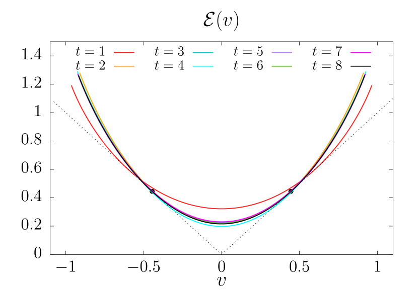
For each model we study we will show the sequence of approximations to , indexed by with : see for example Fig. 7. These successive approximations take weights for longer and longer steps into account.
The curve for (in red) is independent of the gate defining the circuit: this lowest approximation matches the result of the random average computed in Eq. 67. It can be thought of as a baseline showing how far the Rényi entropy growth in a particular circuit deviates from the random average.
Our algorithm works if the curve converges sufficiently rapidly to the actual line tension function. In addition to showing the bare plots, we perform several other checks of convergence. In Sec. V.3 we will directly examine the decay of and at large . The assumption on the structure of the domain wall implies that the latter should be negligible at large .
Additionally, we check that the line tension function satisfies several constraints. It is positive, convex, greater than or equal to , and tangent to this line only at . We therefore plot the boundary curve with dotted lines. We also mark an estimate of from an independent numerical computation of the OTOC (the protocol is described in App. B.3). We show this estimate as a pair of black dots.
Convergence to a form consistent with these constraints is a nontrivial test, because they are not built into the formulas for finite (indeed we will see that they can be disobeyed by the small– approximations).
V.1 Generic symmetric and asymmetric gates
First, we consider the following one-parameter family of reflection-symmetric gates (see Eqs. 70–73):
| (74) |
The parameter tunes the strength of the interaction between the two qubits. For small , local scrambling will take a long time: we do not expect our algorithm to converge rapidly in that case, so we will choose reasonably large. Otherwise, the numbers above are arbitrary and were chosen to ensure (1) that there is no fine-tuning in the sense of any of the coefficients vanishing, (2) that represents a rotation on the Bloch sphere by a significant angle (here ).
Fig. 7 shows results for the gate with . The results are consistent with a relatively fast convergence of . We see that this chosen gate has a smaller and a smaller than the annealed average for the random circuit.
Note that the results are in striking agreement with the general constraints listed above: the asymptotic is a convex curve that touches the line at a single point, which is consistent with as obtained from an independent calculation of .
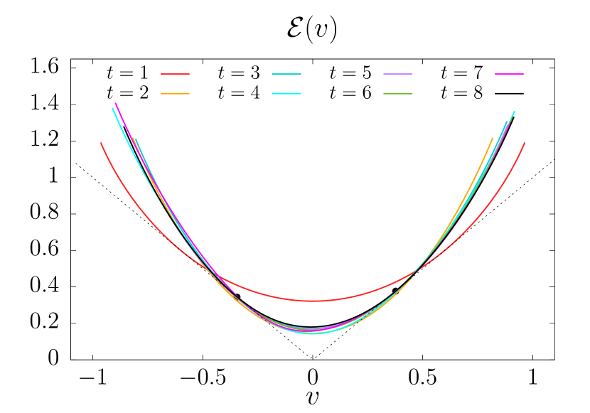
Next, Fig. 7 shows an example of a generic gate without the reflection-symmetry constraint. We simply picked a random gate from the Haar distribution on and used it to build a translation-invariant circuit. The matrix elements of this gate are given explicitly in Appendix 164.
Again, the algorithm appears to be working. However the convergence is now to an asymmetric curve with . The touching point on the left marks and that on the right marks .
V.2 Chaotic Ising models
Next we consider Floquet “kicked” Ising models prosen_chaos_2007 ; kim2013ballistic ; kim_testing_2014 with the Floquet unitary
| (75) |
with a longitudinal field to spoil integrability:
| (76) |
This can be written in the brickwork circuit form (Fig. 3) with the gate
| (77) |
where:
| (78) | ||||
| (79) |
We expect that for generic values of the parameters this gate defines a chaotic model. In special limits, such as or , the model becomes integrable: in those limits we do not expect our algorithm to succeed.
Interestingly, this model also has a “self-dual” line in parameter space akila_particle-time_2016-2 ; bertini_exact_2018 ; bertini_entanglement_2018 ; gopalakrishnan_unitary_2019 ; bertini2019exact ; piroli_exact_2019 :
| (80) |
where some quantities can be computed exactly. In particular, entanglement growth is maximal on this line. This is related to the fact that for this choice of parameters, the tensor remains unitary if it is rotated so as to exchange the roles of space and time gopalakrishnan_unitary_2019 ; bertini2019exact ; piroli_exact_2019 . This has been referred to as “dual unitarity”. Though this property is highly fine-tuned, the model is believed to remain chaotic for generic values of on this line bertini_exact_2018 ; piroli_exact_2019 .
The fact that for the dual-unitary models implies and that the line tension is flat as a function of velocity jonay_coarse-grained_2018 :
| (81) |
This is an interesting test case for our algorithm. First, the above form is very far from our perturbative starting point. Second, the flatness of implies that for dual-unitary models the large-scale properties of the domain wall are rather different from the generic case, with negative signs in playing an important role. We describe this in Sec. VI.
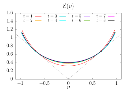
To begin with we check the algorithm for a presumably generic set of parameters within the kicked Ising class in Fig. 8:
| (82) |
The algorithm appears to be working, and the curves converging to one that represents a gate more entangling than the random average.
Kim and Huse studied similar values of the fields,666More precisely and . Here we have used the truncated decimal values. but with the smaller period kim_testing_2014 . However, the Kim–Huse values happen to be quite close to the dual-unitary values777Writing the gate with in the representation in Eq. 70 gives . One branch of dual-unitary values is with any and any ., which are ! This explains the strong entanglement growth in the Kim-Huse model. Our numerical results for this case (not shown) give a line tension function with a close to 1 and a larger than for .
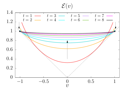
We now check our algorithm for the dual-unitary case, taking888In terms of the general parameterization in Eq. 70 bertini_exact_2018 ; bertini_entanglement_2018 ; gopalakrishnan_unitary_2019 ; bertini2019exact ; piroli_exact_2019 , , , and .
| (83) |
The value of is not important for the dual-unitarity condition, but we should have to avoid the model being free. Empirically we only see very small differences for the line tension function among different choices of , including the special point where the dynamics is Clifford as well as being dual-unitary.
Results are shown in Fig. 8. The curves seem to converge to the expected flat line . The touching points where seem to converge to the expected value very fast.
Therefore the domain wall structure appears to make sense even for dual-unitary gates, which represent a limiting case. However in this case negative signs in are important: without these it is impossible to have a flat , see Sec. VI.
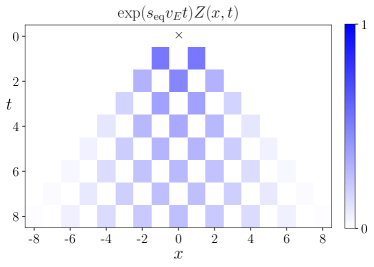
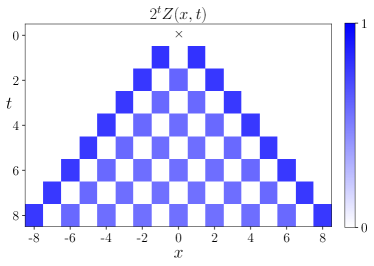
V.3 Structure of matrix
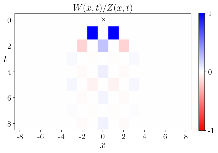
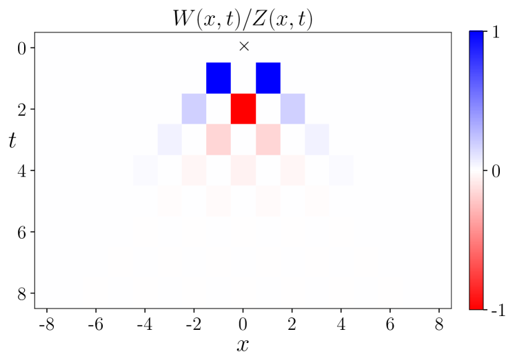
We now examine the temporal decay of the step weights defined in Sec. II.4. In order to examine the importance of long steps, we consider the normalized quantity : this compares the weight of a single long step, with displacement and duration , with the total weight of all paths with the same two endpoints. This ratio should decay with if asymptotically long steps can be neglected. (Individually, both and decay exponentially with .) A slight extension of the reasoning in Sec. III.1 shows that in a typical realization of a random circuit at large , the typical value of this ratio (for a given starting point of the domain wall in spacetime) decays like .
Fig. 9 shows heat maps of for examples of translation-invariant Floquet models for spin-1/2s. Panel (a) is for the generic reflection-symmetric gate in Eq. 73, whose line tension function was shown in Fig. 7, and Panel (b) shows the dual-unitary gate of Eq. 83 and Fig. 8.
In both cases the weight is small at large , though finite-time effects in this quantity seem to be large for the former gate at displacement . We also find decay of for the generic asymmetric gate discussed in Sec. V.1 and for the kicked Ising model with the generic parameters in Eq. 82 (data not shown).
The domain wall picture appears to be well-defined both for the generic models and for the dual-unitary model. However there are key differences between the two cases which we discuss in Sec. VI. Note that the weight at , is positive for the gate in Panel (a) and negative for the dual-unitary gate in Panel (b). In the former case this extra positive step weight increases compared to , leading to decreased . In the latter case the negative step weight decreases compared to , helping the dual-unitary gate to attain the fastest possible decay of , i.e. the most rapid possible entropy growth.
Let us also show an example where local gate is very weakly entangling, resulting in slower convergence of the algorithm. This is the reflection-symmetric gate defined in Eq. 74, but with the smaller interaction constant (in Sec. V.1 we showed results for ).
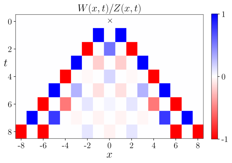
First we show the ratio in Fig. 10. We see that there are large values close to the edges of the lightcone. However, the apparent decay inside the lightcone suggests that the results may still converge, just more slowly than in the cases examined above.
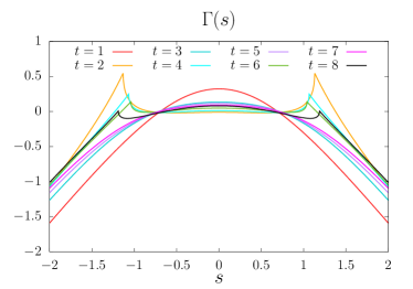
The slow convergence in this case is related to the fact that the gate is weakly entangling. First we examine the function defined in Sec. IV.1 (whose physical meaning, for , is as an entanglement entropy growth rate in a state with a nonzero gradient in the entanglement across a cut at position , with ). The approximations to for are shown in Fig. 11. Note that they are no longer concave functions over the whole range . However, this effect gets less severe with increasing . If we restrict to the concave region in performing the Legendre transform, we get a reasonable result for : see Fig. 11. This is consistent with slow convergence to a function that satisfies the general constraints, with a very small entanglement growth rate.
For a quantitative analysis of convergence rates in the various models, See App. B.5.
VI Coarse-graining: generic models versus dual-unitary circuits
The thin domain wall conjecture implies that the entanglement membrane is well-defined once we coarse-grain sufficiently in space and time. The relevant lengthscale, the width of the domain wall, is microscopic, in the sense that it remains finite as the system size and the total time of the evolution go to infinity. In the models investigated here, which do not contain any small parameter, the width of the domain wall is an order 1 multiple of the lattice spacing. In cases where the dynamics is tuned close to a special point, a large lengthscale may emerge.
In this section we discuss this coarse-graining in slightly more detail, in order to make a distinction between two universality classes.
Microscopically, the step weights can be of either sign. But we conjecture that, for generic models, the minus signs do not alter the universality class from that of a classical directed path. Heuristically, we can think of the step weights becoming positive after coarse-graining, so that the membrane is effectively a classical directed path with diffusive wandering (at least for ). We will restate this in terms of the recursion relation for below.
This coarse-grained picture implies a strictly convex , with a positive second derivative that is related to the diffusivity of the path. [This diffusivity can depend on the coarse-grained velocity that we condition on.] This implies for example that the scaling of is:
| (84) |
The power-law prefactor is universal and comes from the fact that both endpoints of the random path are fixed. For example, consider the case where , so that the coarse-grained velocity is close to zero, and let the model be parity-symmetric. Expanding in , the above is then
| (85) |
where we have factored out the extensive free energy of the path by defining (recall )
| (86) |
Up to a normalization constant, Eq. 85 is the probability for a random walker with diffusion coefficient
| (87) |
to be at position at time . In Fig. 12 we show for a generic kicked Ising gate: these numerical results are in good agreement with the scaling in Eq. 85 (App. B.6).
The dual-unitary model behaves differently. The membrane and its line tension function still appear to make sense, but its wandering is not diffusive. For example, we can contrast the scaling of with the formula above. The numerical results in Fig. VI.1 are consistent with the large scaling
| (88) |
with a trivial -dependence inside the lightcone (we neglect the even-odd effect at the lattice scale). This is also consistent with the analytical calculation in Sec. VI.1 below.
Evidently, in the dual-unitary case, the membrane is not a classical random walk. Indeed, since for the dual-unitary model is constant (inside the lightcone) and vanishes, the diffusivity in Eq. 87 must diverge in the limit that a model becomes dual unitary.
The distinction between the two cases may be clearer if we think of the recursion relation as a discrete analogue of a linear partial differential equation. In the limit of large , we may write Eq. 43 as
| (89) |
We would like to relate this to a continuum equation in the limit of large times. We cannot immediately perform a derivative expansion of : since it is exponentially decaying, higher derivatives are not parametrically smaller than lower ones. For simplicity, consider first the regime discussed above (close to the ray) and assume reflection symmetry (so ). Then in Eq. 86 has a sensible derivative expansion. Let us define the following “average” for an arbitrary function ,
| (90) |
(We have replaced , with , to avoid clutter. The subscript on the average specifies the spacetime ray whose vicinity we are considering.) This satisfies , by the relations in Sec. IV.1. The derivative expansion of Eq. 89 yields:
| (91) |
plus less-relevant terms. The thin domain wall assumption implies that the two coefficients shown are finite. While the weights defining the averages are not necessarily positive, the averages shown will be nonzero in the absence of fine-tuning. The higher terms can then be dropped, leading to the diffusive (random walk) scaling discussed above. We can also check using the relations between generating functions that
| (92) |
so that the diffusion constant in Eq. 91 agrees with that in Eq. 84. We emphasize that the above equation is valid only close to the ray: see below for a more general equation. The information contained in Eq. 91 is already contained in , and the spacetime picture is usually more convenient.
The universality class changes if vanishes due to fine tuning. It is clear from the definition in Eq. 90 that this requires negative step weights (which are absent in the large limit described in Sec. III). When this vanishing occurs, we must take into account the next time derivative term, which was previously irrelevant:
| (93) |
This is what occurs in the dual unitary model above. We see that the equation becomes a wave equation, consistent with the constancy of inside the lightcone (Sec. VI.1). We checked that is consistent with zero in the dual unitary circuit: the finite approximation to from the truncated matrix decays exponentially in , with a characteristic time steps.
To simplify further, let us consider a toy model, which only takes a single additional nonzero element (beyond the ones present in ). We parameterize its elements in terms of a constant
| (94) |
When we are in the diffusive class. However when (in fact the dual unitary model is numerically quite close to this simplified model), removing the factors of by defining gives
| (95) |
which is a discrete version of the wave equation, . This gives a which is constant inside the lightcone and zero outside.
Numerically, we find that the structure in the specific dual unitary kicked Ising model that we studied above is similar: is approximately constant within the lightcone, and zero outside. Fig. 12 contrasts the spacetime pattern of for the generic kicked-Ising model and the dual-unitary kicked Ising model.
In the derivations of the continuum equations (Eqs. 91, 93), we restricted to the vicinity of a particular ray. For a more general equation, we may write , and expand in derivatives of . The resulting dynamical equation jonay_coarse-grained_2018 also applies to the second Renyi entropy of a time-evolving quantum state in a 1D system, for an entanglement cut at .999This corresponds to a different lower boundary condition, where the domain wall endpoint at is free and weighted with . The recursion relation is the same. As described in Eq. D, this gives the equation
| (96) |
where is the Legendre transform of (Sec. IV.1). The first term is the leading-order dynamics that captures the term in the entanglement. Here and are generally of order 1 at late times, so we keep all powers of , but higher derivatives are small and we can expand in them. The second term gives subleading corrections jonay_coarse-grained_2018 . The random walk picture implies that the two coefficients are related. The above equation can also be written in terms of , giving a form consistent with Eqs. 92, 91 (App. D).
VI.1 Partition function for dual unitary models
Let us confirm by an explicit calculation that dual-unitarity implies the abovementioned approximate constancy of within the lightcone [which is related to the wavelike structure of the recursion equation for , and which implies constancy of as a function of ].
This fact can be seen by considering a slightly different partition function, in which we place states at the lower boundary, rather than the dual states used in Eq. 35:
| (97) |
Here and label the positions of the domain walls between and on the top and bottom boundaries respectively. Fig. 13 shows an example of . In contrast to the domain wall partition function defined in Eq. 35, does not force the end point of the domain wall to lie precisely at , but instead penalizes configurations whose end point deviates from (with a negative power of in the weight). However, in analogy to the random circuit case, we expect that this difference only leads to an boundary term in the free energy (so long as , which in the dual-unitary circuit is a trivial restriction since ), so that
| (98) |
Physically, the above partition function simply computes the operator entanglement of the time evolution operator itself, for a certain partition of the “legs” of the time evolution operator. This operator entanglement is maximal in the dual unitary circuits, like various other measures of entanglement in these systems bertini_exact_2018 ; gopalakrishnan_unitary_2019 ; bertini2019operator ; piroli_exact_2019 . This is easily seen by manipulations similar to those in gopalakrishnan_unitary_2019 ; bertini2019exact ; piroli_exact_2019 . Specifically (setting ) we show that for a dual-unitary circuit, so long as is within the light cone of the origin.
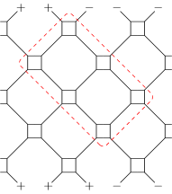
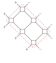
We represent the multi-layer two-site unitary evolution matrix as a four-leg tensor:
| (99) |
We have labelled the external legs of this tensor by . As a unitary, the legs correspond to the row index and to the column index. We rotate the tensor by to obtain the dual tensor. Dual-unitarity requires the dual tensor to be unitary (with as row legs and as column legs) as well. To contrast with the generic gate in Eq. 47, we have drawn the dual-unitary tensor as a (fourfold symmetric) square in Eq. 99. For , unitarity and dual-unitarity can be used to propagate (or ) states from the top to bottom, right to left, and vice versa. Graphically, we have (the same holds for arbitrary with replaced by any )
| (100) |
The first of these relations (unitarity) allows us to remove the unitary gates outside the lightcones in Fig. 13. Keeping track of the factor, equals the expression in Fig. 13. Next, dual-unitarity (the second relation) can be used to propagate the states to the right, so that all the unitary gates are removed and Fig. 13 is reduced to . Hence , so that within the lightcone.
VII Operator spreading
We have focused on the second Rényi entropy as a test case, but the present formalism can be applied to almost any observable expressible in terms of . One of the simplest is the out-of-time order correlation function, which requires , and which on large scales we expect to reduce to a stochastic growth process nahum_operator_2017 ; von_keyserlingk_operator_2017 .
The OTOC can be written in terms of the same partition sum as for , but with different boundary conditions. In the Haar-averaged circuit this reduces to a simple partition function for a pair of domain walls. Since we have now made sense of the domain wall in a generic, fixed circuit, this picture from the random circuit carries over. The modification is that the domain walls now have a nontrivial internal structure, including finite regions of , with an associated microscopic timescale . A typical configuration from the partition sum is illustrated in Fig. 14.
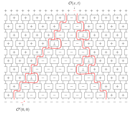
For a brief heuristic summary, we consider the OTOC in the form of a commutator squared of two traceless operators,
| (101) |
We take the expectation value at infinite temperature, and to simplify the boundary conditions we average over local unitary rotations of the local operators , . Carrying out manipulations similar to Sec. VI B of nahum_operator_2017 , we rewrite using the present notation (here is a single-site trace)
| (102) | ||||
The operator insertion at the top initiates a domain of in the bulk. Because of the boundary condition at the bottom, this domain prefers to expand at rate (assuming reflection symmetry).101010The lower boundary condition contributes a weight proportional to , which tries to increase the width of the domain at the lower boundary. The boundary weight means that the optimal velocity for the left domain wall, minimizing the free energy, is , since by the properties of this minimizes .
However, the operator insertion at the initial time cannot lie in the region exterior to the domain, because this would lead to a factor of . If then is constant at leading order, . But if , the lower operator insertion “stretches” one of the domain walls, forcing it to move at a speed greater than . This is illustrated for the left domain wall in Fig. 14. The additional free energy cost means that, outside the lightcone, for , the OTOC scales as khemani_velocity-dependent_2018
| (103) |
In random models these results can also be obtained from a stochastic growth process for the operator cluster von_keyserlingk_operator_2017 ; nahum_operator_2017 ; rowlands2018noisy . In this picture, is the large deviation function describing the probability for the boundary of the operator cluster to propagate at speed correlatorpaper . From the above discussion, we expect that in generic models this stochastic picture applies after coarse-graining to timescales greater than .
Forthcoming work using the memory matrix formalism will give a complementary view on the operator spreading problem mccullochforthcoming .
VIII Beyond circuit models
In Sec. II we described how to introduce the pairing field (the spin in the effective partition function) in the context of models with a circuit structure. This was a natural starting point, since the idea of inserting permutation states was inspired by the random unitary circuit. However there is no need to restrict to circuits.
In this section we study generic Floquet systems, i.e. models where the Hamiltonian is periodic in time, but which do not have the form of a circuit. We are still free to insert resolutions of identity as in Eq. 11:
| (104) |
In this graphical equation, the shaded region denotes the Floquet operator (evolution operator for one time period), which in general will not have an exact circuit decomposition. As in Eq. 11, the horizontal bars represent projectors onto either a permutation state or the subspace, these possibilities being summed over.
For models that are translationally invariant by 1 lattice spacing, an alternative that may appear at first sight more natural is to insert single-site, rather than two-site projectors:
| (105) |
Both rewritings of are exact. In the following we consider both schemes.
The partition functions are sums over spins , taking values, associated with each horizontal bar. We focus on the case of the purity (), where can be or . We choose a graphical notation that resembles that for the circuit, labelling the shaded region immediately above the horizontal bar with the bar’s spin value: see Fig. 15. This figure shows possible spin configurations for a section of domain wall of finite width in the two schemes.
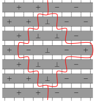
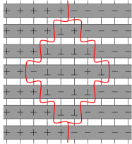
The numerical algorithm in Sec. IV.1 can be carried over with little modification. We first define the partition function the same way as in Eq. 35 — the difference here is that may be nonzero even when is arbitrarily large. We then solve for the irreducible step weights recursively, using Eq. 43.
The approach is feasible because the Floquet evolution has an emergent Lieb-Robinson light cone lieb_finite_1972 which suppresses for large . For practical computation of , we must truncate the Floquet operator to a chain of finite length , so at the end we must check that our results are converged in . For a fixed , the error introduced due to the finiteness of should be exponentially small at large , but of course the required grows linearly with .
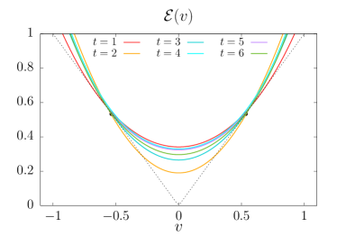
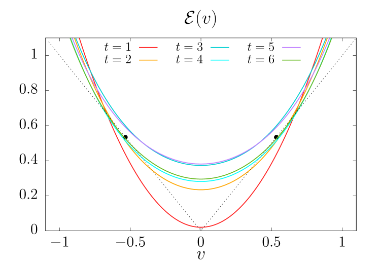
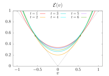
We consider two examples of an Ising model with an oscillating transverse field ,
| (106) |
In the first example is a square wave with period , taking the values and for half the period each:
| (107) | ||||||
The Floquet operator is then
| (108) |
with equal to (106) with the appropriate value of .
In the second example oscillates sinusoidally, with period ,
| (109) |
the parameters , and being the same as in Eq. 107. Neither of these two examples allows a circuit representation.
For the first system (square wave) we compare the 1 and 2 site insertion schemes. Fig. 16 shows approximations to the line tension function, for increasing values of , in a system of spins, for the two-site and one-site schemes respectively. We position the domain wall at the top boundary so as to minimize finite– effects, see the numerical details in App. B.1. (Performing calculations for a given with multiple choices of the top boundary condition incurs an additional cost, but this is a subleading factor.) We compute up to . We estimate the error due to the finiteness of by computing the difference in the result for for and for . We find a relative error for the two-site scheme and for the one-site scheme.
For both schemes, the curves in Fig. 16 are consistent with reasonable convergence to a legitimate line tension function, with a value of consistent with that computed directly from the OTOC.
One counter-intuitive feature of Fig. 16 is that the two-site scheme performs better than the one-site scheme for small (the one-site scheme is also more expensive computationally). The contrast is most obvious at , where the curve for the one-site scheme (Fig. 16) strongly violates the constraints of the line tension. Despite this, the two curves for are in remarkably good agreement, with relative difference in the entanglement velocity estimates.
IX Outlook
In random circuits, the “pairing field” and the membrane picture emerge in a simple way from the average over unitaries whenever we deal with dynamical quantities that require multiple forward and backward evolution operators (such as Rényi entropies or OTOCs). Here we have shown how to make sense of the pairing field, which describes a pairing of trajectories in the multi-sheeted path integral, in realistic systems that do not involve randomness. This opens the way to extending the various results that have been obtained in random circuits to a much broader class of more realistic models. More generally, by identifying appropriate effective fields, it provides a framework for applying the renormalization group to chaotic real-time dynamics.
We separated the local multi-copy Hilbert space into “paired” states, and states in their orthogonal complement, . Dynamical quantities then became partition functions for an effective field . The state of the effective spin here is reminiscent of the state , representing a vacancy, in the Blume-Capel model (the classical Ising model with vacancies, where the spin takes the values ). We have shown that in strongly chaotic Floquet systems the “vacancies” dress the structure of domain walls between different pairing states, but leave the basic structure of the domain wall intact on large scales.
After using a typical realization of a random circuit as a test case, we applied this picture to Floquet systems, for spin-1/2, that have no small parameter at all and no randomness.
The method gave convincing results for the line tension function for (which determines both the second Rényi entropy growth rate and the butterfly velocity) from calculations on relatively small lengthscales. A simple but important ingredient was a resummation of the weights in the spin model into a single function , describing the amplitude for the membrane — which in 1+1D can be viewed as a directed path — to take a step of temporal extent and spatial displacement . Interestingly, there was a qualitative difference in the structure of for generic Floquet models (whether circuits or not) and for dual-unitary, maximally entangling circuits.
Many questions remain for the future. First, there are many kinds of extra structure that could be incorporated and which might be expected to have interesting effects.
We have focused on Floquet models without any conserved quantities. Any slow mode, for example a conserved charge, will interact with the dynamics of the membrane. (A single physical conserved charge gives rise to multiple conserved charges in the replicated Hilbert space.) Results on random circuits with conservation laws provide a starting point rakovszky_diffusive_2017 ; khemani_operator_2017 . Our approach can be extended to models with conservation laws by refining the resolution of the identity to specify information about the charge as well as the permutation: we will discuss this elsewhere. One cautionary note is that it has recently been shown that the dynamics of the higher Rényi entropies, for which the present method is suitable, can be qualitatively different from the that of the von Neumann entropy in models with conservation laws rakovszky_sub-ballistic_2019 ; huang_dynamics_2019 ; zhou2019diffusive ; znidaric_entanglement_2019 .
In the present approach, the von Neumann entropy corresponds to a nontrivial replica-like limit, which it would be interesting to understand better even in the absence of conserved quantities.
Also interesting are continuous spatiotemporal, as opposed to internal, symmetries, for example Lorentz invariance. Such symmetries will constrain the effective field theory of the membrane, as well as giving new hydrodynamic modes liu_lectures_2018 ; rangamani_gravity_2009 .
There is considerable freedom in the precise way in which the effective spins are introduced. We focused mainly on inserting a resolution of the identity for pairs of sites, since this was convenient for making contact with the Haar-random circuits studied previously. We also explored the use of single-site resolutions of the identity: this appeared to be less efficient for the model we studied. It would be useful to understand this better in order to optimize the efficiency of the scheme.
The basic idea of this paper is not restricted to 1+1D: the effective partition function can be introduced in the same way in any number of dimensions, and we may again argue for the coarse-grained picture in terms of a codimension-1 membrane dressed with states. However, the additional computational cost means that in higher dimensions we are likely to need either special structure, or a small parameter, in order to obtain quantitative results. The method may also be applied to dynamics without spatial structure, in which any qubit can interact with any other.
For the observables studied here, the pairing between layers of the circuit is local in time. For some dynamical quantities, for example the spectral form factor, pairings that are non-local in time play a role chan_solution_2018 ; chan2018spectral ; kos2017many . It would be interesting to extend the present approach to this setting.
Our method for defining the effective spin model might illuminate other interesting universal dynamical phenomena. First, we may consider how the description in terms of an entanglement membrane breaks down on approaching a many-body-localized phase. We hope to return to this elsewhere. There are other failure modes that could be investigated, for example the approach to a noninteracting or integrable point.
Within the more limited domain of random circuits, the effective spin model here may also give a way of thinking about entanglement in random Clifford circuits which is more generalizable (e.g. to higher dimensions) than the approach of mapping the evolution of stabilizers to an effective classical stochastic dynamics nahum_quantum_2017 ; li2019measurement ; gullans2019dynamical .
The approach could also be used to study questions motivated by quantum information such as the emergence of the “design” property in random circuits with non-Haar–distributed gates harrow2009random ; brandao2016local ; roberts2017chaos ; cotler2017chaos ; hunter-jones_unitary_2019 .
The effective spin model may also be extended to dynamics with measurement, or other types of interaction with an environment, for example to clarify the relationship between different universality classes of measurement-induced criticality skinner2018measurement ; li2018quantum ; chan2018weak ; choi2019quantum ; szyniszewski2019entanglement ; li2019measurement ; cao2018collective ; gullans2019dynamical ; gullans2019scalable ; tang2019measurement ; bao2019theory ; jian2019measurement ; zabalo2019critical .
The approach could also be adapted to study tensor networks that do not involve a time direction, for example in the context of the AdS-CFT correspondence where random tensor networks have been used hayden2016holographic ; vasseur2018entanglement .
For chaotic dynamics, further numerical tests and further development of the numerical scheme, extending the range of models to which it could be applied usefully, would also be worthwhile and might give new insights into the physics on the scale of the membrane thickness (which, in many natural situations where there is a small parameter at hand, may be much larger than the lattice spacing).
Acknowledgements.
We thank John Chalker, Tibor Rakovszky, and in particular Curt von Keyserlingk for very useful discussions. TZ was supported by a postdoctoral fellowship from the Gordon and Betty Moore Foundation, under the EPiQS initiative, Grant GBMF4304, at the Kavli Institute for Theoretical Physics. This research is supported in part by the National Science Foundation under Grant No. NSF PHY-1748958. We acknowledge support from the Center for Scientific Computing from the CNSI, MRL: an NSF MRSEC (DMR-1720256) and NSF CNS-1725797. AN was supported by a Royal Society University Research Fellowship.Appendix A Properties of the spin model
A.1 Projectors onto permutation states
The operator defined in Eq. 14 is a projection operator onto the permutation state (it is a nonorthogonal projector, i.e. ). Here we prove the projector property in Eq. 16. According to the definition of in terms of the Weingarten function and permutation states in Eq. 14, we have
| (110) |
We have simplified the notation by writing as a shorthand for the two-site state . This emphasizes that the formulas here apply to an arbitrary Hilbert space, using the Weingarten functions for the appropriate value of the Hilbert space dimension (equal to here). We will return to the previous notation after Eq. 113. Note that states associated with distinct permutations are not orthogonal.
Unless , the function , viewed as a matrix with and as its indices, is the inverse of the Gramian matrix gu_moments_2013 ; collins_integration_2006 :
| (111) |
This means the states defined in Eq. 15 indeed form the dual basis,
| (112) |
So for , we have
| (113) |
Any four-layer unitary gate with the projector attached at the bottom is equal to (Eq. 19). In Eq. 18, we represent the projector as a tensor (box) labelled with a inside. Given the expression in Eq. 14, it can be decomposed as
| (114) |
where the ket is the two-site dual state of , and the bras at the bottom just give on the two sites.
This structure helps us to clarify the definition of the triangle weights as the result of contracting the red part of the following tensor:
| (115) | ||||
| (116) |
which yields the expression of in Eq. 23.
A.2 -independence of the weights
The triangle weights
| (117) |
define the interactions of the effective spin models arising from the random untiaries. The spin is an element of , where is the number of copies of and of in the multi-layer circuit.
In some cases of interest to us the spins , , are all in the smaller permutation group , with , corresponding to permutations involving the indices only. For the corresponding bras, the first layers ( “” layers and “” layers) can be paired arbitrarily, with the pairing labelled by a permutation in , and the remaining layers are paired in the manner prescribed by the identity permutation. For example, consider the case and :
| (118) |
This weight is independent of (proved algebraically in zhou2019emergent ). This -independence holds whenever all the spins are in the permutation group , as conjectured in zhou2019emergent and proved by Hunter-Jones in Ref. hunter-jones_unitary_2019 . Here we review this result.
Algebraically, the triangle is the coefficient in the expansion (24):
| (119) |
(the two spins refer to the two spatial states), which is equivalent to the definition in Eq. 23,
| (120) |
as we see by using Eq. 111 to extract a particular coefficient on the right hand side of Eq. 119.
Now consider the case where , where is the subgroup mentioned above.111111By the symmetry in Eq. 30, the following also applies to other subsets of states related to this one by left and right multiplication with fixed elements of . The fact that the resulting weights are independent of is not immediately apparent from Eq. 120, but can be seen from Eq. 24. When , we have
| (121) |
For example, we can see this by writing the projection operator as the average of a stacked random unitary. The unitaries in the layers with index greater than cancel, since the bra contracts them together in the same way on each site. This leaves the average of a stack acting only on the first layers, which is equal to acting on those layers. The identity acts on the remaining layers.
This shows that in Eq. 121 the only nonvanishing terms on the right-hand-side have as well. As a result Eq. 121 becomes equivalent to the same equation for the -layer case (except that both sides are tensored with the “identity” bra for the remaining layers). This shows that the triangle weights are the same as in the -layer case, i.e. independent of .
Note however that if all of the spins are in , where the subgroups refer to the first and the last layers respectively, the weight does not factorize in general. That is, if we have
| (122) |
where and etc., the triangle
| (123) |
is in general not equal to
| (124) |
The two are equal if, for example, .
A.3 Suppression of large clusters
We analyze the spin model that arises in computing the mean square weight of a cluster like that in Fig. 5. (The average is over Haar-random unitaries.) The spins take values in , because in total we need four layers and four layers to write . We will see that there is a distinction between spin values in the subgroup generated by and , and spin values outside this subgroup. At leading order, the former are forbidden inside the cluster.
We first look at the region outside the region. Each block there is labelled either as or , indicating a local insertion of before squaring. Recall that this projection operator “absorbs” the local unitary gate: equivalently, in the squared system a given block is (recall that each acts on two physical sites):
| (125) |
and similarly for . This defines an interaction triangle for the case where the lower spin in the triangle is from a plus block, in analogy to the triangle interaction defined in Sec. II.2 for the case without the factor. However, because of the projection operator, the spin associated with the block (the lower spin of the triangle) is fixed to be . Similarly, the spin associated with a block is fixed to be . Therefore in computing , the spins outside the cluster are not free to fluctuate. Their role is to provide a boundary condition for the spins inside the cluster.
Explicitly, the weights are (from Eq. 24 with replaced by ; the weights are related to the following by symmetry)
| (126) |
Using the expression for the projector in Eq. 27, this triangle is equal to
| (127) |
Since , in the large expansion, the triangle is at most of order
| (128) |
and similarly the triangle can be bounded by
| (129) |
Here and can be understood as the numbers of elementary domain walls (i.e. number of transpositions) on the left edge of the and triangle respectively. And similarly the corresponding terms are for the right edge. We thus interpret Eq. 128 and Eq. 129 as costing per out-going domain wall on the two edges.
Inside the cluster we have blocks. These lead to a “” interaction triangle defined by:
| (130) | ||||
where we have used the equivalence between the parallel projection and the Haar averaged stack of unitaries.
The right-hand-side of Eq. 130 gives the triangle weight as the difference of two terms. The first term is the ordinary triangle weight for . The second term vanishes unless . Depending on whether , the large expansion yields
| (131) |
For the first case, the triangle weight is exactly equal to an ordinary triangle
| (132) |
We again interpret the corresponding expansion (the first line) in Eq. 131 as a cost of for each outgoing elementary domain wall. For the case of , we can show using the large expansion techniques in Ref. zhou2019emergent, that the term of order cancels, which therefore incurs an additional cost of . In particular, if are also in , then the triangle vanishes exactly:
| (133) |
With this in hand, we can estimate the cost of a cluster in Fig. 5. Because of the vanishing weight in Eq. 133, each triangle inside region must host at least one spin that is not in . Therefore in each time slice that contains a there are at least four elementary domain walls. By the estimates above, each costs at least per time step, regardless of whether it is inside the region or on the boundary between the and regions. A cluster that persists for steps is therefore suppressed by a factor of or smaller. This completes the argument in Sec. III.
The cost of is achieved by the following configuration. We set the spins in the cluster to . The triangle weights inside the cluster are then , by Eq. 132. There are two elementary domain walls making up the composite domain wall on the left boundary of the cluster and two elementary domain walls making up on the right boundary. They enter the cluster through the triangle
| (134) |
which is equal to the ordinary triangle and costs . Meanwhile on the boundary, the four domain walls also cost , according to Eq. 128 and Eq. 129. In total, the weight is for the squared average of the cluster.
A.4 Minimal cluster and operator purity
In Eq. 45, we listed four non-trivial configurations for an isolated surrounded by and . Here we compute their weights for a fixed unitary at the location of the . We will see they are related to the operator purity of .
It is more transparent if we represent each and block graphically as in Eq. 114:
| (135) |
The weight on the left-hand-side is equal to the c-number given by contracting the colorful parts of the tensor on the right-hand-side. The 4-leg tensor (red) is . We can rewrite it as . It is contracted with states and on the top (blue) and the kets at the bottom from the green tensors:
| (136) | ||||
Combining these, we have
| (137) | ||||
where the symbols around the block in the second line indicate contraction with (at the top) or (at the bottom). Similarly,
| (138) | ||||
| (139) | ||||
The blocks on the second line, representing different contractions of , are the operator purities for different partitions. Two of them are actually independent of the unitary gate :
| (140) |
This is because and are invariant under the action of . The other two terms are proportional to the operator purity of vertical and diagonal partitions:
| (141) |
Using these operator purities and simplifying, we obtain the expressions in Eq. 49.
A.5 The size of the fluctuations
In Sec. III, we listed four local configurations where an isolated lies at the path of the domain wall. The average weight of each configuration is zero in the Haar ensemble. In this appendix we estimate their fluctuations, i.e. their mean-square values:
| (142) |
by the symmetry under spatial reflection and exchange. We thus evaluate the other three.
The averages of these diagrams generate the model discussed in App. A.3. They can be expressed in terms of and triangles:
| (143) |
where and label the types of the triangles and are determined by the spins in the bottom two blocks of the configurations in Eq. 142. Because of the doubling of layers (due to squaring), corresponds to (e.g.) , and corresponds to . We can write these weights as
| (144) |
where the sum is over the spin at the center vertex and
| (145) | |||
| (146) |
The lower spins of the second and triangles in this product are fixed to be and respectively, so are not written explicitly. According to Eqs. 128 and 129, the and triangles have the leading order expansion
| (147) | ||||
| (148) |
For , we have , and
| (149) |
| (150) |
where Eq. 150 is based on the large expansion in Eq.(60) of Ref. zhou2019emergent .
Hence
| (151) |
On the other hand, if , the triangle is equal to an ordinary triangle (Eq. 132). There will be at least four out-going domain walls in the triangle, and we have
| (152) | ||||
| (153) |
and
| (154) |
So
| (155) |
These inequalities can be saturated only when
| (156) |
Therefore, the largest terms in Eq. 142 are:
| (157) | ||||
| (158) | ||||
| (159) |
In other words, dominates and scales as
| (160) |
Note that we may also write
| (161) |
where we have used to split into , and
| (162) |
We may then use the result for in Sec. VI A of zhou2019emergent .
Appendix B Further details of numerical results
B.1 Protocol to compute and
In the main text we defined the partition function for a domain wall with fixed upper and lower endpoints (fixed by contracting with and states at the top boundary and and states at the bottom, see Eq. 35).
A naïve way to evaluate numerically is by contracting with these boundary states as per its definition. However, it is numerically inefficient to store the full four-copy unitary .
It is much easier to compute modified partition functions whose bottom boundary conditions only contain . We have discussed a subset of these modified partition functions, which we called , in the context of dual-unitary circuits in Sec. 43. We can view the unitary circuit representing the single-copy time evolution operator as a state on spins, and view all the legs with the boundary condition as a subsystem. The modified partition function is then proportional to the operator purity for this partition. By rewriting the states at the bottom boundary via
| (163) | ||||
we find that is a linear combination of these operator purities. Our numerical scheme then computes these operator purities and obtains as the linear combination. We can then recursively compute through Eq. 43. This scheme enables us to compute up to for a circuit.
For general Floquet evolutions that do not have a circuit representation, discussed in Sec. VIII, the exact computation of requires in principle infinitely many operator purities of the Floquet operator on an infinite chain. As argued in the text, in practice we may truncate the Floquet operator to a chain of sites. To minimize finite size effects, we choose the entry and exit locations of the membrane (at the top and bottom respectively) to be symmetric about the center of the chain. To compute the partition function , in the one-site scheme we contract on the top with , where last is at , and we contract on the bottom with , where the last is at site (i.e. the domain wall enters at the link to the right of and leaves at the link to the right of ). For the two-site scheme we use two-site boundary states, at the top and at the bottom, except that at the spatial boundaries we use one-site states when commensuration effects make this necessary. For both schemes we take , and .
The computational cost is dominated by the largest we study. In addition to the cost of computing each purity, we must sum over of order or (for the two-and one-site insertions respectively) different purities. We use the same for each and (in principle one could reduce for the smaller values of ). Since we use different top boundary conditions for different , there is an additional polynomial factor in the cost proportional to the number of distinct and values.
B.2 The random gate
The matrix elements of the random gate used in Fig. 7 are approximately
| (164) | ||||
| (165) |
This gate is less entangling than the Haar average but nevertheless the scheme for extracting seems to work well.
B.3 Protocol to estimate
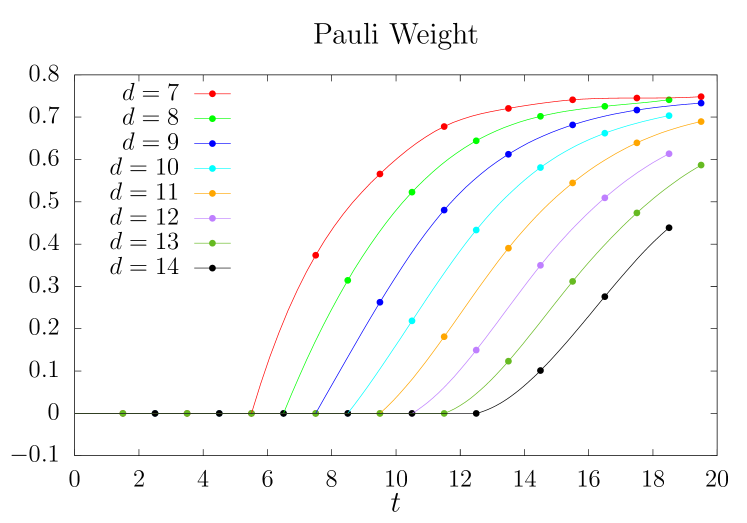
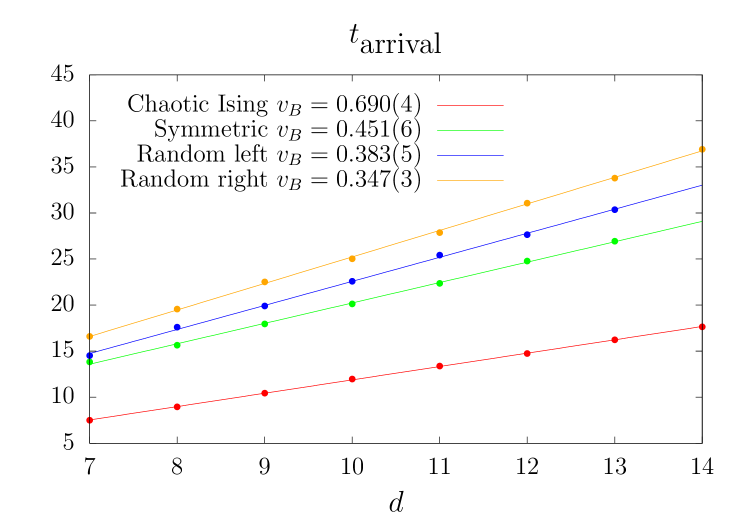
We use the Pauli weight roberts2015localized ; mezei2017entanglement ; jonay_coarse-grained_2018 to estimate in the Floquet circuit. The Pauli weight is defined to be the fraction of the operator weight at a site on non-identity operators. To minimize the number of distinct length scales affecting the data, we place at the leftmost site and probe its Pauli weight at the rightmost site :
| (166) | ||||
According to the operator spreading picture, the Pauli strings in the time-evolved operator spread to the right with mean velocity . Before the Pauli strings reach the right boundary, i.e. when , the Pauli weight is close to zero. At long times when , can be regarded as a random operator for the purpose of calculating the Pauli weight, which is then .
Fig. 18 shows the Pauli weight for the kicked Ising model with the parameters in Eq. 82. Due to the circuit structure, the Pauli weights at consecutive integer time steps are equal. Hence we place the data at half integer points, and interpolate the curve (with cubic spline) when the data is greater than zero. Following Ref. jonay_coarse-grained_2018 , we define as the time when the interpolated curve is at . Fitting with gives us an estimation of . Fig. 18 shows the results of fitting for the generic symmetric gate and the fixed but randomly chosen gate (Sec. V.1) and for the kicked Ising model (Eq. 82).
B.4 The approximate entanglement velocity
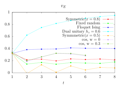
The second Rényi entropy after a quench corresponds to a free boundary condition at the bottom for the domain wall. Therefore the system will select out as the entanglement speed for . We extract the approximate entanglement speed from our numerical calculation of , and show its dependence on the truncation time in in Fig. 19.
All the curves start off for at the purity velocity of the random circuit. Differences between the gates then drive the curves to their respective entanglement velocities, either above or below the value at .
Notably, the curve for the dual-unitary gate shows a clear trend towards the analytical result . Curves for the Floquet Ising model, the generic reflection symmetric gate and the fixed random gate behave reasonably well. Fluctuations are still visible for up to , and it is hard to determine the functional form for convergence directly from this plot. However in the next subsection we will give evidence for exponential suppression of the irreducible step weights in these models at large .
We also include in the plot a continuous time model with a static Hamiltonian (the limit of the Floquet model with a sinusoidal field, Eq. 109). This model would require a separate theoretical analysis and we include it only for comparison. Due to continuous time translation symmetry it has a diffusive conserved energy density. This is expected to suppress to zero for the second Rényi entropy rakovszky2019sub ; huang2019dynamics ; zhou2019diffusive , and is likely to introduce parametrically larger (in ) finite time effects.121212We expect that for will still be nontrivial. The suppression of all the way to zero is due to rare Feynman trajectories in which a large spatial region is depleted of energy and cannot entangle. Since the dynamics of the energy density is diffusive, these empty regions can persist for a long time along a ray at , suppressing the cost of a membrane with , but not along a ray at nonzero .
B.5 The suppression of irreducible weights
In Sec. III.1, we conjectured that clusters inside a thick domain wall are exponentially suppressed at large , leading in turn to an exponential suppression of the irreducible step weights at large . We showed this explicitly for a typical fixed realization of a random circuit at large : there, long steps of size are suppressed by compared to the leading order contributions to the domain wall free energy on this scale.
Here we examine the nature of the decay in step weights at large numerically for translation-invariant spin-1/2 models. Quantitatively, we can compare with , where the former represents the irreducible step weight for a single step of size , while the latter represents the asymptotic scaling of the partition function for a domain wall of duration . Their ratio should decay exponentially according to our conjecture.
In Fig. 20, we plot along with both and as comparison. The best case is the dual unitary circuit, where a faster exponential decay of w.r.t. both and is clearly visible. The Floquet Ising model follows a similar trend. Though this is less clear for the reflection symmetric gate at , that is consistent with the fact that this gate is more weakly entangling than the others (Fig. 19) and takes larger to reach convergence.
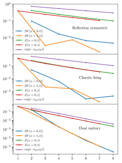
B.6 Diffusive character of the domain wall
In Sec. VI we argued that for generic choices of gate the wandering of the domain wall was diffusive at large scales. One consequence of this is the scaling in Eq. 85: . We stated in the caption to Fig. 12 that the data was in good agreement with this scaling. This is demonstrated in Fig. 21 which shows versus on a log-log plot.
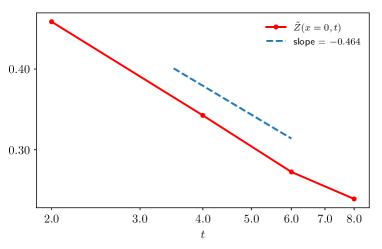
Appendix C Relation between root and line-tension
We give details of the relation between and the root described in Sec. IV.1. Let
| (167) |
This is the partition function with a fixed force on the endpoint rather than a fixed endpoint. Asymptotically, it should scale as
| (168) |
with jonay_coarse-grained_2018
| (169) |
so that and form a standard Legendre transform pair. On the other hand
| (170) |
Assuming that the smallest root of for a given is , then for
| (171) |
Matching the expansions in ,
| (172) |
Finally, inverting the Legendre transform yields the expression (63) in the main text for .
Appendix D The continuum equation for
For completeness, let us give a more general derivation of the continuum equation which makes contact with the equation in Ref. jonay_coarse-grained_2018, for the dynamical evolution of the state entanglement. Writing , we assume that the solution is such that higher derivatives of are small at late times (to be checked self-consistently), and expand in derivatives.
So far, we have considered a domain wall which is tethered at both the top and the bottom. To compute the entanglement of a state across an entanglement cut at position , we should instead take the domain wall to be tethered at position at the top, and free at the bottom; the initial condition is set by the entanglement in the initial state. The recursion relation still applies.
To save clutter, let us write instead of in the recursion relation. In terms of , it reads:
| (173) |
Expanding in the exponent gives
| (174) |
Generically, is of order , and are of order 1, and the higher derivatives are smaller. Therefore the leading order equation is simply
| (175) |
Using the definitions in Sec. IV.1, this is solved by
| (176) |
so that is the growth rate, which depends on the derivative of the entanglement as a function of the spatial location. We are interested in the subleading corrections to this equation. Let us define an -dependent “average” of an arbitrary function of the step:
| (177) |
From the relations for the generation functions,
| (178) |
We also define the associated velocity . By differentiating (178) with respect to , we have
| (179) |
This is the coarse grained velocity of the membrane since it also solves the Legendre transform (Eq. 63) relating the growth rate and the line tension .
We may then write (174) as
| (180) |
where the are higher derivatives. The exponent is now written in terms of quantities that are small at late times, so may be expanded,
| (181) |
We may use the leading-order solution to replace the time derivatives on the right hand side with space derivatives (cf. Eqs. 176, 179): and . Then
| (182) |
By differentiating (178) twice,
| (183) |
so
| (184) |
(The primes on indicate derivatives with respect to its argument.)
Appendix E Triangle weights for two commuting domain walls
For reference and use in App. A.5, here we list exact expressions for triangle weights . This corresponds to two incoming “commutating” elementary domain walls at the top of the triangle. (An elementary domain wall is a transposition.) We also list their order relative to the weight of two separated domain walls. We use the notation from Ref. zhou2019emergent, , drawing one line for each elementary domain wall crossing an edge of the triangle.
There are in total 6 classes. Within each class the configurations are related by the combination of reflection symmetry about the center axis, conjugation by , or both.
We categorize them in terms of :
-
1.
, .
(188) -
2.
,
(189) -
3.
,
(190) -
4.
, , , , , , ,
(191) -
5.
, , , , , , ,
(192) -
6.
,
(193)
References
- [1] Leo P Kadanoff and Paul C Martin. Hydrodynamic equations and correlation functions. Annals of Physics, 24:419–469, October 1963.
- [2] Pierre C Hohenberg and Bertrand I Halperin. Theory of dynamic critical phenomena. Reviews of Modern Physics, 49(3):435, 1977.
- [3] R Oliveira, OCO Dahlsten, and MB Plenio. Generic entanglement can be generated efficiently. Physical review letters, 98(13):130502, 2007.
- [4] Alioscia Hamma, Siddhartha Santra, and Paolo Zanardi. Quantum entanglement in random physical states. Physical review letters, 109(4):040502, 2012.
- [5] Fernando GSL Brandão, Aram W Harrow, and Michał Horodecki. Local random quantum circuits are approximate polynomial-designs. Communications in Mathematical Physics, 346(2):397–434, 2016.
- [6] Adam Nahum, Jonathan Ruhman, Sagar Vijay, and Jeongwan Haah. Quantum Entanglement Growth under Random Unitary Dynamics. Physical Review X, 7(3):031016, July 2017.
- [7] Adam Nahum, Sagar Vijay, and Jeongwan Haah. Operator spreading in random unitary circuits. Physical Review X, 8(2):021014, 2018.
- [8] C. W. von Keyserlingk, Tibor Rakovszky, Frank Pollmann, and S. L. Sondhi. Operator Hydrodynamics, OTOCs, and Entanglement Growth in Systems without Conservation Laws. Physical Review X, 8(2):021013, April 2018.
- [9] Tibor Rakovszky, Frank Pollmann, and C. W. von Keyserlingk. Diffusive Hydrodynamics of Out-of-Time-Ordered Correlators with Charge Conservation. Physical Review X, 8(3):031058, September 2018.
- [10] Vedika Khemani, Ashvin Vishwanath, and David A. Huse. Operator Spreading and the Emergence of Dissipative Hydrodynamics under Unitary Evolution with Conservation Laws. Physical Review X, 8(3):031057, September 2018.
- [11] Amos Chan, Andrea De Luca, and J. T. Chalker. Solution of a Minimal Model for Many-Body Quantum Chaos. Physical Review X, 8(4):041019, November 2018.
- [12] Amos Chan, Andrea De Luca, and J. T. Chalker. Spectral statistics in spatially extended chaotic quantum many-body systems. arXiv:1803.03841 [cond-mat, physics:hep-th, physics:quant-ph], March 2018.
- [13] Daniel A Rowlands and Austen Lamacraft. Noisy coupled qubits: Operator spreading and the fredrickson-andersen model. Physical Review B, 98(19):195125, 2018.
- [14] Tianci Zhou and Adam Nahum. Emergent statistical mechanics of entanglement in random unitary circuits. Physical Review B, 99(17):174205, 2019.
- [15] Tibor Rakovszky, Frank Pollmann, and C. W. von Keyserlingk. Sub-ballistic Growth of R\’enyi Entropies due to Diffusion. Physical Review Letters, 122(25):250602, June 2019.
- [16] Aaron J. Friedman, Amos Chan, Andrea De Luca, and J. T. Chalker. Spectral statistics and many-body quantum chaos with conserved charge. Physical Review Letters, 123(21):210603, November 2019.
- [17] Nicholas Hunter-Jones. Unitary designs from statistical mechanics in random quantum circuits. arXiv:1905.12053 [cond-mat, physics:hep-th, physics:quant-ph], May 2019.
- [18] Cheryne Jonay, David A. Huse, and Adam Nahum. Coarse-grained dynamics of operator and state entanglement. arXiv:1803.00089 [cond-mat, physics:hep-th, physics:nlin, physics:quant-ph], February 2018. arXiv: 1803.00089.
- [19] Elliott H Lieb and Derek W Robinson. The finite group velocity of quantum spin systems. In Statistical Mechanics, pages 425–431. Springer, 1972.
- [20] Pasquale Calabrese and John Cardy. Evolution of entanglement entropy in one-dimensional systems. Journal of Statistical Mechanics: Theory and Experiment, 2005(04):P04010, 2005.
- [21] Hyungwon Kim and David A Huse. Ballistic spreading of entanglement in a diffusive nonintegrable system. Physical review letters, 111(12):127205, 2013.
- [22] A. Kitaev. Hidden correlations in the hawking radiation and thermal noise. In Talk given at the Fundamental Physics Prize Symposium, 2014.
- [23] Hong Liu and S Josephine Suh. Entanglement tsunami: universal scaling in holographic thermalization. Physical review letters, 112(1):011601, 2014.
- [24] Stephen H. Shenker and Douglas Stanford. Black holes and the butterfly effect. Journal of High Energy Physics, 2014(3):67, March 2014.
- [25] Daniel A Roberts, Douglas Stanford, and Leonard Susskind. Localized shocks. Journal of High Energy Physics, 2015(3):51, 2015.
- [26] Juan Maldacena, Stephen H. Shenker, and Douglas Stanford. A bound on chaos. Journal of High Energy Physics, 2016(8):106, August 2016.
- [27] Daniel A. Roberts and Brian Swingle. Lieb-Robinson Bound and the Butterfly Effect in Quantum Field Theories. Physical Review Letters, 117(9):091602, August 2016.
- [28] Adam M Kaufman, M Eric Tai, Alexander Lukin, Matthew Rispoli, Robert Schittko, Philipp M Preiss, and Markus Greiner. Quantum thermalization through entanglement in an isolated many-body system. Science, 353(6301):794–800, 2016.
- [29] Igor L Aleiner, Lara Faoro, and Lev B Ioffe. Microscopic model of quantum butterfly effect: out-of-time-order correlators and traveling combustion waves. Annals of Physics, 375:378–406, 2016.
- [30] Aavishkar A Patel and Subir Sachdev. Quantum chaos on a critical fermi surface. Proceedings of the National Academy of Sciences, 114(8):1844–1849, 2017.
- [31] Pavan Hosur, Xiao-Liang Qi, Daniel A. Roberts, and Beni Yoshida. Chaos in quantum channels. Journal of High Energy Physics, 2016(2):1–49, February 2016.
- [32] Márk Mezei. On entanglement spreading from holography. Journal of High Energy Physics, 2017(5):64, 2017.
- [33] Pavel Kos, Marko Ljubotina, and Tomaž Prosen. Many-Body Quantum Chaos: Analytic Connection to Random Matrix Theory. Physical Review X, 8(2):021062, June 2018.
- [34] Márk Mezei and Julio Virrueta. Exploring the Membrane Theory of Entanglement Dynamics. December 2019.
- [35] Bruno Bertini, Pavel Kos, and Tomaž Prosen. Entanglement Spreading in a Minimal Model of Maximal Many-Body Quantum Chaos. Physical Review X, 9(2):021033, May 2019.
- [36] Lorenzo Piroli, Bruno Bertini, J. Ignacio Cirac, and Tomaz Prosen. Exact dynamics in dual-unitary quantum circuits. arXiv:1911.11175 [cond-mat, physics:quant-ph], November 2019.
- [37] Márk Mezei. Membrane theory of entanglement dynamics from holography. Physical Review D, 98(10):106025, November 2018.
- [38] Shinsei Ryu and Tadashi Takayanagi. Holographic derivation of entanglement entropy from the anti–de sitter space/conformal field theory correspondence. Physical review letters, 96(18):181602, 2006.
- [39] Veronika E Hubeny, Mukund Rangamani, and Tadashi Takayanagi. A covariant holographic entanglement entropy proposal. Journal of High Energy Physics, 2007(07):062, 2007.
- [40] Cesar A Agón and Márk Mezei. Bit threads and the membrane theory of entanglement dynamics. arXiv preprint arXiv:1910.12909, 2019.
- [41] Michael Freedman and Matthew Headrick. Bit threads and holographic entanglement. Communications in Mathematical Physics, 352(1):407–438, May 2017.
- [42] Patrick Hayden, Sepehr Nezami, Xiao-Liang Qi, Nathaniel Thomas, Michael Walter, and Zhao Yang. Holographic duality from random tensor networks. Journal of High Energy Physics, 2016(11):9, 2016.
- [43] Romain Vasseur, Andrew C. Potter, Yi-Zhuang You, and Andreas W. W. Ludwig. Entanglement transitions from holographic random tensor networks. Physical Review B, 100(13):134203, October 2019.
- [44] Hyungwon Kim, Tatsuhiko N. Ikeda, and David A. Huse. Testing whether all eigenstates obey the eigenstate thermalization hypothesis. Physical Review E, 90(5):052105, November 2014.
- [45] Tomaž Prosen. Chaos and complexity of quantum motion. Journal of Physics A: Mathematical and Theoretical, 40(28):7881, 2007.
- [46] Sarang Gopalakrishnan and Austen Lamacraft. Unitary circuits of finite depth and infinite width from quantum channels. Physical Review B, 100(6):064309, August 2019.
- [47] Bruno Bertini, Pavel Kos, and Tomaž Prosen. Exact Correlation Functions for Dual-Unitary Lattice Models in $1+1$ Dimensions. Physical Review Letters, 123(21):210601, November 2019.
- [48] M. Akila, D. Waltner, B. Gutkin, and T. Guhr. Particle-time duality in the kicked Ising spin chain. Journal of Physics A: Mathematical and Theoretical, 49(37):375101, August 2016.
- [49] Bruno Bertini, Pavel Kos, and Tomaž Prosen. Operator entanglement in local quantum circuits i: Maximally chaotic dual-unitary circuits. arXiv preprint arXiv:1909.07407, 2019.
- [50] Benoît Collins and Piotr Śniady. Integration with Respect to the Haar Measure on Unitary, Orthogonal and Symplectic Group. Communications in Mathematical Physics, 264(3):773–795, March 2006. bibtex: collins_integration_2006.
- [51] Yinzheng Gu. Moments of Random Matrices and Weingarten Functions. Thesis, Queen’s University, September 2013.
- [52] Don Weingarten. Asymptotic behavior of group integrals in the limit of infinite rank. Journal of Mathematical Physics, 19(5):999–1001, 1978.
- [53] Aram W. Harrow. The Church of the Symmetric Subspace. arXiv:1308.6595 [quant-ph], August 2013. arXiv: 1308.6595.
- [54] Paolo Zanardi. Entanglement of quantum evolutions. Phys. Rev. A, 63:040304, Mar 2001.
- [55] Tomaž Prosen and Iztok Pižorn. Operator space entanglement entropy in a transverse Ising chain. Physical Review A, 76(3):032316, September 2007.
- [56] Iztok Pižorn and Tomaž Prosen. Operator space entanglement entropy in $XY$ spin chains. Physical Review B, 79(18):184416, May 2009.
- [57] J. Dubail. Entanglement scaling of operators: a conformal field theory approach, with a glimpse of simulability of long-time dynamics in 1+1d. Journal of Physics A: Mathematical and Theoretical, 50(23):234001, May 2017.
- [58] Tianci Zhou and David J. Luitz. Operator entanglement entropy of the time evolution operator in chaotic systems. Physical Review B, 95(9), March 2017. arXiv: 1612.07327.
- [59] Paolo Zanardi, Christof Zalka, and Lara Faoro. Entangling power of quantum evolutions. Physical Review A, 62(3):030301, August 2000.
- [60] John Cardy. Renormalisation group theory of branching potts interfaces. Nuclear Physics B, 565(3):506–520, 2000.
- [61] David A. Huse, Christopher L. Henley, and Daniel S. Fisher. Huse, henley, and fisher respond. Phys. Rev. Lett., 55:2924–2924, Dec 1985.
- [62] Mehran Kardar, Giorgio Parisi, and Yi-Cheng Zhang. Dynamic Scaling of Growing Interfaces. Physical Review Letters, 56(9):889–892, March 1986.
- [63] Charles Stahl, Vedika Khemani, and David A Huse. Asymmetric butterfly velocities in hamiltonian and circuit models. arXiv preprint arXiv:1812.05589, 2018.
- [64] Yong-Liang Zhang and Vedika Khemani. Asymmetric butterfly velocities in 2-local hamiltonians. arXiv preprint arXiv:1909.03988, 2019.
- [65] B Kraus and JI Cirac. Optimal creation of entanglement using a two-qubit gate. Physical Review A, 63(6):062309, 2001.
- [66] Navin Khaneja and Steffen Glaser. Cartan Decomposition of SU(2n̂), Constructive Controllability of Spin systems and Universal Quantum Computing. arXiv:quant-ph/0010100, October 2000.
- [67] Bruno Bertini, Pavel Kos, and Tomaž Prosen. Exact Spectral Form Factor in a Minimal Model of Many-Body Quantum Chaos. Physical Review Letters, 121(26):264101, December 2018.
- [68] Vedika Khemani, David A. Huse, and Adam Nahum. Velocity-dependent Lyapunov exponents in many-body quantum, semi-classical, and classical chaos. arXiv:1803.05902 [cond-mat, physics:hep-th, physics:nlin, physics:quant-ph], March 2018. arXiv: 1803.05902.
- [69] Adam Nahum, Sthitadhi Roy, Sagar Vijay, and Tianci Zhou. Chaos and the time-ordered two-point function, forthcoming.
- [70] Ewan McCulloch and C. W. von Keyserlingk. Forthcoming.
- [71] Elliott H. Lieb and Derek W. Robinson. The finite group velocity of quantum spin systems. Communications in Mathematical Physics, 28(3):251–257, September 1972.
- [72] Yichen Huang. Dynamics of Renyi entanglement entropy in local quantum circuits with charge conservation. arXiv:1902.00977 [cond-mat, physics:hep-th, physics:quant-ph], February 2019.
- [73] Tianci Zhou and Andreas WW Ludwig. On the diffusive scaling of r’enyi entanglement entropy. arXiv preprint arXiv:1911.12384, 2019.
- [74] Marko Znidaric. Entanglement growth in diffusive systems. arXiv:1912.03645 [cond-mat], December 2019.
- [75] Hong Liu and Paolo Glorioso. Lectures on non-equilibrium effective field theories and fluctuating hydrodynamics. page 008, July 2018.
- [76] Mukund Rangamani. Gravity & Hydrodynamics: Lectures on the fluid-gravity correspondence. arXiv:0905.4352 [gr-qc, physics:hep-th, physics:physics], October 2009. arXiv: 0905.4352.
- [77] Amos Chan, Andrea De Luca, and J. T. Chalker. Spectral Statistics in Spatially Extended Chaotic Quantum Many-Body Systems. Physical Review Letters, 121(6):060601, August 2018.
- [78] Yaodong Li, Xiao Chen, and Matthew Fisher. Measurement-driven entanglement transition in hybrid quantum circuits. arXiv preprint arXiv:1901.08092, 2019.
- [79] Michael J Gullans and David A Huse. Dynamical purification phase transition induced by quantum measurements. arXiv preprint arXiv:1905.05195, 2019.
- [80] Aram W Harrow and Richard A Low. Random quantum circuits are approximate 2-designs. Communications in Mathematical Physics, 291(1):257–302, 2009.
- [81] Daniel A Roberts and Beni Yoshida. Chaos and complexity by design. Journal of High Energy Physics, 2017(4):121, 2017.
- [82] Jordan Cotler, Nicholas Hunter-Jones, Junyu Liu, and Beni Yoshida. Chaos, complexity, and random matrices. Journal of High Energy Physics, 2017(11):48, 2017.
- [83] Brian Skinner, Jonathan Ruhman, and Adam Nahum. Measurement-induced phase transitions in the dynamics of entanglement. Phys. Rev. X, 9:031009, Jul 2019.
- [84] Yaodong Li, Xiao Chen, and Matthew PA Fisher. Quantum zeno effect and the many-body entanglement transition. Physical Review B, 98(20):205136, 2018.
- [85] Amos Chan, Rahul M. Nandkishore, Michael Pretko, and Graeme Smith. Unitary-projective entanglement dynamics. Phys. Rev. B, 99:224307, Jun 2019.
- [86] Soonwon Choi, Yimu Bao, Xiao-Liang Qi, and Ehud Altman. Quantum error correction and entanglement phase transition in random unitary circuits with projective measurements. arXiv preprint arXiv:1903.05124, 2019.
- [87] M. Szyniszewski, A. Romito, and H. Schomerus. Entanglement transition from variable-strength weak measurements. Phys. Rev. B, 100:064204, Aug 2019.
- [88] Xiangyu Cao, Antoine Tilloy, and Andrea De Luca. Entanglement in a fermion chain under continuous monitoring. SciPost Phys., 7:24, 2019.
- [89] Michael J Gullans and David A Huse. Scalable probes of measurement-induced criticality. arXiv preprint arXiv:1910.00020, 2019.
- [90] Qicheng Tang and W Zhu. Measurement-induced phase transition: A case study in the non-integrable model by density-matrix renormalization group calculations. arXiv preprint arXiv:1908.11253, 2019.
- [91] Yimu Bao, Soonwon Choi, and Ehud Altman. Theory of the phase transition in random unitary circuits with measurements. arXiv preprint arXiv:1908.04305, 2019.
- [92] Chao-Ming Jian, Yi-Zhuang You, Romain Vasseur, and Andreas WW Ludwig. Measurement-induced criticality in random quantum circuits. arXiv preprint arXiv:1908.08051, 2019.
- [93] Aidan Zabalo, Michael J Gullans, Justin H Wilson, Sarang Gopalakrishnan, David A Huse, and JH Pixley. Critical properties of the measurement-induced transition in random quantum circuits. arXiv preprint arXiv:1911.00008, 2019.
- [94] Márk Mezei and Douglas Stanford. On entanglement spreading in chaotic systems. Journal of High Energy Physics, 2017(5):65, 2017.
- [95] Tibor Rakovszky, Frank Pollmann, and CW Von Keyserlingk. Sub-ballistic growth of rényi entropies due to diffusion. Physical review letters, 122(25):250602, 2019.
- [96] Yichen Huang. Dynamics of renyi entanglement entropy in local quantum circuits with charge conservation. arXiv preprint arXiv:1902.00977, 2019.