Composite-fringe atom interferometry for high dynamic-range sensing

Abstract

Atom interferometers offer excellent sensitivity to gravitational and inertial signals but have limited dynamic range. We introduce a scheme that improves this trade-off by a factor of 50 using composite, moiré-like, fringes, obtained from sets of measurements with slightly varying interrogation times. We analyze analytically the performance gain in this approach and the trade-offs it entails between sensitivity, dynamic range, and bandwidth, and we experimentally validate the analysis over a wide range of parameters. Combining composite-fringe measurements with a particle-filter estimation protocol, we demonstrate continuous tracking of a rapidly varying signal over a span two orders of magnitude larger than the dynamic range of a traditional atom interferometer.

I Introduction

Atom interferometry (AI) (Tino and Kasevich, 2014) enables highly sensitive and accurate sensing of gravitational (Peters et al., 2001; Snadden et al., 1998; Sorrentino et al., 2012) and inertial forces (Barrett et al., 2014; Canuel et al., 2006; Stockton et al., 2011; Gustavson et al., 1997; Dickerson et al., 2013; Savoie et al., 2018). In addition to laboratory-based experiments in fundamental physics, such as tests of general relativity (Dimopoulos et al., 2007; Müller et al., 2010; Hohensee et al., 2011; Aguilera et al., 2014; Zhou et al., 2015) and precision measurement of physical constants (Weiss et al., 1993; Fixler et al., 2007; Bouchendira et al., 2011; Rosi et al., 2014; Parker et al., 2018), AIs for field-applications are being developed worldwide (Bongs et al., 2019). Mobile atomic gravimeters and gravity-gradiometers (Wu, 2009; Bidel et al., 2013; Farah et al., 2014; Freier et al., 2016; Barrett et al., 2016; Ménoret et al., 2018; Zhu, 2018; Becker et al., 2018; Wu et al., 2019; Lamb, 2019) have been demonstrated for geophysical surveys on land (Wu, 2009; Wu et al., 2019), at sea (Bidel et al., 2018), and in the air (Bidel et al., ), while cold atom accelerometers and gyroscopes are developed for inertial navigation (Rakholia et al., 2014; Cheiney et al., 2018; Chen et al., 2019). Such applications motivate the development of advanced AI techniques for robust operation under conditions of large uncertainty and large temporal variations in the measured signal.

As a phase-measuring instrument, a trade-off exists between an AI sensitivity and its ambiguity-free dynamic range. The ratio of dynamic range to sensitivity is in general fixed by the signal-to-noise ratio (SNR), whereas the scale factor, which determines their absolute values, may be controlled by changing the interferometer interrogation time $T$. When prior knowledge of the measured signal is insufficient, a standard approach involves initial measurements with low sensitivity and high dynamic range (short $T$) and gradual progress to measurements with high sensitivity and low dynamic range (long $T$) (Wu et al., 2019). However, the time-averaged sensitivity per $\sqrt{\text{Hz}}$ of this sequence is greatly reduced. Alternatively, simultaneous measurements using two interrogation times was demonstrated in a dual-species interferometer (Bonnin et al., 2018) with an improved dynamic range of $\times 5$ at the cost of added experimental complexity. Ambiguities of AIs may also be resolved by hybridization with classical sensors with large dynamic range (Merlet et al., 2009; Lautier et al., 2014), especially relevant when the measured signal varies continuously in time and substantially changes from shot to shot. However, imperfections such as non-linearity of the classical sensors, transfer function errors and misalignment may limit the usefulness of this technique in harsh conditions (Bidel et al., 2018), necessitating prolonged operation at short $T$ at the expense of sensitivity.

In this work, we introduce an approach to AI which increases its dynamic range with minor penalty on sensitivity. We perform a set of measurements with slightly varying values of $T$, corresponding to slightly different interferometer scale factors. Together, as in a moiré effect, these measurements constitute a composite fringe whose frequency, as well as its phase, encodes the measured inertial signal, providing a non-ambiguous dynamic range larger than measurements with a fixed $T$. The increase in dynamic range scales inversely with the span of scale factors and can reach orders of magnitude, limited only by the experimental SNR. In addition to a static demonstration, we apply the scheme together with a particle-filter estimator to successfully track rapidly-varying signals, which change by more than $2\pi$ between consecutive measurements and span hundreds of radians altogether, while maintaining high sensitivity.

II Experimental setup

We apply the composite fringe approach in a Mach-Zehnder AI which measures gravitational acceleration (Kasevich and Chu, 1991). A freely-falling cold-atom ensemble interacts with pulses of counter-propagating laser beams which stimulate two-photon transitions. A sequence of three pulses spatially splits, redirects, and recombines the atomic wavepackets [Fig. 1(a)]. The interferometer phase is $\phi=\left(k_{\textrm{eff}}g-\alpha\right)T^{2}+\phi_{L}$, where $k_{\textrm{eff}}$ is the effective atom optics two-photon wavevector, $g$ is the gravitational acceleration, and $T$ is the time between pulses. The relative frequency of the counter-propagating beams is chirped at a rate $\alpha=k_{\textrm{eff}}g_{0}$, where $g_{0}$ is an approximate value of $g$, to compensate the changing Doppler shift of the falling atoms. $\phi_{L}$ is a tunable laser phase applied during the final $\pi/2$-pulse.

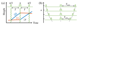
Figure 1: (a) Schematic diagram of an atomic gravimeter, operating in a $\pi/2$-$\pi$-$\pi/2$ Mach-Zehnder geometry. Counter-propagating laser beams interact with the atoms and generate the interferometer sequence. (b) Composite-fringe AI comprises a set a of measurements with interrogation times $T$ that vary quadratically within a small range.

Our apparatus is described in detail in Ref. [Yankelev et al., 2019]. Briefly, we trap and cool ${}^{87}\textrm{Rb}$ atoms and launch them upwards using moving optical molasses. Vertical, retroreflected Raman beams, derived from a single laser modulated at $6.834\,\textrm{GHz}$, drive Doppler-sensitive two-photon transitions (Kasevich et al., 1991) between $\left|F=1,m_{F}=0\right\rangle$ and $\left|F=2,m_{F}=0\right\rangle$ for state initialization and interferometry sequence. The population fraction in $F=2$, determined by state-dependent fluorescence, constitutes the interferometer output signal.

III Composite fringe analysis and performance

The standard fringe of an AI is $S\left(\phi\right)=A-\left(C/2\right)\cos\phi$, where $A$ and $C$ are the fringe offset and contrast. By measuring this fringe at $N$ points (scanning either $\alpha$ or $\phi_{L}$) at a fixed $T$, the gravitational phase $k_{\textrm{eff}}gT^{2}$ is determined with uncertainty $\sigma_{\phi}/\sqrt{N}$, with $\sigma_{\phi}$ the total phase uncertainty per shot (see Appendix A). Therefore, gravity is determined with uncertainty per shot $\sigma_{g,\textrm{standard}}=\sigma_{\phi}/\left(k_{\textrm{eff}}T^{2}\right)$, over an ambiguity-free dynamic range $\Delta g_{\textrm{standard}}=2\pi/\left(k_{\textrm{eff}}T^{2}\right)$. The ratio of dynamic range to sensitivity-per-shot is $\left(\Delta g/\sigma_{g}\right)_{\textrm{standard}}=2\pi/\sigma_{\phi}$, depending only on the measurement phase uncertainty.

Here instead, we form a composite fringe from a set of $N$ measurements $S_{n}$, varying the scale factor $k_{\textrm{eff}}T^{2}$ linearly by choosing variable interrogation times [Fig. 1(b)],

$$T_{n}^{2}=T_{\textrm{min}}^{2}+n\frac{T_{\textrm{max}}^{2}-T_{\textrm{min}}^{2}}{N-1}\,\,\,\,\,\textrm{for}\,\,\,\,n=0,\ldots,N-1,$$ (1)

with $T_{\textrm{min}}<T_{\textrm{max}}$, keeping $\alpha$ and $\phi_{L}$ fixed. As Figs. 2(a),(b) show, the series $\left\{S_{n}\right\}$ forms a composite fringe, $S_{n}=A-\left(C/2\right)\cos\left(n\omega_{\textrm{comp}}+\phi_{\textrm{comp}}\right)$, with

$$\phi_{\textrm{comp}} =\left(k_{\textrm{eff}}g-\alpha\right)T_{\textrm{min}}^{2}+\phi_{L},$$ (2)

$$\omega_{\textrm{comp}} =\left(k_{\textrm{eff}}g-\alpha\right)\frac{T_{\textrm{max}}^{2}-T_{\textrm{min}}^{2}}{N-1}.$$ (3)

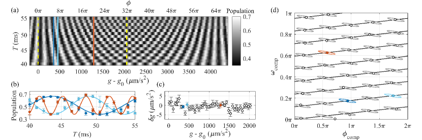
Figure 2: Composite-fringe AI. (a) Experimental data using $N=16$ interrogation times between $T_{\min}=40\,\mathrm{ms}$ and $T_{\max}=55\,\mathrm{ms}$. Different gravity values are simulated by changing the Raman beams chirp rate $\alpha=k_{\textrm{eff}}g_{0}$. The ambiguity-free dynamic range (dashed lines) is extended by the composite-fringe approach to $32\pi\,\mathrm{rad}$ at $T_{\max}$, representing a 16-fold increase compared to standard measurements. Data is averaged over 5 shots. (b) Composite fringes measured at different gravity values as indicated by colored lines in (a). Proximate gravity values (dark, bright blue) result in fringes with similar frequency but different phase, while a larger difference in gravity (red) renders a substantial change in frequency. Dots are measurements averaged over 5 shots, error bars are $\pm 1\sigma$, solid lines are sinusoidal fits. (c) Residual of the gravity value fitted from each composite fringe, over the span of one extended dynamic range. Resulting sensitivity is $1.7\,\mathrm{\mu m/s^{2}}$ per fringe, or $6.7\,\mathrm{\mu m/s^{2}}$ per shot, comparable to $7.3\,\mathrm{\mu m/s^{2}}$ per shot using standard fringes at fixed $T=T_{\max}$ in our apparatus. Residuals have mean $-0.3\pm 0.4\left(2\sigma\right)\,\mathrm{\mu m/s^{2}}$, consistent with no added bias. (d) Phase-frequency map of composite fringes: circles represent the phase and frequency extracted from fits to the fringe data in (a), solid lines are the predicted loci of measurements within the extended dynamic range. Gravity increases from bottom left to top right. Ellipses represent the covariance matrix of phase and frequency estimation with the experimentally-characterized $\sigma_{\phi}=400\,\mathrm{mrad}$ at 95% confidence interval.

Unlike standard fringes with fixed $T$, here both phase and frequency depend on $g$, albeit with very different scaling: $\phi_{\textrm{comp}}$ varies rapidly with $g$ and represents a high-resolution measurement, similar to standard measurements with fixed $T$, whereas $\omega_{\textrm{comp}}$ varies slowly with $g$ and represents a coarse measurement [Fig. 2(d)]. This beat frequency, which is revealed by varying $T$, provides the extended dynamic range and stands in close analogy to moiré interferometry (Oberthaler et al., 1996; Cronin et al., 2009), while the phase of the composite fringe is still accessible and provides the high sensitivity.

The composite-fringe frequency can be estimated unambiguously up to $\omega_{\textrm{comp}}=\pi$, resulting in the extended dynamic range $\Delta g_{\textrm{comp}}=\pi\left(N-1\right)/\left[k_{\textrm{eff}}\left(T_{\textrm{max}}^{2}-T_{\textrm{min}}^{2}\right)\right]$. With respect to a fixed-$T$ measurement, the dynamic range increases by a factor

$$\frac{\Delta g_{\textrm{comp}}}{\Delta g_{\textrm{standard}}} =\frac{1}{2}\frac{N-1}{1-T_{\textrm{min}}^{2}/T_{\textrm{max}}^{2}}.$$ (4)

At the same time, the gravity sensitivity per shot of a composite fringe is approximately (see Appendix A)

$$\sigma_{g,\textrm{comp}}\approx\frac{\sigma_{\phi}}{k_{\textrm{eff}}T_{\min}T_{\max}}=\frac{T_{\max}}{T_{\min}}\cdot\sigma_{g,\textrm{standard}}.$$ (5)

For $T_{\min}$ approaching $T_{\max}$, the dynamic range enhancement is significant while the penalty in $\sigma_{g,\textrm{comp}}$ is small. Indeed, Fig. 2(c) presents the gravity residuals $\delta g$ obtained from fits of the measured composite fringes, exhibiting similar sensitivity to measurements at fixed $T=T_{\max}$ with no observed systematic bias.

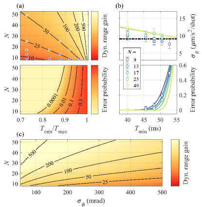
Figure 3: (a) Projected performance of composite fringes compared to standard measurement at fixed $T$. Top: Dynamic range enhancement [Eq. 4]. Bottom: Error probability [Eq. A11 in Appendix A, evaluated with $\sigma_{\phi}=400\,\mathrm{mrad}$]. (b) Experimental results: Sensitivity per shot (top) and error probability (bottom) as a function of $T_{\min}$, with $T_{\max}=55\,\mathrm{ms}$, for different $N$ as indicated in the legend. Measurements (circles) are averaged over 230 composite fringes, error bars represent 68% confidence interval. The results are in excellent agreement with the analytic predictions (solid lines). Dashed line represents a reference measurement with fixed $T=55\,\mathrm{ms}$. Increase in dynamic range at the measured settings is indicated by filled circles in (a). (c) Projected gain in dynamic range as a function of $\sigma_{\phi}$ and $N$, for $10^{-2}$ error probability threshold.

The potential gain in dynamic range is limited by $\sigma_{\phi}$. Primarily, when the uncertainty in estimating the composite fringe phase and frequency is comparable to the line separation in Fig. 2(d), a line jump may occur, resulting in a large error in estimating $g$. The criterion for avoiding large errors is approximately (see Appendix A)

$$\frac{\sqrt{N}}{\sigma_{\phi}}\frac{\left(T_{\textrm{max}}^{2}-T_{\textrm{min}}^{2}\right)}{T_{\textrm{min}}T_{\textrm{max}}}\gg 1.$$ (6)

Notably, the potential gain in dynamic range increases if $\sigma_{\phi}$ decreases, as $T_{\textrm{min}}$ can approach $T_{\textrm{max}}$ without increasing the error probability. Conversely, the error probability may be reduced by increasing $N$, which also serves to increase the dynamic range, at the cost of temporal bandwidth. We note that in the limit of $T_{\textrm{min}}=T_{\textrm{max}}$, Eq. (6) cannot be satisfied for finite $\sigma_{\phi}$, however such measurements can still be analyzed as in traditional AI within the original dynamic range $\Delta g_{\textrm{standard}}$, recovering the standard measurement scheme at fixed $T$.

To understand the trade-offs in the composite fringe approach, we present in Fig. 3(a) the projected dynamic range enhancement compared to fixed-$T$ measurements and the corresponding error probability. The latter was evaluated for total phase uncertainty $\sigma_{\phi}=400\,\mathrm{mrad}$, which was experimentally characterized in our apparatus for $T\sim 50\,\mathrm{ms}$ and is primarily due to vibrations. Operating at $N\lesssim 20$, corresponding to typical AI temporal bandwidths, and requiring error probabilities below $10^{-2}$, we can operate at $T_{\min}/T_{\max}\approx 0.85$ and gain more than an order of magnitude in dynamic range. For larger $N$, ratios $T_{\min}/T_{\max}$ of over $0.9$ become possible, enabling gains of over two orders of magnitude.

To verify the model, we measured hundreds of composite fringes between $T_{\min}=40\,\mathrm{ms}$ and $T_{\max}=55\,\mathrm{ms}$ over $N=49$ points at a constant chirp rate, and analyzed the results in subsets of different $N$ and $T_{\min}$ values. Measurements at fixed $T=55\,\mathrm{ms}$ were also performed for reference. Figure 3(b) shows that the data are in excellent agreement with the analytical model with no fit parameters.

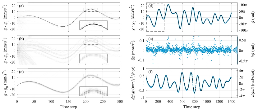
Figure 4: Experimental results of composite fringe and particle filtering with a dynamic signal. (a) Time-dependent, weighted particle distribution for composite-fringe AI ($N=12,\thinspace T_{\min}=20\,\mathrm{ms},\thinspace T_{\max}=30\,\mathrm{ms}$, corresponding to $\Delta g_{\textrm{comp}}=4.3\,\mathrm{mm/s^{2}}$). Columns represent the weighted histogram of $g_{m,i}$ at each time step. Particles are initialized at $g_{m,0}=g_{0}$, $\dot{g}_{m,0}=0$ with uncertainties $\sigma_{g,0}=5\,\mathrm{mm/s^{2}}$, $\sigma_{\dot{g},0}=1.5\,\mathrm{mm/s^{2}/\textrm{shot}}$. (b) Particle filter analysis of standard fixed-$T$ measurements ($T=30\,\mathrm{ms}$), same initial conditions as in (a). (c) Same as (b), with ideal initial conditions and zero initial uncertainty. Insets depict the single solution found by the filter using the composite-fringe approach versus the ambiguity of standard fixed-$T$ measurements. (d) Estimated gravity signal from our offline analysis protocol (blue; see Appendix B) compared to the known input signal (black). Changes in $g$ correspond to $\pm 100\pi\,\mathrm{rad}$ at $T_{\max}$, a hundred-fold improvement in dynamic range. Dashed lines indicate the region shown in (a). (e) Estimated signal residuals, with $\sigma_{g}=17\,\mathrm{\mu m/s^{2}}$ per shot, consistent with the expected $15\,\mathrm{\mu m/s^{2}}$ per shot at these experimental conditions. (f) $\dot{g}$ estimated by the filter (blue) compared to the input signal (black). Shot-to-shot changes of up to $\pm 3\pi\,\mathrm{rad/shot}$ at $T_{\max}$ are evident.

Figure 3(c) summarizes the dynamic range enhancement for different values of phase uncertainty, at a fixed error probability threshold of $10^{-2}$, a value where large errors may be removed with outlier detection with little sacrifice in sensitivity or bandwidth. A large, realistic parameter space exists where the dynamic range increases by more than $\times 100$ at high temporal bandwidth.

IV Time-varying signals

The analysis thus far assumes a static or slowly varying signal with respect to the measurement time of an $N$-point composite fringe, as in stationary gravity measurements. We now turn our focus to dynamic scenarios, such as mobile gravity surveys or inertial measurements on navigating platforms, where the measured signal may change by more than $\pm\pi$ from shot to shot and result in phase ambiguities. To address this challenge and track a dynamic signal, we combine the composite-fringe approach with an estimation protocol employing particle-filter methodology.

Particle filtering is a Bayesian estimation protocol based on a sequential Monte-Carlo method (Moral, 1996; Merwe et al., 2001), where a large set of weighted particles is used to estimate the posterior distribution of unknown state-variables based on inaccurate observations or measurements. This approach is especially suited for problems with multimodal likelihood functions, such as ambiguous phase measurements, where the resulting (posterior) state distribution is very different from Gaussian. Each time step of the filter consists of two actions: First, particles propagate in state space according to an underlying system model, forming a prediction of the new state. Second, a new measurement is performed and particles are weighted according to their likelihood given the current observed measurement.

In our particle filter implementation (see Appendix B), the state variables are chosen as the instantaneous gravity value and its time derivative. Each particle $m$ represents an hypothesis for these variables at the $i$-th time step, defined as $g_{m,i}$ and $\dot{g}_{m,i}$. The filter is initialized with equally-weighted, randomly drawn particles characterized by initial uncertainties $\sigma_{g,0}$ and $\sigma_{\dot{g},0}$. Prior to each measurement, particles are propagated according to $g_{m,i}=g_{m,i-1}+\dot{g}_{m,i-1}dt$ and $\dot{g}_{m,i}=\dot{g}_{m,i-1}+q_{m,i}$, where $q_{m,i}\sim\mathcal{N}\left(0,\sigma_{\dot{g}}^{2}\right)$ is a random process noise which allows the tracked signal to deviate from purely linear behavior. Following each measurement, we update the weight of each particle based on the likelihood that the measured signal, i.e., $S_{i}=A-\left(C/2\right)\cos\phi_{i}$, is consistent with the particle’s hypothesized value $g_{m,i}$, assuming additive white Gaussian detection noise. An estimate for $g_{i},\dot{g}_{i}$ is then derived from the weighted distribution of all particles.

We experimentally demonstrate the application of the particle filter protocol to atom interferometry, both for standard fixed-$T$ measurements and for the composite-fringe approach. By varying the Raman-lasers chirp rate $\alpha$ between subsequent shots, we simulate an arbitrary gravity signal with high frequencies and large amplitude, which may arise, for example, in mobile gravimetry. Using the composite-fringe approach, $T$ is varied over $N=12$ values between $T_{\min}=20\,\mathrm{ms}$ and $T_{\max}=30\,\mathrm{ms}$, for which $\sigma_{\phi}=140\,\mathrm{mrad}$ in our apparatus. To enhance the information gained at every measurement, $T$ is sampled as $T_{1},T_{N/2+1},T_{2},T_{N/2+2},\ldots$ rather than sequentially. As presented in Fig. 4(a), following an initial uncertainty period, the particles quickly converge on the correct solution. New possible solutions occasionally emerge but are quickly dismissed by the filter due to incompatibility with incoming observations.

For comparison, Fig. 4(b) presents the same time-varying signal measured with fixed $T$. Here, many trajectories remain likely as the filter is unable to converge on the correct solution due to phase ambiguity. Finally, Fig. 4(c) shows the filter results with fixed $T$ when the initial conditions of $g$ and $\dot{g}$ are assumed to be precisely known. Even in this ideal and impractical scenario, fixed-$T$ measurements result in ambiguities emerging over time and the exact solution for $g$ cannot be determined.

Figure 4(d-f) presents complete analysis of the measured data, using forward- and backward-propagating particles to avoid edge effects (see Appendix B). The filter tracks with high fidelity and high temporal resolution the varying signal, which spans a dynamic range 100-times larger than a standard fringe at $T_{\max}$ and which includes changes of more than $\pm 3\pi\,\mathrm{rad/shot}$. Additional improvement can be achieved by real-time estimation and prediction of $g$, which would also allow tuning the interferometer to mid-fringe at every measurement, as well as by incorporating quadrature phase measurement (Bonnin et al., 2018; Yankelev et al., 2019).

V Conclusion

In conclusion, we perform composite-fringe atom interferometry, employing measurement sets with variable interrogation times. This approach provides orders-of-magnitude gain in dynamic range by overcoming the traditional trade-off between phase sensitivity and non-ambiguity in interferometric sensors. An analytical model for the sensitivity and error probability has been developed and compared to the experimental study with excellent agreement.

Composite fringes are expected to benefit a range of applications of atom interferometry. When measuring static or slowly varying signals, as in gravity surveys where each survey point is measured for a short period of time, traditional atom interferometry rely on spending a substantial part of the sampling time measuring at low sensitivity due to the large initial uncertainty of the measured signal. In contrast, composite fringes allow for continuous high-sensitivity operation, reducing the time necessary for reaching the target resolution in each survey sample.

For dynamic scenarios, we have demonstrated the integration of a particle-filter estimator for tracking signals which are impossible to measure with traditional interferometry schemes without compromising sensitivity. For applications such as gravity surveys on a continuously moving platform, e.g., truck, ship or airplane, as well as for onboard navigation applications, this approach will allow tracking signals with larger variation than traditional interferometers, thereby lowering the requirements from vibration isolation techniques or from post-processing correlation with auxiliary sensors.

In many field applications, the need to measure inertial signals with large dynamic range may be the limiting factor as it pushes the atom interferometer to operate with short interrogation times and thus at limited sensitivity. In these cases, the composite-fringe approach significantly increases the possible sensitivity while maintaining the necessary dynamic range.

Finally, while the discussion and experimental demonstration focused on atomic gravimeters, this approach can be applied to other cold atom sensors, including gravity gradiometers and gyroscopes, as well as other interferometry-based quantum sensors such as magnetometers.

Appendix A: Analytical model of composite fringe atom interferometry

In this Appendix, we derive analytic expressions for the sensitivity and error probability of atomic interferometry with composite fringes. We begin with a composite fringe consisting of $N$ variable-$T$ measurements,

$$S_{n}=A-\frac{C}{2}\cos\left[n\omega\left(g\right)+\phi\left(g\right)+\delta\phi_{n}\right]+\delta S_{n},$$ (A1)

with $n=0,1,\ldots N-1$. The contrast $C$ and offset $A$ are assumed to be known, and

$$\phi\left(g\right) =\left(k_{\textrm{eff}}g-\alpha\right)T_{\textrm{min}}^{2},$$ (A2)

$$\omega\left(g\right) =\left(k_{\textrm{eff}}g-\alpha\right)\frac{T_{\textrm{max}}^{2}-T_{\textrm{min}}^{2}}{N-1},$$ (A3)

are the unknown effective phase and frequency, as given in Eqs. (2)-(3) of the main text. The fringe function explicitly includes the random variables $\delta S_{n}$ and $\delta\phi_{n}$, representing realizations of detection noise and phase noise, respectively, with variances $\sigma_{\textrm{det}}^{2}$ and $\sigma_{\textrm{phase}}^{2}$. The most dominant contribution is usually phase noise due to mechanical vibrations of the mirror retroreflecting the Raman beams, whose position sets the frame of reference in which the atomic motion is measured. For small phase noise, it is convenient to approximate the two noise terms by a single effective detection noise $\delta\bar{S}_{n}$,

$$S_{n}\approx A-\frac{C}{2}\cos\left[n\omega\left(g\right)+\phi\left(g\right)\right]+\delta\bar{S}_{n},$$ (A4)

whose variance is given by

$$\bar{\sigma}^{2}=\left(\frac{1}{\sigma_{\textrm{det}}^{2}}+\frac{8}{C^{2}\sigma_{\textrm{phase}}^{2}}\right)^{-1}.$$ (A5)

The total phase uncertainty per shot, as defined in the main text, is given by $\sigma_{\phi}=2\sqrt{2}\bar{\sigma}/C$. In the limit of pure phase noise we have, as expected, $\sigma_{\phi}=\sigma_{\textrm{phase}}$.

(1) Sensitivity

We examine the estimator $\boldsymbol{\theta}=\left[\phi,\omega\right]^{T}$ of the unknown parameters $\left[\phi\left(g\right),\omega\left(g\right)\right]^{T}$, and we are interested in the uncertainty of $\boldsymbol{\theta}$, as given by its covariance cov$\left(\boldsymbol{\theta}\right)$. To this end, we adopt the framework of maximum likelihood estimation. Given the set of measurements $S_{n}$, the likelihood function of $\boldsymbol{\theta}$ is given by

$$p\left(S_{n};\boldsymbol{\theta}\right) =\frac{1}{\left(2\pi\bar{\sigma}^{2}\right)^{N/2}}$$ (A6)

$$\,\,\,\,\,\,\,\,\exp\left[-\frac{1}{2\bar{\sigma}^{2}}\sum_{n=0}^{N-1}\left(S_{n}-S\left(n,\boldsymbol{\theta}\right)\right)^{2}\right],$$

with $S\left(n,\boldsymbol{\theta}\right)=A-\left(C/2\right)\cos\left(n\omega+\phi\right).$ The Fisher information matrix is

$$\left[I\left(\boldsymbol{\theta}\right)\right]_{i,j}=-E\left[\frac{\partial^{2}\ln p\left(S_{n};\boldsymbol{\theta}\right)}{\partial\theta_{i}\partial\theta_{j}}\right],$$ (A7)

where $E\left[\ldots\right]$ denotes expectation value. Substituting Eq. (A6) into Eq. (A7), we find

$$I\left(\boldsymbol{\theta}\right)=\left(\frac{C}{2\bar{\sigma}}\right)^{2}\frac{N\left(N-1\right)}{12}\left(\begin{array}[]{cc}\frac{6}{N-1}&3\\ 3&2N-1\end{array}\right),$$ (A8)

where we assumed large $N$ and that $\omega$ is not near $0$ or $\pi$ (the latter can be relaxed by deliberately varying $\phi_{L}$ when measuring a composite fringe). For an unbiased estimator of $\boldsymbol{\theta}$, the Cramér-Rao lower bound (CRLB) of the covariance matrix is given by $\textrm{cov$\left(\boldsymbol{\theta}\right)$}\geq I\left(\boldsymbol{\theta}\right)^{-1}$, so

$$\textrm{cov$\left(\boldsymbol{\theta}\right)$}\geq\left(\frac{\bar{\sigma}}{C}\right)^{2}\frac{16}{N\left(N+1\right)}\left(\begin{array}[]{cc}2\left(N-1\right)&-3\\ -3&\frac{6}{N-1}\end{array}\right).$$ (A9)

Given the best estimated phase and frequency $\tilde{\boldsymbol{\theta}}$, we now search for an estimator $\tilde{g}=\tilde{g}(\tilde{\boldsymbol{\theta}})$ for the actual acceleration $g$. The optimal estimator is the value of $\tilde{g}$ that minimizes the product $[\boldsymbol{\theta}\left(\tilde{g}\right)-\tilde{\boldsymbol{\theta}}]^{T}I\left(\boldsymbol{\theta}\right)[\boldsymbol{\theta}\left(\tilde{g}\right)-\tilde{\boldsymbol{\theta}}]$, where $\boldsymbol{\theta}(\tilde{g})=\left[\phi\left(\tilde{g}\right),\omega\left(\tilde{g}\right)\right]^{T}$, with $\phi\left(\tilde{g}\right)$ and $\omega\left(\tilde{g}\right)$ given in Eqs. (A2-A3). Performing the minimization for different values of $\tilde{\boldsymbol{\theta}}$ yields the function $\tilde{g}=\tilde{g}(\tilde{\boldsymbol{\theta}})$. With this function in hand, the uncertainty in estimating $g$ is found by the transformation

$$\sigma_{g}^{2}\geq\left[\frac{\partial\tilde{g}(\tilde{\boldsymbol{\theta}})}{\partial\tilde{\boldsymbol{\theta}}}\right]^{T}\textrm{cov$\left(\boldsymbol{\theta}\right)$}\left[\frac{\partial\tilde{g}(\tilde{\boldsymbol{\theta}})}{\partial\tilde{\boldsymbol{\theta}}}\right].$$ (A10)

Using Eq. (A9), we find

$$\sigma_{g} \geq\frac{\sqrt{8}\bar{\sigma}}{Ck_{\mathrm{eff}}T_{\max}T_{\min}}$$ (A11)

$$\cdot\left[1+\frac{1}{6}\frac{2N-1}{N-1}\left(\frac{T_{\min}}{T_{\max}}\frac{T_{\max}^{2}-T_{\min}^{2}}{T_{\min}^{2}}\right)^{2}\right]^{-1/2},$$

which, to leading order in $\left(T_{\max}^{2}-T_{\min}^{2}\right)/T_{\min}^{2}$ and in terms of the total phase uncertainty $\sigma_{\phi}=2\sqrt{2}\bar{\sigma}/C$, simplifies to

$$\sigma_{g}\gtrsim\frac{\sigma_{\phi}}{k_{\mathrm{eff}}T_{\max}T_{\min}},$$ (A12)

as given in the main text.

(2) Large estimation error

We now turn to calculate the probability of a large estimation error, which results from a jump between the lines in the phase map [Fig. 2(d)]. First, we derive the uncertainty of the estimated phase and frequency along an axis perpendicular to these lines. The coordinate along this axis is defined as $p=-\phi\sin\alpha+\omega\cos\alpha$, with $\tan\alpha=\left(T_{\textrm{max}}^{2}-T_{\textrm{min}}^{2}\right)/\left[T_{\textrm{min}}^{2}\left(N-1\right)\right]$. The uncertainty in $p$ is then given by a transformation similar to that in Eq. (A10) and found to be

$$\sigma_{p} =4\frac{C}{\bar{\sigma}}$$ (A13)

$$\cdot\sqrt{\frac{6\left(N-1\right)T_{\textrm{min}}^{2}T_{\textrm{max}}^{2}+\left(2N-1\right)\left(T_{\textrm{max}}^{2}-T_{\textrm{min}}^{2}\right)^{2}}{N\left(N+1\right)[\left(N-1\right)^{2}T_{\textrm{min}}^{4}+\left(T_{\textrm{max}}^{2}-T_{\textrm{min}}^{2}\right)^{2}]}}$$

or, to leading order in $\left(T_{\max}^{2}-T_{\min}^{2}\right)/T_{\min}^{2}$,

$$\sigma_{p}\approx\frac{C}{\bar{\sigma}}\frac{T_{\max}}{T_{\min}}\sqrt{\frac{96}{N\left(N^{2}-1\right)}}.$$ (A14)

On the other hand, the distance between the lines is given by

$$\Delta p=\frac{2\pi\left(T_{\textrm{max}}^{2}-T_{\textrm{min}}^{2}\right)}{\sqrt{\left(N-1\right)^{2}T_{\textrm{min}}^{4}+\left(T_{\textrm{max}}^{2}-T_{\textrm{min}}^{2}\right)^{2}}}.$$ (A15)

From this we find the ratio, again to leading order in $\left(T_{\max}^{2}-T_{\min}^{2}\right)/T_{\min}^{2}$ and in terms of the total phase uncertainty $\sigma_{\phi}$,

$$\frac{\Delta p}{2\sigma_{p}}=\frac{\pi}{\sqrt{12}}\frac{1}{\sigma_{\phi}}\frac{\left(T_{\textrm{max}}^{2}-T_{\textrm{min}}^{2}\right)}{T_{\textrm{min}}T_{\textrm{max}}}\sqrt{N\frac{N+1}{N-1}}.$$ (A16)

The probability of a large estimation error in $g$ is then

$$\epsilon=2\left[1-\Phi\left(\frac{\Delta p}{2\sigma_{p}}\right)\right],$$ (A17)

where $\Phi\left(x\right)$ is the normal cumulative distribution function.

Appendix B: Particle-filter implementation

In our implementation of the particle filter, we use the state variables $g$ and $\dot{g}$ to describe the dynamic system. The state of the $m$th particle at the $i$th time step is thus defined as

$$\boldsymbol{x}_{m,i}=\left[\begin{array}[]{c}g_{m,i}\\ \dot{g}_{m,i}\end{array}\right].$$ (B1)

The propagation model is given by $\boldsymbol{x}_{m,i+1}=\mathbf{F}\cdot\boldsymbol{x}_{m,i}+\boldsymbol{w}_{m,i}$, where the state propagation matrix $\mathbf{F}$ is

$$\mathbf{F}=\left[\begin{array}[]{cc}1&dt\\ 0&1\end{array}\right],$$ (B2)

and $\boldsymbol{w}_{m,i}$ is a random process noise, distributed normally with zero mean and with a covariance given by

$$\mathbf{Q}=dt^{2}\left[\begin{array}[]{cc}0&0\\ 0&\sigma_{\dot{g}}^{2}\end{array}\right],$$ (B3)

where $dt$ is the time increment between two measurements.

The input to the filter is the interferometer signal $S_{i}$, measured at each time step with a different interrogation time $T_{i}$. The filter also receives as input the interferometer fringe parameters $A_{i}$, $C_{i}$, which are found separately by collecting all measurements of the same interrogation time $T_{i}$ and fitting their distribution. At each time step and for each particle, the residual is calculated as

$$r_{m,i}=S_{i}-\left[A_{i}-\frac{C_{i}}{2}\cos\left(k_{\textrm{eff}}g_{m,i}T_{i}^{2}\right)\right],$$ (B4)

from which the likelihood $p\left(\boldsymbol{x}_{m,i}|S_{i}\right)$ is determined based on the measurement noise model,

$$p\left(\boldsymbol{x}_{m,i}|S_{i}\right)=\frac{1}{\sqrt{2\pi\bar{\sigma}^{2}}}\exp\left[-\frac{r_{m,i}^{2}}{2\bar{\sigma}^{2}}\right].$$ (B5)

Each particle is weighted according to its likelihood, and all particles are finally resampled at every time step with systematic resampling. Eq. (B5) may be generalized for non-stationary detection noise, by including time-step dependent $\bar{\sigma}_{i}$, as well as for noise with non-Gaussian distribution by changing the functional form itself.

We used 5000 particles in the examples presented in the main text. Traditionally, at the end of each time step, the state variables are estimated as a weighted mean of all particles. We achieve more stable results by running the filter both forward and backward in time, calculating the time-dependent histogram of particles from both directions together, and running a ridge-detection algorithm (MATLAB tfridge function) on the combined histogram to find a continuous estimation of $\tilde{g}_{i}$. This analysis is less sensitive to temporary branching of the particles distribution.

A distribution of residuals of the measurement data can be calculated with respect to the estimated measurements, i.e.,

$$\tilde{r}_{i}=S_{i}-\left[A_{i}-\frac{C_{i}}{2}\cos\left(k_{\textrm{eff}}\tilde{g}_{i}T_{i}^{2}\right)\right].$$ (B6)

The parameter $\sigma_{\dot{g}}$ is determined by minimizing the variance of the $\tilde{r}_{i}$.

References

- Tino and Kasevich (2014) G. M. Tino and M. A. Kasevich, eds., Atom Interferometry, in Proceedings of the International School of Physics "Enrico Fermi," Course CLXXXVIII (Societa Italiana di Fisica and IOS Press, 2014).
- Peters et al. (2001) A. Peters, K. Y. Chung, and S. Chu, “High-precision gravity measurements using atom interferometry,” Metrologia 38, 25–61 (2001).
- Snadden et al. (1998) M. Snadden, J. McGuirk, P. Bouyer, K. Haritos, and M. Kasevich, “Measurement of the earth’s gravity gradient with an atom interferometer-based gravity gradiometer,” Physical Review Letters 81, 971–974 (1998).
- Sorrentino et al. (2012) F. Sorrentino, A. Bertoldi, Q. Bodart, L. Cacciapuoti, M. de Angelis, Y.-H. Lien, M. Prevedelli, G. Rosi, and G. M. Tino, “Simultaneous measurement of gravity acceleration and gravity gradient with an atom interferometer,” Applied Physics Letters 101, 114106 (2012).
- Barrett et al. (2014) B. Barrett, R. Geiger, I. Dutta, M. Meunier, B. Canuel, A. Gauguet, P. Bouyer, and A. Landragin, “The sagnac effect: 20 years of development in matter-wave interferometry,” Comptes Rendus Physique 15, 875–883 (2014).
- Canuel et al. (2006) B. Canuel, F. Leduc, D. Holleville, A. Gauguet, J. Fils, A. Virdis, A. Clairon, N. Dimarcq, Ch. J. Bordé, A. Landragin, and P. Bouyer, “Six-axis inertial sensor using cold-atom interferometry,” Physical Review Letters 97 (2006), 10.1103/physrevlett.97.010402.
- Stockton et al. (2011) J. K. Stockton, K. Takase, and M. A. Kasevich, “Absolute geodetic rotation measurement using atom interferometry,” Physical Review Letters 107 (2011), 10.1103/physrevlett.107.133001.
- Gustavson et al. (1997) T. L. Gustavson, P. Bouyer, and M. A. Kasevich, “Precision rotation measurements with an atom interferometer gyroscope,” Physical Review Letters 78, 2046–2049 (1997).
- Dickerson et al. (2013) S. M. Dickerson, J. M. Hogan, A. Sugarbaker, D. M. S. Johnson, and M. A. Kasevich, “Multiaxis inertial sensing with long-time point source atom interferometry,” Physical Review Letters 111 (2013), 10.1103/physrevlett.111.083001.
- Savoie et al. (2018) D. Savoie, M. Altorio, B. Fang, L. A. Sidorenkov, R. Geiger, and A. Landragin, “Interleaved atom interferometry for high-sensitivity inertial measurements,” Science Advances 4, eaau7948 (2018).
- Dimopoulos et al. (2007) S. Dimopoulos, P. W. Graham, J. M. Hogan, and M. A. Kasevich, “Testing general relativity with atom interferometry,” Physical Review Letters 98 (2007), 10.1103/physrevlett.98.111102.
- Müller et al. (2010) H. Müller, A. Peters, and S. Chu, “A precision measurement of the gravitational redshift by the interference of matter waves,” Nature 463, 926–929 (2010).
- Hohensee et al. (2011) M. A. Hohensee, S. Chu, A. Peters, and H. Müller, “Equivalence principle and gravitational redshift,” Physical Review Letters 106 (2011), 10.1103/physrevlett.106.151102.
- Aguilera et al. (2014) D. N. Aguilera, H. Ahlers, B. Battelier, A. Bawamia, A. Bertoldi, R. Bondarescu, K. Bongs, P. Bouyer, C. Braxmaier, L. Cacciapuoti, C. Chaloner, M. Chwalla, W. Ertmer, M. Franz, N. Gaaloul, M. Gehler, D. Gerardi, L. Gesa, N. Gürlebeck, J. Hartwig, M. Hauth, O. Hellmig, W. Herr, S. Herrmann, A. Heske, A. Hinton, P. Ireland, P. Jetzer, U. Johann, M. Krutzik, A. Kubelka, C. Lammerzahl, A. Landragin, I. Lloro, D. Massonnet, I. Mateos, A. Milke, M. Nofrarias, M. Oswald, A. Peters, K. Posso-Trujillo, E. Rasel, E. Rocco, A. Roura, J. Rudolph, W. Schleich, C. Schubert, T. Schuldt, S. Seidel, K. Sengstock, C. F. Sopuerta, F. Sorrentino, D. Summers, G. M. Tino, C. Trenkel, N. Uzunoglu, W. von Klitzing, R. Walser, T. Wendrich, A. Wenzlawski, P. Wessels, A. Wicht, E. Wille, M. Williams, P. Windpassinger, and N. Zahzam, “Ste-quest: test of the universality of free fall using cold atom interferometry,” Classical and Quantum Gravity 31, 115010 (2014).
- Zhou et al. (2015) L. Zhou, S. Long, B. Tang, X. Chen, F. Gao, W. Peng, W. Duan, J. Zhong, Z. Xiong, J. Wang, Y. Zhang, and M. Zhan, “Test of equivalence principle at10-8level by a dual-species double-diffraction raman atom interferometer,” Physical Review Letters 115 (2015), 10.1103/physrevlett.115.013004.
- Weiss et al. (1993) D. S. Weiss, B. C. Young, and S. Chu, “Precision measurement of the photon recoil of an atom using atomic interferometry,” Physical Review Letters 70, 2706–2709 (1993).
- Fixler et al. (2007) J. B. Fixler, G. T. Foster, J. M. McGuirk, and M. A. Kasevich, “Atom interferometer measurement of the newtonian constant of gravity,” Science 315, 74–77 (2007).
- Bouchendira et al. (2011) R. Bouchendira, P. Cladé, S. Guellati-Khélifa, F. Nez, and F. Biraben, “New determination of the fine structure constant and test of the quantum electrodynamics,” Physical Review Letters 106 (2011), 10.1103/physrevlett.106.080801.
- Rosi et al. (2014) G. Rosi, F. Sorrentino, L. Cacciapuoti, M. Prevedelli, and G. M. Tino, “Precision measurement of the newtonian gravitational constant using cold atoms,” Nature 510, 518–521 (2014).
- Parker et al. (2018) R. H. Parker, C. Yu, W. Zhong, B. Estey, and H. Müller, “Measurement of the fine-structure constant as a test of the standard model,” Science 360, 191–195 (2018).
- Bongs et al. (2019) K. Bongs, M. Holynski, J. Vovrosh, P. Bouyer, G. Condon, E. Rasel, C. Schubert, W. P. Schleich, and A. Roura, “Taking atom interferometric quantum sensors from the laboratory to real-world applications,” Nature Reviews Physics 1, 731–739 (2019).
- Wu (2009) X. Wu, Gravity Gradient Survey with a Mobile Atom Interferometer, Ph.D. thesis, Stanford (2009).
- Bidel et al. (2013) Y. Bidel, O. Carraz, R. Charrière, M. Cadoret, N. Zahzam, and A. Bresson, “Compact cold atom gravimeter for field applications,” Applied Physics Letters 102, 144107 (2013).
- Farah et al. (2014) T. Farah, C. Guerlin, A. Landragin, Ph. Bouyer, S. Gaffet, F. Pereira Dos Santos, and S. Merlet, “Underground operation at best sensitivity of the mobile LNE-SYRTE cold atom gravimeter,” Gyroscopy and Navigation 5, 266–274 (2014).
- Freier et al. (2016) C. Freier, M. Hauth, V. Schkolnik, B. Leykauf, M. Schilling, H. Wziontek, H. G. Scherneck, J. Müller, and A. Peters, “Mobile quantum gravity sensor with unprecedented stability,” Journal of Physics: Conference Series 723, 012050 (2016).
- Barrett et al. (2016) B. Barrett, L. Antoni-Micollier, L. Chichet, B. Battelier, T. Lévèque, A. Landragin, and P. Bouyer, “Dual matter-wave inertial sensors in weightlessness,” Nature Communications 7 (2016), 10.1038/ncomms13786.
- Ménoret et al. (2018) V. Ménoret, P. Vermeulen, N. Le Moigne, S. Bonvalot, P. Bouyer, A. Landragin, and B. Desruelle, “Gravity measurements below 10-9 g with a transportable absolute quantum gravimeter,” Scientific Reports 8, 12300 (2018).
- Zhu (2018) L. Zhu, A cold atoms gravimeter for use in absolute gravity comparisons, Ph.D. thesis, University of Birmingham (2018).
- Becker et al. (2018) D. Becker, M. D. Lachmann, S. T. Seidel, H. Ahlers, A. N. Dinkelaker, J. Grosse, O. Hellmig, H. Müntinga, V. Schkolnik, T. Wendrich, A. Wenzlawski, B. Weps, R. Corgier, T. Franz, N. Gaaloul, W. Herr, D. Lüdtke, M. Popp, S. Amri, H. Duncker, M. Erbe, A. Kohfeldt, A. Kubelka-Lange, C. Braxmaier, E. Charron, W. Ertmer, M. Krutzik, C. Lämmerzahl, A. Peters, W. P. Schleich, K. Sengstock, R. Walser, A. Wicht, P. Windpassinger, and E. M. Rasel, “Space-borne bose-einstein condensation for precision interferometry,” Nature 562, 391–395 (2018).
- Wu et al. (2019) X. Wu, Z. Pagel, B. S. Malek, T. H. Nguyen, F. Zi, D. S. Scheirer, and H. Müller, “Gravity surveys using a mobile atom interferometer,” Science Advances 5, eaax0800 (2019).
- Lamb (2019) A. Lamb, A. Cold Atom Gravity Gradiometer for Field Applications, Ph.D. thesis, University of Birmingham (2019).
- Bidel et al. (2018) Y. Bidel, N. Zahzam, C. Blanchard, A. Bonnin, M. Cadoret, A. Bresson, D. Rouxel, and M. F. Lequentrec-Lalancette, “Absolute marine gravimetry with matter-wave interferometry,” Nature Communications 9 (2018), 10.1038/s41467-018-03040-2.
- (33) Y. Bidel, N. Zahzam, A. Bresson, C. Blanchard, M. Cadoret, A. V. Olesen, and R. Forsberg, “Absolute airborne gravimetry with a cold atom sensor,” http://arxiv.org/abs/1910.06666v1 .
- Rakholia et al. (2014) A. V. Rakholia, H. J. McGuinness, and G. W. Biedermann, “Dual-axis high-data-rate atom interferometer via cold ensemble exchange,” Physical Review Applied 2 (2014), 10.1103/physrevapplied.2.054012.
- Cheiney et al. (2018) P. Cheiney, L. Fouché, S. Templier, F. Napolitano, B. Battelier, P. Bouyer, and B. Barrett, “Navigation-compatible hybrid quantum accelerometer using a kalman filter,” Physical Review Applied 10 (2018), 10.1103/physrevapplied.10.034030.
- Chen et al. (2019) Y. Chen, A. Hansen, G. W. Hoth, E. Ivanov, B. Pelle, J. Kitching, and E. A. Donley, “Single-source multiaxis cold-atom interferometer in a centimeter-scale cell,” Physical Review Applied 12 (2019), 10.1103/physrevapplied.12.014019.
- Bonnin et al. (2018) A. Bonnin, C. Diboune, N. Zahzam, Y. Bidel, M. Cadoret, and A. Bresson, “New concepts of inertial measurements with multi-species atom interferometry,” Applied Physics B 124 (2018), 10.1007/s00340-018-7051-5.
- Merlet et al. (2009) S. Merlet, J. Le Gouët, Q. Bodart, A. Clairon, A. Landragin, F. Pereira Dos Santos, and P. Rouchon, “Operating an atom interferometer beyond its linear range,” Metrologia 46, 87–94 (2009).
- Lautier et al. (2014) J. Lautier, L. Volodimer, T. Hardin, S. Merlet, M. Lours, F. Pereira Dos Santos, and A. Landragin, “Hybridizing matter-wave and classical accelerometers,” Applied Physics Letters 105, 144102 (2014).
- Kasevich and Chu (1991) M. Kasevich and S. Chu, “Atomic interferometry using stimulated raman transitions,” Physical Review Letters 67, 181–184 (1991).
- Yankelev et al. (2019) D. Yankelev, C. Avinadav, N. Davidson, and O. Firstenberg, “Multiport atom interferometry for inertial sensing,” Physical Review A 100 (2019), 10.1103/physreva.100.023617.
- Kasevich et al. (1991) M. Kasevich, D. S. Weiss, E. Riis, K. Moler, S. Kasapi, and S. Chu, “Atomic velocity selection using stimulated raman transitions,” Physical Review Letters 66, 2297–2300 (1991).
- Oberthaler et al. (1996) M. K. Oberthaler, S. Bernet, E. M. Rasel, J. Schmiedmayer, and A. Zeilinger, “Inertial sensing with classical atomic beams,” Physical Review A 54, 3165–3176 (1996).
- Cronin et al. (2009) A. D. Cronin, J. Schmiedmayer, and D. E. Pritchard, “Optics and interferometry with atoms and molecules,” Reviews of Modern Physics 81, 1051–1129 (2009).
- Moral (1996) P. Del Moral, “Non linear filtering: Interacting particle solution,” Markov Processes and Related Fields 2, 555–580 (1996).
- Merwe et al. (2001) R. Van Der Merwe, A. Doucet, N. De Freitas, and E. A. Wan, “The unscented particle filter,” in Advances in neural information processing systems (2001) pp. 584–590.