Final Spitzer IRAC Observations of the Rise and Fall of SN 1987A

Abstract

Spitzer’s final Infrared Array Camera (IRAC) observations of SN 1987A (catalog ) show the 3.6 and 4.5 $\mu$m emission from the equatorial ring (ER) continues a period of steady decline. Deconvolution of the images reveals that the emission is dominated by the ring, not the ejecta, and is brightest on the west side. Decomposition of the marginally resolved emission also confirms this, and shows that the west side of the ER has been brightening relative to the other portions of the ER. The infrared (IR) morphological changes resemble those seen in both the soft X-ray emission and the optical emission. The integrated ER light curves at 3.6 and 4.5 $\mu$m are more similar to the optical light curves than the soft X-ray light curve, though differences would be expected if dust is responsible for this emission and its destruction is rapid. Future observations with the James Webb Space Telescope will continue to monitor the ER evolution, and will reveal the true spectrum and nature of the material responsible for the broadband emission at 3.6 and 4.5 $\mu$m. The present observations also serendipitously reveal a nearby variable source, subsequently identified as a Be star, that has gone through a multi-year outburst during the course of these observations.

1 Introduction

The Spitzer Space Telescope (Werner et al., 2004; Gehrz et al., 2007) was launched more than 16 years after the explosion of supernova (SN) 1987A. While far too late to observe the explosion itself, the timing of the Spitzer mission has been ideal for observing the subsequent interaction of the SN blast wave with its circumstellar medium (CSM) (McCray & Fransson, 2016). That interaction had been anticipated ever since it was realized that there was a dense, structured CSM surrounding the progenitor star (Fransson et al., 1989; Luo et al., 1994). This CSM was ionized by the flash of the SN explosion and faded thereafter as the gas recombined (Lundqvist & Fransson, 1991; Dwek & Felten, 1992). High resolution ground-based and Hubble (Faint Object Camera) images revealed that the CSM was dominated by an equatorial ring (ER) and two larger fainter rings displaced in the poleward directions (Crotts et al., 1989; Wampler et al., 1990; Jakobsen et al., 1991). In 1995, the first hotspot in the ER appeared (Pun et al., 1997; Lawrence et al., 2000) as the fastest SN ejecta began impacting the innermost portion of the ER. Other hotspots appeared and brightened from 1999 through 2009, when the ER was fully delineated by dozens of hot spots (Bouchet et al., 2000; Fransson et al., 2015). As the blast wave swept further through and past the ER, the hotspots are now fading and new (though fainter) structures are being illuminated beyond the ER, but not yet out to the polar rings. (Fransson et al., 2015).

As summarized by Frank et al. (2016), the X-ray emission from SN 1987A provides a complementary view of the interaction of the SN with its surrounding CSM. Following the initial detection of the early hot spots, the onset of the main interaction with the ER in 2003 (Day $\sim 6000$) was marked by a distinct decrease in the rate of expansion of the X-ray emitting gas and a sharp rise in the soft X-ray emission. Continued twice-yearly monitoring with Chandra has documented the rising X-ray emission from the ER through 2014 (Day $\sim 10000$), and the development of an asymmetry brightening of the western ER emission at the later times (after Day $\sim 7500$).

Spitzer has provided unique mid-IR observational capabilities for studying the interaction of SN 1987A with the ER. Spectroscopy with the InfraRed Spectrograph (IRS) instrument (Houck et al., 2004) at 5 – 30 $\mu$m revealed that the mid-IR is dominated by emission from warm silicate dust at an apparently uniform temperature of $T_{\rm d}\approx 180$ K (Bouchet et al., 2006). This confirmed hints of silicate emission that had been detected by the Infrared Space Observatory (ISO) (Fischera et al., 2002). Comparison with higher angular resolution ground-based imaging indicated that the dust was located in the ER. Subsequent observations showed that the mid-IR spectrum brightened, but with no clear change in the temperature of the dust (Dwek et al., 2008, 2010).

Monitoring with the Multiband Imaging Photometer for Spitzer (MIPS) instrument (Rieke et al., 2004) with broadband photometry at 24 and 70 $\mu$m, showed consistency with the IRS measurements at 24 $\mu$m, but failed to detect any emission from colder dust at far-IR wavelengths. Colder dust was subsequently detected with Herschel and Atacama Large Millimeter/submillimeter Array (ALMA), but this colder component is associated with the slower moving dense ejecta, well inside of the ER (Matsuura et al., 2011; Indebetouw et al., 2014; Cigan et al., 2019). Recently, Matsuura et al. (2019) detected strengthening emission at 31 $\mu$m using the Faint Object InfraRed CAmera for the SOFIA Telescope (FORCAST) instrument (Herter et al., 2012) on the Stratospheric Observatory for Infrared Astronomy (SOFIA) (Gehrz et al., 2009; Young et al., 2012). However, it is not certain whether this emission arises in the ER, the ejecta, or both.

Broadband imaging at 3.6, 4.5, 5.8, and 8 $\mu$m with Spitzer’s IRAC instrument (Fazio et al., 2004) also confirm the evolution of the ER emission seen with the IRS. However, this shorter wavelength spectral energy distribution (SED) requires another emission component in addition to the 180 K silicate dust. The 3.6 and 4.5 $\mu$m photometry extend an approximately power-law spectrum seen by IRS at 5-10 $\mu$m to shorter wavelengths. Dwek et al. (2010) modeled this emission to determine that it was likely from a hotter, $T_{\rm d}>350$ K, dust component. The lack of any distinguishing spectral features made it difficult to determine the likely composition or even the location of this inferred dust.

After Spitzer’s He cryogen was exhausted in 2009, only the IRAC 3.6 and 4.5 $\mu$m bands remained operational at the warmer spacecraft temperatures. While the exact nature of the emission at these wavelengths has not been certain, regular observations of SN 1987A continued for the purposes of monitoring the evolution of the interaction with the ER and to develop a clear picture of the evolving relationship between the IR emission at these wavelengths and emission at optical and X-ray wavelengths (Dwek et al., 2008, 2010; Arendt et al., 2016).

This paper reports on the complete set of Spitzer’s IRAC observations of SN 1987A and its ER. Section 2 briefly describes the observations and additional mosaicking procedures. The complete mid-IR light curves from Spitzer IRAC and MIPS photometry are presented and modeled with a simple empirical function in Section 3. The final light curves extend a little over 4 years (in 8 epochs) beyond the results presented by Arendt et al. (2016). In section 4 we employ high resolution mapping and deconvolution that are enabled by the long-term repeated observations of SN1987A at a wide range of position angles. We model the marginally resolved ER to identify the separate evolution of the N, S, E, and W portions of the ER. Section 5 provides further discussion of some of the results, and the findings are summarized in Section 6. The appendix describes a strongly variable source that is unassociated with SN 1987A, but was serendipitously located within the field of view of the IRAC observations.

2 Data

2.1 Standard Post-BCD Mosaics and Photometry

The initial targeted IRAC observations of SN 1987A employed 12-second frame times using the small-scale Spiral16 dither pattern. Guided by those results, subsequent SN 1987A observations continued the use of 12-second frame times, but switched to the slightly shallower medium-scale Reuleaux12 dither pattern, resulting in 125 s of total exposure (10.4 s of signal integration per 12-second frame time). These observations were repeated at roughly 6-month intervals. The basic calibrated data (BCD) individual frames were automatically mosaicked into post-BCD (pBCD) images on $0.6^{\prime\prime}$ pixel scales. The SN brightness was measured from the pBCD mosaics using aperture photometry. Because the SN is not well resolved from nearby stars (Star 2 and Star 3 as designated by Walker & Suntzeff, 1990), the source aperture includes the SN and these stars, and estimates of their flux density (extrapolated from the observations by Walborn et al., 1993) are subtracted from the reported result for SN 1987A (Table 1).

Table 1: SN 1987A Flux Densities

Day	IRAC				MIPS
Number	$S(3.6\ \micron)$	$S(4.5\ \micron)$	$S(5.8\ \micron)$	$S(8\ \micron)$	$S(24\ \micron)$	AOR	PID
6130.09	0.58 $\pm$ 0.01	0.94 $\pm$ 0.01	1.46 $\pm$ 0.02	4.60 $\pm$ 0.03	$\cdots$	5030912	124
6184.08	$\cdots$	$\cdots$	$\cdots$	$\cdots$	26.3 $\pm$ 1.8	5031424	124
6487.93	0.69 $\pm$ 0.01	1.25 $\pm$ 0.01	2.18 $\pm$ 0.04	6.89 $\pm$ 0.04	$\cdots$	11526400	3680
6487.94	$\cdots$	1.27 $\pm$ 0.02	$\cdots$	7.04 $\pm$ 0.07	$\cdots$	11191808	3578
6551.91	$\cdots$	$\cdots$	$\cdots$	$\cdots$	36.4 $\pm$ 1.9	11531264	3680
6724.25	0.80 $\pm$ 0.01	1.41 $\pm$ 0.01	2.34 $\pm$ 0.04	7.50 $\pm$ 0.05	$\cdots$	14357248	20203
6725.68	0.77 $\pm$ 0.02	$\cdots$	2.41 $\pm$ 0.05	$\cdots$	$\cdots$	14359040	20203
6734.33	$\cdots$	$\cdots$	$\cdots$	$\cdots$	41.7 $\pm$ 1.9	14381312	20203
6823.54	0.88 $\pm$ 0.01	1.50 $\pm$ 0.01	2.52 $\pm$ 0.04	8.01 $\pm$ 0.06	$\cdots$	14369792	20203
6824.65	0.81 $\pm$ 0.01	1.52 $\pm$ 0.01	2.55 $\pm$ 0.04	8.17 $\pm$ 0.05	$\cdots$	14371584	20203
6828.53	$\cdots$	$\cdots$	$\cdots$	$\cdots$	44.4 $\pm$ 1.9	14385408	20203
7156.35	0.97 $\pm$ 0.01	1.77 $\pm$ 0.01	3.07 $\pm$ 0.02	10.12 $\pm$ 0.04	$\cdots$	17720064	30067
7158.88	$\cdots$	$\cdots$	$\cdots$	$\cdots$	55.3 $\pm$ 1.8	17720576	30067
7298.80	1.06 $\pm$ 0.01	1.89 $\pm$ 0.01	3.23 $\pm$ 0.02	11.04 $\pm$ 0.04	$\cdots$	17721344	30067
7309.70	$\cdots$	$\cdots$	$\cdots$	$\cdots$	59.8 $\pm$ 1.9	17721856	30067
7489.68	$\cdots$	$\cdots$	$\cdots$	$\cdots$	65.2 $\pm$ 1.9	22393600	40149
7502.04	1.10 $\pm$ 0.01	2.01 $\pm$ 0.01	3.59 $\pm$ 0.02	12.15 $\pm$ 0.05	$\cdots$	22393088	40149
7687.35	1.14 $\pm$ 0.01	2.10 $\pm$ 0.01	3.86 $\pm$ 0.02	12.95 $\pm$ 0.04	$\cdots$	22394368	40149
7689.55	$\cdots$	$\cdots$	$\cdots$	$\cdots$	70.3 $\pm$ 1.9	22394880	40149
7974.80	1.18 $\pm$ 0.01	2.15 $\pm$ 0.01	3.92 $\pm$ 0.02	13.52 $\pm$ 0.03	$\cdots$	26172672	50444
7983.16	$\cdots$	$\cdots$	$\cdots$	$\cdots$	75.7 $\pm$ 1.9	26173184	50444
8576.21	$\cdots$	2.25 $\pm$ 0.02	$\cdots$	$\cdots$	$\cdots$	40242688	70020
8585.63	1.22 $\pm$ 0.01	2.24 $\pm$ 0.01	$\cdots$	$\cdots$	$\cdots$	39952896	70050
8706.09	1.19 $\pm$ 0.02	$\cdots$	$\cdots$	$\cdots$	$\cdots$	40245760	70020
8730.61	1.22 $\pm$ 0.02	$\cdots$	$\cdots$	$\cdots$	$\cdots$	40075008	70088
8732.20	$\cdots$	2.25 $\pm$ 0.02	$\cdots$	$\cdots$	$\cdots$	40075264	70088
8733.60	1.21 $\pm$ 0.01	2.21 $\pm$ 0.02	$\cdots$	$\cdots$	$\cdots$	40075520	70088
8735.25	$\cdots$	2.27 $\pm$ 0.02	$\cdots$	$\cdots$	$\cdots$	40075776	70088
8736.63	1.16 $\pm$ 0.02	$\cdots$	$\cdots$	$\cdots$	$\cdots$	40076032	70088
8738.06	$\cdots$	2.24 $\pm$ 0.01	$\cdots$	$\cdots$	$\cdots$	40076288	70088
8743.47	1.27 $\pm$ 0.02	2.27 $\pm$ 0.02	$\cdots$	$\cdots$	$\cdots$	40076544	70088
8751.53	1.13 $\pm$ 0.02	2.16 $\pm$ 0.02	$\cdots$	$\cdots$	$\cdots$	40076800	70088
8757.27	1.25 $\pm$ 0.02	2.24 $\pm$ 0.01	$\cdots$	$\cdots$	$\cdots$	40077056	70088
8829.32	$\cdots$	2.28 $\pm$ 0.02	$\cdots$	$\cdots$	$\cdots$	40246784	70020
8856.29	1.21 $\pm$ 0.01	2.24 $\pm$ 0.01	$\cdots$	$\cdots$	$\cdots$	39953152	70050
9024.97	1.19 $\pm$ 0.01	2.26 $\pm$ 0.01	$\cdots$	$\cdots$	$\cdots$	42277120	80038
9232.27	1.18 $\pm$ 0.01	2.24 $\pm$ 0.01	$\cdots$	$\cdots$	$\cdots$	42277376	80038
9495.25	1.17 $\pm$ 0.01	2.15 $\pm$ 0.01	$\cdots$	$\cdots$	$\cdots$	47840256	90117
9656.20	1.18 $\pm$ 0.01	2.13 $\pm$ 0.01	$\cdots$	$\cdots$	$\cdots$	47840512	90117
9810.19	1.21 $\pm$ 0.01	2.12 $\pm$ 0.01	$\cdots$	$\cdots$	$\cdots$	49253632	10038
10034.95	1.14 $\pm$ 0.01	2.03 $\pm$ 0.01	$\cdots$	$\cdots$	$\cdots$	49253888	10038
10244.63	1.11 $\pm$ 0.01	1.97 $\pm$ 0.01	$\cdots$	$\cdots$	$\cdots$	52540160	11023
10377.66	1.11 $\pm$ 0.01	1.91 $\pm$ 0.01	$\cdots$	$\cdots$	$\cdots$	52540416	11023
10540.65	1.07 $\pm$ 0.01	1.86 $\pm$ 0.01	$\cdots$	$\cdots$	$\cdots$	52540672	11023
10722.71	1.06 $\pm$ 0.01	1.79 $\pm$ 0.01	$\cdots$	$\cdots$	$\cdots$	52540928	11023
10905.56	1.03 $\pm$ 0.01	1.73 $\pm$ 0.01	$\cdots$	$\cdots$	$\cdots$	60648448	13004
11090.30	0.98 $\pm$ 0.01	1.67 $\pm$ 0.01	$\cdots$	$\cdots$	$\cdots$	60648704	13004
11272.49	0.98 $\pm$ 0.01	1.61 $\pm$ 0.01	$\cdots$	$\cdots$	$\cdots$	60648960	13004
11462.42	0.90 $\pm$ 0.01	1.56 $\pm$ 0.01	$\cdots$	$\cdots$	$\cdots$	60649216	13004
11667.58	0.86 $\pm$ 0.01	1.49 $\pm$ 0.01	$\cdots$	$\cdots$	$\cdots$	65861632	14001
11885.82	0.82 $\pm$ 0.01	1.41 $\pm$ 0.01	$\cdots$	$\cdots$	$\cdots$	65861888	14001

Note. — Flux Densities are in mJy. Flux densities of [0.41, 0.26, 0.16, 0.09, 0.01] mJy have been subtracted at [3.6, 4.5, 5.8, 8, 24] $\mu$m to account for the emission of Stars 2 and 3 in the aperture. This correction was not included in Table 1 of Arendt et al. (2016). A machine-readable version of this table is available online.

Additional survey observations of the Large Magellanic Cloud (LMC) have occasionally included SN 1987A as well. Photometry was performed on the standard BCD mosaics for these programs also. However, the observations are often shallower (collecting only 1-3 12-second frame time exposures per AOR, as a quick check on variability or with the intention that data from several separate coverages were to be combined), and thus photometry from the standard BCD mosaics can be of poorer quality in these cases.

Targeted MIPS 24 $\mu$m observations were obtained at 6 epochs during Spitzer’s cryogenic phase. Aperture photometry was performed on the standard pBCD MIPS mosaics in a manner similar to that used for IRAC. As with IRAC observations, we also include several incidental observations from survey programs (see Table 1).

2.2 Finer Scale Mosaics

For the purpose of investigating the structure of SN 1987A at the highest possible angular resolution, we applied the self-calibration methods of Fixsen et al. (2000) and Arendt et al. (2010) to the individual BCD frames to correct for residual offset effects, and remapped the data onto smaller scale pixels using an interlacing method. These mosaics are discussed in Section 4.

3 Light Curves

The multi-wavelength light curves of SN 1987A are plotted in Figure 1. With the additional observations, we now see that 4.5 $\mu$m emission appears to be undergoing a very steady decline since Day 9810. This interval of the decline is still relatively short, such that it can be fitted by any of: a linear trend (slope $=-0.123\pm 0.002$ mJy yr^-1), an exponential decay (time scale $=5210\pm 60$ days), or a power law (index $=-2.08\pm 0.04$).

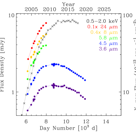
Figure 1: SN 1987A light curves throughout the entire Spitzer mission. The Chandra soft X-ray light curve (0.5-2 keV, Frank et al., 2016) is shown for comparison (black $\times$ symbols).

The 3.6 $\mu$m light curve contains more irregularities in its measurements than the 4.5 $\mu$m light curve. The general trend at 3.6 $\mu$m is similar to that at 4.5 $\mu$m, but the present decline is somewhat slower. However, we caution that the 3.6 $\mu$m flux densities are much more sensitive to any errors in subtraction of the estimated flux densities of Stars 2 and 3, because of the strongly contrasting colors between the SN and the stars.

Given the apparent exponential decay of the 4.5 $\mu$m light curve, a model is suggested in which the emission turns on as the shock sweeps into the ER, and then progressively decays away after the passage of the shock. A very simple form of the model would thus be a gaussian function convolved with an exponential decay as described by

$$S(t) = A\exp[-0.5(t-d_{0})^{2}/\sigma_{\rm d}^{2}]*\exp(-t/\tau_{\rm d})$$

$$= A\int^{\infty}_{-\infty}\exp[-0.5(t^{\prime}-d_{0})^{2}/\sigma_{\rm d}^{2}]\exp[-(t-t^{\prime})/\tau_{\rm d}]dt^{\prime}$$

where $*$ represents convolution. The free parameters of this model are: an amplitude, $A$, which is proportional to the emissivity of the material; a date, $d_{0}$, which sets a nominal date for the peak of the interaction; a time scale for the gaussian function, $\sigma_{\rm d}$, which sets the scale for the rise in the emission; and a time scale for the exponential function, $\tau_{\rm d}$, which sets the scale for the fading. Figure 2 depicts the application of this model to the Spitzer data, Chandra X-ray data (Frank et al., 2016), and Hubble optical data (Larsson et al., 2019). The X-ray data are supplemented with 4 additional epochs of observations (from GO cycles 17 and 18) which were similarly acquired and reduced as described by Frank et al. (2016). At 5.8, 8, and 24 $\mu$m the decay time scale, $\tau_{\rm d}$, was fixed at the value determined at 4.5 $\mu$m because of the lack of late time data.

Figure 2: The Spitzer, soft X-ray (0.5-2 keV, Frank et al., 2016), and optical (Larsson et al., 2019) light curves (black points) fitted with the model of Equation (1) (red line). For reference, the model components are drawn with dotted and dashed lines with an arbitrary normalization. The center ($d_{0}$) and width ($\sigma_{\rm d}$) of the gaussian function are listed, as is the time scale ($\tau_{\rm d}$) for the exponential function. At 5.8 – 24 $\mu$m the parameter $\tau_{\rm d}$ is fixed to the value that is derived at 4.5 $\mu$m. The intensity range shown for the X-ray emission is wider than that of the other wavelengths.

4 High-Resolution Images: Deconvolution and Decomposition

4.1 Deconvolution

The frequently repeated observations of SN 1987A allow mapping the data into finer scale mosaics than the standard pBCD data product. Using data from throughout the mission we have created mosaics with $0.4^{\prime\prime}$ pixel spatial scales (as in Arendt et al., 2016) and $0.2^{\prime\prime}$ pixel spatial scales (Figure 3). With $0.4^{\prime\prime}$ pixels, the ER appears better separated from Stars 2 and 3. On $0.2^{\prime\prime}$ pixels the images become noisier rather than sharper. The increased noise is because the interlacing mapping method leads to very shallow coverage per pixel at this scale. The lack of improved resolution is because the pixels are already sufficiently small that they no longer represent a significant extra convolution of the intrinsic point spread function (PSF) in the final mosaics.

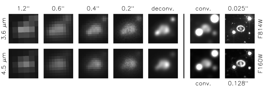
Figure 3: High resolution IRAC imaging the SN 1987A ER. The first column illustrates the SN as seen in a single BCD frame at the intrinsic $1.2^{\prime\prime}$ pixel scale of the detectors. The second column shows a standard pBCD mosaic (generated on $0.6^{\prime\prime}$ pixels) from the observations at one epoch. The third column shows a custom mosaic on $0.4^{\prime\prime}$ pixels generated from data at all epochs. The fourth column is another custom mosaic on $0.2^{\prime\prime}$ pixels, again using data from all epochs. The mosaic with $0.2^{\prime\prime}$ pixels is then deconvolved to provide the images in the 5th column. The appearance of the ER in these images is similar to that in Hubble observations (seventh column) if those observation are convolved to comparable resolution (sixth column). North is up, and east is to the left. The field of view is $6.4^{\prime\prime}\times 6.4^{\prime\prime}$.

However the $0.2^{\prime\prime}$ pixel mosaics are suitable for application of deconvolution techniques. In this study we have processed these mosaics using the IDLASTRO procedure Max_Likelihood (Landsman, 1993), using PSFs generated from the Fourier transform of the idealized Spitzer aperture (outer diameter = 0.85 m, inner diameter = 0.32 m, Werner et al., 2004). A standard IRAC PSF was not used because the data were taken at many different position angles, making the effective PSF azimuthally symmetric. The diffraction features of the three secondary mirror supports are washed out in the effective PSF, and thus omitted in the model PSF. The deconvolved $0.2^{\prime\prime}$ images are shown in Figure 3. In the deconvolved images (especially at 3.6 $\mu$m), the SN is distinct from stars 2 and 3, and the morphology of the emission is seen to be dominated by the ER. The ER appears brighter in the southwest and fainter in the southeast. For comparison, the figure also shows that when convolved to the same resolution, high-resolution Hubble images look similar to the deconvolved IRAC images. The F814W ACS image was taken at Day 6505, near the start of the IRAC observations. The F160W WFC3 image was taken at Day 8718, near the time when the brightness of the ER peaked at 3.6 and 4.5 $\mu$m, and thus it is more similar to the deconvolved image generated from the entire span of the IRAC data. At the shorter wavelengths observed by Hubble, the stars are much brighter relative to the ER.

We find that the deconvolution procedure is insensitive to artificially added noise (at a $1\sigma$ level), but is mildly sensitive to the PSF, producing spurious results if attempted with PSFs that are 50% larger or smaller. The procedure was tried on mosaics with larger ($0.3^{\prime\prime}$ and $0.4^{\prime\prime}$) pixels, but performed less well. We used 10 iterations of the procedure, as there was relatively little improvement in sharpness with more iterations. We found a nearby isolated point source can be fit by a gaussian with full width at half maximum (FWHM) of $1.01^{\prime\prime}$ at both 3.6 and 4.5 $\mu$m. Overall, the effectiveness of deconvolution achieved here is similar to that demonstrated by Velusamy et al. (2008).

4.2 Decomposition

We looked for temporal changes in the ER structure by dividing the data set into three intervals: early, middle, and late epochs. The intervals exclude the earliest data when the emission was rising rapidly, each contain a similar number of observations, and roughly correspond to: the rise to the peak, peak brightness, and decline. When divided this way, the depth of coverage is too low to allow mapping onto $0.2^{\prime\prime}$ pixels and deconvolution. However, mapping on $0.4^{\prime\prime}$ pixel still works well. Images constructed from the early, middle and late epochs are shown in Figure 4. Despite the limited resolution, comparison of the images indicates that the emission was relatively uniformly distributed around the ER at the early epochs. At the middle epochs the ER becomes more asymmetric, being brighter in the southwest. At late epochs the asymmetry becomes more distinct as the southwest fades more slowly than the rest of the ER.

We decompose these $0.4^{\prime\prime}$ images by modeling the emission as the linear combination of 7 components. The first three model components are Stars 2, 3, and 4 (Walker & Suntzeff, 1990). The ER could be represented by several dozen individual knots; however independently solving for the brightness of each knot would lead to degeneracies. Thus, the ER was represented by 4 arcs of knots (or segments), as suggested in Figure 5. Along each of the 4 arcs, the knots are assumed to be of uniform brightness, but the relative brightnesses of each arc are independent. All 7 of these components are convolved with an empirical PSF (for each mosaic) that is taken from a nearby isolated bright star in the image. The convolved components are shown with equal normalization in Figure 5, to show that they do represent spatially distinct components even after convolution.

The model does not fit, or include any adjustment for, the expansion of the ER over time. The expansion rate at X-ray wavelengths from Frank et al. (2016) translates to $0.02^{\prime\prime}$ per 1000 days, or about $0.09^{\prime\prime}$ over the span of the three intervals being modeled. Larsson et al. (2019) report an expansion rate almost 3 times slower from examination of B and R band Hubble images.

A linear regression is used to solve for the amplitudes of each of the model components. The formal uncertainties on the amplitudes are $\lesssim 2\%$. The resulting models are compared to the actual images in Figure 4. The residuals in the difference between the data and the models do not suggest there is any additional component missing from the model. Specifically, there is no indication that a central component representing the slower ejecta is needed.

The brightnesses of the model components at early, middle, and late epochs are plotted in Figure 6. The brightnesses are normalized such that the sum of the 4 ER components is well matched by the integrated 3.6 $\mu$m light curve (Figure 1). There are moderately strong inverse correlations between adjacent ER segments with $0.34<\sigma_{ij}^{2}/\sigma_{i}\sigma_{j}<0.44$, and positive correlations between opposing segments with $0.10<\sigma_{ij}^{2}/\sigma_{i}\sigma_{j}<0.18$. There is also an inverse correlation between the east ER segment and Star 3: $\sigma_{ij}^{2}/\sigma_{i}\sigma_{j}=0.22$. These results indicate that the west segment of the ER has brightened substantially during the span of observations, while the other segments have been fading throughout the observations. This supports and quantifies the apparent asymmetries in the images in Figure 4.

The mapping and decomposition procedures were also applied to the individual epochs of targeted observation without averaging into broader intervals. In this case, $\sim 25\%$ of the $0.4^{\prime\prime}$ pixels in the images contain no data, and the decomposition is applied giving no weight to these pixels. The results are, as expected, much noisier than those illustrated above, but the same trends do emerge when similar averaging is applied after, rather than before, the decomposition.

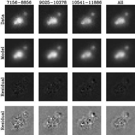
Figure 4: (top row) 3.6 $\mu$m images constructed on $0.4^{\prime\prime}$ pixels at different epochs as indicated by the day number ranges for each figure. The “All” image includes all epochs, and is the same as in Figure 3. With increasing time, the ER emission becomes more asymmetric with the southwest region becoming the brightest portion at late times. Linear scaling from [-1,7] MJy sr^-1. (second row) The corresponding modeled emission at each epoch, displayed on the same scale as the images above. (third row) Difference between data and model, on the same scale. (fourth row) Difference between data and model, displayed with linear scaling from [-1,1] MJy sr^-1. North is up, and east is to the left. The field of view of each panel is $9.6^{\prime\prime}\times 9.6^{\prime\prime}$).

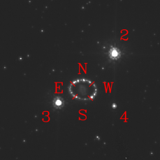
Figure 5: The Hubble image (F814W ACS from Day 6505) in the top panel is used to define the 3.6 $\mu$m emission model’s seven components: Stars 2, 3, and 4, and four segments of the ER. The bottom panel shows these components after convolution with the effective 3.6 $\mu$m PSF and mapped on $0.4^{\prime\prime}$ pixels. For illustration purposes, the components are all normalized to unity and the ER components have been colorized with 4 different colors. The field of view matches that used in Figure 4.

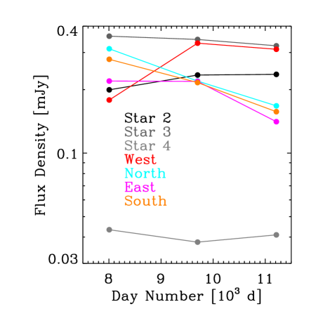
Figure 6: The 3.6 $\mu$m light curves of the four ER segments and the 3 surrounding stars, derived from the decomposition of the $0.4^{\prime\prime}$ mosaics at 3 epochs. Formal uncertainties on the flux densities are $\lesssim 2\%$.

5 Discussion

Across all IR wavelengths, the light curves are reasonably well fitted by the model of Equation (1) with similar parameters (Figure 2). This empirical model is similar in form to those developed by Lundqvist & Fransson (1991) and Dwek & Felten (1992) to explain the prompt line emission from the ER. In those models, the light travel time across the ER (326 d for an ER with radius $R=239$ lt-days and inclination $i=43\arcdeg$ Dwek & Felten, 1992) is explicitly modeled. Here, the light travel delays can be assumed to be a contributing factor to the width of the gaussian component of our model. Irregularities in the radius and density distribution of the ER and asymmetries in the radius (or velocity) of the blast wave would be other contributing factors.

The X-ray light curve is also well fitted by this model, although the date, $d_{0}$, of the peak of the gaussian function is somewhat later, and the exponential time scale, $\tau_{d}$ is significantly longer than at the IR wavelengths. Both these differences act to shift the peak of the X-ray light curve to a later date. In a very simple interpretation, and assuming that the IR emission is from dust that is collisionally heated by the X-ray emitting gas (Dwek, 1986; Bocchio et al., 2013), the shorter exponential time scale for the IR emission compared to that of the X-ray emission, may suggest that dust is being destroyed faster than the gas is cooling. However, additional factors such as the development of a reverse shock, and variations in the density (and consequent post-shock temperature) of the CSM may also contribute to the differences in $d_{0}$ and $\tau_{\rm d}$ between the IR and X-ray light curves. Systematic differences in the IR and X-ray trends that may be indicative of dust destruction had been much more difficult to identify prior to about Day 8000 while both light curves were still rising (e.g. Dwek et al., 2008, 2010).

As shown in Figure 2, we also find that the model of Equation (1) provides a good fit to the evolution of the B, R, and F502N band optical emission reported by Larsson et al. (2019) if restricted to dates after Day 5500 when the interaction with the ER is well developed. Larsson et al. (2019) note that the F502N band (dominated by [O III] line emission) rises and fades more rapidly than the B and R band emission. We find these differences reflected more by the $\tau_{\rm d}$ decay rate of the model’s exponential term, than the $\sigma_{\rm d}$ width of the gaussian term. The model’s parameters for the optical emission are similar to the parameters for the IR emission. Specifically, the decay time scales for the R and B band emission are $\lesssim 30\%$ longer than $\tau_{\rm d}$ at 4.5 $\mu$m, while the decay time scale for the X-ray emission is $>2$ times longer. If the dust is associated with the denser gas clumps that dominate the optical emission rather than the X-ray emitting gas, then there is little evidence from the total ER light curves to indicate ongoing dust destruction. More detailed analysis about the origin and evolution of the dust and the infrared emission from the ER will be addressed in a forthcoming paper (Dwek et al., 2020).

The deconvolution and decomposition provide conclusive evidence that the 3.6 and 4.5 $\mu$m emission is dominated by the ER and not the ejecta. The decomposition also clearly shows that at 3.6 $\mu$m the west side of the ER is brightening relative to the rest of the ER. The behavior is consistent with that observed in the better spatially-resolved and better temporally-sampled X-ray and optical results obtained by Frank et al. (2016) and Larsson et al. (2019). Our first time interval, Days 7156 – 8856, spans the time when both the optical and X-ray emission were transitioning from a brighter eastern side to a brighter western side. During our latter two epochs, we find the west half of the ER is brighter at 3.6 $\mu$m by similar proportions as at X-ray and optical wavelengths.

The 3.6 $\mu$m decomposition results imply that the total stellar flux density to be subtracted from the aperture photometry should be 0.61 mJy, rather than the 0.41 mJy that had been used previously (in Table 1, Figure 1, and previous papers). Use of the larger stellar contribution would steepen the decline of the intensity, yielding $\tau_{\rm d}=5628$ for the model shown in Figure 2. This is closer to, but still larger than, $\tau_{\rm d}=5381$ derived at 4.5 $\mu$m. Any adjustments to the assumed stellar flux densities at longer wavelengths would have less importance because the SN is much redder than the stellar sources. Walborn et al. (1993) identified Star 3 as a Be star, and observed it to fade in the $J$, $H$, and $K$ bands by about one magnitude over an interval of $\sim 1000$ days. Thus it is plausible that the star’s brightness during the period of IRAC observations could be brighter (and less constant) than expected.

6 Summary

We have examined the complete record of Spitzer IRAC observations of SN 1987A which span the period from roughly 6000 to 12000 d after the SN explosion. These data include 3.6 and 4.5 $\mu$m photometry as the supernova’s blast wave has run into and through the pre-existing circumstellar equatorial ring (ER). We find that the mid-IR light curves of the encounter can be well fitted by a model that is the convolution of a gaussian function and an exponential decay. The model is a good fit to the soft X-ray and optical light curves as well. With application of deconvolution procedures we can see that the spatial structure of the 3.6 and 4.5 $\mu$m emission matches the equatorial ring rather than the inner ejecta. By modeling the high-resolution maps of the emission at different epochs, we find that the 3.6 $\mu$m emission has changed from being relatively uniform around the ER to being brighter on the western side.

The true nature of the emission at 3.6 and 4.5 $\mu$m should be made clear with the James Webb Space Telescope (JWST; Gardner et al., 2006), which will have vastly improved angular resolution for distinguishing the true morphology of the emission and distinguishing the CSM from the ejecta and from nearby stars. More importantly, JWST will provide high resolution spectral data across this wavelength regime which will clearly identify line and continuum components, thus revealing the true physical source of the emission.

The Spitzer IRAC observations serendipitously also revealed a strong slow variable object in the same wide field of view as SN 1987A (see Appendix). An optical spectrum obtained for this source indicates that it is a previously unreported Be star.

We thank K. Frank for providing the additional epochs of X-ray data that are presented here, A. Kashlinsky for pointing out the possibility of the variable source being a microlensing event, and E. Pompei for subsequently obtaining the spectrum showing the source is a Be star. We thank the referee for comments that led to improved clarity and content of the work presented here. This work is based on observations made with the Spitzer Space Telescope, which is operated by the Jet Propulsion Laboratory, California Institute of Technology under a contract with NASA. Support for this work was provided by NASA. This research has made use of NASA’s Astrophysics Data System Bibliographic Services. RDG was supported by NASA and the United States Air Force. CEW was supported by NASA.

, Hubble

Appendix

A second strongly variable source

Spitzer has revealed a strongly variable point source that lies just $76^{\prime\prime}$ (PA = $71\arcdeg$) east of SN 1987A, and was thus serendipitously monitored by each of the SN 1987A observations. A 3.6 $\mu$m image of the variable and nearby field stars is shown in Figure 7. Aperture photometry does not yield stable photometry for this source because it is in a crowded field and it is much fainter than SN 1987A. Relative photometry of the variable source and field stars was performed by simultaneous fits of fixed-width gaussian beams to each source, with locations fixed by the source positions in the Hubble Source Catalog (HSC, Whitmore et al., 2016). An initial fit and cross correlation are made to determine any fractional pixel shift in the nominal astrometry. After a positional adjustment, a second fit determines the relative fluxes of each of the sources. The absolute flux densities are set by normalizing the mean intensity of the brightest star (cyan symbols in Figures 7, 8, and 9) to the results given in the Surveying the Agents of Galaxy Evolution (SAGE) Catalog (Meixner et al., 2006). The source flux densities are shown in Figure 8. The light curves demonstrate the good stability of the field stars during a period where the variable source brightens by a factor of $\sim 4$, and almost returns to its original brightness over a span of $\sim 3000$ days. The 5.8 and 8 $\mu$m observations only exist prior to the main outburst. The variable source is not detected at these wavelengths, except for a roughly one year interval centered at modified julian date (MJD) MJD-52500 = 1851 (= 2007 Sep 8) when the source does appear at 5.8 $\mu$m. This matches the much smaller outburst that occurs simultaneously at 3.6 and 4.5 $\mu$m at this time. The serendipitous monitoring with Hubble [Wide Field and Planetary Camera 2 (WFPC2) and Wide Field Camera 3 (WFC3) observations collected in the HSC] mostly misses the strong outburst period, as SN 1987A was usually observed in subarray modes that used insufficiently large fields of view to capture this source. The few observations that do exist suggest that the outburst was fainter or absent at shorter wavelengths. The source is not listed in the Hubble Catalog of Variables (HCV, Bonanos et al., 2019), but is flagged as variable in the Visible and Infrared Survey Telescope for Astronomy (VISTA) Magellanic Clouds survey (VMC DR4, Cioni et al., 2011). Variability information is listed as “NOT$\_$AVAILABLE” in the Gaia DR2 catalog (Gaia Collaboration et al., 2018; Holl et al., 2018).

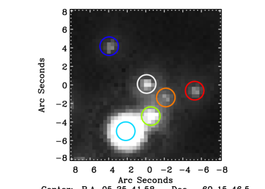
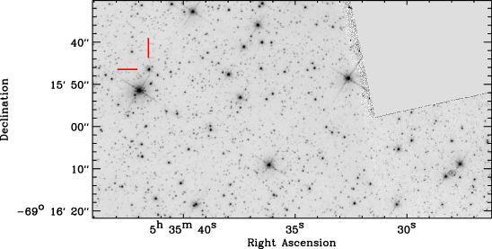
Figure 7: (left) 3.6 $\mu$m image of the variable source (white circle) and surrounding stars that were simultaneously fitted (colored circles). (right) Location of the variable source (red lines) relative to SN 1987A (at lower right) in a WFPC2 F814W image from HST.

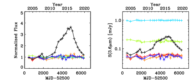
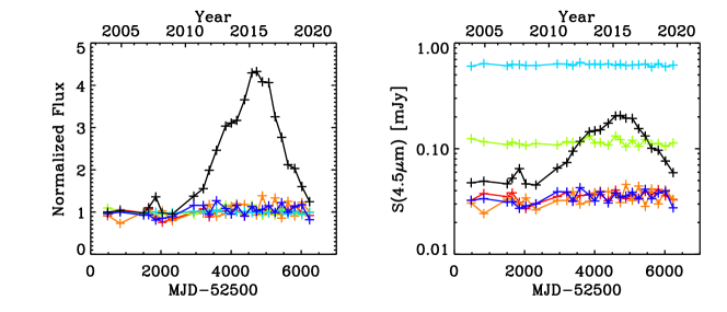
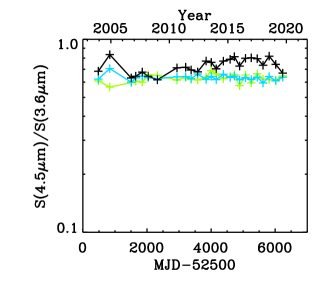
Figure 8: 3.6 $\mu$m (top row) and 4.5 $\mu$m (bottom row) light curves of the sources in Figure 7. In the left column all the light curves are normalized to the respective flux densities at early times. In the middle column, the absolute flux densities are shown. The symbol colors of the stable stars match those used in Figure 7 (left). The panel at lower right shows that color of the variable source steadily changes with respect to the stable colors of the two brighter sources.

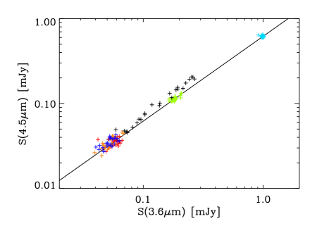
Figure 9: The correlation between the 3.6 and 4.5 $\mu$m fluxes for the sources in Figure 7. The field sources (colored symbols) exhibit a fixed color that is well matched to the Rayleigh-Jeans tail of a blackbody spectrum (trend indicated by the black line). The variable source (black symbols) is close to the blackbody color when faint, but systematically reddens as it brightens.

A possible explanation for this source is that is it a classical Be star. The brightness and colors of the star are generally consistent with a main sequence B star in the LMC. More specifically, the ultraviolet – mid-IR SED is very similar to those of classical Be stars reported by Gehrz et al. (1974) or Bonanos et al. (2009) for example, with excess 3.6 and 4.5 $\mu$m emission attributable to free-free emission. A change in the circumstellar free-free emission could occur with relatively little impact on the brightness at shorter wavelengths. The outburst seems rather large and long for typical Be star behavior, but may represent an extreme example. Classical Be star outbursts usually rise faster than they decline (Rivinius et al., 2013; Labadie-Bartz et al., 2017).

On 2018 Nov 26 (MJD = 58448.2), E. Pompei (private communication) used the European Southern Observatory (ESO) Faint Object Spectrograph and Camera (EFOSC) on the ESO New Technology Telescope (NTT) to obtain a 3600-9200Å spectrum (720 s exposure, $R\sim 500$) of the source. The spectrum confirms that this is a Be star, showing H$\alpha$ in emission. H$\beta$ appears as a weak absorption line, and higher Balmer lines are clearly seen in absorption. Overall, the spectrum closely resembles that of the B3Ve star HD 191610 (Valdes et al., 2004).

The spectrum firmly rules out the alternate possibility that the source is an active galactic nucleus or quasar. Archival Hubble images show no indication of diffuse emission (i.e. a host galaxy) around the variable point source, although there appears to be a background galaxy located $12^{\prime\prime}$ to the northeast.

A third possibility we considered is that this is a gravitational microlensing event. The long duration would imply an exceptionally massive lens, or an exceptionally small transverse velocity. However, the asymmetric light curve (and the smaller earlier brightening) would necessitate complex lens and/or source structures. A larger difficulty with this explanation is that the magnification should be independent of wavelength, while the observations indicate a distinct reddening during the main outburst (Figures 8 and 9).

References

- Arendt et al. (2016) Arendt, R. G., Dwek, E., Bouchet, P., et al. 2016, AJ, 151, 62
- Arendt et al. (2010) Arendt, R. G., Kashlinsky, A., Moseley, S. H., & Mather, J. 2010, ApJS, 186, 10
- Bocchio et al. (2013) Bocchio, M., Jones, A. P., Verstraete, L., et al. 2013, A&A, 556, A6
- Bonanos et al. (2009) Bonanos, A. Z., Massa, D. L., Sewilo, M., et al. 2009, AJ, 138, 1003
- Bonanos et al. (2019) Bonanos, A. Z., Yang, M., Sokolovsky, K. V., et al. 2019, A&A, 630, A92
- Bouchet et al. (2000) Bouchet, P., Lawrence, S., Crotts, A., et al. 2000, IAU Circ., 7354
- Bouchet et al. (2006) Bouchet, P., Dwek, E., Danziger, J., et al. 2006, ApJ, 650, 212
- Cigan et al. (2019) Cigan, P., Matsuura, M., Gomez, H. L., et al. 2019, ApJ, 886, 51
- Cioni et al. (2011) Cioni, M. R. L., Clementini, G., Girardi, L., et al. 2011, A&A, 527, A116
- Crotts et al. (1989) Crotts, A. P. S., Kunkel, W. E., & McCarthy, P. J. 1989, ApJ, 347, L61
- Dwek (1986) Dwek, E. 1986, ApJ, 302, 363
- Dwek & Felten (1992) Dwek, E., & Felten, J. E. 1992, ApJ, 387, 551
- Dwek et al. (2008) Dwek, E., Arendt, R. G., Bouchet, P., et al. 2008, ApJ, 676, 1029
- Dwek et al. (2010) —. 2010, ApJ, 722, 425
- Dwek et al. (2020) Dwek, E., et al. 2020, in preparation
- Fazio et al. (2004) Fazio, G. G., Hora, J. L., Allen, L. E., et al. 2004, ApJS, 154, 10
- Fischera et al. (2002) Fischera, J., Tuffs, R. J., & Völk, H. J. 2002, A&A, 395, 189
- Fixsen et al. (2000) Fixsen, D. J., Moseley, S. H., & Arendt, R. G. 2000, ApJS, 128, 651
- Frank et al. (2016) Frank, K. A., Zhekov, S. A., Park, S., et al. 2016, ApJ, 829, 40
- Fransson et al. (1989) Fransson, C., Cassatella, A., Gilmozzi, R., et al. 1989, ApJ, 336, 429
- Fransson et al. (2015) Fransson, C., Larsson, J., Migotto, K., et al. 2015, ApJ, 806, L19
- Gaia Collaboration et al. (2018) Gaia Collaboration, Brown, A. G. A., Vallenari, A., et al. 2018, A&A, 616, A1
- Gardner et al. (2006) Gardner, J. P., Mather, J. C., Clampin, M., et al. 2006, Space Sci. Rev., 123, 485
- Gehrz et al. (2009) Gehrz, R. D., Becklin, E. E., de Pater, I., et al. 2009, Advances in Space Research, 44, 413
- Gehrz et al. (1974) Gehrz, R. D., Hackwell, J. A., & Jones, T. W. 1974, ApJ, 191, 675
- Gehrz et al. (2007) Gehrz, R. D., Roellig, T. L., Werner, M. W., et al. 2007, Review of Scientific Instruments, 78, 011302
- Herter et al. (2012) Herter, T. L., Adams, J. D., De Buizer, J. M., et al. 2012, ApJ, 749, L18
- Holl et al. (2018) Holl, B., Audard, M., Nienartowicz, K., et al. 2018, A&A, 618, A30
- Houck et al. (2004) Houck, J. R., Roellig, T. L., van Cleve, J., et al. 2004, ApJS, 154, 18
- Indebetouw et al. (2014) Indebetouw, R., Matsuura, M., Dwek, E., et al. 2014, ApJ, 782, L2
- Jakobsen et al. (1991) Jakobsen, P., Albrecht, R., Barbieri, C., et al. 1991, ApJ, 369, L63
- Labadie-Bartz et al. (2017) Labadie-Bartz, J., Pepper, J., McSwain, M. V., et al. 2017, The Astronomical Journal, 153, 252
- Landsman (1993) Landsman, W. B. 1993, in Astronomical Society of the Pacific Conference Series, Vol. 52, Astronomical Data Analysis Software and Systems II, ed. R. J. Hanisch, R. J. V. Brissenden, & J. Barnes, 246
- Landsman (1995) Landsman, W. B. 1995, in Astronomical Society of the Pacific Conference Series, Vol. 77, Astronomical Data Analysis Software and Systems IV, ed. R. A. Shaw, H. E. Payne, & J. J. E. Hayes, 437
- Larsson et al. (2019) Larsson, J., Fransson, C., Alp, D., et al. 2019, ApJ, 886, 147
- Lawrence et al. (2000) Lawrence, S. S., Sugerman, B. E., Bouchet, P., et al. 2000, ApJ, 537, L123
- Lundqvist & Fransson (1991) Lundqvist, P., & Fransson, C. 1991, ApJ, 380, 575
- Luo et al. (1994) Luo, D., McCray, R., & Slavin, J. 1994, ApJ, 430, 264
- Matsuura et al. (2011) Matsuura, M., Dwek, E., Meixner, M., et al. 2011, Science, 333, 1258
- Matsuura et al. (2019) Matsuura, M., De Buizer, J. M., Arendt, R. G., et al. 2019, MNRAS, 482, 1715
- McCray & Fransson (2016) McCray, R., & Fransson, C. 2016, ARA&A, 54, 19
- Meixner et al. (2006) Meixner, M., Gordon, K. D., Indebetouw, R., et al. 2006, AJ, 132, 2268
- Pun et al. (1997) Pun, C. S. J., Sonneborn, G., Bowers, C., et al. 1997, IAU Circ., 6665
- Rieke et al. (2004) Rieke, G. H., Young, E. T., Engelbracht, C. W., et al. 2004, ApJS, 154, 25
- Rivinius et al. (2013) Rivinius, T., Carciofi, A. C., & Martayan, C. 2013, A&A Rev., 21, 69
- Valdes et al. (2004) Valdes, F., Gupta, R., Rose, J. A., Singh, H. P., & Bell, D. J. 2004, ApJS, 152, 251
- Velusamy et al. (2008) Velusamy, T., Marsh, K. A., Beichman, C. A., Backus, C. R., & Thompson, T. J. 2008, AJ, 136, 197
- Walborn et al. (1993) Walborn, N. R., Phillips, M. M., Walker, A. R., & Elias, J. H. 1993, PASP, 105, 1240
- Walker & Suntzeff (1990) Walker, A. R., & Suntzeff, N. B. 1990, PASP, 102, 131
- Wampler et al. (1990) Wampler, E. J., Wang, L., Baade, D., et al. 1990, ApJ, 362, L13
- Werner et al. (2004) Werner, M. W., Roellig, T. L., Low, F. J., et al. 2004, ApJS, 154, 1
- Whitmore et al. (2016) Whitmore, B. C., Allam, S. S., Budavári, T., et al. 2016, AJ, 151, 134
- Young et al. (2012) Young, E. T., Becklin, E. E., Marcum, P. M., et al. 2012, ApJ, 749, L17