Mitigating large adversarial perturbations on X-MAS (X minus Moving Averaged Samples)

Abstract

We propose the scheme that mitigates the adversarial perturbation $\epsilon$ on the adversarial example $X_{adv}$ ($=$ $X$ $\pm$ $\epsilon$, $X$ is a benign sample) by subtracting the estimated perturbation $\hat{\epsilon}$ from $X$ $+$ $\epsilon$ and adding $\hat{\epsilon}$ to $X$ $-$ $\epsilon$. The estimated perturbation $\hat{\epsilon}$ comes from the difference between $X_{adv}$ and its moving-averaged outcome $W_{avg}*X_{adv}$ where $W_{avg}$ is $N\times N$ moving average kernel that all the coefficients are one. Usually, the adjacent samples of an image are close to each other such that we can let $X$ $\approx$ $W_{avg}*X$ (naming this relation after X-MAS[X minus Moving Averaged Samples]). By doing that, we can make the estimated perturbation $\hat{\epsilon}$ falls within the range of $\epsilon$. The scheme is also extended to do the multi-level mitigation by configuring the mitigated adversarial example $X_{adv}$ $\pm$ $\hat{\epsilon}$ as a new adversarial example to be mitigated. The multi-level mitigation gets $X_{adv}$ closer to $X$ with a smaller (i.e. mitigated) perturbation than original unmitigated perturbation by setting the moving averaged adversarial sample $W_{avg}*X_{adv}$ (which has the smaller perturbation than $X_{adv}$ if $X$ $\approx$ $W_{avg}*X$) as the boundary condition that the multi-level mitigation cannot cross over (i.e. decreasing $\epsilon$ cannot go below and increasing $\epsilon$ cannot go beyond). With the multi-level mitigation, we can get high prediction accuracies even in the adversarial example having a large perturbation (i.e. $\epsilon$ $>$ $16$). The proposed scheme is evaluated with adversarial examples crafted by the FGSM (Fast Gradient Sign Method) based attacks on ResNet-50 trained with ImageNet dataset.

1 Introduction

Adversarial perturbations (alexey; cnw; chuan) for a CNN (Convolutional Neural Network) are crafted to make a CNN classifier mispredict its input image. Usually, perturbations are imperceptible to human eyes especially when their size(as known as $\epsilon$)s are small (i.e. $\epsilon$ $\leq$ $16$ in the FGSM [Fast Gradient Sign Method] based attack (alexey)). However, even in the case that an adversarial perturbation on an input image is large ($>$ 16), human beings can classify the image with a correct label.

For the defense of a CNN against the adversarially perturbed images, there have been the approaches (thermometer; countering; distillation; scale) to make neural networks robust against the perturbations. Fundamentally, the approaches need to have a full data set of neural networks for a re-training. Also, there are some other approaches which do not require any modification of neural networks (alexey; gintare; deflecting). The approaches utilize the property that adversarial perturbations tend to exist on a high-frequency region (chuan; yash). Thus, the low-pass image filter (i.e. DCT [Discrete Cosine Transform] or wavelet denoising) deletes the perturbations on a high-frequency region by cutting off high-frequency components. However, they are not so effective for the adversarial example having a large perturbation (gintare).

The image transformations such as DCT and wavelet were developed to make the image with less information (i.e. compressed one with less bits) seemingly have a good quality comparable to original one for human beings. They utilize that human beings are not sensitive to small changes of an image. If the techniques originally developed for the less-sensitive human beings (not for the defense against the adversarial perturbations) can be used to invalidate a relatively small perturbation (i.e. $\epsilon$ $\leq$ $16$), it would be able to nullify a large perturbation if we can make the large perturbation become a smaller one that the image transformation can delete.

For the mitigation of an adversarial perturbation $\epsilon$ of the adversarial example $X_{adv}$ ($=$ $X$ $\pm$ $\epsilon$), we find the estimated perturbation $\hat{\epsilon}$ and add it to $X_{adv}$ in the direction of making $|\epsilon|$ small (i.e. $X_{adv}$ $-$ $\hat{\epsilon}$ for $+$ $\epsilon$, $X_{adv}$ $+$ $\hat{\epsilon}$ for $-$ $\epsilon$). The estimated perturbation comes from the difference between $X_{adv}$ and its moving-averaged outcome $W_{avg}*X_{adv}$ where $W_{avg}$ is $N\times N$ moving average kernel that all the coefficients are one. Since $X$ $\approx$ $W_{avg}*X$ among the adjacent samples of an image, we can make the difference between $X_{adv}$ and $W_{avg}*X_{adv}$ less than $\epsilon$. For a large adversarial perturbation (e.g. $\epsilon$ $>$ $16$), the mitigation scheme is extended to do the multi-level mitigation by configuring the mitigated adversarial example as a new adversarial example to be mitigated further. Also, in order to guarantee that more mitigation steps get the adversarial perturbation smaller, the less perturbed moving averaged sample (i.e. $W_{avg}*X_{adv}$ is closer to $X$ than $X_{adv}$ if $X$ $\approx$ $W_{avg}*X$) is set as the boundary condition that the mitigation by subtraction ($X_{adv}$ $-$ $\hat{\epsilon}$) does not go below and the mitigation by addition ($X_{adv}$ $+$ $\hat{\epsilon}$) does not go beyond.

This paper is organized as follows: Section 2 sets up the function $M(\cdot)$ which mitigates a large perturbation that JPEG encoding cannot nullify. $M(\cdot)$ is dedicated to making the large perturbation small such that JPEG encoding is separated as the soothing function from $M(\cdot)$. In Section 3, the way of estimating perturbation is introduced on X-MAS (i.e. when $X$ $\approx$ $W_{avg}*X$) and it is extended to the multilevel-mitigation for a large perturbation. In the end of the section, the proposed mitigation schemes are built in an algorithm with some relevant parameters. Section LABEL:sec:evaluation evaluates the algorithm with some representing adversarial examples having large perturbations. Finally, Section LABEL:sec:conclusion concludes with the summary of our contribution.

2 Problem Setup

Previous researches (alexey; gintare; chuan; yash) identified that JPEG encoding is able to nullify the impact of the adversarial perturbations on the prediction accuracy of a CNN. When the adversarial example $X_{adv}$ is JPEG-encoded and then fed into a CNN which recognizes the benign version of $X_{adv}$, $X$ as $Y_{true}$,

$$Pr[Y_{true}|X] \approx Pr[Y_{true}|JPEG(X_{adv})],$$

$$X_{adv} =X\pm\epsilon,\;\;\epsilon\geq 0$$

where $Pr[Y_{true}|X]$ is the accuracy that a CNN predicts $X$ as the true label $Y_{true}$ and $\epsilon$ is the adversarial perturbation applied to all the samples of an input image for a CNN. Usually, the relation ”$\approx$” of Equation (LABEL:eqn:jpeg_soothe) works well for the small perturbations but it is not valid for the large perturbations as shown in Figure 1.

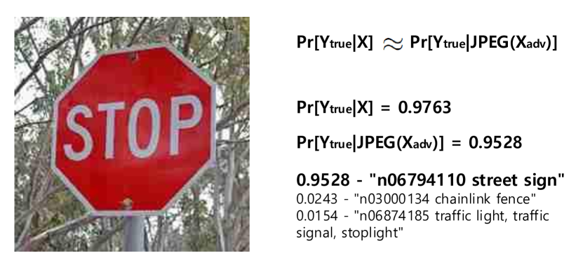
(a) JPEG encoding can well soothe the small perturbations generated by the basic iterative FGSM attack with $\epsilon$ $=$ $2$.

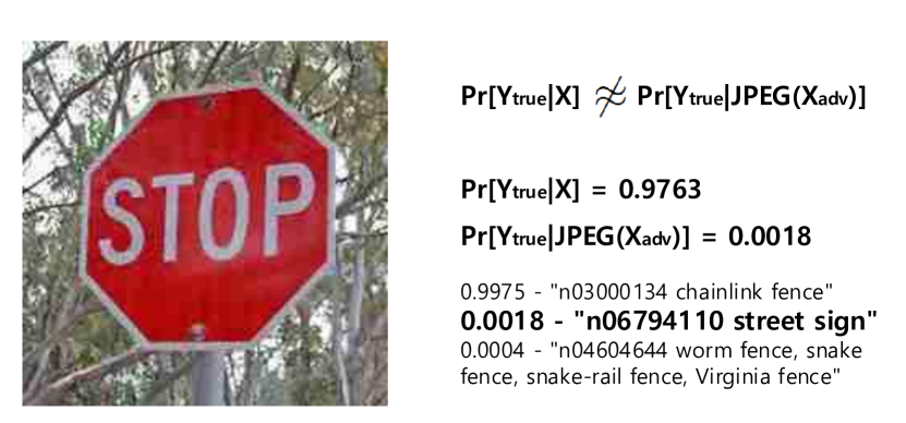
(b) JPEG encoding cannot well soothe the large perturbations crafted by the basic iterative FGSM attack with $\epsilon$ $=$ $32$.

Figure 1: JPEG encoding does not work well for a large perturbation.

In Figure 1, the perturbations $\epsilon$s are crafted by the basic iterative FGSM attack (alexey). Figure 1(a) satisfies the relation ”$\approx$” of Equation (LABEL:eqn:jpeg_soothe) but Figure 1(b) does not. $JPEG(\cdot)$ compresses the image with the quality of 20 (out of 100). In order to make Figure 1(b) have the prediction accuracy comparable to Figure 1(a), we need to mitigate $X_{adv}$ of Figure 1(b) to the level of $X_{adv}$ in Figure 1(a). Let the mitigation function $M(\cdot)$ that mitigates the adversarial perturbation $\epsilon$ of Equation (LABEL:eqn:jpeg_soothe) be

$$M(X_{adv}) =X_{adv}\pm\hat{\epsilon}$$

$$=X\pm\epsilon\mp\hat{\epsilon},\;\;0\leq\hat{\epsilon}\leq\epsilon$$

where $\hat{\epsilon}$ is the estimated perturbation which mitigates the perturbation by subtracting $\hat{\epsilon}$ for $\epsilon$ $>$ 0 and adding $\hat{\epsilon}$ for $\epsilon$ $<$ 0. To make the difference between $M(X_{adv})$ and $X_{adv}$ be imperceptible to human eyes, $\hat{\epsilon}$ must be within the range of $\epsilon$. That is, $\hat{\epsilon}$ should work on the direction of decreasing the range of $\epsilon$ from [$-\epsilon$, $+\epsilon$] to [$-\epsilon$ $+$ $\hat{\epsilon}$, $+\epsilon$ $-$ $\hat{\epsilon}$] where $0$ $\leq$ $\hat{\epsilon}$ $\leq$ $\epsilon$. In Equation (LABEL:eqn:def_miti), $\hat{\epsilon}$ is subtracted for $X_{adv}$ $=$ $X$ $+$ $\epsilon$ and it is added to $X_{adv}$ $=$ $X$ $-$ $\epsilon$. By applying the mitigation function $M(\cdot)$, Equation (LABEL:eqn:jpeg_soothe) can be expressed with the terms as below

$$Pr[Y_{true}|X] \approx Pr[Y_{true}|SF(M(X_{adv}))],$$

$$X_{adv} =X\pm\epsilon,$$

$$M(X_{adv}) =X_{adv}\pm\hat{\epsilon},\;\;0\leq\hat{\epsilon}\leq\epsilon$$

where $SF(\cdot)$ is the soothing function corresponding to JPEG encoding in Equation (LABEL:eqn:jpeg_soothe). Soothing function reduces the impact of the perturbation on the prediction accuracy. As a soothing function, JPEG encoding removes the high-frequency perturbations through DCT (Discrete Cosine Transform) and quantization (chuan; yash). Also, the simple moving average filter (which runs the convolutional computations with the weight kernel where all the coefficients are one) can be used as the soothing function by smoothing the perturbations through the spatial average. In Section 3, we propose the method of estimating $\hat{\epsilon}$ in Equation (LABEL:eqn:def_miti) and the way of mitigating the adversarial perturbation using $\hat{\epsilon}$.

3 Proposed method

3.1 Estimated perturbation $\hat{\epsilon}$

In order to find $\hat{\epsilon}$, we use the moving average filters that make $X_{adv}$ converge some value ranging from [X $-$ $\epsilon$, $X$ $+$ $\epsilon$]. That is,

$$W_{avg}*X_{adv}=W_{avg}*X\pm W_{avg}*\epsilon$$ (4)

where $\epsilon$ $\geq$ $0$ and $W_{avg}$ is $N\times N$ (N $\geq$ 2) moving average window whose samples are convolved with the kernel that all the coefficients are one. The moving average operation ”$W_{avg}*$” decreases the difference between adjacent samples. Thus, the moving-average operation mitigates the perturbation $\epsilon$ as below.

$$W_{avg}*X_{adv}-W_{avg}*X=\pm W_{avg}*\epsilon,$$

$$W_{avg}*|\epsilon|<|\epsilon|\;\;\text{ if }(\frac{1}{|W_{avg}|}\sum_{n=0}^{|W_{avg}|-1}{\epsilon_{n}})\neq\epsilon,$$

$$W_{avg}*\epsilon=\epsilon\;\;\text{ if }(\frac{1}{|W_{avg}|}\sum_{n=0}^{|W_{avg}|-1}{\epsilon_{n}})=\epsilon$$

where $|W_{avg}|$ is the number of coefficients for $N\times N$ $W_{avg}$, $N^{2}$ and $\epsilon_{n}$ is the perturbation assigned to each sample that $W_{avg}$ covers. In Equation(LABEL:eqn:moving_eps), the cases satisfying $W_{avg}*|\epsilon|$ $<$ $|\epsilon|$ are more probable than the cases that meet $W_{avg}*\epsilon$ $=$ $\epsilon$. For example, in order to make $W_{avg}*\epsilon$ $=$ $\epsilon$ in FGSM (Fast Gradient Sign Method) attack (fgsm), all the samples in the coverage of $W_{avg}$ have $\epsilon$. The probability that each sample has the same $\epsilon$ in FGSM is $\frac{1}{3}$ (i.e $+\epsilon$ among $-\epsilon$, 0 and $+\epsilon$). So, the probability that the result of $N\times N$ moving-average computation becomes $\epsilon$ is $\frac{1}{3^{N^{2}}}$. Its value is about $5\times{10}^{-5}$ when $3\times 3$ kernel is used for $W_{avg}$. In the same manner, we can find the probability that the result of $N\times N$ moving-average computation becomes $-\epsilon$ and it is also $\frac{1}{3^{N^{2}}}$. Thus, when $\epsilon$ is generated by the rule of FGSM and the moving average kernel $W_{avg}$ is $3\times 3$, the probability that the inequality $W_{avg}*|\epsilon|$ $<$ $|\epsilon|$ happens is $1$ $-$ $\frac{2}{3^{3^{2}}}$ ($\approx$ 0.9999). Since it is highly probable that $W_{avg}*|\epsilon|$ $<$ $|\epsilon|$, we can use $|\epsilon|$ $-$ $W_{avg}*|\epsilon|$ as the estimated perturbation $\hat{\epsilon}$ in order to make $\epsilon$ smaller. When $X$ $\approx$ $W_{avg}*X$, $\hat{\epsilon}$ can be found by

$$\forall X_{adv} >W_{avg}*X_{adv},$$

$$\hat{\epsilon} =X_{adv}-(W_{avg}*X_{adv})$$

$$=X+\epsilon-W_{avg}*(X+\epsilon)$$

$$\approx\epsilon-W_{avg}*\epsilon\;\;(\because X\approx W_{avg}*X),$$

$$\forall X_{adv} <W_{avg}*X_{adv},$$

$$\hat{\epsilon} =(W_{avg}*X_{adv})-X_{adv}$$

$$=W_{avg}*(X-\epsilon)-(X-\epsilon)$$

$$\approx\epsilon-W_{avg}*\epsilon\;\;(\because X\approx W_{avg}*X)$$

where $\epsilon$ $>$ 0, $X_{adv}$ $=$ $X$ $+$ $\epsilon$ if the moving average output of $X_{adv}$ is smaller than $X_{adv}$ (i.e. $X_{adv}$ $>$ $W_{avg}*X_{adv}$) and $X_{adv}$ $=$ $X$ $-$ $\epsilon$ if the moving average output of $X_{adv}$ is larger than $X_{adv}$ ((i.e. $X_{adv}$ $<$ $W_{avg}*X_{adv}$). $X$ $\approx$ $W_{avg}*X$ can be satisfied by controlling $|W_{avg}|$ (usually, adjacent samples are close to each other).

In Equation (LABEL:eqn:hat_eps), $0$ $<$ $\hat{\epsilon}$ $<$ $\epsilon$ such that $\hat{\epsilon}$ can mitigate $\epsilon$ by either being subtracted from $\epsilon$ or being added to $\epsilon$ That is, when $X_{adv}$ $>$ $W_{avg}*X_{adv}$, $\hat{\epsilon}$ is subtracted from $X_{adv}$ and $\hat{\epsilon}$ is added to $X_{adv}$ if $X_{adv}$ $<$ $W_{avg}*X_{adv}$. Figure 2 illustrates how $\hat{\epsilon}$ mitigates $\epsilon$.

Figure 2: Illustration of mitigating $\epsilon$ with $\hat{\epsilon}$

In Figure 2, the solid black line shows the upper and lower limits where the adversarial perturbation $\epsilon$ works on $X$. Thus, the red line which denotes the adversarial example $X_{adv}$ having $\pm\epsilon$ as the adversarial perturbation, does not get out of the black line. Also, the solid green line indicates the upper and lower boundaries that $\hat{\epsilon}$ works on $X_{adv}$. If ($X$ $+$ $\epsilon$ $-$ $\hat{\epsilon}$) $<$ $X_{adv}$ $<$ ($X$ $+$ $\epsilon$), $X_{adv}$ has the positive $\epsilon$ such that $\hat{\epsilon}$ ($=$ $\epsilon$ $-$ $W_{avg}*\epsilon$) should be subtracted from $X_{adv}$ to reduce $+\epsilon$. On the other hand, if ($X$ $-$ $\epsilon$) $<$ $X_{adv}$ $<$ ($X$ $-$ $\epsilon$ $+$ $\hat{\epsilon}$), $X_{adv}$ has the negative $\epsilon$. Thus, $\hat{\epsilon}$ should be added into $X_{adv}$ to increase $-\epsilon$. Both $X_{adv}$ $+$ $\hat{\epsilon}$ and $X_{adv}$ $-$ $\hat{\epsilon}$ are closer to $X$ than $X$ $+$ $\epsilon$ and $X$ $-$ $\epsilon$ are. In the same manner with $X_{adv}$, the solid blue line that represents the adversarial example $X_{adv}^{1}$ having $\pm(\epsilon-\hat{\epsilon})$ as the adversarial perturbation, does not get out of the green line. If $\hat{\epsilon}$ $=$ 0 (i.e. $X_{adv}$ $=$ $W_{avg}*X_{adv}$), all the samples within the coverage of $W_{avg}$ have the same $\epsilon$. As discussed earlier, the probability that all the samples have the same $\epsilon$ is very low even in the small $3\times 3$ $W_{avg}$. It is much smaller than the probability that $\epsilon$ of $X_{adv}$ is 0 (e.g. $\frac{1}{3}$ in the FGSM based attack). Thus, when $\hat{\epsilon}$ $=$ 0, it is more probable that the perturbation of $X_{adv}$ is zero rather than that all the samples have the same $\epsilon$. Since we do not have to find $\hat{\epsilon}$ for the sample having no perturbation, we do not change $X_{adv}$ in case that $\hat{\epsilon}$ $=$ 0.

In Equation (LABEL:eqn:hat_eps), $\hat{\epsilon}$ can be larger than $\epsilon$ if $X$ $\not\approx$ $W_{avg}*X$. It is the case that samples within the moving average kernel are very different to each other. Then, $\hat{\epsilon}$ may work as another perturbation. Also, $\hat{\epsilon}$ can be too small to improve the prediction accuracy $Pr[Y_{true}|(X_{adv}\pm\hat{\epsilon})]$. For both large and small $\hat{\epsilon}$, more mitigation steps would be required. Figure 3 shows the impact of the single-level mitigation on the prediction accuracy according to the sizes of $\epsilon$ in $X_{adv}$.

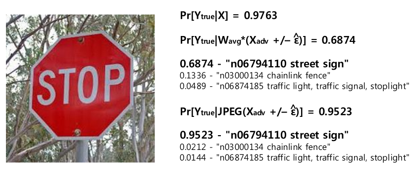
(a) Single-level mitigation can well mitigate the small perturbations crafted by the basic iterative FGSM attack with $\epsilon$ $=$ $2$.

(b) Single-level mitigation may not work well on large perturbations crafted by the basic iterative FGSM attack with $\epsilon$ $=$ $32$.

Figure 3: Impact of the single-level mitigation on the prediction accuracy according to the sizes of $\epsilon$ in $X_{adv}$

In Figure 3, $|W_{avg}|$ $=$ $3$ $\times$ $3$ for both $\hat{\epsilon}$ and the soothing filter ”$W_{avg}*$” of $Pr[Y_{true}|W_{avg}*(X_{adv}+/-\hat{\epsilon})]$. $JPEG(\cdot)$ compresses the image in the quality with 20 (out of 100). Figure 3(a) shows the case where single-level mitigation works very well on the small perturbations to get the high prediction accuracy. However, the single-level mitigation is not so effective on the large perturbation in Figure 3(b). In order to achieve a high prediction accuracy on the adversarial example having large perturbations, we need to run a multi-level mitigation in a controlled manner.

3.2 Multi-level mitigation

The single-level mitigation with the estimated perturbation $\hat{\epsilon}$ in Equation (LABEL:eqn:hat_eps) makes a new adversarial example $X_{adv}^{1}$ that ranges ($X_{adv}$ $+$ $\hat{\epsilon}_{0}$, $X_{adv}$ $-$ $\hat{\epsilon}_{0}$) where $X_{adv}$ for the lower boundary is $X$ $-$ $\epsilon$, $X_{adv}$ for the upper limit is $X$ $+$ $\epsilon$ and $\hat{\epsilon}_{0}$ is $\hat{\epsilon}$ of Equation (LABEL:eqn:hat_eps). In order to find the upper and lower boundaries for $X_{adv}^{2}$ which is mitigated from $X_{adv}^{1}$, we need to estimate the perturbation $\hat{\epsilon}_{1}$ at both ends of the range for $X_{adv}^{1}$.

$$\forall X_{adv} -\hat{\epsilon}_{0},$$

$$\hat{\epsilon}_{1} =(X_{adv}-\hat{\epsilon}_{0})-W_{avg}*(X_{adv}-\hat{\epsilon}_{0})$$

$$=(X+\epsilon-\hat{\epsilon}_{0})-W_{avg}*(X+\epsilon-\hat{\epsilon}_{0})$$

$$\approx\epsilon-\hat{\epsilon}_{0}-W_{avg}*(\epsilon-\hat{\epsilon}_{0})\;\;(\because X\approx W_{avg}*X),$$

$$\forall X_{adv} +\hat{\epsilon}_{0},$$

$$\hat{\epsilon}_{1} =W_{avg}*(X_{adv}+\hat{\epsilon}_{0})-(X_{adv}+\hat{\epsilon}_{0})$$

$$=W_{avg}*(X-\epsilon+\hat{\epsilon}_{0})-(X-\epsilon+\hat{\epsilon}_{0})$$

$$\approx\epsilon-\hat{\epsilon}_{0}-W_{avg}*(\epsilon-\hat{\epsilon}_{0})\;\;(\because X\approx W_{avg}*X)$$

where $\hat{\epsilon}_{0}$ $=$ $\epsilon$ $-$ $W_{avg}*\epsilon$ such that

$$\hat{\epsilon}_{1} =W_{avg}*(\epsilon-W_{avg}*\epsilon)$$

$$=W_{avg}*\hat{\epsilon}_{0}.$$

Since it is more probable that $W_{avg}*|\hat{\epsilon}_{0}|$ $<$ $|\hat{\epsilon}_{0}|$, $|\hat{\epsilon}_{1}|$ $<$ $|\hat{\epsilon}_{0}|$. Thus, $|\hat{\epsilon}_{1}|$ $<$ $|\hat{\epsilon}_{0}|$ $<$ $|\epsilon|$ since $|\hat{\epsilon}_{0}|$ $<$ $|\epsilon|$. Figure 4 illustrates the multi-level mitigation that estimates $\hat{\epsilon}_{1}$.

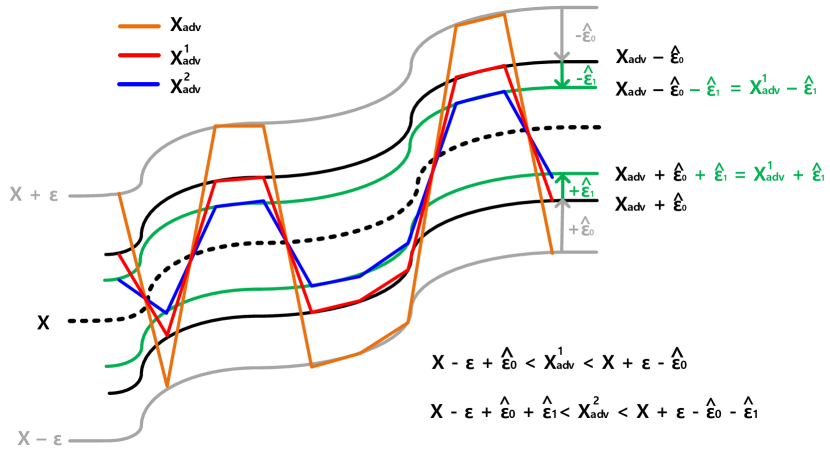
Figure 4: Illustration of the multi-level mitigation

In Figure 4, the grey line is the boundary condition for $X_{adv}$ (corresponding to the solid black line of Figure 2), the solid black line denotes the range of $X_{adv}^{1}$ and the green line represents the upper and lower boundaries that $X_{adv}^{2}$ can reach. As the level of mitigation goes deep, the accumulated sum of the estimated perturbations grows even though the estimated perturbation per each level decreases. Therefore, we should control $\hat{\epsilon}$ to satisfy the following.

$$\sum_{n=0}^{p}|\hat{\epsilon}_{n}| <|\epsilon|\;\;,\;\;|\hat{\epsilon}_{p}|<\cdots<|\hat{\epsilon}_{1}|<|\hat{\epsilon}_{0}|<|\epsilon|$$ (7)

where $p$ is the level of mitigation. However, in Equation (7), $\epsilon$ cannot be directly handled as a single term because it is hidden in $X_{adv}$. In order to control $\hat{\epsilon}$, Equation (7) should be rephrased as below.

$$X+\epsilon-\hat{\epsilon}_{0}-\hat{\epsilon}_{1}\cdots-\hat{\epsilon}_{p-1}-\hat{\epsilon}_{p} >X-\epsilon,$$

$$X-\epsilon+\hat{\epsilon}_{0}+\hat{\epsilon}_{1}\cdots+\hat{\epsilon}_{p-1}+\hat{\epsilon}_{p} <X+\epsilon.$$ (8)

In case that adjacent samples are very different to each other, $X$ $\not\approx$ $W_{avg}*X$ such that the estimated perturbation at the $p$-th step of the multi-level mitigation, $\hat{\epsilon}_{p}$ can be too large to satisfy Equation (8). Since usually $X$ $>$ $\epsilon$, the large difference that breaks the relation of Equation (8) may come from the difference between the benign parts (i.e. $X$ of $X_{adv}$). To relax the impact of the large differences on the estimated perturbations, we normalize the estimated perturbation at the $p$-th step of the multi-level mitigation as below.

$$\hat{\epsilon}_{p} =E[|X_{adv}^{p}-(W_{avg}*X_{adv}^{p})|]$$ (9)

where $E[|\cdot|]$ indicates both $E[X_{adv}^{p}-(W_{avg}*X_{adv}^{p})]$ (to be subtracted from $X_{adv}^{p-1}$) and $E[(W_{avg}*X_{adv}^{p})-X_{adv}^{p}]$ (to be added into $X_{adv}^{p-1}$). This normalization also prevents $\hat{\epsilon}_{p}$ from working as a serious perturbation for $X_{adv}$ having $\epsilon$ $=$ $0$ ($\because$ the mitigation scheme should work for the benign example).

In Equation(8), the boundary condition for both decreasing perturbation $X_{adv}^{p-1}$ $-$ $\hat{\epsilon}$ and increasing perturbation $X_{adv}^{p-1}$ $+$ $\hat{\epsilon}$ better be replaced with the value closer to $X$. As discussed earlier with Equation (LABEL:eqn:moving_eps), the probability for $W_{avg}*|\epsilon|$ $<$ $|\epsilon|$ is much larger than $W_{avg}*|\epsilon|$ $=$ $|\epsilon|$ such that it is more probable that $W_{avg}*X_{adv}$ is closer to $X$ than $X$ $\pm$ $\epsilon$ when $W_{avg}*X$ $\approx$ $X$. That is,

$$\forall X_{adv} =X+\epsilon,$$

$$W_{avg}*X_{adv} =W_{avg}*(X+\epsilon)$$

$$=X+W_{avg}*\epsilon\;\;(\because W_{avg}*X\approx X)$$

$$<X+\epsilon\;\;(\because W_{avg}*|\epsilon|<|\epsilon|),$$

$$\forall X_{adv} =X-\epsilon,$$

$$W_{avg}*X_{adv} =W_{avg}*(X-\epsilon)$$

$$=X-W_{avg}*\epsilon\;\;(\because W_{avg}*X\approx X)$$

$$>X-\epsilon\;\;(\because W_{avg}*|\epsilon|<|\epsilon|).$$

Thus, both $X$ $-$ $\epsilon$ and $X$ $+$ $\epsilon$ of Equation (8) can be replaced with $W_{avg}*X_{adv}$ as following.

$$X_{adv}^{p-1}-\hat{\epsilon}_{p} >W_{avg}*X_{adv},$$

$$X_{adv}^{p-1}+\hat{\epsilon}_{p} <W_{avg}*X_{adv}.$$ (10)

Equation (10) guarantees that the proposed multi-level mitigation gets $X_{adv}$ closer to $X$ with the smaller (i.e. mitigated) perturbation having the same polarity with the original (i.e. unmitigated) perturbation if $X$ $\approx$ $W_{avg}*X$. That is, the term of decreasing $\epsilon$, $X_{adv}^{p-1}$ $-$ $\hat{\epsilon}_{p}$ does not go below $W_{avg}*X_{adv}$ and the term of increasing $\epsilon$, $X_{adv}^{p-1}$ $+$ $\hat{\epsilon}_{p}$ does not go beyond $W_{avg}*X_{adv}$. To this end, $W_{avg}*X_{adv}$ can be used as the decision boundary that determines the maximum mitigation step where the prediction accuracy does not change any longer. Figure 5 shows that the 70-step multi-level mitigation satisfying Equation (10) is applied to the adversarial example having $\epsilon$ $=$ 32 of Figure 3.

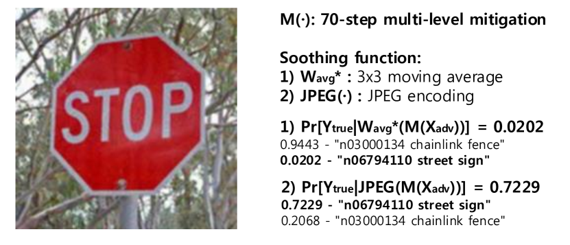
(a) 70-step multi-level mitigation gets higher prediction accuracy than the single-level mitigation of Figure 3(b).

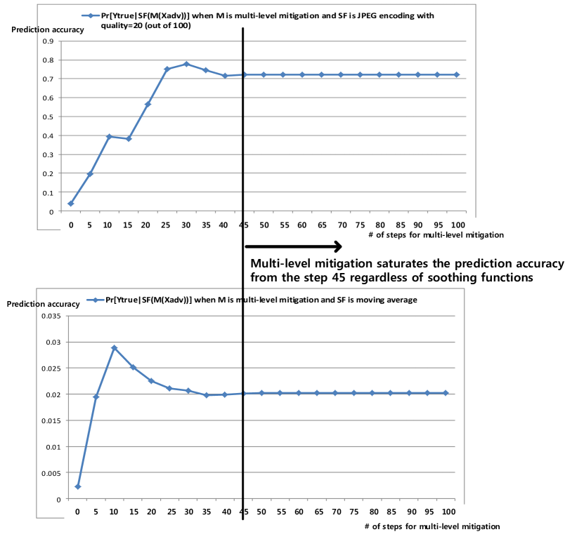
(b) The boundary condition, Equation (10) for multi-level mitigation guarantees a certain level of the enhanced prediction regardless of soothing functions.

Figure 5: The proposed multi-level mitigation enhances the prediction accuracy of Figure 3(b) in a controlled manner.

In Figure 5, even though the prediction accuracies of Figure 5(a) are different according to soothing filters, the mitigation step where their prediction accuracies do not change any longer is same as shown in Figure 5(b). This means that the boundary conditions of Equation (10) guarantee a certain level of prediction accuracy if the number of mitigation steps are large enough like the 70-step multi-level mitigation of Figure 5. Thanks to Equation (10), we can build the algorithmic state machine having the point where the multi-level mitigation stops at.

3.3 Algorithm

Algorithm 1 summarizes the proposed method of mitigating adversarial perturbations.

Algorithm 1 Mitigating adversarial perturbations

//$X_{adv}$is the adversarial example. //$\hat{\epsilon}$is the estimated perturbation. //$W_{avg}$is $N\times N$moving average kernel. //$X_{adv}^{j}$is the adversarial example at the j-th step mitigation //$\hat{\epsilon}_{j}$is the estimated perturbation at the j-step mitigation //$W_{avg}*X_{adv}$is the local expectation that $W_{avg}$covers. //$k$is the size of an array having CNN inference results from $X_{adv}^{j-(k-1)}$to $X_{adv}^{j}$//$SF$is the soothing filter like JPEG encoding //CNN is a convolutional neural network Input:$X_{adv}$, $W_{avg}$, k, SF, CNN //initial step j is set to zero j = 0; //initialize the variable that counts the number of consecutive k-steps //whose prediction accuracies are same equal_count = 0; $X_{adv}^{j}$$\geq$($W_{avg}*X_{adv}^{j}$) //Find $\hat{\epsilon}_{j}$to be subtracted from $X_{adv}^{j-1}$$\hat{\epsilon}_{j}$$=$$X_{adv}^{j}$$-$($W_{avg}*X_{adv}^{j}$); //Mitigate the perturbation with $\hat{\epsilon}_{j}$iff $\hat{\epsilon}_{j}$$\leq$$\hat{\epsilon}_{j-1}$(j $>$0 ) && ( $\hat{\epsilon}_{j}$$\leq$$\hat{\epsilon}_{j-1}$) //Subtract $\hat{\epsilon}_{j}$from $X_{adv}^{j-1}$//if and only if this subtraction meets Equation () ($X_{adv}^{j-1}$$-$$\hat{\epsilon}_{j}$) $>$$W_{avg}*X_{adv}$