One Point, One Object:
Simultaneous 3D Object Segmentation and 6-DOF Pose Estimation

Abstract

We propose a single-shot method for simultaneous 3D object segmentation and 6-DOF pose estimation in pure 3D point clouds scenes based on a consensus that one point only belongs to one object, i.e., each point has the potential power to predict the 6-DOF pose of its corresponding object. Unlike the recently proposed methods of the similar task, which rely on 2D detectors to predict the projection of 3D corners of the 3D bounding boxes and the 6-DOF pose must be estimated by a PnP like spatial transformation method, ours is concise enough not to require additional spatial transformation between different dimensions. Due to the lack of training data for many objects, the recently proposed 2D detection methods try to generate training data by using rendering engine and achieve good results. However, rendering in 3D space along with 6-DOF is relatively difficult. Therefore, we propose an augmented reality technology to generate the training data in semi-virtual reality 3D space. The key component of our method is a multi-task CNN architecture that can simultaneously predicts the 3D object segmentation and 6-DOF pose estimation in pure 3D point clouds.

For experimental evaluation, we generate expanded training data for two state-of-the-arts 3D object datasets [1][2] by using Augmented Reality technology (AR). We evaluate our proposed method on the two datasets. The results show that our method can be well generalized into multiple scenarios and provide performance comparable to or better than the state-of-the-arts.

1 INTRODUCTION

3D object recognition needs to simultaneously detect the given object in a scene and estimate its accurate 6-DOF pose, which plays a key role to many techniques and practical applications, e.g., robotic manipulation, object modeling and scene understanding [3, 4, 5, 6, 7]. The current methods to this task can be divided into the Feature matching methods and the CNN-based prediction methods. In general, Feature matching methods need to generate appropriate features according to the attributes of the given set of object views to build the model database and then match against the scene features. Features can either be the handcrafted features to represent the object surface (texture or surface variation) [8, 2, 1] or, more recently, the learning based features [9, 10, 11]. The performance of such methods mainly depends on the discriminating features and the coverage of the 6-DOF pose space in terms of viewpoint and scale, which increases the running times linearly. In addition, a multi-stage hypothesis verification process is adopted inevitably to refine the hypothesis.

Figure 1: Our method directly processes the original point clouds scene and can simultaneously predicts point-wise segmentation and 6-DOF pose estimation. (A) The input point clouds scene, (B) the point-wise segmentation, (C) the results of the 6-DOF pose estimation with 3D bounding boxes.

Recently, prediction methods based on deep convolution networks are proposed to address these limitations. Instead of using the feature matching engineering, these methods convert the distribution of the whole space of 6-DOF pose into a set of network weights based on a large amount of training datasets, thus eliminating the linear running time. Given that 2D RGB images provide detailed and clear texture information, methods [12, 13, 14, 15] can infer the corners projection of 3D bounding boxes from RGB images. However, the performance of image-based 3D recognition methods are bounded by the accuracy of the spatial mapping. 3D point clouds CNN-based methods [16, 17, 18] usually utilize a voxel grid representation to overcome the irregular structure of point clouds by encoding each voxel that are derived from all the points contained within the voxel. This, however, unnecessary computational complexity and memory consumption of the structure conversion are introduced.

In this paper, we present an efficient single shot method for simultaneously segmenting an object in pure 3D point clouds scenes and predicting its 6-DOF pose without any complicated structure conversion and post-processing for spatial mapping. For 3D point clouds representation, such data is often converted into regular 3D voxel grids, which introduces the voluminous and geometric information loss unnecessarily. Based on a simple consensus that one point only belongs to one object, for a given point clouds scene, each point in the scene has the potential power to predict the 6-DOF pose of its corresponding object. The key component of our method is the process of multi-task segmentation and pose estimation as shown in Fig. 1, which can simultaneously predicts: 1) the point-wise segmentation for filtering out background points and reducing search space, 2) the coordinates of the object 3D bounding box corners for estimating 6-DOF pose transformation and 3) the confidence for evaluating the accuracy of 3D bounding box prediction.

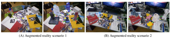
Figure 2: The Augmented Reality technology can be used to quickly create 3D object recognition datasets in fixed working scenarios. (A) the generated AR scenario for Tejani et al. dataset [1], (B) the generated AR scenario for Hinterstoisser et al. dataset [2].

In addition, as shown in Fig. 2, we design an efficient dataset generation method based on Augmented Reality technology (AR) and construct expanded training datas for two state-of-the-arts datasets, i.e., Tejani et al. dataset [1] and Hinterstoisser et al. dataset [2]. To demonstrate the performance of the proposed method, comparison experiments on these two public datasets are performed. In summary, our main contributions are:

• We present a concise enough method for simultaneous 3D object segmentation and 6-DOF pose estimation, which can operate at pure 3D point clouds without any structure conversion and stepwise post-processing.

• We design an efficient dataset generation method for 3D object recognition based on Augmented Reality technology (AR), which can be used to quickly construct 3D object recognition datasets in fixed working scenarios.

• We present extensive experiments to validate the effectiveness of our method using two public datasets, where ours delivers comparable or surpass performance with the state-of-the-arts.

2 RELATED WORKS

We present the main methods of 3D object recognition at present. Generally, these methods can be roughly introduced from (1) Feature matching methods to (2) CNN-based prediction methods.

Feature matching methods. Such methods can be divided into handcrafted features and learning features, which the performance is mainly depending on the discriminating features and the coverage of the 6-DOF pose space in terms of viewpoint and scale. 1) The handcrafted features, like the 2D local features [19, 20, 21], which are extracted from the 2D RGB image and then back projected to real 3D space. This kind of methods performs well on textured objects but suffer from texture-less. 3D local features [22, 23, 24, 25, 26] are generated according to the distribution statistics of the local geometric information on the surface of the object. These methods can handle texture-less objects, but are limited to objects with rich variations of the surface normal. Template features [2, 27, 28] are usually acquired from the object scanning under multiple viewpoint and scale, which is suitable for texture-less objects. Linemod [2] achieves efficient sliding window search on RGBD images, which depends on its fusion of quantized image contours and normal orientations, and innovative use of linear memory characteristics to improve matching speed. Based on the Linemod feature, [28] proposes a hashing strategy to further speed up template matching. 2) The learning features. In order to solve the problem of low discrimination of manually designed features, Doumanoglou et al. [9] proposed using unsupervised Sparse Autoencoder to learn image patch features, and then combined with Hough voting strategy to estimate the object pose. W. Kehl et al. [10] further uses Convolutional Autoencoder to extract patch features, and achieves better results. In order to make full use of 3D spatial geometry information, Liu et al. [11] voxelized the point clouds and proposed a 3D Convolution Autoencoder for feature extraction.

CNN-based prediction methods. Recently, CNN-based methods have gradually been used to solve these limitations [13][14][15]. SSD-6D [13] as a pipeline focus on the object detection relies on the SSD architecture [29], which can simultaneously predicts 2D bounding boxes with the object class. This is followed by an post-processing to transform 2D bounding boxes to 6-DOF pose hypotheses. BB8 [14] is a two-step 3D bounding box detection pipeline, which firstly segments the object in 2D image and then predicts the 2D projection coordinates of the object 3D bounding box for the given segmentation. The 6-DOF pose is calculated by using the PnP algorithm [30]. Seamless [15] is a distinct framework that relies on the backbone of YOLO [31] to predict the 2D projections of the vertices of the object 3D bounding box directly, which are then transform to 6-DOF pose using the PnP algorithm. Most of the above methods can not directly acquire the 6-DOF pose in 3D space of the objects but need a processing of PnP like spatial mapping. Several point clouds [16, 17, 18] based 3D object recognition methods utilize a voxel grid representation to overcome its irregular structure. This, however, structure conversion unnecessarily voluminous and causes issues.

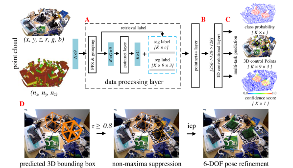
Figure 3: The framework of our simultaneous 3D object segmentation and 6-DOF pose estimation method. For a given 3D point clouds scenes with multiple attributes, we A) sampling/grouping the input scene and generate low density and high dimensional feature data, B) enable to learn point-wise local features, C) predict the point-wise class probability, 3D control points of object 3D bounding boxes and the confidence score, D) refine the prediction via non-maxima suppression and Iterative Closest Point (ICP) [32].

3 APPROACH

As shown in Fig. 3, the goal of our method is to design an end-to-end trainable network, which can output multi-task predictions for simultaneous 3D object segmentation and 6-DOF pose estimation without any structure conversion and stepwise post-processing. The architecture of ours is motivated by Pointnet/Pointnet++ [33][34], which are originally designed to be a single-task classification network that can enable to learn point-wise local features. We design our network to simultaneously predict the point-wise segmentation and the 3D corners of the 3D bounding box around the objects. Then given the point-wise segmentation and the 3D bounding box corners, the invalid 3D corners are filtered out accurately, and the 6-DOF pose can be calculated directly without using any PnP [30] like spatial transformation methods. Now, we describe our network architecture and explain all aspects of our method in details.

3.1 Multi-task Predictions

We formulate the 3D object recognition problem in terms of predicting the point-wise segmentation and 3D control points associated with the 3D models of our objects of interest. Given the 3D coordinate predictions, we filter the invalid coordinate prediction using the segmentation results and directly calculate the object’s 6-DOF pose by the remaining 3D control points. The 3D model of each object is parameterized with 9 control points. 8 of the 9 control points are the corners of the tight 3D bounding box that are fitted to the 3D model. In addition, the 9th point is selected as the the centroid of the object 3D model similar to [15]. This parameterization is general and can be used for any rigid 3D object with arbitrary shape and topology.

As shown in Fig. 3, our model takes as input an expended point clouds data with a size of $N\times 9$, which is represented as a set of 3D points $\{P_{i}|i=1,...,n\}$, where each point $P_{i}$ is a vector of its $(x,y,z)$ coordinate plus extra feature channels, e.g., color $(r,g,b)$ and normal $(n_{x},n_{y},n_{z})$. For the multi-task model, the network will output $[\underline{K}\times(\underline{9}\times 3+\underline{c}+\underline{1})]$ scores for each of the $\underline{K}$ key-points, consisting of predicted 3D coordinates of the $\underline{9}$ control points, the $\underline{c}$ class probabilities and $\underline{1}$ overall confidence score. At test time, predictions at points with negative categories and low confidence scores, i.e. where the valid key points are not present, will be pruned.

Figure 4: We show the distribution of key points obtained by different sampling methods, where the sampling density is 4096 points. (A) The input input point clouds. (B) The result of the Farthest Point Sampling (FPS). (C) The result of the Random Sampling method (RS). FPS can still retain more uniform points in the handle part of the milk model compared with RS method.

The input point clouds data for our network with a size of $N\times 9$ need to be pre-processed as visualized in Fig. 3 (A). Typically, more than 30k points can be obtained using low-cost depth sensors. Because the density of point clouds varies greatly in the whole space, if all points are directly used as the key points, which not only increases the burden of memory/efficiency, but also disturb the accuracy. For this, we use the iterative farthest point sampling (FPS) [35] to choose $K$ subset of the most distant points from the input set. As shown in Fig. 4, the FPS [35] method covers the entire surface shape better comparing with Random Sampling [36]. It is intuitive to see that FPS can still retain more uniform points in the slender parts of the object when comparing with RS method, e.g., the handle of the milk model. At the same time, in order to reduce the loss of local spatial information caused by sampling, each key point will be assigned a local group, where the group corresponds to a local region and $G$ is the number of points in the neighborhood of key points. After the FPS & Grouping, the size of data is transformed to $K\times G\times 9$. Then, a pointnet layer[33] is used as the feature learning block, which can capture local features for each key point. The output data size is $K\times C$ with a new feature dimension of $C$. To train the network, the 3D bounding box of the object needs to be known, which provides the coordinates of 9 control points for points regression. In addition, the point-wise class label is provided for segmentation.

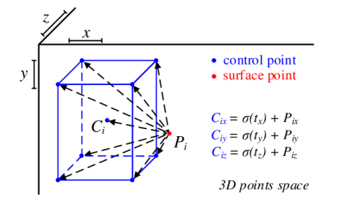
Figure 5: 3D control points prediction. We predict the control point coordinates of the 3D box as offsets from the surface points using a linear activation function $\sigma(x)$.

As shown in Fig. 5, the network predict the control point coordinates of the 3D box as offsets from the surface points using a linear activation function $\sigma(x)=x$. The ground truth value can be easily computed by inverting the equations in Fig. 5, where the ground truth for control points regression correspond to Eq. 1:

$$t_{x}=C_{x}-P_{x}$$ (1)

$$t_{y}=C_{y}-P_{y}$$

$$t_{z}=C_{z}-P_{z}$$

The input data with a size of $N\times 9$ is aligned $[N\times 9\times 3]$ control point coordinates, but valid for only positive class, and $[N\times c]$ class labels. Because the FPS & Grouping layer does not change the spatial information of the point, the key-points ground truth label can be easily retrieved from the original data, where the size is $[K\times(9\times 3+c)]$.

Given the pre-processed training data along with ground truth labels as shown in Fig. 3 (B&C), we use the basic feature layers of Pointnet++ [34] framework concatenated with three 1D convolutional layers to acquire the final key-points features of three branches for point-wise segmentation, control points regression and confidence prediction.

3.2 Training Procedure

The composition of the multi-task loss for training the three branches can be denoted as Eq. 2:

$$\begin{split}\mathcal{L}&=\lambda_{seg}\mathcal{L}_{seg}(p,p^{*})+\lambda_{reg}p^{*}\mathcal{L}_{reg}(x,x^{*})\\ &+\lambda_{conf}p^{*}\mathcal{L}_{conf}\end{split}$$ (2)

Here, the terms of $\mathcal{L}_{seg}(p,p^{*})$ represents the segmentation loss, $p$ and $p^{*}$ are the predicted class probability and ground-truth label respectively, which is trained by cross entropy loss. Specifically, we do a binary classification due to all of the used datasets include single class objects in each testing scene. The terms of $p^{*}\mathcal{L}_{reg}(x,x^{*})$ represents the regression loss of the control points, $p^{*}$ here means the regression loss is activated only for positive class. We use SmoothL1 loss to train the regression. The term of $p^{*}\mathcal{L}_{conf}$ represents the confidence loss for evaluating the accuracy of the control points prediction. The confidence loss is only valid for positive class, where the confidence score function is denoted as Eq. 3:

$$\mathcal{C}_{score}(x)=\begin{cases}1-e^{-\alpha(1-\frac{d_{3D}(x)}{d_{th}})},&\text{if $d_{3D}(x)<d_{th}$}\\ 0&\text{others}\end{cases}$$ (3)

Here, $d_{3D}(x)$ represents the mean 3D distance from the predicted offsets to the groundtruth offsets. In our case, the term of $d_{th}$ is set as $0.06m$ to cut-off the monotonically linear function, the sharpness parameter $\alpha=2$. We use the mean-square loss to train the confidence prediction.

3.3 6-DOF Pose Refinement

We present the pose refinement process as shown in Fig. 3 $(D)$, where the 3D bounding box are mapped from 3D point clouds to 2D RGB image for clear display.

The final output of the network is a tensor with size as $[K\times(9\times 3+c+1)]$. For the 6-DOF pose estimation, firstly, we remove the negative class points and the low confidence score points. In our case, we set a confidence threshold $\tau$ as $0.8$. Then, we calculate the 3D bounding box corners for each remaining points by inverting Eq. 1. Next, we group the valid 3D space into equal voxel grids and count the class of the predicted 3D bounding boxes in each grid, where the center of 3D bounding boxes fall into the grids. We remain the 3D bounding boxes of the same class, which has the largest count numbers. Finally, we use non-maxima suppression to reject low confidence score boxes and calculate the final 6-DOF pose by solving the spatial transformation between control points of the remaining boxes and the models bounding box, as shown in Fig. 6. ICP [32] is used to refine the matching.

Figure 6: 6-DOF Pose Estimation. The 6-DOF pose is calculated by solving the spatial transformation between control points of the remaining boxes and the models bounding box.

4 EXPERIMENTS

In this section, we compare our method with representative methods on two public datasets that are designed explicitly to benchmark 6D object pose estimation algorithms.

Tejani et al. dataset [1] has become a challenge benchmark for 6D object pose estimation of multiple symmetric objects in cluttered scenes. The whole dataset contains 6 object models, each frame of the test image contains multiple identical objects, and is placed separately on a cluttered desktop. For each object, a full 3D mesh along with the ground-truth $[\hat{R},\hat{T}]$ matrix is provided. There are about 3100 images in this dataset for 6 objects.

Hinterstoisser et al. dataset [2] contains 15 objects. Since the mesh models of bowl and cup are missing, we use the remaining 13 models to test as other methods. Each testing image in this dataset contains only one object, and is accompanied by heavy amounts of occlusion and clutter background. A full 3D mesh representing the object along with the ground-truth $[\hat{R},\hat{T}]$ matrix is also provided. There are 15000 images for 13 objects. Each object features in about 1200 instances.

As in [1] and [14], we use two evaluation protocols to evaluate 6D pose accuracy with the state-of-the-arts, namely F1-Score as in [1] and Object Recall as in [14]. The pose is considered correct if the average of the 3D distances (ADD metric) between the true pose $[\hat{R},\hat{T}]$ of the model $\mathcal{M}$ vertices and those estimated given the pose $[R,T]$ is less than a distance threshold. The ADD metric can be defined as Eq. (4):

$$m=\mathrm{avg}\sum_{x\in M}||(Rx+T)-(\hat{R}x+\hat{T})||$$ (4)

for non-symmetric objects and

$$m=\mathrm{avg}\sum_{x_{1}\in M}\min_{x_{2}\in M}||(Rx_{1}+T)-(\hat{R}x_{2}+\hat{T})||$$ (5)

for symmetric objects.

4.1 Prepare the Training Data

The training of our network is in pure 3D space and needs both the point-wise segmentation label and the tight 3D bounding box label. Since the testing datasets do not provide specific training data, and it is difficult to rendering training data in 3D large-scale natural scene as the background to cover all the 6-DOF search space, we design a method that can quickly generate specific 3D training datas based on Augmented Reality (AR) technology.

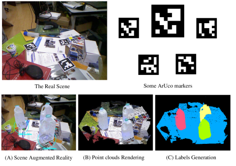
Figure 7: The generation of AR datasets (A) Scene Augmented Reality, (B) Point clouds Rendering, (C) Labels Generation.

As shown in Fig. 7, the method contains three main phases: 1) Scene Augmented Reality, 2) Point clouds Rendering and 3) Labels Generation. Firstly, we set up a scene similar to the testing datasets, and then place specific ArUco markers [37] in it. With this marker system, the method can automatically detecting the markers and get the camera pose transformation of each marker. We use AR technology to visualize the transformed mesh models on the mark boards, and display the accurate 6-DOF changes as the sensor moves. In the process of scene augmented reality, we randomly place the mark boards and judge whether the virtual objects are overlapping through the augmented reality scene. For each class of objects, we capture 2k+ frames under a random view pose. Secondly, based on the principle of light propagation [38] and the parameters of real sensors, we render the virtual objects in augmented reality scene, and the occlusion between objects is also considered in the rendered point clouds data. Finally, since the accurate 6-DOF pose of each object is known, we can easily generate the segmentation, instance label and 3D bounding box of each point in the scene.

In addition to the generated augmented reality scenes, we sample 10% of the testing datasets, remove the targets from the scene and replace them with the rendered point clouds of the object mesh models, which are rotated randomly around the axis perpendicular to the working plane every thirty degrees. For each class of object, we first pre-train the weights of our network on the segmentation task same as [34], and then train our multi-task architecture on the generated augmented reality datasets, final, use the processed sampled testing datasets to fine-tune the weights.

This data enhancement method based on AR technology can be used for data generation of specific scenes quickly, without collecting real scene data and spending a lot of time on manual labeling. However, this method can not be used to generate aliasing scene data for the time being, e.g., the bin-picking, which suffer from the overlapping of the marker boards. This is also the future work we want to solve.

4.2 Results On the the Tejani et al. Dataset [1]

We evaluate the performance of our method on the Tejani et al. dataset [1]. In our experiments, we use the re-annotated dataset by Wadim et al. [10] and compare with five methods. When the distance threshold is less than 15% of the model s diameter, it is claimed that the estimated pose is correct. The statistic recognition results are shown in Table 1, where the overall average F1-Score of our method is the best 87.8%, in comparison with LineMod (74.0%)[2], LC-HF (65.1%)[1], Kehl (74.7%)[10] and Liu (76.8%) [11]. These methods all adopt the traditional similarity search strategy, which need to define the key-point features firstly, and then use the feature search strategy to find the optimal matching features. Compared with these step-by-step methods, our approach is not only a more concise end-to-end strategy, but also shows better results. In addition, method of [2, 1, 10] recognize candidates in 2D images, and finally refines the results using 3D data. Although method of [11] directly uses 3D data, it is transformed into voxel grids for processing, which leads to the reduction of computational efficiency. Our method can process point clouds data directly and predict more accurate 6-DOF pose estimation. Especially for the milk model, since its uniform color surface and symmetric structure, it is a great challenge for methods which only use 2D information to extract features. Due to our method makes full use of 3D spatial information, the local 3D spatial information makes our pipeline more robust.

Table 1: Comparison of our method on the re-annotated version of [10] with LineMod[2], LC-HF[1], Kehl et al. [10], Liu et al. [11] and SSD-6D [13] in terms of f1-score with ADD metric and IOU2D metric.

Objects	[2]	[1]	[10]	[11]	OURS-ADD	[13]	OURS-IOU2D
Coffee	0.942	0.891	0.972	0.977	0.985	0.983	0.987
Shampoo	0.922	0.792	0.910	0.857	0.932	0.892	0.957
Joystick	0.846	0.549	0.892	0.739	0.913	0.997	0.947
Camera	0.589	0.394	0.383	0.681	0.652	0.741	0.716
Juice	0.595	0.883	0.866	0.866	0.874	0.919	0.923
Milk	0.558	0.397	0.463	0.493	0.912	0.780	0.965
Average	0.740	0.651	0.747	0.768	0.878	0.885	0.916

For the results of SSD-6D [13], the F1-Score is calculated when the IoU2D metric of a predicted bounding box with the groundtruth box is higher than 0.5. For a fair comparison, we thus use the IoU2D metric when comparing with SSD-6D [13]. We can see that the average F1-Score is improved relative to ADD metric because of the pose error is partially offset in the projection process. The SSD-6D method that relies on the architecture of SSD method [29] to predict 2D bounding boxes and a very rough orientation of the object in a single step. This is followed by an approximation to estimate the object’s depth from the diagonal length of its 2D bounding box in the image, to lift the 2D detections to 3D. A further pose refinement step is required for improved accuracy, which inevitably increases their running times linearly with the number of objects being detected. Our method is and end-to-end trainable and accurate even without any a posteriori refinement. And since, we do not need further refinement steps.

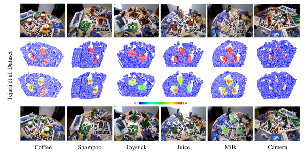
Figure 8: Some demo results on the Tejani et al. dataset [1]. Top-bottom: the recognition results are shown as the 3D bounding box, the results of the point-wise segmentation, the results of the confidence score and the green transformed model overlaid the estimated location. The predicted confidence score are colored by an HSV colormap.

Some results of our method on the Tejani et al. dataset are shown in Fig. 8, where the recognition results are shown as the transformed 3D bounding box. In addition, we also present that the segmentation results and confidence score, we can see that the object points can be accurately segmented and have a higher score.

4.3 Results On the Hinterstoisser et al. Dataset [2]

We evaluate the performance of our method on the Hinterstoisser et al. datasets [2] in terms of Object Recall, where the estimated pose is considered correct when the distance threshold is less than 10% of the models diameter. As shown in Table 2, we compared the two methods and achieved better results. BB8 [14] is a 6-DOF pose estimation pipeline consists of one CNN network to roughly segment the objects and another one to estimate the 2D coordinates projections of the 3D bounding box corners, which are then used to calculate the 6-DOF pose via the PnP algorithm. The multiple step pipeline also requires a further pose refinement for improved accuracy, where the increasing of the number of the objects will directly lead to a linear increase in running times. Compared with BB8, Seamless is a single-shot deep CNN architecture that takes the image as input and directly predicts the 2D projections of the 3D bounding box corners, and then are used to calculate the 6-DOF pose via the PnP algorithm. It is end-to-end trainable and accurate even without any a posteriori refinement. However the networks of Seamless make predictions based on a low-resolution feature map. When global distractions occur, such as occlusions, the feature map is interfered and the pose estimation accuracy drops. By comparison, firstly, our method is an end-to-end pipeline, which can directly predict the 3D bounding box corner coordinates without any PNP like space transformation algorithm, which usually leads to the error of spatial transformation. Secondly, our method can perform point-wise segmentation and box prediction simultaneously, which greatly reduces the impact of global distractions of feature maps. As shown in Table 2, our method has the better results with or without refinement, and use the ICP as the only refinement strategy. The use of 3D point clouds enables our method to make full use of spatial geometric information, which is more reasonable and robust than predicting 3D information in 2D space.

Table 2: Comparison of our method on the Hinterstoisser et al. dataset [2] with BB8 [14], Seamless [15] in terms of add metric with/without refinement.

Methods	without refinement			with refinement
Objects	BB8 [14]	Seamless [15]	OURS	Branchm [12]	BB8 [14]	OURS
ape	27.9	21.62	53.8	33.2	40.4	58.7
bvise	62.0	81.80	76.5	64.8	91.8	83.7
cam	40.1	36.57	55.9	38.4	55.7	62.5
can	48.1	68.80	79.4	62.9	64.1	97.2
cat	45.2	41.82	63.9	42.7	62.6	67.3
driller	58.6	63.51	69.2	61.9	74.4	72.7
duck	32.8	27.23	39.4	30.2	44.3	44.2
eggb	40.0	69.58	63.3	49.9	57.8	70.9
glue	27.0	80.02	74.9	31.2	41.2	81.3
holep	42.4	42.63	50.5	52.8	67.2	75.4
iron	67.0	74.97	61.3	80.0	84.7	67.2
lamp	39.9	71.11	58.2	67.0	76.5	63.3
phone	35.2	47.74	79.7	38.1	54.0	81.2
Average	43.6	55.95	63.5	50.2	62.7	71.2

We also compare the object recall without the refinement using the ADD metric in Table 3 for different thresholds. When the threshold is set as 30%, the accuracy of ours attains the best of 94.12% . In fact, when the threshold is set as 15%, the accuracy of our method exceeded 90%.

Table 3: Comparison of our method on the Hinterstoisser et al. dataset [2] with SSD-6d [13], Seamless [15] using different threshold for add metric without refinement.

Threshold	10%			30%
Methods	[13]	[15]	OURS	[13]	[15]	OURS
Average	2.42	55.95	63.5	31.65	88.25	94.12

Some results of our method on the Hinterstoisser et al. dataset are shown in Fig. 9, where the recognition results are shown as the transformed 3D bounding box. In addition, we also present that the segmentation results and confidence score, we can see that the object points can be accurately segmented and have a higher score.

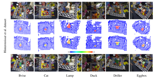
Figure 9: Some demo results on the Hinterstoisser et al. dataset [2]. (top-bottom) the recognition results are shown as the 3D bounding box, the results of the point-wise segmentation, the results of the confidence score and the green transformed model overlaid the estimated location. The predicted confidence score are colored by an HSV colormap.

4.4 Comparison On the Average Running Time

We present the average time comparison of our method with BB8 [14] and Seamless [15] as shown in Tab. 4, where we record the overall speed time and gives the consumption of the refinement process. BB8 takes 140 ms for the segmentation, 130 ms for the pose prediction, and 21 ms for each refinement iteration, which increases the running times linearly with the number of objects being detected. Seamless uses the darknet as the backbone, which achieves high efficiency of 50fps. However, it suffer from the global distractions occur, like occlusions. Our method achieves the recognition speed of 6fps, in which 113ms is used for point clouds sampling&grouping and the remaining is used for prediction. As same as Seamless, ours is also can running without any refinement steps and not affected by the number of objects being detected.

Table 4: compare the average runtime of ours with bb8 [14] and seamless [15].

Methods	Overall Speed	Refinement runtime
BB8 [14]	3 fps	21 ms/object
Seamless [15]	50 fps	without refinement
OURS	6 fps	without refinement

We implement the prediction of the network on the Tensorflow framework with a NVIDIA TITAN XP (12GB RAM), Intel Xeon E3-1226V3 3.3.GHz, 32GB Memory.

5 CONCLUSIONS

In this paper, we propose a simultaneous 3D object segmentation and 6-DOF pose estimation architecture purely in 3D point clouds scenes based on a consensus that one point only belongs to one object, i.e., each point has the potential power to predict the 6-DOF pose of its corresponding object. Ours is concise enough to solve the point-wise 3D object segmentation and 6-DOF pose estimation in 3D point clouds, where others need to convert the irregular point clouds into regular voxel grids or to infer the 3D bounding boxes from 2D images by post-processing of spatial mapping. The various evaluation show that ours can generalize well to multiple scenarios and delivers comparable or surpass performance with the state-of-the-arts. In the future work, we will test the performance of our method on public 3D large-scale datasets with specific training data.

References

- [1] A. Tejani, D. Tang, R. Kouskouridas, T. K. Kim, Latent-class hough forests for 3d object detection and pose estimation, in: ECCV, 2014, pp. 462–477.
- [2] S. Hinterstoisser, V. Lepetit, S. Ilic, S. Holzer, G. Bradski, K. Konolige, N. Navab, Model based training, detection and pose estimation of texture-less 3d objects in heavily cluttered scenes, in: ACCV, 2012, pp. 548–562.
- [3] S. A. A. Shah, M. Bennamoun, F. Boussaid, Keypoints-based surface representation for 3d modeling and 3d object recognition, Pattern Recognition 64 (2017) 29–38.
- [4] C. Cai, N. Somani, A. Knoll, Orthogonal image features for visual servoing of a 6-dof manipulator with uncalibrated stereo cameras, IEEE Transactions on Robotics 32 (2) (2016) 452–461.
- [5] M.-L. Torrente, S. Biasotti, B. Falcidieno, Recognition of feature curves on 3d shapes using an algebraic approach to hough transforms, Pattern Recognition 73 (2018) 111–130.
- [6] H. Liu, F. Sun, B. Fang, D. Guo, Cross-modal zero-shot-learning for tactile object recognition, IEEE Transactions on Systems, Man, and Cybernetics: Systems.
- [7] Y. Cong, G. Sun, J. Liu, H. Yu, J. Luo, User attribute discovery with missing labels, Pattern Recognition 73 (2018) 33–46.
- [8] Y. Guo, F. Sohel, M. Bennamoun, M. Lu, Wan, Rotational projection statistics for 3d local surface description and object recognition, International journal of computer vision 105 (1) (2013) 63–86.
- [9] A. Doumanoglou, R. Kouskouridas, S. Malassiotis, T. K. Kim, Recovering 6d object pose and predicting next-best-view in the crowd, in: CVPR, 2016, pp. 3583–3592.
- [10] W. Kehl, F. Milletari, F. Tombari, S. Ilic, N. Navab, Deep learning of local rgb-d patches for 3d object detection and 6d pose estimation, in: ECCV, 2016, pp. 205–220.
- [11] H. Liu, Y. Cong, S. Wang, H. Fan, D. Tian, Y. Tang, Deep learning of directional truncated signed distance function for robust 3d object recognition, in: IROS, 2017, pp. 5934–5940.
- [12] E. Brachmann, F. Michel, A. Krull, M. Ying Yang, S. Gumhold, et al., Uncertainty-driven 6d pose estimation of objects and scenes from a single rgb image, in: CVPR, 2016, pp. 3364–3372.
- [13] W. Kehl, F. Manhardt, F. Tombari, S. Ilic, N. Navab, Ssd-6d: Making rgb-based 3d detection and 6d pose estimation great again, in: CVPR, 2018.
- [14] M. Rad, V. Lepetit, Bb8: A scalable, accurate, robust to partial occlusion method for predicting the 3d poses of challenging objects without using depth, in: ICCV, Vol. 1, 2017, p. 5.
- [15] B. Tekin, S. N. Sinha, P. Fua, Real-time seamless single shot 6d object pose prediction, in: CVPR, 2018.
- [16] M. Engelcke, D. Rao, D. Z. Wang, C. H. Tong, I. Posner, Vote3deep: Fast object detection in 3d point clouds using efficient convolutional neural networks, in: ICRA, IEEE, 2017, pp. 1355–1361.
- [17] D. Z. Wang, I. Posner, Voting for voting in online point cloud object detection., in: Robotics: Science and Systems, Vol. 1, 2015, pp. 10–15607.
- [18] Y. Zhou, O. Tuzel, Voxelnet: End-to-end learning for point cloud based 3d object detection, in: Proceedings of the IEEE Conference on Computer Vision and Pattern Recognition, 2018, pp. 4490–4499.
- [19] J. M. Morel, G. Yu, Asift: A new framework for fully affine invariant image comparison, SIAM journal on imaging sciences 2 (2) (2009) 438–469.
- [20] D. G. Lowe, Distinctive image features from scale-invariant keypoints, International journal of computer vision 60 (2) (2004) 91–110.
- [21] H. Bay, A. Ess, T. Tuytelaars, L. Van Gool, Speeded-up robust features (surf), Computer vision and image understanding 110 (3) (2008) 346–359.
- [22] A. E. Johnson, M. Hebert, Surface matching for object recognition in complex three-dimensional scenes, Image and Vision Computing 16 (9-10) (1998) 635–651.
- [23] S. M. Yamany, A. A. Farag, Surfacing signatures: An orientation independent free-form surface representation scheme for the purpose of objects registration and matching, IEEE transactions on pattern analysis and machine intelligence 24 (8) (2002) 1105–1120.
- [24] S. Salti, F. Tombari, L. D. Stefano, Shot: Unique signatures of histograms for surface and texture description, Computer vision and image understanding 125 (8) (2014) 251–264.
- [25] Y. Guo, F. Sohel, M. Bennamoun, M. Lu, J. Wan, Trisi: A distinctive local surface descriptor for 3d modeling and object recognition, in: GRAPP/IVAPP, 2015.
- [26] Y. Guo, M. Bennamoun, F. Sohel, M. Lu, J. Wan, N. M. Kwok, A comprehensive performance evaluation of 3d local feature descriptors, International journal of computer vision 116 (1) (2016) 66–89.
- [27] R. Rioscabrera, T. Tuytelaars, Discriminatively trained templates for 3d object detection: A real time scalable approach, in: ICCV, 2014, pp. 2048–2055.
- [28] W. Kehl, F. Tombari, N. Navab, S. Ilic, V. Lepetit, Hashmod: A hashing method for scalable 3d object detection, in: BMVC, 2016.
- [29] W. Liu, D. Anguelov, D. Erhan, C. Szegedy, S. Reed, C.-Y. Fu, A. C. Berg, Ssd: Single shot multibox detector, in: ECCV, Springer, 2016, pp. 21–37.
- [30] V. Lepetit, F. Morenonoguer, P. Fua, Epnp: An accurate o(n) solution to the pnp problem, International Journal of Computer Vision 81 (2) (2009) 155–166.
- [31] J. Redmon, S. Divvala, R. Girshick, A. Farhadi, You only look once: Unified, real-time object detection, in: CVPR, 2016, pp. 779–788.
- [32] D. Chetverikov, D. Svirko, D. Stepanov, P. Krsek, The trimmed iterative closest point algorithm, in: ICPR, Vol. 3, IEEE, 2002, pp. 545–548.
- [33] R. Q. Charles, H. Su, K. Mo, L. J. Guibas, Pointnet: Deep learning on point sets for 3d classification and segmentation, in: CVPR, 2017, pp. 77–85.
- [34] C. R. Qi, L. Yi, H. Su, L. J. Guibas, Pointnet++: Deep hierarchical feature learning on point sets in a metric space, in: NIPS, 2017, pp. 5099–5108.
- [35] C. Moenning, N. A. Dodgson, Fast marching farthest point sampling for implicit surfaces and point clouds, Computer Laboratory Technical Report 565 (2003) 1–12.
- [36] J. S. Vitter, Random sampling with a reservoir, ACM Transactions on Mathematical Software 11 (1) (1985) 37–57.
- [37] S. Garrido-Jurado, R. Muñoz-Salinas, F. J. Madrid-Cuevas, M. J. Marín-Jiménez, Automatic generation and detection of highly reliable fiducial markers under occlusion, Pattern Recognition 47 (6) (2014) 2280–2292.
- [38] R. B. Rusu, S. Cousins, 3d is here: Point cloud library (pcl), in: ICRA, IEEE, 2011, pp. 1–4.