Gluon propagator and three-gluon vertex with dynamical quarks

Abstract

We present a detailed analysis of the kinetic and mass terms associated with the Landau gauge gluon propagator in the presence of dynamical quarks, and a comprehensive dynamical study of certain special kinematic limits of the three-gluon vertex. Our approach capitalizes on results from recent lattice simulations with (2+1) domain wall fermions, a novel nonlinear treatment of the gluon mass equation, and the nonperturbative reconstruction of the longitudinal three-gluon vertex from its fundamental Slavnov-Taylor identities. Particular emphasis is placed on the persistence of the suppression displayed by certain combinations of the vertex form factors at intermediate and low momenta, already known from numerous pure Yang-Mills studies. One of our central findings is that the inclusion of dynamical quarks moderates the intensity of this phenomenon only mildly, leaving the asymptotic low-momentum behavior unaltered, but displaces the characteristic “zero crossing” deeper into the infrared region. In addition, the effect of the three-gluon vertex is explored at the level of the renormalization-group invariant combination corresponding to the effective gauge coupling, whose size is considerably reduced with respect to its counterpart obtained from the ghost-gluon vertex. The main upshot of the above considerations is the further confirmation of the tightly interwoven dynamics between the two- and three-point sectors of QCD.

I Introduction

The three-gluon vertex of QCD Marciano and Pagels (1978); Ball and Chiu (1980); Davydychev et al. (1996); Gracey (2011), to be denoted by $\Gamma_{\alpha\mu\nu}$, has received particular attention in recent years because, in addition to its phenomenological relevance, it displays features that are inextricably connected with subtle dynamical mechanisms operating in the two-point sector of the theory. In particular, the emergence of a gluonic mass scale Cornwall (1982); Bernard (1982, 1983); Donoghue (1984); Wilson et al. (1994); Philipsen (2002); Aguilar et al. (2003), in conjunction with the nonperturbative masslessness of the ghost field Alkofer and von Smekal (2001); Fischer (2006); Aguilar et al. (2008); Boucaud et al. (2008), would appear to account for the “infrared (IR) suppression” of the basic form factors of $\Gamma_{\alpha\mu\nu}$, established in lattice simulations Cucchieri et al. (2006, 2008); Athenodorou et al. (2016); Duarte et al. (2016) as well as in numerous continuum approaches Huber et al. (2012); Pelaez et al. (2013); Aguilar et al. (2014); Blum et al. (2014, 2015); Eichmann et al. (2014); Mitter et al. (2015); Williams et al. (2016); Cyrol et al. (2016); Corell et al. (2018); Aguilar et al. (2019a).

The IR saturation of the Landau gauge gluon propagator Cucchieri and Mendes (2007); Bogolubsky et al. (2007, 2009); Oliveira and Silva (2009); Ayala et al. (2012); Aguilar and Natale (2004); Aguilar and Papavassiliou (2006); Aguilar et al. (2008); Fischer et al. (2009); Boucaud et al. (2008); Dudal et al. (2008); Rodriguez-Quintero (2011); Tissier and Wschebor (2010); Pennington and Wilson (2011); Cloet and Roberts (2014); Fister and Pawlowski (2013); Cyrol et al. (2015); Binosi et al. (2015); Aguilar et al. (2016); Cyrol et al. (2018a), $\Delta(q^{2})$, has been extensively studied within the framework developed from the fusion of the pinch-technique (PT) Cornwall (1982); Cornwall and Papavassiliou (1989); Pilaftsis (1997); Binosi and Papavassiliou (2009) with the background-field method (BFM) Abbott (1981), known as the “PT-BFM scheme” Aguilar and Papavassiliou (2006); Binosi and Papavassiliou (2008). From the dynamical point of view, the saturation is explained by implementing the Schwinger mechanism at the level of the SDE that controls the momentum evolution of $\Delta(q^{2})$ Binosi et al. (2012); Aguilar et al. (2016). In this context, it is natural to regard $\Delta(q^{2})$ as the sum of two distinct components, the “kinetic term”, $J(q^{2})$, and the (momentum-dependent) mass term, $m^{2}(q^{2})$, as shown in Eq. (25). This splitting enforces a special realization of the Slavnov-Taylor identity (STI) satisfied by the fully dressed $\Gamma_{\alpha\mu\nu}$ Binosi et al. (2012), which allows the reconstruction of its longitudinal part by means of a nonperturbative generalization Aguilar et al. (2019a) of the well-known Ball-Chiu (BC) construction Ball and Chiu (1980). Specifically, the 10 longitudinal form factors of $\Gamma_{\alpha\mu\nu}$, to be denoted by $X_{i}$, are fully determined by the $J(q^{2})$, the ghost dressing function, $F(q^{2})$, and three of the five form factors comprising the ghost-gluon kernel, $H_{\mu\nu}$ Ball and Chiu (1980); Davydychev et al. (1996); Aguilar et al. (2019b). However, out of all these ingredients, it is the $J(q^{2})$ that is largely responsible for the main qualitative characteristics of the $X_{i}$ Aguilar et al. (2019a).

As has been explained in earlier works, the SDE governing the $J(q^{2})$ is composed by two types of (dressed) loops, those containing gluons with a dynamically generated mass scale, and those with massless ghosts Aguilar et al. (2014). The former furnish contributions that, due to the presence of the mass, are regulated in the IR, while the latter give rise to “unprotected” logarithms, of the type $\ln(q^{2}/\mu^{2})$, which diverge as $q^{2}\to 0$. The combined effect of these terms is rather striking: as the (Euclidean) momentum $q^{2}$ decreases, $J(q^{2})$ departs gradually from its tree-level value (unity), reverses its sign (“zero crossing”), and finally diverges logarithmically at the origin Aguilar et al. (2014). Quite interestingly, the same overall pattern is displayed by the special combinations of vertex form factors studied in the (quenched) SU(2) lattice simulations of Cucchieri et al. (2006, 2008) and SU(3) Athenodorou et al. (2016); Duarte et al. (2016); Boucaud et al. (2018), exposing the deep connection between the two- and three-point sectors of the theory, encoded in the fundamental STIs.

To date, the three-gluon vertex studies carried out within the PT-BFM framework have been limited to the pure Yang-Mills theory Aguilar et al. (2019a). In the present work, we take a closer look at the structure of this vertex in the presence of dynamical quarks, thus making contact with real-world QCD.

In particular, we present and analyze results for $\Delta(q^{2})$ and $\Gamma_{\alpha\mu\nu}$ obtained from numerical simulations of lattice QCD, using ensembles of gauge fields with $N_{f}=2+1$ domain wall fermions Blum et al. (2016); Boyle et al. (2016, 2017), at the physical point, $m_{\pi}=139$ MeV. These lattice results are complemented by a detailed analysis based on the gluon SDE and the STIs that connect the kinetic term of $\Delta(q^{2})$ with the form factors of $\Gamma_{\alpha\mu\nu}$; for brevity, we will refer to our continuum treatment as “SDE-based”. Within this latter approach, the “unquenched” $J(q^{2})$ is determined following the procedure first introduced in Aguilar et al. (2019c), using as aid the aforementioned lattice results for $\Delta(q^{2})$. Then, the $J(q^{2})$ is employed as the main ingredient of the nonperturbative BC construction introduced in Aguilar et al. (2019a), which provides definite predictions for the two special combinations of vertex form factors, denoted by $\overline{\Gamma}_{1}^{\,\rm sym}(q^{2})$ and $\overline{\Gamma}_{3}^{\,\rm asym}(q^{2})$, considered in our lattice simulation.

The main findings of this work may be summarized as follows. (i) There is excellent agreement between the SDE-based calculation and the lattice data for $\overline{\Gamma}_{1}^{\,\rm sym}(q^{2})$ and $\overline{\Gamma}_{3}^{\,\rm asym}(q^{2})$. (ii) Given that all quark loops are tamed in the IR by the constituent quark masses, the logarithmic divergence displayed by $J(q^{2})$ is still controlled by the ghost-loop, which is essentially insensitive to unquenching effects Ayala et al. (2012). (iii) The deep IR behavior of $\overline{\Gamma}_{1}^{\,\rm sym}(q^{2})$ and $\overline{\Gamma}_{3}^{\,\rm asym}(q^{2})$ is determined by the corresponding asymptotic form of $J(q^{2})$, multiplied by the value of the ghost dressing function at the origin, namely $F(0)$. (iv) The positions of the zero crossings displayed by the unquenched $J(q^{2})$, $\overline{\Gamma}_{1}^{\,\rm sym}(q^{2})$, and $\overline{\Gamma}_{3}^{\,\rm asym}(q^{2})$ move deeper into the IR region with respect to the quenched cases, in agreement with the results reported in Williams et al. (2016). (v) The suppression of $J(q^{2})$, and, correspondingly, of $\overline{\Gamma}_{1}^{\,\rm sym}(q^{2})$ and $\overline{\Gamma}_{3}^{\,\rm asym}(q^{2})$, is about 25% milder than in the quenched case.

The article is organized as follows. In Sec. II we introduce the necessary concepts and notation, and define the quantities studied in the lattice simulation. In Sec. III we present the salient theoretical notions associated with the gluon kinetic term, $J(q^{2})$, and outline the procedure that permits us its indirect determination when dynamical quarks are included. Next, in Sec. IV the SDE-based predictions for $\overline{\Gamma}_{1}^{\,\rm sym}(q^{2})$ and $\overline{\Gamma}_{3}^{\,\rm asym}(q^{2})$ are derived, and subsequently compared with the lattice results. Moreover, the corresponding running couplings are constructed, and directly compared with the corresponding quantity obtained from the ghost-gluon vertex. Finally, in Sec. V we discuss the results and summarize our conclusions.

II The three-gluon vertex: General considerations

In this section we first present the basic definitions and conventions related with the gluon propagator and the three-gluon vertex. Then, we review the two main quantities (vertex projections) that have been evaluated in the lattice simulation reported here.

II.1 Notation and basic properties

Throughout this article we work in the Landau gauge, where the gluon propagator is completely transverse,

$$\Delta^{ab}_{\mu\nu}\left(p\right)\ =\ \langle\widetilde{A}^{a}_{\mu}(p)\widetilde{A}^{b}_{\nu}(-p)\rangle\ =\ \Delta(p^{2})\delta^{ab}P_{\mu\nu}(p)\ ;$$ (1)

$\widetilde{A}_{\mu}^{a}$ are the SU(3) gauge fields in Fourier space, the average $\langle\cdot\rangle$ indicates functional integration over the gauge space, and $P_{\mu\nu}(p)=g_{\mu\nu}-p_{\mu}p_{\nu}/p^{2}$.

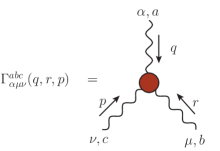
Figure 1: The three-gluon vertex and the corresponding momentum/index conventions.

In addition, we introduce the ghost propagator, $D^{ab}(q^{2})=\delta^{ab}D(q^{2})$, related to its dressing function, $F(q^{2})$, by

$$D(q^{2})=\frac{iF(q^{2})}{q^{2}}\,.$$ (2)

Similarly, in the three-point sector of QCD, one defines the correlation function of three gauge fields, at momenta $q$, $r$, and $p$ (with $q+r+p=0$),

$${\cal G}^{abc}_{\alpha\mu\nu}\left(q,r,p\right)=\ \langle\widetilde{A}_{\mu}^{a}(q)\widetilde{A}_{\nu}^{b}(r)\widetilde{A}_{\rho}^{c}(p)\rangle = f^{abc}{\cal G}_{\alpha\mu\nu}\left(q,r,p\right)\,,$$ (3)

where the connected three-point function ${\cal G}_{\alpha\mu\nu}(q,r,p)$ is given by

$${\cal G}_{\alpha\mu\nu}(q,r,p)=g\,\Gamma_{\alpha^{\prime}\mu^{\prime}\nu^{\prime}}(q,r,p)P^{\alpha^{\prime}}_{\alpha}(q)P^{\mu^{\prime}}_{\mu}(r)P^{\nu^{\prime}}_{\nu}(p)\Delta(q^{2})\Delta(r^{2})\Delta(p^{2})\,,$$ (4)

with $\Gamma_{\alpha\mu\nu}(q,r,p)$ denoting the conventional one-particle irreducible (1-PI) three-gluon vertex (see Fig. 1).

It is customary to introduce the transversally projected vertex, $\overline{\Gamma}_{\alpha\mu\nu}(q,r,p)$, defined as Cucchieri et al. (2006)

$$\overline{\Gamma}_{\alpha\mu\nu}(q,r,p)=\Gamma_{\alpha^{\prime}\mu^{\prime}\nu^{\prime}}(q,r,p)P^{\alpha^{\prime}}_{\alpha}(q)P^{\mu^{\prime}}_{\mu}(r)P^{\nu^{\prime}}_{\nu}(p)\,,$$ (5)

such that

$${\cal G}_{\alpha\mu\nu}(q,r,p)=g\,\overline{\Gamma}_{\alpha\mu\nu}(q,r,p)\Delta(q^{2})\Delta(r^{2})\Delta(p^{2})\,.$$ (6)

Evidently,

$$q^{\alpha}\overline{\Gamma}_{\alpha\mu\nu}(q,r,p)=r^{\mu}\overline{\Gamma}_{\alpha\mu\nu}(q,r,p)=p^{\nu}\overline{\Gamma}_{\alpha\mu\nu}(q,r,p)=0\,.$$ (7)

The vertex $\Gamma_{\alpha\mu\nu}(q,r,p)$ is usually decomposed into two distinct pieces, according to Ball and Chiu (1980); Davydychev et al. (1996); Aguilar et al. (2019c),

$$\Gamma^{\alpha\mu\nu}(q,r,p)=\Gamma_{\!{\scriptscriptstyle L}}^{\alpha\mu\nu}(q,r,p)+\Gamma_{\!{\scriptscriptstyle T}}^{\alpha\mu\nu}(q,r,p)\,,$$ (8)

where the “longitudinal” part, $\Gamma_{\!{\scriptscriptstyle L}}^{\alpha\mu\nu}(q,r,p)$, saturates the corresponding STIs [see Eq. (29)], while the totally “transverse” part, $\Gamma_{\!{\scriptscriptstyle T}}^{\alpha\mu\nu}(q,r,p)$, satisfies Eq. (7).

The tensorial decomposition of $\Gamma_{\!{\scriptscriptstyle L}}^{\alpha\mu\nu}(q,r,p)$ and $\Gamma_{\!{\scriptscriptstyle T}}^{\alpha\mu\nu}(q,r,p)$ reads

$$\Gamma_{\!{\scriptscriptstyle L}}^{\alpha\mu\nu}(q,r,p)=\sum_{i=1}^{10}X_{i}(q,r,p)\ell_{i}^{\alpha\mu\nu}\,,\qquad\Gamma_{\!{\scriptscriptstyle T}}^{\alpha\mu\nu}(q,r,p)=\sum_{i=1}^{4}Y_{i}(q,r,p)t_{i}^{\alpha\mu\nu}\,,$$ (9)

where the explicit expressions of the basis elements $\ell_{i}^{\alpha\mu\nu}$ and $t_{i}^{\alpha\mu\nu}$ are given in Eqs. (3.4) and (3.6) of Aguilar et al. (2019a), respectively.

It is clear that, due to Eq. (7), $\overline{\Gamma}_{\alpha\mu\nu}(q,r,p)$ may be expressed entirely in terms of the 4 tensors $t_{i}^{\alpha\mu\nu}$, i.e.,

$$\overline{\Gamma}^{\alpha\mu\nu}(q,r,p)=\sum_{i=1}^{4}\,\left[Y_{i}(q,r,p)+\sum_{j=1}^{10}c_{ij}\ X_{j}(q,r,p)\right]\,t_{i}^{\alpha\mu\nu}\,.$$ (10)

The presence of the $X_{j}(q,r,p)$ in the final answer may be understood by simply noticing that, after their transverse projection, the elements $\overline{\ell}_{i}^{\alpha\mu\nu}:=\ell_{i}^{\alpha^{\prime}\mu^{\prime}\nu^{\prime}}P_{\alpha^{\prime}}^{\alpha}(q)P_{\mu^{\prime}}^{\mu}(r)P_{\nu^{\prime}}^{\nu}(p)$, can be expressed as linear combinations of the $t_{i}^{\alpha\mu\nu}$; the exact expressions for the $c_{ij}$ may be straightforwardly worked out.

In addition, we define the tree-level analogue of Eq. (5),

$$\overline{\Gamma}_{\!0}^{\alpha\mu\nu}(q,r,p)=\Gamma_{\!0}^{\alpha^{\prime}\mu^{\prime}\nu^{\prime}}(q,r,p)P_{\alpha^{\prime}}^{\alpha}(q)P_{\mu^{\prime}}^{\mu}(r)P_{\nu^{\prime}}^{\nu}(p)\,,$$ (11)

where

$$\Gamma_{\!0}^{\alpha\mu\nu}(q,r,p)=(q-r)^{\nu}g^{\alpha\mu}+(r-p)^{\alpha}g^{\mu\nu}+(p-q)^{\mu}g^{\alpha\nu}\,.$$ (12)

Note finally that, in the Euclidean space, the form factors $X_{i}(q,r,p)$ and $Y_{i}(q,r,p)$ are usually expressed as functions of $q^{2}$, $r^{2}$, and the angle $\theta$ formed between $q$ and $r$, namely $X_{i}(q,r,p)\to X_{i}(q^{2},r^{2},\theta)$ Aguilar et al. (2019a).

II.2 The lattice observables

The lattice two- and three-point correlation functions employed in the present work have been obtained from $N_{f}$=2+1 ensembles published in Blum et al. (2016); Boyle et al. (2016, 2017); they were generated with the Iwasaki action for the gauge sector Iwasaki (1985), and the Domain Wall action for the fermion sector Kaplan (1992); Shamir (1993) (for related reviews, see, e.g.,  Vranas (2001); Kaplan (2009)). In order to reach the physical point, $m_{\pi}=139$ MeV, the Möbius kernel Brower et al. (2005) has been used, resulting in a simulation of light quarks with a mass ranging from 1.3 to 1.6 MeV, while the strange quark mass is 63 MeV; additional information on the particular setups is provided in Table 1. Note that the data for the gluon propagator have been recently presented in Cui et al. (2019), constituting a central ingredient in the construction of the process-independent QCD effective charge. In addition, in an earlier work Zafeiropoulos et al. (2019), the same data were employed in the determination of the strong running coupling at the $Z^{0}$-boson mass within the so-called Taylor scheme. Finally, details on the Landau gauge computation of the gauge fields, and the correlation functions defined in Eqs. (1) and (3), may be found in Ayala et al. (2012); Boucaud et al. (2017). In addition, the treatment of the $O(4)$-breaking artifacts has been carried out as described in Becirevic et al. (1999, 2000); de Soto and Roiesnel (2007); Boucaud et al. (2018).

$\beta$	size	$m_{\pi}$ [MeV]	$a^{-1}$ [GeV]	V [fm4]	confs
2.37	$32^{3}\times 64$	370	3.148	$2.00^{3}\times 4.00$	590
2.25	$64^{3}\times 128$	139.15	2.359	$5.35^{3}\times 10.70$	330
2.13	$48^{3}\times 96$	139.35	1.730	$5.47^{3}\times 10.93$	350
1.63	$48^{3}\times 64$	137.5	0.997	$9.43^{3}\times 12.57$	276

Table 1: Setup parameters for the four lattice ensembles used in this work.

Let us now consider the special quantity

$$T(q,r,p)=\frac{W^{\alpha\mu\nu}(q,r,p){\cal G}_{\alpha\mu\nu}(q,r,p)}{W^{\alpha\mu\nu}(q,r,p)W_{\alpha\mu\nu}(q,r,p)}\,,$$ (13)

where the explicit form of the tensors $W_{\alpha\mu\nu}(q,r,p)$ will be judiciously chosen in order to project out particular components of the connected three-point function, ${\cal G}_{\alpha\mu\nu}(q,r,p)$, in certain simplified kinematic limits. Note that, in general, the quantity $T(q,r,p)$ is comprised of both longitudinal and transverse components, $X_{i}$ and $Y_{i}$.

As in Athenodorou et al. (2016), we focus on two special kinematic configurations:

(i) The totally symmetric limit, obtained when

$$q^{2}=p^{2}=r^{2}:=s^{2}\,,\quad q\cdot p=q\cdot r=p\cdot r=-\frac{s^{2}}{2}\,,\quad\theta=2\pi/3\,.$$ (14)

(ii) The asymmetric limit, corresponding to the kinematic choice

$$p\to 0\,,\quad r=-q\,,\quad\theta=\pi\,.$$ (15)

Starting with case (i), it is relatively straightforward to establish that the application of the symmetric limit in Eq. (14) reduces the tensorial structure of $\overline{\Gamma}^{\alpha\mu\nu}(q,r,p)$ down to Athenodorou et al. (2016)

$$\overline{\Gamma}_{\rm sym}^{\alpha\mu\nu}(q,r,p)=\overline{\Gamma}^{\,\rm sym}_{1}(s^{2})\lambda_{1}^{\alpha\mu\nu}(q,r,p)+\overline{\Gamma}_{2}^{\,\rm sym}(s^{2})\lambda_{2}^{\alpha\mu\nu}(q,r,p)\,,$$ (16)

with

$$\lambda_{1}^{\alpha\mu\nu}(q,r,p)=\overline{\Gamma}_{\!0}^{\alpha\mu\nu}(q,r,p)\ ,\qquad\lambda_{2}^{\alpha\mu\nu}(q,r,p)=\frac{(r-p)^{\alpha}(p-q)^{\mu}(q-r)^{\nu}}{s^{2}}\,.$$ (17)

The form factor $\overline{\Gamma}_{1}^{\,\rm sym}(s^{2})$ is particularly interesting, because it captures certain exceptional features linked to a vast array of underlying theoretical ideas. $\overline{\Gamma}_{1}^{\,\rm sym}(s^{2})$ may be projected out by contracting Eq. (16) with the tensor

$${\widetilde{\lambda}}_{1}^{\alpha\mu\nu}=\lambda_{1}^{\alpha\mu\nu}(q,r,p)+\frac{1}{2}\lambda_{2}^{\alpha\mu\nu}(q,r,p)\,,$$ (18)

which is orthogonal to $\lambda_{2}^{\alpha\mu\nu}(q,r,p)$. Therefore, the substitution $W^{\alpha\mu\nu}(q,r,p)\to{\widetilde{\lambda}}_{1}^{\alpha\mu\nu}(q,r,p)$ at the level of Eq. (13), and the subsequent implementation of Eq. (14) in the resulting expressions, leads to

$$T^{\rm sym}(s^{2}):=T(q,r,p)\,\big{|}_{{\rm Eq.(\ref{defsym})}}^{W\to{\widetilde{\lambda}}_{1}}=g\,\overline{\Gamma}_{1}^{\,\rm sym}(s^{2})\Delta^{3}(s^{2})\,.$$ (19)

As has been shown in Aguilar et al. (2019a), the use of the basis of Eq. (9) allows one to express $\overline{\Gamma}_{1}^{\,\rm sym}(s^{2})$ in the form

$$\overline{\Gamma}_{1}^{\,\rm sym}(s^{2})=X_{1}(s^{2})-\frac{s^{2}}{2}X_{3}(s^{2})+\frac{s^{4}}{4}Y_{1}(s^{2})-\frac{s^{2}}{2}Y_{4}(s^{2})\,.$$ (20)

Turning to case (ii), the implementation of the asymmetric limit gives rise to an expression for $\overline{\Gamma}^{\alpha\mu\nu}(q,r,p)$ given by a single tensor, namely Athenodorou et al. (2016)

$$\overline{\Gamma}_{\rm asym}^{\alpha\mu\nu}(q,r,p)=\overline{\Gamma}_{3}^{\,\rm asym}(q^{2})\lambda_{1}^{\alpha\mu\nu}(q,-q,0)\,,$$ (21)

with

$$\lambda_{1}^{\alpha\mu\nu}(q,-q,0)=2q^{\nu}P^{\alpha\mu}(q)\,.$$ (22)

Setting $W\to\lambda_{1}^{\alpha\mu\nu}(q,-q,0)$ into Eq. (13), one obtains

$$T^{\rm asym}(q^{2}):=T(q,r,p)\,\big{|}_{{\rm Eq.(\ref{defasym})}}^{W\to\lambda_{1}}=g\overline{\Gamma}_{3}^{\,\rm asym}(q^{2})\Delta(0)\Delta^{2}(q^{2})\,.$$ (23)

Again, using Eq. (9), we may cast $\overline{\Gamma}_{3}^{\,\rm asym}(q^{2})$ in the form Aguilar et al. (2019a)

$$\overline{\Gamma}_{3}^{\,\rm asym}(q^{2})=X_{1}(q^{2},q^{2},\pi)-q^{2}X_{3}(q^{2},q^{2},\pi)\,.$$ (24)

Interestingly, $\overline{\Gamma}_{3}^{\,\rm asym}(q^{2})$ does not contain any reference to the transverse form factors $Y_{i}$, and may be therefore determined in its entirety by the nonperturbative BC construction of Aguilar et al. (2019a).

III The kinetic term of the gluon propagator

In this section we take a closer look at the kinetic term of the gluon propagator, which, by virtue of the fundamental STIs, is closely connected with the longitudinal form factors $X_{i}$, introduced in Eq. (9). After reviewing certain salient theoretical concepts related to this quantity, we outline its indirect derivation from the unquenched gluon propagator and the corresponding gluon mass equation, and discuss some of its most outstanding properties.

III.1 Basic concepts and key relations

A special feature of $\Delta(q^{2})$, observed in the Landau gauge, is its saturation in the deep IR Cornwall (1982); Aguilar et al. (2008, 2017). This property has been firmly established in a variety of SU(2) Cucchieri and Mendes (2007, 2008, 2010) and SU(3) Bogolubsky et al. (2007); Boucaud et al. (2006); Bowman et al. (2007); Bogolubsky et al. (2009); Oliveira and Silva (2009); Ayala et al. (2012); Bicudo et al. (2015) large-volume lattice simulations, both quenched and unquenched. Due to its far reaching theoretical implication, this property has been scrutinized in the continuum using a multitude of distinct approaches Aguilar and Natale (2004); Aguilar and Papavassiliou (2006); Braun et al. (2010); Epple et al. (2008); Aguilar et al. (2008); Fischer et al. (2009); Boucaud et al. (2008); Dudal et al. (2008); Rodriguez-Quintero (2011); Tissier and Wschebor (2010); Pennington and Wilson (2011); Cloet and Roberts (2014); Serreau and Tissier (2012); Aguilar et al. (2016); Fister and Pawlowski (2013); Binosi et al. (2015); Cyrol et al. (2015, 2018a).

This characteristic behavior of $\Delta(q^{2})$ is considered to be intimately connected with the emergence of a gluon mass scale Cornwall (1982); Philipsen (2002); Aguilar et al. (2003), and has been studied in detail within the framework of the “PT-BFM” Aguilar and Papavassiliou (2006); Binosi and Papavassiliou (2008). For the purposes of the present work, we will briefly comment on a limited number of concepts and ingredients related with this particular approach; for further details, the reader is referred to the extended literature cited above.

(a) The IR finiteness of $\Delta(q^{2})$ motivates the splitting of its inverse into two separate components, according to (Euclidean space) Binosi et al. (2012)

$$\Delta^{-1}(q^{2})=q^{2}J(q^{2})+m^{2}(q^{2})\,,$$ (25)

where $J(q^{2})$ corresponds to the so-called “kinetic term” [at tree-level, $J(q^{2})=1$], while $m^{2}(q^{2})$ to a momentum-dependent gluon mass scale, with the property $m^{2}(0)=\Delta^{-1}(0)$. Note that we have suppressed the dependence of all quantities appearing in Eq. (25) on the renormalization point $\mu$. For large values of $q^{2}$, the component $J(q^{2})$ captures the standard perturbative corrections to the gluon propagator, while in the IR it exhibits exceptional nonperturbative features Aguilar et al. (2014, 2019a).

(b) The emergence of the component $m^{2}(q^{2})$ is triggered by the non-Abelian realization of the well-known Schwinger mechanism Schwinger (1962a, b) for gauge boson mass generation. This latter mechanism is activated through the inclusion of longitudinally coupled massless poles into the three-gluon vertex that enters in the SDE governing the evolution of $\Delta^{-1}(q^{2})$ Aguilar et al. (2012a); Binosi et al. (2012); Ibañez and Papavassiliou (2013); Binosi and Papavassiliou (2018); Aguilar et al. (2018). In particular, one implements the replacement

$$\Gamma_{\alpha\mu\nu}\to{\rm{I}}\!\Gamma_{\alpha\mu\nu}=\Gamma_{\alpha\mu\nu}+V_{\alpha\mu\nu}\,,$$ (26)

where $V_{\alpha\mu\nu}$ contains the aforementioned poles, arranged in the special tensorial structure Ibañez and Papavassiliou (2013)

$$V_{\alpha\mu\nu}(q,r,p)=\left(\frac{q_{\alpha}}{q^{2}}\right)A_{\mu\nu}(q,r,p)+\left(\frac{r_{\mu}}{r^{2}}\right)B_{\alpha\nu}(q,r,p)+\left(\frac{p_{\nu}}{p^{2}}\right)C_{\alpha\mu}(q,r,p)\,.$$ (27)

Consequently, by virtue of the relation $V_{\alpha^{\prime}\mu^{\prime}\nu^{\prime}}(q,r,p)P^{\alpha^{\prime}}_{\alpha}(q)P^{\mu^{\prime}}_{\mu}(r)P^{\nu^{\prime}}_{\nu}(p)=0$, the component $V_{\alpha\mu\nu}(q,r,p)$ drops out from the quantity $T(q,r,p)$ defined in Eq. (13), and only the “no-pole” part of the vertex, $\Gamma_{\alpha\mu\nu}$, contributes to it.

(c) It turns out that the two functions composing $\Delta^{-1}(q^{2})$ in Eq. (25) and the two vertices comprising ${\rm{I}}\!\Gamma_{\alpha\mu\nu}$ in Eq. (26) are firmly linked. Specifically, the STI satisfied by ${\rm{I}}\!\Gamma_{\alpha\mu\nu}(q,r,p)$,

$$q^{\alpha}{\rm{I}}\!\Gamma_{\alpha\mu\nu}(q,r,p)=F(q^{2})[\Delta^{-1}(p^{2})P^{\alpha}_{\nu}(p)H_{\alpha\mu}(p,q,r)-\Delta^{-1}(r^{2})P^{\alpha}_{\mu}(r)H_{\alpha\nu}(r,q,p)]\,,$$ (28)

is naturally separated into two “partial” ones, relating the divergences of $\Gamma_{\alpha\mu\nu}$ and $V_{\alpha\mu\nu}$ with $J(q^{2})$ and $m^{2}(q^{2})$, respectively, namely

$$q^{\alpha}\Gamma_{\alpha\mu\nu}(q,r,p) = F(q^{2})[p^{2}J(p^{2})P^{\alpha}_{\nu}(p)H_{\alpha\mu}(p,q,r)-r^{2}J(r^{2})P^{\alpha}_{\mu}(r)H_{\alpha\nu}(r,q,p)]\,,$$ (29)

$$q^{\alpha}V_{\alpha\mu\nu}(q,r,p) = F(q^{2})[m^{2}(r^{2})P^{\alpha}_{\mu}(r)H_{\alpha\nu}(r,q,p)-m^{2}(p^{2})P^{\alpha}_{\nu}(p)H_{\alpha\mu}(p,q,r)]\,.$$ (30)

The practical implication of this separation is that the form factors $X_{i}$ of $\Gamma_{\!{\scriptscriptstyle L}}^{\alpha\mu\nu}(q,r,p)$ may be reconstructed by means of a nonperturbative generalization Aguilar et al. (2019a) of the well-known BC procedure Ball and Chiu (1980). In particular, the $X_{i}$ are expressed as combinations of the $J(q^{2})$, the ghost dressing function, $F(q^{2})$, and three of the five components appearing in the tensorial decomposition of $H_{\mu\nu}$, whose one-loop dressed approximation has been computed in Aguilar et al. (2019b). These results are especially relevant for the study in hand, because they provide a theoretical (albeit approximate) handle on the form of the $X_{i}$ appearing in Eqs. (20) and (24); note, however, that the $Y_{i}$ remain undetermined by this procedure.

(d) The special realization of the STIs explained in point (c) leads to the separation of the original SDE governing $\Delta(q^{2})$ into a system of two coupled integral equations, one determining $J(q^{2})$ and the other $m^{2}(q^{2})$ Binosi et al. (2012). As has been demonstrated recently in Aguilar et al. (2019c), the self-consistent treatment of the equation controlling $m^{2}(q^{2})$, in conjunction with the (quenched) lattice data for $\Delta(q^{2})$, permits one to pin down the form of $J(q^{2})$ quite accurately, without actually invoking its own (considerably more complicated) integral equation. The subsequent use of this $J(q^{2})$ as ingredient in the BC construction of the $X_{i}$ described above, allows one to obtain, through Eqs. (20) and (24), SDE-derived predictions for $T^{\rm sym}(s^{2})$ and $T^{\rm asym}(q^{2})$, which are in excellent agreement with the lattice data of Athenodorou et al. (2016).

III.2 The “unquenched” $J(q^{2})$: general construction and main results

The above considerations, and in particular the procedure summarized in point (d), will be applied in the present work in order to obtain SDE-derived predictions for the unquenched $\overline{\Gamma}^{\,\rm sym}_{1}(s^{2})$ and $\overline{\Gamma}_{3}^{\,\rm asym}(q^{2})$, which will be subsequently compared with the corresponding sets of lattice results. In what follows we outline the main points of this construction, postponing the multitude of technical details for a future communication.

($\rm P_{1}$): The starting point is the gluon mass equation considered in Aguilar et al. (2019c), whose general form is given by ($\alpha_{s}:=g^{2}/4\pi$)

$$m^{2}(q^{2})=\int\frac{\mathrm{d}^{4}k}{(2\pi)^{4}}\,m^{2}(k)\Delta(k)\Delta(k+q){\cal K}(k,q,\alpha_{s}),$$ (31)

where the kernel ${\cal K}$ receives one-loop and two-loop dressed contributions.

($\rm P_{2}$): The effective treatment of multiplicative renormalization amounts to the substitution of the vertex renormalization constants, multiplying the one- and two-loop components of ${\cal K}$, by kinematically simplified form factors of the three- and four-gluon vertices, denoted by ${\cal C}_{3}(k^{2})$ and ${\cal C}_{4}(k^{2})$, respectively.

($\rm P_{3}$): The kinetic term $J(q^{2})$ enters into the gluon mass equation when the substitution given in Eq. (25) is implemented at the level of the term $\Delta(k)\Delta(k+q)$. In addition, the function ${\cal C}_{3}(k^{2})$ depends on $J(k^{2})$; specifically, for its derivation we adopt the Abelian version of the BC construction Ball and Chiu (1980), setting the ghost dressing function and the ghost-gluon kernel at their tree-level values, which yields simply ${\cal C}_{3}(k^{2})=J(k^{2})$.

($\rm P_{4}$): The term ${\cal C}_{4}(k^{2})$ is approximated by the same functional form given in Eq. (4.8) of Aguilar et al. (2019c). As explained there, the main feature of ${\cal C}_{4}(k^{2})$, which is instrumental for the stability of the gluon mass equation, is its mild enhancement with respect to its tree-level value in the critical region of a few hundred MeV.

($\rm P_{5}$): An initial Ansatz for $J(q^{2})$ is introduced as a “seed”, and is subsequently improved by means of a well-defined iterative procedure, described in detail in Sec. VB of Aguilar et al. (2019c). In particular, both the form of $J(q^{2})$ and the value of $\alpha_{s}$ are gradually modified, and each time the corresponding solution, $m^{2}(q^{2})$, obtained from the gluon mass equations, is recorded. The procedure terminates when the pair $\{m^{2}(q^{2}),J(q^{2})\}$ has been identified which, when combined according to Eq. (25), provides the best possible coincidence with the lattice data for $\Delta(q^{2})$ with $N_{f}=2+1$ [see the left bottom panel of Fig. 2]. The final value of the gauge charge is $\alpha_{s}=0.27$.

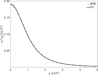
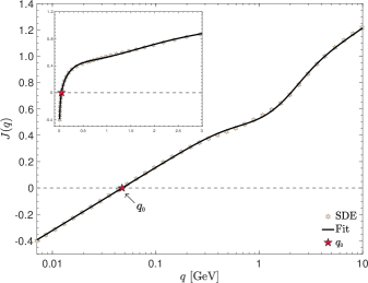
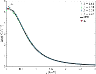
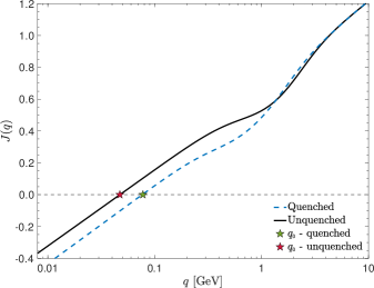
Figure 2: Top left panel: The dynamical gluon mass, $m^{2}(q)$, obtained from Eq. (31) and fitted by Eq. (32). Top right panel: The $J(q)$ obtained through the procedure described in points ($P_{1}$)-($P_{5}$), and the corresponding fit, given in Eq. (33). Bottom left panel: Comparison of the unquenched gluon propagator, $\Delta(q)$, obtained from Eq. (25) (black continuous), with the lattice data (solid circles in different colors for each $\beta$). Bottom right panel: The quenched (blue dashed) and unquenched (black continuous) $J(q)$; the stars indicate the momentum $q_{\scriptscriptstyle\mathrm{0}}$ where $J(q_{\scriptscriptstyle\mathrm{0}})=0$.

An excellent fit for $m^{2}(q^{2})$, shown in the top left panel of Fig. 2, is given by

$$m^{2}(q^{2})=\frac{m_{\scriptscriptstyle\mathrm{0}}^{4}}{\kappa_{\scriptscriptstyle\mathrm{1}}^{2}+q^{2}\ln[(q^{2}+\kappa_{\scriptscriptstyle\mathrm{2}}^{2})/\sigma^{2}]}\,,$$ (32)

where the parameters are given by $m_{\scriptscriptstyle\mathrm{0}}^{4}=0.134$ GeV⁴, $\kappa_{\scriptscriptstyle\mathrm{1}}^{2}=0.705$ GeV², $\kappa_{\scriptscriptstyle\mathrm{2}}^{2}=9.31$ GeV², and $\sigma^{2}=5.13$ GeV².

Similarly, the solution for $J(q^{2})$, shown in the top right panel of Fig. 2, is accurately fitted by

$$J(q^{2})=1+\frac{3\lambda_{s}}{4\pi}\left(1+\frac{\tau_{\scriptscriptstyle\mathrm{1}}}{q^{2}+\tau_{\scriptscriptstyle\mathrm{2}}}\right)\left[2\ln\left(\frac{q^{2}+\eta^{2}(q^{2})}{\mu^{2}+\eta^{2}(\mu^{2})}\right)+\frac{1}{6}\ln\left(\frac{q^{2}}{\mu^{2}}\right)\right]\,,$$ (33)

with

$$\eta^{2}(q^{2})=\frac{\eta_{\scriptscriptstyle\mathrm{1}}}{q^{2}+\eta_{\scriptscriptstyle\mathrm{2}}}\,,$$ (34)

where $\lambda_{s}=0.237$, $\tau_{\scriptscriptstyle\mathrm{1}}=7.06$ GeV², $\tau_{\scriptscriptstyle\mathrm{2}}=0.709$ GeV², $\eta_{\scriptscriptstyle\mathrm{1}}=22.35$ GeV⁴, $\eta_{\scriptscriptstyle\mathrm{2}}=1.19$ GeV², and $\mu^{2}=18.64$ GeV². Notice that $J(\mu^{2})=1$, as required by the momentum subtraction (MOM) renormalization prescription.

We emphasize that, even though several aspects of the unquenched gluon propagator have been previously addressed within the PT-BFM formalism Aguilar et al. (2012b, 2013a), the results presented in Eqs. (32) and (33) are completely new.

III.3 Asymptotic analysis for the deep IR

By expanding the above fits for $J(q^{2})$ and $m^{2}(q^{2})$ around $q^{2}\to 0$, we obtain

$$J(q^{2})=a\ln\left(\frac{q^{2}}{\mu^{2}}\right)+b\,,\qquad m^{2}(q^{2})=d+c\,q^{2}\,,$$ (35)

and therefore

$$\Delta^{-1}(q^{2})=d+q^{2}\left[a\ln\left(\frac{q^{2}}{\mu^{2}}\right)+b+c\right]\,,$$ (36)

with

$$\displaystyle a= \displaystyle\frac{\lambda_{s}}{8\pi}\left(1+\frac{\tau_{\scriptscriptstyle\mathrm{1}}}{\tau_{\scriptscriptstyle\mathrm{2}}}\right)\,,\qquad b= \displaystyle 1+\frac{3\lambda_{s}}{2\pi}\left(1+\frac{\tau_{\scriptscriptstyle\mathrm{1}}}{\tau_{\scriptscriptstyle\mathrm{2}}}\right)\ln\left[\frac{\eta_{\scriptscriptstyle\mathrm{1}}}{\eta_{\scriptscriptstyle\mathrm{2}}\left[\mu^{2}+\eta^{2}(\mu^{2})\right]}\right]\,,$$

$$\displaystyle c= \displaystyle-\frac{m_{\scriptscriptstyle\mathrm{0}}^{4}}{\kappa_{\scriptscriptstyle\mathrm{1}}^{4}}\ln\left(\frac{\kappa_{\scriptscriptstyle\mathrm{2}}^{2}}{\sigma^{2}}\right)\,,\qquad d= \displaystyle\frac{m_{\scriptscriptstyle\mathrm{0}}^{4}}{\kappa_{\scriptscriptstyle\mathrm{1}}^{2}}\,.$$ (37)

Employing the numerical values of the parameters in Eqs.(33) and (34), one obtains $a=0.104$, $b=0.934$, $c=-0.160$, $d=0.190$ GeV².

With the above asymptotic expressions at our disposal, we proceed to elaborate on the following important points.

(i) As can be seen in the bottom right panel of Fig. 2, for momenta lower than about $500$ MeV, the quenched and unquenched $J(q^{2})$ run nearly parallel to each other. In view of Eq. (35), this indicates that the coefficient of the logarithm remains practically unchanged in the presence of quark loops, whose net effect in the deep IR is to simply modify (increase) the numerical value of the constant $b$, thus shifting the position of the zero crossing towards lower momenta. A qualitative explanation of these observations may be given by noting that (a) the ghost dressing function is rather insensitive to unquenching effects Ayala et al. (2012), and hence, the contribution of the ghost loops is essentially the same, and (b) the quark loops provide IR finite contributions, since the corresponding logarithms are protected by the quark masses; their size and sign is consistent with the analysis presented in Aguilar et al. (2012b). It is important to emphasize, however, that throughout our present derivation, no quark loops have been actually evaluated; instead, by means of the optimization procedure described in ($\rm P_{5}$), the effects of the dynamical quarks, implicit in the lattice data for $\Delta(q^{2})$, have been indirectly transmitted to the individual components $J(q^{2})$ and $m^{2}(q^{2})$.

(ii) From Eq. (35) we can obtain a particularly accurate estimate of the position of the “zero crossing”, i.e., the momentum $q_{\scriptscriptstyle\mathrm{0}}$ for which $J(q_{\scriptscriptstyle\mathrm{0}})=0$; it is given by

$$q_{\scriptscriptstyle\mathrm{0}}=\mu\,e^{-\frac{b}{2a}}\,.$$ (38)

With the values of the coefficients found before, this leads to $q_{\scriptscriptstyle\mathrm{0}}=48.19$ MeV. On the other hand, computing the crossing of the full fit of Eq. (33) numerically yields $q_{\scriptscriptstyle\mathrm{0}}=47.18$ MeV [see the red star in the bottom right panel of Fig. 2]. Thus, the asymptotic form is accurate to within $0.3\%$ for the position of the crossing of $J(q^{2})$.

(iii) Let us next consider the maximum of $\Delta(q^{2})$, and denote by $q_{*}$ the momentum where it occurs, namely the solution of the condition $\Delta^{\prime}(q^{2})=0$, where the “prime” denotes differentiation with respect to $q^{2}$. The appearance of this maximum is inextricably connected with the presence of the unprotected logarithm originating from the ghost loop. In addition to confirming the known nonperturbative behavior of the ghost propagator in Euclidean space (i.e., absence of a “ghost mass”), it has a direct implication on the general analytic structure of the gluon propagator Cyrol et al. (2018a); Kern et al. (2019). In particular, from the standard Källén-Lehmann representation Kallen (1952); Lehmann (1954)

$$\Delta(q^{2})=\int_{0}^{\infty}\!\!dt\,\frac{\rho(t)}{q^{2}+t}\,,$$ (39)

where $\rho\,(t)$ is the gluon spectral function, we have that

$$\Delta^{\prime}(q^{2})=-\int_{0}^{\infty}\!\!dt\,\frac{\rho(t)}{(q^{2}+t)^{2}}\,.$$ (40)

Then, the maximum for $\Delta(q^{2})$ at $q^{2}=q^{2}_{*}$ leads necessarily to positivity violation Osterwalder and Schrader (1973, 1975); Alkofer and von Smekal (2001); Cornwall (2013), because the condition

$$\int_{0}^{\infty}\!\!dt\,\frac{\rho(t)}{(q^{2}_{*}+t)^{2}}=0\,,$$ (41)

may be fulfilled only if $\rho(t)$ is not positive-definite.

A reasonable estimate for the value of $q_{*}$ may be derived from Eq. (36); specifically one obtains the equation

$$[\Delta^{-1}(q^{2})]^{\prime}=a\ln\left(\frac{q^{2}}{\mu^{2}}\right)+{\tilde{c}}=0\,,$$ (42)

where ${\tilde{c}}:=a+b+c$, whose solution is given by

$$q_{*}=\mu\exp\left(-\frac{{\tilde{c}}}{2a}\right)\,,$$ (43)

yielding the numerical value $q_{*}=63$ MeV.

The expression for the gluon propagator at the maximum is given by

$$\Delta_{*}:=\Delta(q^{2}_{*})=\left[d-a\mu^{2}\exp\left(-\frac{{\tilde{c}}}{a}\right)\right]^{-1}\,,$$ (44)

its numerical value is given by $\Delta_{*}=5.28$ GeV^-2.

(iv) Finally, we turn to another characteristic feature associated with the presence of the unprotected logarithm, namely the logarithmic divergence of $\Delta^{\prime}(q^{2})$ at the origin. In particular, using Eq. (36), it is straightforward to establish that

$$\Delta^{\prime}(q^{2})\mbox{\raisebox{-5.16663pt}[0.0pt][6.88889pt]{$\stackrel{{\scriptstyle\simeq}}{{\scriptscriptstyle q^{2}\to 0}}$}}-\frac{a}{d^{2}}\ln\left(\frac{q^{2}}{\mu^{2}}\right)\to+\infty\,,\qquad[\Delta^{-1}(q^{2})]^{\prime}\mbox{\raisebox{-5.16663pt}[0.0pt][6.88889pt]{$\stackrel{{\scriptstyle\simeq}}{{\scriptscriptstyle q^{2}\to 0}}$}}a\ln\left(\frac{q^{2}}{\mu^{2}}\right)\to-\infty\,.$$ (45)

(v) While the functional form of $\Delta^{-1}(q^{2})$ is motivated by sound theoretical considerations, the numerical values for the parameters $a$, $b$, $c$, and $d$, quoted below Eq. (37), have been obtained by fitting the entire range of the SDE solution. It would be therefore interesting to probe the stability of our asymptotic results by contrasting them directly with the low-momentum domain of the lattice data, and subsequently refitting the aforementioned parameters. To that end, we consider only the lattice ensemble with $\beta$=1.63, because it contains the largest number of points in the desired region. Our fitting procedure is limited to the data below a given momentum cutoff, $q_{\scriptscriptstyle\mathrm{cut}}$; we have chosen two values for it, namely $q_{\scriptscriptstyle\mathrm{cut}}$=0.3 GeV and $q_{\scriptscriptstyle\mathrm{cut}}$=0.4 GeV. The result of this analysis can be found in Fig. 3 and in Table 2.

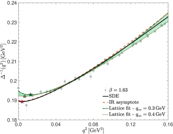
Figure 3: The green band represents the asymptotic fits for the lattice data (gray solid circles) with $q_{{\scriptscriptstyle\mathrm{cut}}}=0.3$ GeV (green dash-dotted line) and $q_{\scriptscriptstyle\mathrm{cut}}=0.4$ GeV (green dashed curve), given by Eq. (36). The black continuous line corresponds to the SDE-based result, while the red dashed curve is its asymptotic limit. All asymptotic curves are given by Eq. (36), with the corresponding fitting parameters listed in the Table 2.

The black continuous line corresponds to the SDE-based result, while the red dashed curve is its asymptotic limit. All asymptotic curves are obtained with Eq. (36) using the fitting parameters listed in the Table 2.

IR asymptotic fits	$a$	$b+c$	$d$ [GeV2]	$q_{*}$ [MeV]
Lattice - ${q_{\scriptscriptstyle\mathrm{cut}}=0.3}$ [GeV]	0.165	1.036	0.195	113
Lattice - ${q_{\scriptscriptstyle\mathrm{cut}}=0.4}$ [GeV]	0.107	0.746	0.193	82
SDE expansion	0.104	0.774	0.190	63

Table 2: Fitting parameters of Eq. (36) for different values of the cutoff $q_{\scriptscriptstyle\mathrm{cut}}$ considered in the fitting process of the lattice data with $\beta=1.63$. In the last line, we show the fitting parameters of the SDE asymptotic limit, given by Eq. (36), which was obtained by expanding the result given in Eqs. (32) and (33). In the last column, we quote the momentum $q_{*}$, where the minimum of $\Delta^{-1}(q^{2})$ [or maximum of $\Delta(q^{2})$] occurs for each case.

As we can see in Fig. 3, the asymptotic expression of Eq. (36) describes the lattice data particularly well. Essentially, the difference between the asymptotic limit of the SDE result (red dashed line) and the best fits for the IR lattice points (green band) appears for very low momenta, and is of the order of $3\%$. The lattice data for $\Delta^{-1}(q^{2})$ show a linear behavior, consistent with a $q^{2}$-increase, except for momenta below 180 MeV, where the effect of the logarithm in Eq. (36) becomes apparent. Note also the onset of a steep derivative close to the origin, in qualitative agreement with point (iv). In addition, the refitted values of $a$, $b+c$, and $d$ are completely consistent with those obtained from the full-range fit of the SDE result.

IV IR suppression of the three-gluon vertex

In this section we present the SDE-based computation of $\overline{\Gamma}^{\,\rm sym}_{1}(s^{2})$ and $\overline{\Gamma}_{3}^{\,\rm asym}(q^{2})$. After an instructive study of the low-momentum limit, our results for the entire range of momenta are presented and compared with the new lattice data. In addition, the two effective couplings obtained from $\overline{\Gamma}^{\,\rm sym}_{1}(s^{2})$ and $\overline{\Gamma}_{3}^{\,\rm asym}(q^{2})$ are constructed, and the former is compared with the corresponding quantity obtained from the ghost-gluon vertex.

IV.1 The SDE-based derivation

The detailed form of the function $J(q^{2})$ captured by Eq. (33) constitutes a key ingredient for the approximate evaluation of the vertex form factors $\overline{\Gamma}^{\,\rm sym}_{1}(s^{2})$ and $\overline{\Gamma}_{3}^{\,\rm asym}(q^{2})$ by means of the main equations Eq. (20) and Eq. (24), respectively. This becomes possible because the nonperturbative BC construction of Aguilar et al. (2019a) allows one to express the $X_{i}$ in terms of the kinetic term of the gluon propagator, the ghost dressing function, and the ghost-gluon form factors. Even though this procedure does not determine the terms $(s^{4}/{4})Y_{1}(s^{2})-({s^{2}}/{2})Y_{4}(s^{2})$ contributing to $\overline{\Gamma}^{\,\rm sym}_{1}(s^{2})$, the overall agreement with the (admittedly error-burdened) lattice results suggests that their omission does not alter drastically the qualitative features of the BC solution; see also the related discussions in Sec. IV.3.

Focusing precisely on $\overline{\Gamma}_{1}^{\,\rm sym}(s^{2})$, the part that depends on the two longitudinal components is given by Aguilar et al. (2019a)

$$X_{1}(s^{2})-\frac{s^{2}}{2}X_{3}(s^{2})=F(s^{2})\left[J(s^{2})\left(H_{1}(s^{2})+\frac{s^{2}}{2}H_{3}(s^{2})\right)+\frac{s^{2}}{2}\,\frac{dJ(s^{2})}{ds^{2}}\,H_{2}(s^{2})\right]\,,$$ (46)

where

$$H_{1}(s^{2}) = A_{1}(s^{2})-\frac{s^{2}}{2}A_{3}(s^{2})\,,$$

$$H_{2}(s^{2}) = A_{1}(s^{2})+\frac{s^{2}}{2}\left[A_{3}(s^{2})-A_{4}(s^{2})\right]\,,$$

$$H_{3}(s^{2}) = A_{1}^{(1,0,0)}(s^{2})+\frac{\sqrt{3}}{2s^{2}}A_{1}^{(0,0,1)}(s^{2})+\frac{s^{2}}{2}\left[A_{3}^{(1,0,0)}(s^{2})-A_{4}^{(1,0,0)}(s^{2})\right]$$ (47)

$$+ \frac{\sqrt{3}}{4}\left[A_{3}^{(0,0,1)}(s^{2})-A_{4}^{(0,0,1)}(s^{2})\right]\,,$$

with the partial derivatives defined as

$$A_{i}^{(1,0,0)}(s^{2})= \left.\frac{\partial A_{i}(q^{2},r^{2},\theta)}{\partial q^{2}}\right|_{q^{2}=r^{2}=s^{2},\,\theta=2\pi/3}\,,$$

$$A_{i}^{(0,1,0)}(s^{2})= \left.\frac{\partial A_{i}(q^{2},r^{2},\theta)}{\partial r^{2}}\right|_{q^{2}=r^{2}=s^{2},\,\theta=2\pi/3}\,,$$

$$A_{i}^{(0,0,1)}(s^{2})= \left.\frac{\partial A_{i}(q^{2},r^{2},\theta)}{\partial\theta}\right|_{q^{2}=r^{2}=s^{2},\,\theta=2\pi/3}\,.$$ (48)

Analogous relations, not reported here, hold for the asymmetric configuration.

Before turning to the full construction of $\overline{\Gamma}^{\,\rm sym}_{1}(s^{2})$, we focus on certain global aspects that it displays at low momenta, which may be obtained from the above expressions with a moderate amount of effort.

IV.2 The low-momentum limit

In particular, Eq. (46) allows one to deduce the exact functional form of $\overline{\Gamma}_{1}^{\,\rm sym}(s^{2})$ in the limit $s^{2}\to 0$. Indeed, a preliminary one-loop dressed analysis reveals that, in that limit, the combination $(s^{4}/4)Y_{1}(s^{2})-(s^{2}/2)Y_{4}(s^{2})$ yields a constant term, to be denoted by $C_{t}$. Moreover, $s^{2}H_{3}(s^{2})$, $s^{2}A_{3}(s^{2})$ and $s^{2}A_{4}(s^{2})$ vanish, while $A_{1}(0)=1$, by virtue of the Taylor theorem Taylor (1971). Consequently, the leading contribution originates from the combination $F(s^{2})[J(s^{2})+(s^{2}/2)J^{\prime}(s^{2})]$.

Then, it is straightforward to establish from Eq. (33) that $\lim\limits_{s^{2}\to 0}s^{2}J^{\prime}(s^{2})=a$. Thus, the asymptotic form of $\overline{\Gamma}_{1}^{\,\rm sym}(s^{2})$ is given by

$$\overline{\Gamma}_{1}^{\,\rm sym}(s^{2})\mbox{\raisebox{-5.16663pt}[0.0pt][6.88889pt]{$\stackrel{{\scriptstyle\simeq}}{{\scriptscriptstyle s^{2}\to 0}}$}}F(0)\left[a\ln\left(\frac{s^{2}}{\mu^{2}}\right)+b+\frac{a}{2}\right]={\tilde{a}}\ln\left(\frac{s^{2}}{\mu^{2}}\right)+{\tilde{b}}\,,$$ (49)

where we have set $C_{t}=0$. Then, using the fact that the saturation value of the ghost dressing function is $F(0)=2.92$ when one renormalizes at $\mu=4.3$ GeV, together with the values for $a$ and $b$ quoted below Eq. (37), one finds ${\tilde{a}}=0.303$ and ${\tilde{b}}=2.87$.

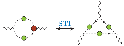
Figure 4: The ghost loop diagram contributing to the kinetic term $J(q^{2})$, and the ghost triangle diagram entering in the skeleton expansion of three-gluon vertex. Both diagrams are connected by the STI of Eq. (29), which imposes the equality of the corresponding unprotected logarithms.

In the asymmetric case, a similar procedure may be employed to fully determine the behavior of $\overline{\Gamma}_{3}^{\,\rm asym}(q^{2})$ for small $q^{2}$, leading to

$$\overline{\Gamma}_{3}^{\,\rm asym}(q^{2})\mbox{\raisebox{-5.16663pt}[0.0pt][6.88889pt]{$\stackrel{{\scriptstyle\simeq}}{{\scriptscriptstyle q^{2}\to 0}}$}}F(0)\left[J(q^{2})+\lim_{q^{2}\to 0}q^{2}J^{\prime}(q^{2})\right]=\tilde{a}\ln\left(\frac{q^{2}}{\mu^{2}}\right)+(b+a)F(0)\,.$$ (50)

It is important to clarify at this point that, in a bona fide SDE analysis of the three-gluon vertex Schleifenbaum et al. (2005); Huber and von Smekal (2013); Aguilar et al. (2013b); Huber et al. (2012); Blum et al. (2014); Eichmann et al. (2014); Williams et al. (2016), the asymptotic behavior found in Eq. (49) emerges from the ghost triangle diagram, shown in Fig. 4, which furnishes an unprotected logarithm. Of course, in the BC construction followed in Aguilar et al. (2019a) and here, no vertex diagrams are considered; instead, the corresponding unprotected logarithm originates from the ghost loop diagram contributing to $J(q^{2})$, shown in Fig. 4, which is related to the ghost triangle diagram by the STI of Eq. (29), as shown schematically in Fig. 4.

Note that the logarithms appearing in both Eq. (49) and Eq. (50) are multiplied by the same coefficient, namely $\tilde{a}$; this is a direct consequence of the fact that, in the Landau gauge, the ghost-gluon scattering kernel, $H_{\nu\mu}$, assumes its tree level value when the momentum of its ghost leg vanishes, in compliance with the well-known Taylor theorem. In particular, the $A_{i}$ enter into the BC solution with various permutations of $(q,r,p)$ in their arguments. Since in both cases considered all momenta eventually vanish, the substitution $A_{1}\to 1$ and $t^{2}A_{i}\to 0$ with $i=2,3,4,5$ is eventually triggered, where $t$ denotes any of these momenta . Specifically, one gets

$$X_{1}(s^{2}) \mbox{\raisebox{-5.16663pt}[0.0pt][6.88889pt]{$\stackrel{{\scriptstyle\simeq}}{{\scriptscriptstyle s^{2}\to 0}}$}}F(s^{2})J(s^{2})\,,\qquad X_{3}(s^{2})\mbox{\raisebox{-5.16663pt}[0.0pt][6.88889pt]{$\stackrel{{\scriptstyle\simeq}}{{\scriptscriptstyle s^{2}\to 0}}$}}-F(s^{2})J^{\prime}(s^{2})\,,$$

$$X_{1}(q^{2},q^{2},\pi) \mbox{\raisebox{-5.16663pt}[0.0pt][6.88889pt]{$\stackrel{{\scriptstyle\simeq}}{{\scriptscriptstyle q^{2}\to 0}}$}}F(q^{2})J(q^{2})\,,\qquad X_{3}(q^{2},q^{2},\pi)\mbox{\raisebox{-5.16663pt}[0.0pt][6.88889pt]{$\stackrel{{\scriptstyle\simeq}}{{\scriptscriptstyle q^{2}\to 0}}$}}-F(0)J^{\prime}(q^{2})\,,$$ (51)

and the results of Eqs. (49) and (50) follow straightforwardly.

Note that, within a self-consistent renormalization scheme, the coefficient ${\tilde{a}}$ multiplying the IR divergent logarithm is common to both $\overline{\Gamma}_{3}^{\,\rm asym}(q^{2})$ and $\overline{\Gamma}_{3}^{\,\rm asym}(q^{2})$. However, the conditions $\overline{\Gamma}^{\,\rm sym}_{1}(\mu^{2})=\overline{\Gamma}^{\,\rm asym}_{3}(\mu^{2})=1$, enforced on the lattice data, cannot be simultaneously accommodated within a single scheme. Thus, the corresponding ${\tilde{a}}$ differ by a finite renormalization constant, which deviates very slightly from unity.

Let us finally point out that the qualitative analysis presented in this subsection remains valid even when $C_{t}\neq 0$, except for the location of the zero crossing, which will be shifted in a direction and by an amount that depend on the sign and size of this constant.

IV.3 Comparison with the lattice and further discussion

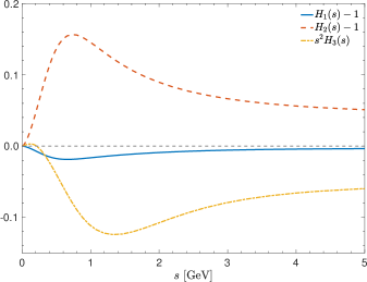
Figure 5: The deviations of the combinations $H_{1}(s^{2})$, $H_{2}(s^{2})$, and $s^{2}H_{3}(s^{2})$, defined in the Eq. (47), from their tree-level counterparts.

Next, we proceed to the full determination of $\overline{\Gamma}_{1}^{\,\rm sym}(s^{2})$ and $\overline{\Gamma}_{3}^{\,\rm asym}(q^{2})$ from the set of formulas given above [in particular Eqs. (20) and (24), together with Eqs. (46), (47) and (48)]. In order to accomplish this task, the functions $H_{1}(s^{2})$, $H_{2}(s^{2})$, and $s^{2}H_{3}(s^{2})$ must be computed from their defining equations, given in Eq. (47). This, in turn, requires the determination of the form factors $A_{1}(s^{2})$, $A_{3}(s^{2})$, and $A_{4}(s^{2})$, and the corresponding derivatives; since the impact of the unquenching effects on the ghost sector is expected to be rather small Ayala et al. (2012), for simplicity we use the quenched $A_{i}$ of Aguilar et al. (2019b). The final $H_{1}(s^{2})$, $H_{2}(s^{2})$, and $s^{2}H_{3}(s^{2})$ are shown in Fig. 5, for the symmetric configuration; similar results have been obtained for the asymmetric case (not shown).

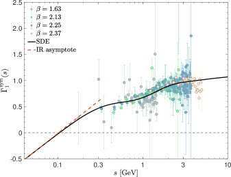
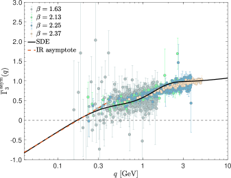
Figure 6: Left panel: The form factor of the three-gluon vertex in the symmetric configuration, $\overline{\Gamma}_{1}^{\,\rm sym}(s)$, obtained from lattice QCD (circles in different colors for each setup) and from the SDE-based approach (black continuous curve). Right panel: The same for the asymmetric form factor $\overline{\Gamma}_{3}^{\,\rm asym}(q)$. The IR asymptotes (red dashed lines) are given by Eqs. (49) and (50), respectively.

The comparison between the final SDE-based prediction for $\overline{\Gamma}_{1}^{\,\rm sym}(s^{2})$ and $\overline{\Gamma}_{3}^{\,\rm asym}(q^{2})$ and the corresponding unquenched lattice data is shown in Fig. 6; we observe a very good agreement for the entire range of momenta. It is rather evident that the particular shape of $J(q^{2})$, shown in the top right panel of Fig. 2 and given by Eq. (33), is largely responsible for the most characteristic features of the vertex form factor at intermediate and low momenta, namely its overall suppression with respect to its tree-level value, and the inevitable (albeit hard to observe) reversal of sign (zero crossing) in the deep IR.

It is clear that, due to the well-known ambiguities related with the scale setting Sommer (1994); Capitani et al. (1999); Becirevic et al. (1998); Boucaud et al. (2000), direct comparisons between quenched and unquenched data may be quantitatively subtle. Notwithstanding this caveat, the inclusion of quarks seems to moderate the amount of suppression with respect to Athenodorou et al. (2016). Specifically, the decrease observed between the renormalization point of $\mu=4.3$ GeV [where $\overline{\Gamma}^{\,\rm sym}_{1}(\mu^{2})=\overline{\Gamma}^{\,\rm asym}_{3}(\mu^{2})=1$] and a typical IR momentum, say $q_{{\scriptscriptstyle I\!R}}$=300 MeV, is given by $\overline{\Gamma}_{1}^{\rm sym}(q_{{\scriptscriptstyle I\!R}}^{2})$=0.47 and $\overline{\Gamma}_{1}^{\rm asym}(q_{{\scriptscriptstyle I\!R}}^{2})$=0.26, to be compared with $\overline{\Gamma}_{1}^{\rm sym}(q_{{\scriptscriptstyle I\!R}}^{2})$=0.33 and $\overline{\Gamma}_{1}^{\rm asym}(q_{{\scriptscriptstyle I\!R}}^{2})$=0.2 for the quenched case; thus, the observed suppression is reduced by about 25%. In addition, as expected from the corresponding displacement of $q_{0}$ at the level of the $J(q^{2})$ [see Sec. III.3, point (i)], the zero crossing of both vertex configurations occurs at momenta lower compared to the quenched case, in qualitative agreement with the analysis of Williams et al. (2016). In particular, we find that the zero crossing moves from about 150 MeV down to 105 MeV (symmetric case) and from roughly 240 MeV to about 170 MeV (asymmetric case).

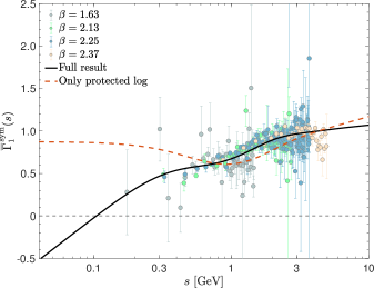
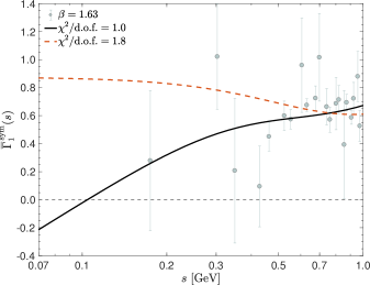
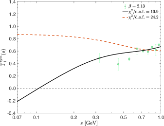
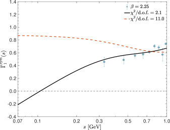
Figure 7: Top left plot: The effect of the unprotected logarithm of $J(q^{2})$ [see Eq. (33)] on the IR behavior of $\overline{\Gamma}_{1}^{\,\rm sym}(s)$. The black continuous line is $\overline{\Gamma}_{1}^{\,\rm sym}(s)$ derived using the full expression for $J(q^{2})$, given by Eq. (33). The red dashed curve represents the case where the massless logarithm, appearing in Eq. (33), is neglected. Top right plot: The $\chi^{2}/$d.o.f. when we compare the lattice data for $\beta=1.63$ with the results for $\overline{\Gamma}_{1}^{\,\rm sym}(s)$ with (black continuous) and without (red dashed) the unprotected logarithm. Bottom left plot: The same as the previous panel but for the lattice data with $\beta=2.13$. Bottom right plot: Same analysis, using the lattice data with $\beta=2.25$.

We next study in more detail the impact of the unprotected logarithm of $J(q^{2})$ on the IR behavior of the vertex. In particular, $\overline{\Gamma}_{1}^{\,\rm sym}(s^{2})$ is computed by plugging into Eq. (46) (i) the full $J(q^{2})$ given in Eq. (33) (black continuous curve), and (ii) a $J(q^{2})$ without the term $(1/6)\ln\left(q^{2}/\mu^{2}\right)$ (red dashed curve). As we can see in the top left panel of Fig. 7, for momenta below $800$ MeV the unprotected logarithm starts to dominate the behavior of $\overline{\Gamma}_{1}^{\,\rm sym}(s^{2})$, forcing not only its suppression but also its IR divergence. In the remaining panels of Fig. 7 we show that the three sets of lattice data considered exhibit individually a clear preference for case (i); in fact, even in the least favorable case (top right panel), where the data are rather sparse and with sizable errors, the $\chi^{2}/$d.o.f. is $1.8$ times smaller than that of case (ii).

Finally, turning to the transverse part of $\Gamma_{\alpha\mu\nu}$, it is clear that the corresponding form factors ought to be determined from a detailed SDE study, which is still pending. In fact, the good coincidence found between the SDE-based prediction [with $Y_{1}(s^{2})=Y_{4}(s^{2})=0$] and the lattice must be interpreted with caution, especially in view of the sizable errors assigned to the data. Indeed, given the present precision, one may easily envisage how reasonably sized transverse contributions could be rather comfortably accommodated, provided they follow the general trend of the data. We hope to report progress in this direction in the near future.

IV.4 Effective couplings

It is rather instructive to study how the suppression of the three-gluon vertex manifests itself at the level of a typical renormalization-group invariant quantity, which is traditionally used to quantify the effective strength of a given interaction.

To that end, we next consider the two effective couplings related to $\overline{\Gamma}_{1}^{\,\rm sym}(s^{2})$ and $\overline{\Gamma}_{3}^{\,\rm asym}(q^{2})$, to be denoted by ${\widehat{g}}^{\,\rm sym}(s^{2})$ and ${\widehat{g}}^{\,\rm asym}(q^{2})$, respectively. In particular, following standard definitions Athenodorou et al. (2016); Mitter et al. (2015); Fu et al. (2019), we have

$${\widehat{g}}^{\,\rm sym}(s^{2})=g^{\,\rm sym}(\mu^{2})\,s^{3}\,\overline{\Gamma}_{1}^{\,\rm sym}(s^{2})\Delta^{3/2}(s^{2})\,,\qquad{\widehat{g}}^{\,\rm asym}(q^{2})=g^{\,\rm asym}(\mu^{2})\,q^{3}\,\overline{\Gamma}_{3}^{\,\rm asym}(q^{2})\Delta^{3/2}(q^{2})\,.$$ (52)

We emphasize that these two couplings may be recast in the form

$${\widehat{g}}^{\,\rm sym}(s^{2})=s^{3}\frac{T^{\,\rm sym}(s^{2})}{\Delta^{3/2}(s^{2})}\,,\qquad{\widehat{g}}^{\,\rm asym}(q^{2})=q^{3}\,\frac{T^{\,\rm asym}(q^{2})}{\Delta(0)\Delta^{1/2}(q^{2})}\,,$$ (53)

thus making contact with the corresponding definitions employed within the MOM schemes Alles et al. (1997); Boucaud et al. (1998). Turning to their computation, we use for the ingredients entering in the above definitions both lattice data as well as the corresponding SDE-derived quantities; the results obtained are displayed in Fig. 8.

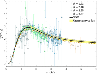
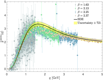
Figure 8: Left panel: The symmetric effective coupling, ${\widehat{g}}^{\,\rm sym}(s)$, defined in Eq. (52), obtained using the lattice data (full circles) and the results of the SDE-based approach (black continuous line). The yellow band represents how the SDE result for ${\widehat{g}}^{\,\rm sym}(s)$ changes when the value of $g$ at $\mu$=4.3 GeV has an uncertainty of $\pm 5\%$, with central values $g^{\,\rm sym}(\mu^{2})=1.86$ [$\alpha^{\,\rm sym}(\mu^{2})=0.27$]. Right panel: The same for the asymmetric effective coupling, ${\widehat{g}}^{\,\rm asym}(q^{2})$, with a central value $g^{\,\rm asym}(\mu^{2})=2.16$ [$\alpha^{\,\rm asym}(\mu^{2})=0.37$].

It is interesting to carry out a direct comparison of the effective coupling, ${\widehat{g}}^{\,\rm sym}(s^{2})$, with the corresponding quantity, ${\widehat{g}}_{\rm gh}^{\,\rm sym}(s^{2})$, associated with the ghost-gluon vertex in the symmetric configuration. Specifically,

$${\widehat{g}}_{\rm gh}^{\,\rm sym}(s^{2})=g^{\,\rm sym}(\mu^{2})\,s\,\overline{B}_{1}^{\,\rm sym}(s^{2})F(s^{2})\Delta^{1/2}(s^{2})\,,$$ (54)

where $\overline{B}_{1}^{\,\rm sym}(s^{2})$ denotes the form factor proportional to the tree-level component of the ghost-gluon vertex, renormalized at the same MOM point, $\mu=4.3$ GeV. The functional form used for $\overline{B}_{1}^{\,\rm sym}(s^{2})$ has been obtained from the analysis of Aguilar et al. (2019b) and it is shown in the left panel of Fig. 9. The two couplings are displayed in the left panel of Fig. 10; clearly, as the momentum $s$ decreases, ${\widehat{g}}^{\,\rm sym}(s^{2})$ becomes considerably smaller than ${\widehat{g}}_{\rm gh}^{\,\rm sym}(s^{2})$.

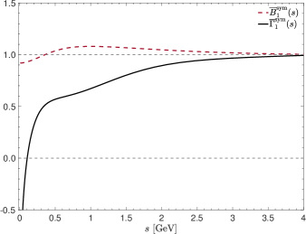
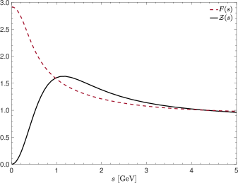
Figure 9: Left panel: $\overline{\Gamma}_{1}^{\,\rm sym}(s)$ (black continuous line) compared with the form factor $\overline{B}_{1}^{\,\rm sym}(s)$ of the ghost-gluon vertex (red dashed curve), in the symmetric configuration. Right panel: The gluon and ghost dressing functions, ${\cal Z}(s)$ and $F(s)$, respectively.

In order to analyze in detail the origin of this relative suppression, it is advantageous to introduce the gluon dressing function, ${\cal Z}(q^{2})$, defined as ${\cal Z}(q^{2})=q^{2}\Delta(q^{2})$, which is shown on the right panel of Fig. 9, together with the corresponding quantity for the ghost propagator, $F(q^{2})$, introduced in Eq. (2). Then, the two effective couplings assume the form

$${\widehat{g}}^{\,\rm sym}(s^{2})=g^{\,\rm sym}(\mu^{2})\,\overline{\Gamma}_{1}^{\,\rm sym}(s^{2}){\cal Z}^{3/2}(s^{2})\,,\qquad{\widehat{g}}_{\rm gh}^{\,\rm sym}(s^{2})=g^{\,\rm sym}(\mu^{2})\,\overline{B}_{1}^{\,\rm sym}(s^{2})F(s^{2}){\cal Z}^{1/2}(s^{2})\,.$$ (55)

We next consider the ratio of these two couplings,

$${\cal R}_{g}(s^{2})={\widehat{g}}^{\,\rm sym}(s^{2})/{\widehat{g}}_{\rm gh}^{\,\rm sym}(s^{2})=\underbrace{\left[{\cal Z}(s^{2})/F(s^{2})\right]}_{{\cal R}_{2}(s^{2})}\underbrace{\left[\overline{\Gamma}_{1}^{\,\rm sym}(s^{2})/\overline{B}_{1}^{\,\rm sym}(s^{2})\right]}_{{\cal R}_{3}(s^{2})}\,,$$ (56)

where the partial ratios ${\cal R}_{2}(s^{2})$ and ${\cal R}_{3}(s^{2})$ quantify the relative contribution from the two- and three-point sectors, respectively, at the various momentum scales involved. The three ratios, ${\cal R}_{g}(s^{2})$, ${\cal R}_{2}(s^{2})$, and ${\cal R}_{3}(s^{2})$ are shown on the right panel of Fig. 10.

Interestingly, ${\cal R}_{2}(s^{2})$ and ${\cal R}_{3}(s^{2})$ are smaller than $1$ for $s<880$ MeV and $s<4.3$ GeV, respectively. Therefore, in the region of momenta between $(0-880)$ MeV, the suppression of ${\widehat{g}}^{\,\rm sym}(s^{2})$ emerges as a combined effect of both the two- and the three-point sectors, whereas, from $880\,\mbox{MeV}$ to $2.4\,\mbox{GeV}$ the suppression is exclusively due to the behavior of the three-gluon vertex.

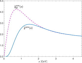
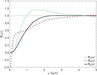
Figure 10: Left panel: The comparison of the effective couplings, ${\widehat{g}}^{\,\rm sym}(s)$ (blue solid line) and ${\widehat{g}}_{\rm gh}^{\,\rm sym}(s)$ (magenta dashed), defined from the three-gluon vertex, Eq. (52), and from the ghost-gluon vertex, Eq. (54), respectively. Right panel: The ratios ${\cal R}_{g}(s)$ (black continuous), ${\cal R}_{2}(s)$ (green dotted), and ${\cal R}_{3}(s)$ (red dashed) introduced in the Eq. (56).

V Discussion and Conclusions

In this article we have considered several nonperturbative aspects related to the gluon propagator, $\Delta(q^{2})$, and the three-gluon vertex, $\Gamma_{\alpha\mu\nu}$, in the context of Landau gauge QCD with $N_{f}$=2+1 dynamical quarks. Our approach combines a SDE-based analysis, carried out within the PT-BFM framework, with new data gathered from lattice QCD simulations with $N_{f}$=2+1 domain wall fermions. In particular, from the SDE point of view, the gluon kinetic term $J(q^{2})$ has been computed indirectly, by obtaining $m^{2}(q^{2})$ from its own “gap equation” and then “subtracting” it from the new lattice data for $\Delta^{-1}(q^{2})$. The $J(q^{2})$ so determined is subsequently used for the “gauge technique” reconstruction (BC solution) of certain key form factors of $\Gamma_{\alpha\mu\nu}$, evaluated at two special kinematic configurations (“symmetric” and “asymmetric”). The two main quantities emerging from this construction, denoted by $\overline{\Gamma}_{1}^{\rm sym}(s^{2})$ and $\overline{\Gamma}_{3}^{\rm asym}(q^{2})$, are then compared with recently acquired lattice data, displaying very good coincidence. We emphasize that, while the determination of $J(q^{2})$ hinges on the use of the lattice data for the gluon propagator, the subsequent results derived by means of this $J(q^{2})$ constitute genuine theoretical predictions.

There are certain key theoretical notions underlying this work which are worth highlighting.

(i) The recent nonlinear SDE analysis of Aguilar et al. (2019c) generalizes from pure Yang-Mills to the case of real-world QCD with dynamical quarks, giving rise to a $m^{2}(q^{2})$ that displays all qualitative features known from the quenched case.

(ii) The low-momentum behavior of $J(q^{2})$ is clearly dominated by the unprotected logarithm originating from the ghost loop. In a pure Yang-Mills context, the diverging contribution of this logarithm overcomes the opposing action of its protected counterparts, leading to the IR suppression of $J(q^{2})$ and its zero crossing. The inclusion of quark loops, which are regulated by the quark masses, gives rise to additional IR finite contributions, whose net effect is to attenuate the aforementioned outstanding features.

(iii) By virtue of the fundamental STI of Eq. (29), the longitudinal form factors of $\Gamma_{\alpha\mu\nu}$ display the same qualitative characteristics as the $J(q^{2})$; in that sense, the influence of the ghost sector, and in particular of the ghost-gluon kernel, is rather limited, and does not alter the main dynamical properties that $\overline{\Gamma}_{1}^{\rm sym}(s^{2})$ and $\overline{\Gamma}_{3}^{\rm asym}(q^{2})$ inherit from the $J(q^{2})$.

(iv) In our opinion, the present analysis provides additional support for the picture of the IR sector of (Landau gauge) QCD that has emerged in recent years, according to which, quarks and gluons acquire dynamically generated masses, while the ghosts remain strictly massless Aguilar et al. (2008); Boucaud et al. (2008); Fischer et al. (2009); Cloet and Roberts (2014); Binosi et al. (2015). The three-gluon vertex appears to be the host of an elaborate synergy between the mechanisms responsible for this exceptional mass pattern, thus providing an outstanding testing ground both for physics ideas as well as computational methods.