Towards comprehension of the variability of the magnetic chemically peculiar star CU Virginis (HD 124 224)

Abstract

The upper main sequence stars CU Virginis is the most enigmatic object among magnetic chemically peculiar (mCP) stars. It is an unusually fast rotator showing strictly periodic light variations in all regions of the electromagnetic spectrum, as well as spectroscopic and spectropolarimetric changes. At same time, it is also the first radio main-sequence pulsar. Exploiting information hidden in phase variations, we monitored the secular oscillation of the rotational period during the last 53 years. Applying own phenomenological approach, we analyzed 37 975 individual photometric and spectroscopic measurements from 72 data sources and improved the O-C model. All the relevant observations indicate that the secular period variations can be well approximated by the fifth degree polynomial.

¹Department of Theoretical Physics and Astrophysics, Masaryk University, Kotlářská 2, CZ 611 37 Brno, Czech Republic; mikulas@physics.muni.cz

²Astronomical Institute, University of Wrocław , Wrocław, Poland

³Center of Excellence in Information Systems, Tennessee State University, Nashville, Tennessee, USA

1 Introduction

Magnetic chemically peculiar (mCP) stars are the most suitable test beds for studying rotation and its variation in the upper (B2V to F6V) main-sequence stars. The surface chemical composition of these objects uses to be very uneven. Overabundant elements are, as a rule, concentrated into large spots persisting there for decades to centuries. The abundance unevenness of the atmospheres influences the stellar spectral energy distribution. As the star rotates, periodic variations in the spectrum, brightness, and longitudinal magnetic field are observed. We have studied both present and archival observations of all kinds to check the stability of the rotation periods of mCP stars.

The changes rotation periods were derived from shifts of (light, phase) phase curves by means of the method developed by Mikulášek et al. (2008). They applied this method at first to the helium strong star V901 Ori. Then, it was many times improved and tested on mCPs and other types of variables (see, e.g. Mikulášek 2015). The method is based on the usage of suitable phenomenological models of phase curves of rotation tracers and the period variation (one can find a detailed manual in Mikulášek 2016). Solution through robust regression provides us with all model parameters and estimations of their uncertainty.

The vast majority of CP stars studied to date display strictly constant rotational periods. However, a few mCP stars, including CU Vir and V901 Ori, have been discovered to exhibit rotational period variations caused by yet unknown reasons.

2 Period variations of CU Virginis

CU Vir = HD 124224, is a bright, rapidly-rotating ($\overline{P}=0.520694$ d), medium-aged silicon mCP star (Kochukhov & Bagnulo 2006). It is also the first known main-sequence stellar radio pulsar (Trigilio et al. 2000, and references therein). Pyper et al. (1998), using their new and archival photometry, constructed an O-C diagram showing a sudden period increase of 2.6 s (slower rotation) in 1984! Another smaller jump toward a longer period in 1998 was reported by Pyper & Adelman (2004). Mikulášek et al. (2011a) processed all available measurements of CU Vir and found that its rotation was gradually slowing until 2005 and since then has been accelerating.

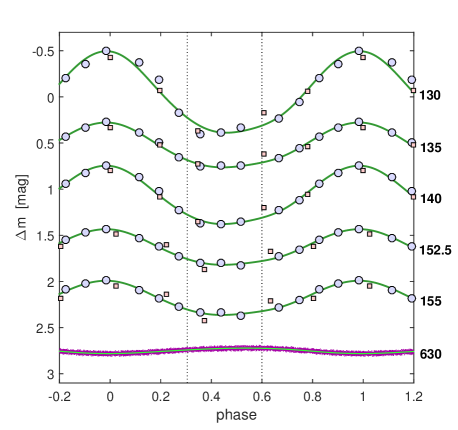
Figure 1.: Comparison of light curves in far UV and red regions of CU Vir spectrum. Blue circles and red squares denote magnitudes derived from IUE and HST spectra, violet points are the measurements from SMEI satellite. Wavelengths are expressed in nanometers and phases are calculated using ephemeris (3). Green lines are the fits of the light curve phenomenological model, assuming two symmetric photometric spots with centers at the phases 0.303 and 0.598 (black dotted lines).

2.1 Models of phase function and period

The first attempts to describe and model the apparent changes of the rotation period of CU Vir was based on the assumption that period changes (Pyper et al. 1998; Pyper & Adelman 2004), which can be represented as a series of linear fragments in the O-C/phase shift diagrams. The possible physics of abrupt changes was afterward discussed in Stȩpień (1998).

Mikulášek et al. (2011a) showed that the change of the period is more likely gradual, without any jumps. The phase function (sum of phase and epoch) $\vartheta(t)$ was in their paper approximated by an aperiodic, three-parametric, symmetric biquadratic function, resembling a segment of a simple cosine function.

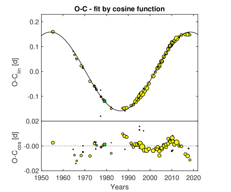
Figure 2.: Upper: $\textit{O-C}_{\rm{lin}}$ versus time in years, where $O$ is the moment of the zero phase and $C_{\rm{lin}}=M_{0}+P_{0}\times E$, where $M_{0},\,P_{0}$ are the parameters described in Sect. 1, and $E$ is the number of rotational cycles elapsed from the initial epoch $M_{0}$. Inconstancy of $\textit{O-C}_{\rm{lin}}$ is the result of rotation period $P$. $\textit{O-C}_{\rm{lin}}$ is fitted by a four parametric cosine function. Bottom: The residuals $\textit{O-C}_{\cos}$ show apparent undulations. Optical photometry – yellow circles, UV spectrophotometry - green squares, red circles – equivalent widths (EWs) of He i lines, black ones – Si ii, violet ones – H i, blue – effective magnetic field, and cyan – radial velocity measurements. The size of symbols is are proportional to adopted weights.

Krtička et al. (2017) showed that cyclic oscillations in the rotational period revealed by Mikulášek et al. (2011a) might result from the interaction of the internal magnetic field and differential rotation and predict a rotational cycle timescale of 51 yr. In that sense, we first used the model assuming periodic variations of the period $P(t)$ and phase function $\vartheta(t)$ with the period $\mathit{\Pi}$. Using all 18 267 observations of CU Vir  available up to 2015, we found the period $\mathit{\Pi}=67.6(5)$ yr, close to the theoretical prediction.

Adopting all data known by the end of 2016 (especially those of Pyper et al. 2013), Mikulášek (2016) applied this model again in the following form:

$$\displaystyle\vartheta_{1}(t)=\frac{t-M_{0}}{P_{0}};\quad\phi(t)=\frac{t-T_{0}}{\mathit{\Pi}};\quad\Delta(\phi)=-\frac{A}{P_{0}}\cos\left(2\,\pi\phi\right);\quad\vartheta=\vartheta_{1}-\Delta(\phi);$$ (1)

$$\displaystyle\theta(\vartheta)=M_{0}+P_{0}\,\vartheta+P_{0}\,\Delta(\phi);\quad P(t)=P_{0}\frac{\mathrm{d}\vartheta_{1}}{\mathrm{d}\vartheta}\doteq P_{0}\left[1+\frac{2\,\pi\,A}{\mathit{\Pi}}\,\sin\left(2\,\pi\,\phi(t)\right)\right],$$

where $\Delta$ is an auxiliary function, $A$ is a semiamplitude of O-C changes with the minimum at $T_{0}$ and the semiamplitude of the mean period undulation being $A_{\mathrm{P}}=2\,\pi AP_{0}/\mathit{\Pi}$. $M_{0}$ was chosen so that $\Delta(\tilde{\vartheta_{0}}=0)=\mathrm{d}\Delta/\mathrm{d}\vartheta_{0}=0$. Analysing all the available observational data of CU Vir, we found $M_{0}=2\,446\,604.4390$ (fixed), $P_{0}=0.520\,694\,04(3)$ d. $T_{0}=2\,446\,604(13),\ \mathit{\Pi}=24\,110(150)\,\mathrm{d}=66.0\pm 0.4$ yr, $A=0.1611(5)$ d, and $A_{\mathrm{P}}=1.888$ s. The data (19 641 individual observations) cover more than one cycle of the proposed sinusoidal variations.

At the same time Mikulášek (2016) modeled the data using polynomial model of the phase function $\vartheta(t)$ and found that fourth order polynomial model (5 parameters) gave a bit better results than the harmonic one. The application of the fifth order polynomial (6 parameters) has occurred being unsubstantiated.

3 Recent results

3.1 New observation

Recently, the volume of the photometric data of CU Vir has been increased by the space photometry made in the years 2003-2011 by the Solar Mass Ejection Imager (SMEI) experiment (Eyles et al. 2003; Jackson et al. 2004). The photometry, available through the University of California San Diego web page has been processed to remove the instrumental effects. The corrections included subtraction of the repeatable seasonal variability, and subsequent rejoection of outliers and detrending. In effect, we obtained 19226 individual photometric observations for further analysis.

During 2017-8 we obtained 10 new spectrograms taken by far UV spectrograph on board Hubble Space Telescope. We yielded 25 magnitudes in 5 passbands centered at 130, 135, 140, 152.5, and 155 nm. In addition, we derived 55 new magnitudes from 11 spectrograms taken by IUE. Phased light curves of all above mentioned data are depicted in Fig. 1. 689 high-precision BV measurements acquired by one of us (GH) with the Automated Photometric Telescope (APT) at Fairborne Observatory in Arizona at 2017 and 2018 seasons harbored our CU Vir data in the present.

Presently, we have in our disposal altogether 37 975 relevant observations of CU Vir covering sufficiently the time interval 1955-2018. The prevailing source of information is the photometry with 37 313 measurements done/derived in the filters with the centers in the interval of 135–765 nm. The other tracers which allow to monitor period changes are measurements of equivalent widths of He i, Si ii, and H i lines (569), effective magnetic field (59), and radial velocities (59). The present data are rich enough to improve the model of the phase function.

3.2 Discussion of phase function models

First, we applied the simple four-parametric cosine phase function model described by relations (1), used in Krtička et al. (2017) and Mikulášek (2016). The found model parameters were slightly, but significantly shifted versus those ones found before: $P_{0}=0.520\,693\,87(2)$ d, $A=-0.1587(3)$ d, $T_{0}=2\,446\,573(2)$, and $\mathit{\Pi}=23\,370(90)\,\mathrm{d}=64.2(3)$ yr. The quality of the O-C fit can be quantified by the relative $\chi^{2}_{r}$, where we found unacceptably high value of 28.

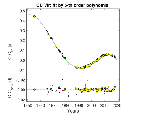
Figure 3.: Upper: $O-C_{\rm{lin}}$ ($C_{\rm{lin}}=M_{01}+P_{1}\times E$, where $M_{01},\,P_{1}$ are the parameters of the linear approximation, see in Sect. 3.2, and $E$ is the number of rotational cycles elapsed from the initial epoch $M_{01}$) versus time in years fitted by fifth-order polynomial phenomenological model. Bottom: The residuals $\textit{O-C}_{\rm{pol5}}$ (see Eq. (3.2)) show only a weak undulation. The symbols are the same as in Fig. 2.

The detailed inspection of O-C diagram (Fig. 2) shows that the cosine model can be regarded only as the first approximation of the reality. As the $\textit{O-C}_{\cos}$ exhibits apparent double wave during the cycle of 65 years, we conclude that it is necessary to raise the number of free parameters describing the phase function model by at least two. It suggests itself the usage of the second-order harmonic polynomial or the fifth-order polynomial ($N=5$). Although the first possibility is permitted by theory (Krtička et al. 2017), we shall discuss the second one which is less biased.

$$\displaystyle\vartheta_{1}=\frac{t-M_{01}}{P_{1}},\quad\theta_{1}=\frac{\vartheta_{1}}{10^{4}},\quad\displaystyle\theta=\frac{\vartheta}{10^{4}},\quad\frac{\mathrm{d}\theta}{\mathrm{d}\vartheta}=\frac{\mathrm{d}\theta_{1}}{\mathrm{d}\vartheta_{1}}=10^{-4},$$ (2)

$$\displaystyle\vartheta(\vartheta_{1})=\vartheta_{1}+\sum_{i=2}^{N}\alpha_{i}\,\left(\theta_{1}^{i}+\sum_{j=0}^{i-1}\beta_{ij}\theta_{1}^{j}\right),$$

$$\displaystyle T(\vartheta)\doteq M_{01}+P_{1}\vartheta-P_{1}\,\sum_{i=2}^{N}\alpha_{i}\,\left(\theta^{i}+\sum_{j=0}^{i-1}\beta_{ij}\theta^{j}\right)$$

$$\displaystyle P(t)=\frac{\mathrm{d}t}{\mathrm{d}\vartheta}=P_{1}\left(\frac{\mathrm{d}\vartheta}{\mathrm{d}\vartheta_{1}}\right)^{-1}\doteq P_{1}\left[1-\frac{\mathrm{d}\theta_{1}}{\mathrm{d}\vartheta_{1}}\sum_{i=2}^{N}\alpha_{i}\left(i\,\theta_{1}^{i-1}+\sum_{j=1}^{i-1}j\,\beta_{ij}\,\theta_{1}^{j-1}\right)\right],$$

$$\displaystyle P(\vartheta)=\frac{\mathrm{d}T}{\mathrm{d}\vartheta}\doteq P_{1}\left[1-\frac{\mathrm{d}\theta}{\mathrm{d}\vartheta}\sum_{i=2}^{N}\alpha_{i}\left(i\,\theta^{i-1}+\sum_{j=1}^{i-1}j\,\beta_{ij}\,\theta^{j-1}\right)\right],$$

$$\displaystyle\dot{P}(t)=\frac{1}{P_{1}}\frac{\mathrm{d}P}{\mathrm{d}\vartheta_{1}}=-\left(\frac{\mathrm{d}\theta_{1}}{\mathrm{d}\vartheta_{1}}\right)^{\!2}\sum_{i=2}^{N}\alpha_{i}\left[(i^{2}\!-\!i)\,\theta_{1}^{i-2}+\sum_{j=2}^{i-1}(j^{2}\!-\!j)\,\beta_{ij}\,\theta_{1}^{j-2}\right],$$

where $M_{01}=2\,452\,652.9973(6),P_{1}=0.520\,703\,479(14)$ d are ephemeris of the linear approximation $(N=1)$. For $N=5$, $\alpha_{2}=0.12069(19)$, $\alpha_{3}=-0.02914(18)$, $\alpha_{4}=-0.03039(14)$, $\alpha_{5}=-0.00223(15)$ are the dimensionless parameters founded iteratively by weighted robust regression (for details see Mikulášek 2016). Rightfulness of the highest order of the polynomial follows from the fact that $|\alpha_{5}|/\delta\alpha_{5}=15$. Coefficients $\beta_{20}=0.52219$, $\beta_{21}=-1.0691,\ \beta_{30}=0.82694,\ \beta_{31}=0.88898,\ \beta_{32}=-2.6527,\ \beta_{40}=0.34705,$ $\beta_{41}=3.0039,\ \beta_{42}=-0.97123,\ \beta_{43}=-3.771,\ \beta_{50}=-0.96466,\ \beta_{51}=2.1025,$ $\beta_{52}=6.2491,\ \beta_{53}=-3.362,$ and $\beta_{54}=-4.8325$ are orthogonalization parameters found by operations described in Mikulášek (2016).

4 Conclusions

Although $\chi^{2}_{r}=7$ of the fit of the polynomial is four times smaller than for the cosine one, its high value shows that the 5-th order polynomial fit is unable to describe observed tiny changes on the time scale of several years - see Fig. 3. Nevertheless, the last global model represents a substantial improvement with respect to the previous models and leads us to a better comprehension of variability of the rotation period of CU Vir.

Acknowledgments

This research was supported by grant GA ČR 16-01116S. This research was partly based on the IUE data derived from the INES database using the SPLAT package. AP acknowledges the support from the National Science Centre grant no. 2016/21/B/ST9/01126.

References

- Eyles et al. (2003) Eyles, C.J., Simnett, G.M., Cooke, M.P., Buffington, A, et al. 2003, Solar Physics, 217, 319
- Jackson et al. (2004) Jackson, B.V., Buffington, A., Hick, et all, M. 2004, Solar Physics, 225, 177
- Kochukhov & Bagnulo (2006) Kochukhov, O. & Bagnulo, S. 2006, ApJ, 726, 24
- Krtička et al. (2017) Krtička, J., Mikulášek, Z., Henry, G. W., Kurfürst, P., & Karlický, M. 2017, MNRAS, 464, 933
- Mikulášek (2015) Mikulášek, Z. 2015, A&A, 584, A8
- Mikulášek (2016) Mikulášek, Z. 2016, CAOSP, 46, 95
- Mikulášek et al. (2008) Mikulášek, Z., Krtička, J., Henry, G. W., Zverko, J., Žižňovský, J. et al. 2008, A&A, 485, 585
- Mikulášek et al. (2011a) Mikulášek, Z., Krtička, J., Henry, G. W. et al. 2011a, A&A, 534, L5
- Mikulášek et al. (2011b) Mikulášek, Z., Krtička, J., Janík J. et al. 2011b, in Magnetic Stars, Proceedings of the International Conference, SAO RAS 2010, eds: I. I. Romanyuk and D. O. Kudryavtsev, 52
- Mikulášek et al. (2014) Mikulášek, Z., Krtička, J., Janík, J., Zejda, M., Henry, G. W., Paunzen, E., Žižňovský J., & Zverko, J. 2014, in Putting A Stars into Context: Evolution, Environment, and Related Stars, ed. G. Mathys, E. Griffin, O. Kochukhov, R. Monier, G. Wahlgren, 270
- Mikulášek et al. (2007a) Mikulášek, Z., Krtička, J., Zverko, J., Žižňovský, J., & Janík, J. 2007, in ASP Conf. Ser. 361, Active OB-Stars: Laboratories for Stellar and Circumstellar Physics, ed. S. Štefl, S. P. Owocki, & A. T. Okazaki, 466
- Mikulášek & Zejda, (2013) Mikulášek, Z. & Zejda, M., in Úvod do studia proměnných hvězd, ISBN 978-80-210-6241-2, Masaryk University, Brno 2013
- Mikulášek et al. (2007b) Mikulášek, Z., Zverko, J., Krtička, J. et al. 2007, in Physics of Magnetic Stars, Proceedings of the International Conference, SAO RAS 2010, eds: I. I. Romanyuk and D. O. Kudryavtsev, Special Astrophysical Observatory, 300
- Pyper & Adelman (2004) Pyper, D. M., & Adelman, S. J. 2004, The A-Star Puzzle, IAU Symposium No. 224, ed s. J. Zverko, J. Žižňovský, S. J. Adelman, & W. W. Weiss (Cambridge University Press, Cambridge), 307
- Pyper et al. (1998) Pyper, D. M., Ryabchikova, T., Malanushenko, V. et al. 1998, A&A, 339, 822
- Pyper et al. (2013) Pyper D. M., Stevens, I. R., & Adelman S. J., 2013, MNRAS, 431, 2106
- Stȩpień (1998) Stȩpień, K.: 1998, A&A, 337, 754
- Trigilio et al. (2000) Trigilio, C., Leto, P., Leone, F., Umana, G., & Buemi, C. 2000, A&A, 362, 281