Erratum: Nonlinear spherical perturbations in quintessence models of dark energy

1 Introduction

We reported results of our study on non-linear spherical perturbations in quintessence models of dark energy. In the process of some follow up studies we discovered that a scaling factor in the code used for numerical calculations that should have been set to unity was set to a large value ($10^{3}$). Thus the scale of perturbations was much larger than intended, and for the larger scales the amplitude of dark matter perturbations was much higher than realistic. We provide corrected results here in this erratum. We find that there is no change in the perturbations for dark matter. The amplitude of perturbations in dark energy is much smaller than presented in the paper [1]. Same holds true for spatial variation in the equation of state parameter.

Our key conclusions do not change.

• Dark energy perturbations do not lead to any variation in dark matter perturbations, e.g., radius at turn around and the virial radius, as well as density contrast at these two epochs remains unchanged.

• Dark energy perturbations grow at the linear rate, or faster.

• Dark energy perturbations remain small at all times and scales in response to non-linear dark matter perturbations.

• Equation of state parameter $w$ becomes a function of scale and the variation is related to the density contrast in dark matter.

• Gradients in dark energy and metric coefficients are strongly suppressed.

We find that two of the approaches discussed and discarded in the original paper do not work properly with the correct scaling. This is described in some detail.

For completeness, we give here the corrected figures, where the incorrect scaling factor in the code gave us incorrect variation. Note: We have indexed the figures in this erratum to have same figure numbers as in original article [1]. Two extra figures are added to compliment figure 8 and 13, these are labeled as figure 8(extra) and figure 13(extra), respectively.

2 Dark energy in over dense profile

The initial profile for dark matter perturbation is taken to be(see section 2.0.1 of article [1] for details):

$$\delta_{i}(r)=\left\{\begin{array}[]{lll}\alpha_{0}\left[1-\left(\frac{r}{\sigma_{0}}\right)^{2}\right]^{2}-\alpha_{1}\left[1-\left(\frac{r}{\sigma_{1}}\right)^{2}\right]^{2}&}{&\left(r\leq\sigma_{0}\right)\\ -\alpha_{1}\left[1-\left(\frac{r}{\sigma_{1}}\right)^{2}\right]^{2}&}{&\left(\sigma_{0}<r\leq\sigma_{1}\right)\\ 0&}{&\left(r>\sigma_{1}\right)\\ \end{array}\right.$$ (2.1)

For the over dense case the scales used are small ($\sigma_{0}=3,\sigma_{1}=18$, $(3,18)$) and hence dark energy perturbations are very weak. The claim that spatio-temporal fluctuations develop in dark energy continue to hold, though the amplitude of these fluctuations is much smaller than was reported earlier. This is very clear for the under dense case which has a larger scale: we had shown that dark energy perturbations at larger scales develop a larger amplitude for the same amplitude of dark matter perturbations.

We find that after the corrections, dark energy perturbations are very small at small scales, e.g. for $(3,18)$ mentioned above. Thus we supplement the corrected figures with results for a super cluster size halo with two length parameters as $(30,75)$ Mpc(figures in 8(extra)). This case shows a clear evolution of spatio-temporal perturbations. Density contrast in dark energy at different redshifts is shown in fig 8.

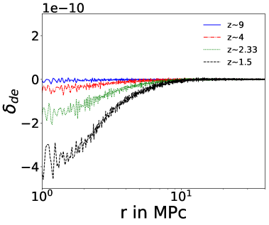
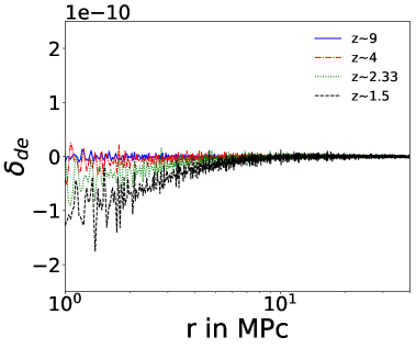
Figure 8: Density contrast for dark energy as a function of scale at different epochs. We see that the amplitude of perturbations in dark energy remains small at all scales and at all times. The left panel is for $V\propto\psi^{2}$ while the right panel is for $V\propto\exp(-\psi)$.

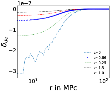
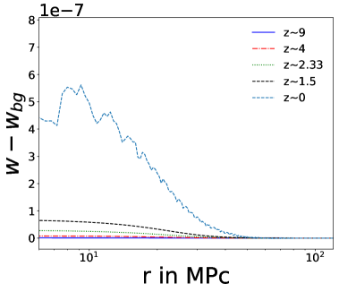
Figure 8(extra): Density contrast for dark energy for a super cluster sized perturbation collapsing around $z\simeq 0.02$.

Evolution of the equation of state for dark energy $w$ is shown in 9. We have plotted the difference between the value of $w$ and the expected value in the background model, taken here to be the value at large scales in the simulation. We can see that the fluctuations are non-zero but very small.

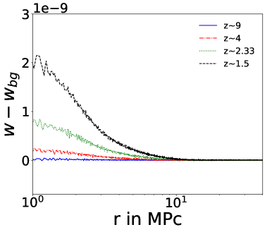
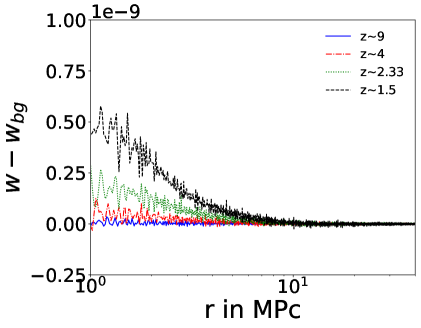
Figure 9: The equation of state parameter for dark energy as a function of scale at different epochs.

3 Dark Energy in under dense regions

We present the variation of density contrast for dark energy and the equation of state parameter $w$ in figures 10 and 11. The amplitude of fluctuations is much smaller than presented in the original work. The variation of $w$ with time is much more significant than the spatial variation.

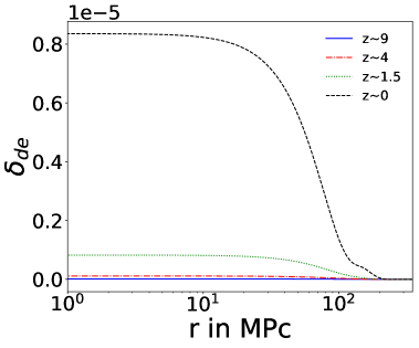
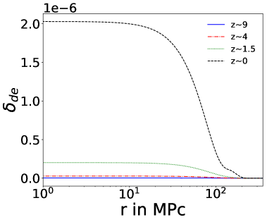
Figure 10: Density contrast for dark energy as a function of scale $r$ for a matter under-density from simulation UD1. This is plotted at multiple epochs. We find that dark energy perturbations grow but the amplitude remains small in absolute terms. The left panel is for $V\propto\psi^{2}$ while the right panel is for $V\propto\exp(-\psi)$.

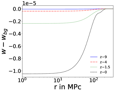
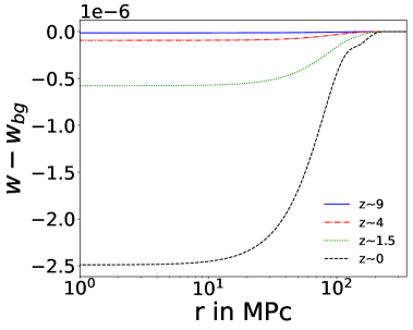
Figure 11: Equation of state parameter $w$ as a function of scale $r$ for a void, i.e., a matter under-density for simulation UD1. This is plotted at multiple epochs. We find that $w$ inside the void is smaller than at large scales. The left panel is for $V\propto\psi^{2}$ while the right panel is for $V\propto\exp(-\psi)$.

4 Comparison with linear theory

The conclusion presented in article that nonlinear perturbations at later times grow faster than linear ones continues to hold for corrected scales. The correspondence between growth rate of $\delta_{dm}(1+w)$ and growth rate of $\delta_{de}$ holds through and is similar as simulated earlier. The corrected variation is presented in fig 12.

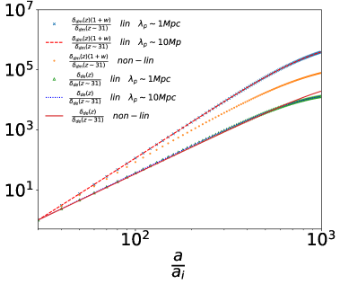
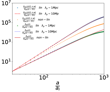
Figure 12: A comparison of the evolution of dark energy perturbations. Left panel is for $V\propto\psi^{2}$ while right one are for $V\propto\exp(-\psi)$. At very large scales the linear theory prediction for the magnitude of dark energy perturbations scales as $(1+w)\delta_{dm}$. We have plotted this combination for linearly evolved $\delta_{dm}$ for two scales: $1$ Mpc (cross) and $10$ Mpc (dashed line). Linear evolution of dark energy density contrast for the two scales is also shown here as triangles ($1$ Mpc) and dotted line ($10$ Mpc). We find that the linear evolution for dark energy perturbations is slower at small scales as compared to the expected variation at large scales. All points pertaining to linear evolution are normalised to unity at the left corner.

5 Role of spatial gradient in field dynamics

In this context the results as reported in fig 13 of [1] holds and here we plot the graph with corrected scales in fig (13).

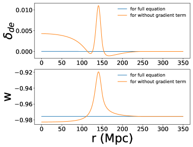
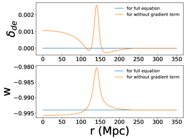
Figure 13: In this figure we explore the leading cause of variation of equation of state parameter $w$ for simulation UD1. We show the variation computed by retaining only the local Hubble expansion terms in the equation of motion and compare it with the full simulation. In the former case, we ignore the gradient term. We find that the variation of $w$ is fairly strong and has some localised features when the gradient terms are ignored. The localised features are not present in the full simulation indicating that the gradients of the scalar field are suppressed in the evolution, and the local Hubble expansion is not the only determining factor. This result remains valid after correction in the scale, though with a reduced amplitude of fluctuations.

6 Effect of scales

We had demonstrated that the effect of scales are dominant when compared with the effect of amplitude of perturbations. This erratum in itself demonstrates this point. Variation for the over dense case presented in the original paper is small but suggestive, see fig (14). The variation is much clearer for under dense perturbation as it is at a larger scale, see fig (14(extra)).

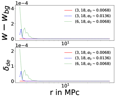
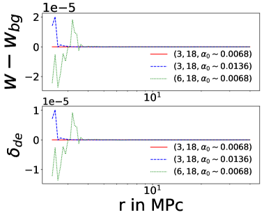
Figure 14: Effects of scale for small over dense case $(3,18)$. The fluctuations here are very weak and comparable to numerical noise. But they are suggestive of claims of made in article. Following figures clearly establish the claim that length scale of perturbations play a more important role.

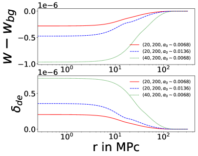
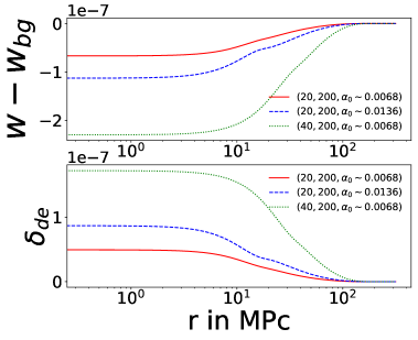
Figure 14(extra): Effects of scale and amplitude variation for under dense regions.

7 Effect of deviation in backgrounds

We had argued that perturbations in dark energy grow by a significant amount for models where $(1+w)$ is larger. This continues to hold with the corrected scaling, as can be seen in fig (16).

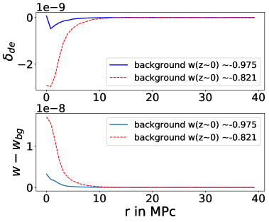
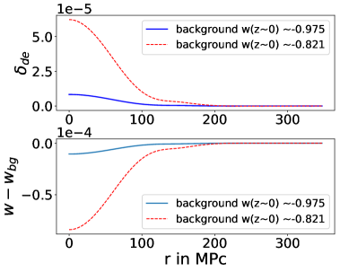
Figure 16: In this figure we study the impact of the equation of state parameter $w$ for the background on the growth of dark energy perturbations and the radial variation of the equation of state parameter. Here we show perturbation growth in two different background models for $V\propto\psi^{2}$. Curves are labeled by the present day values of $w$ for the background model. We see that the perturbations have a larger amplitude and $w$ has a larger variation for a larger $1+w_{0}$. The left panel here is for an over-density (OD1) and the right panel is for a void (UD5). We see that the effect is strongly pronounced for under density partly because of the larger scale of perturbation. The curves for over density are plotted for $z=1.5$, before virialisation of the innermost shells. Curves for UD5 are plotted at $z=0$.

8 Virialization condition for the field

In our work we considered three possibilities for dynamics of the scalar field dynamics in the virialized region. These are:

1. The scalar field can be evolved as a test field in the space-time determined by the frozen metric coefficients in the virialised region.

2. The scalar field can also be frozen in the virialised region, i.e., we put $\dot{\psi}=0=\ddot{\psi}$ in this region.

3. We put $\ddot{\psi}=0$ and freeze the value of $\dot{\psi}(r)$ inside the virial region.

We reported that “the differences between 3 approaches decrease rapidly beyond the turn around scale.” We find that while working with corrected scales, the second and 3rd approach show numerical instability. We use the stable and consistent approach, the first one, which was used in original article as well.

References

• [1] Manvendra Pratap Rajvanshi and J. S. Bagla. Nonlinear spherical perturbations in Quintessence Models of Dark Energy. JCAP, 06:018, 2018.