Valley current filtering and reversal by parallel side contacted armchair nanotubes

Abstract

The intertube conductance $G$ of the parallel side contacted armchair nanotubes is calculated by Landauer’s formula as a function of the Fermi level $E$. When the intertube difference in the dope strength is large enough, a resonant peak dominant over the others appears in the $E$-$G$ curve. The overlap length and the interlayer configuration do not influence the resonant energy. The intervalley transmission at the resonant peak works as a reverser and a filter of the valley current.

I introduction

Valleys – the $K$ and $K^{\prime}$ corner points in the two dimensional Brillouin zone – are crucial for distinguishing properties of the graphene (Gr) and the monolayer transition metal dichalcogenide (TMD).[1] An intervalley imbalance in the electron-hole recombination brings about the polarized light-emitting in the pn junction of TMD.[2] The valley current (VC) – an intervalley difference in current – does not necessarily accompany the charge current. [3] Owing to the high mobility, the Gr is more suitable for the VC technology than the TMD.[4] The Y-shaped bilayer Gr with oppositely charged top and back gates[5] separates the $K$ current from the $K^{\prime}$ current. The bubble structure[6] and line defects[7] in the single layer Gr transmit only one of the $K$ and $K^{\prime}$ currents. We call these systems VC filters (VCFs) because we obtain the single valley current from simultaneous incidence of the $K$ and $K^{\prime}$ currents. On the other hand, the Gr superlattice structure (GrS) [8] and partially overlapped Gr (po-Gr) [9] work as the VC reversers (VCR) that cause large intervalley transmission rates. Each of these systems, however, can be only one of the VCF and the VCR, while a structure that works both as the VCF and as the VCR is suitable for the integration of the VCF with the VCR in the device processing.

The carbon nanotube (NT) is similar to the Gr when the Gr satisfies the periodic boundary condition along the NT circumference. [10] Since the interlayer current is much smaller than the intralayer current in the multiwall NT and the multilayer Gr, one might consider that the interlayer current is irrelevant to the VCF and the VCR. In the parallel side contacted nanotube (ps-NT) and the telescoped NT (t-NT) schematically shown by Fig. 1, however, the interlayer current is equal to the intralayer current. [11, 12, 13, 14, 15] In addition, the overlap length can be controlled by mechanical motion of the attached piezo electrode. [16] When the NTs are armchair nanotubes (ANTs), the valley indexes are translated into the symmetry index $\sigma=+,-$ concerning the mirror plane on the ANT axis. In this case, the VCR producing the $\sigma$ VC is realized when $T_{\sigma,-\sigma}\simeq 1$ where $T_{\sigma,\sigma^{\prime}}$ denotes the transmission rate from valley $\sigma^{\prime}$ to valley $\sigma$. Since $T_{+,+}+T_{-,+}\leq 1$ and $T_{+,+}+T_{+,-}\leq 1$, a necessary condition for the VCR is (I) $T_{+,+}\simeq 0$. It is noteworthy that condition (I) is compatible with the condition of VCF, $T_{\sigma,\sigma}+T_{\sigma,-\sigma}\simeq 1\gg T_{-\sigma,\sigma}+T_{-\sigma,-\sigma}$.

According to the result of the t-ANT, condition (II) $|\varepsilon|\gg w_{+,+}$ is necessary for condition (I) where $\varepsilon$ is the intertube site energy difference of the tight binding model (TB) and $w_{+,+}$ denotes the interlayer Hamiltonian element corresponding to $T_{+,+}$.[12] Reflecting the relatively large interlayer area shown by the right panels of Fig. 1, the t-ANT has a much larger $w_{+,+}$ than the ps-ANT. In the range $|\varepsilon|\leq$ 0.5 eV, the t-ANT cannot be the VCR because the large $w_{+,+}$ conflicts with condition (II). Though the relatively small $w_{+,+}$ of the ps-ANT is favorable to achieving condition (II), the discussion about the nonzero $\varepsilon$ is limited to the t-ANT. In the experiment, the nonzero $\varepsilon$ can be induced by the encapsulated dopants, while it cannot be much larger than 0.5 eV.[17, 18, 19] This paper discusses whether the ps-ANT works as the VCR and the VCF with the realistic $\varepsilon$. Evidence of the VC other than nonlocal resistance ($R_{\rm NL}$) [20] is also a target of this paper as interpretation of $R_{\rm NL}$ in terms of the VC is still controversial. [21]

This paper is organized as follows. Section II defines the TB Hamiltonian. Section III shows the notation of the transmission rate for the discussion about the VCR and the VCF. In Sec. IV, the approximate formulas of the transmission rates are derived from the TB Hamiltonian. Section V defines the overlap integrals between the two ANTs to clarify the relationship between the transmission rate and the wave function . In Sec. VI, the origin of the VCR and the VCF is elucidated by the approximate formulas and the overlap integrals. A summary and a conclusion are presented in Sec. VII, where we comment on the experimental fingerprint of the VCR and the VCF.

II geometrical structure and TB Hamiltonian

Figure 2 (a) schematically shows that the ps-ANT is composed of partially overlapped two ANTs. We refer to the two ANTs as symbols $\downarrow$ and $\uparrow$. Symbols L (R) denotes the region in tube $\downarrow$ ($\uparrow$) excluding the overlap region D. Consider the honeycomb lattice $(\overline{y},\overline{z})$ on the $(y,z)$ plane where $\overline{y}=\frac{\sqrt{3}a}{2}(m-\frac{(-1)^{m}}{6}-\frac{(-1)^{j}}{2})$, $\overline{z}=\frac{a}{2}j$ with integers $j$, $m$ and the lattice constant $a=0.246$ nm. Converting $\overline{y}$ into the angles $\theta_{\downarrow}=\frac{\overline{y}}{r_{\downarrow}}$ and $\theta_{\uparrow}=\frac{\overline{y}}{r_{\uparrow}}-\frac{2\pi}{3n_{\uparrow}}+\theta_{\rm d}$ with the tube radii $r_{\xi}=\frac{\sqrt{3}a}{2\pi}n_{\xi}$ and a small rotation $|\theta_{\rm d}|<\pi/n_{\uparrow}$, we define the atomoc position $(x_{\xi},y_{\xi},z_{\xi})$ of tube $\xi(=\downarrow,\uparrow)$ as $y_{\xi}=r_{\xi}\sin\theta_{\xi}$, $x_{\downarrow}=r_{\downarrow}\cos\theta_{\downarrow}$, $x_{\uparrow}=r_{0}+r_{\downarrow}+r_{\uparrow}-r_{\uparrow}\cos\theta_{\uparrow}$ and $z_{\downarrow}=z_{\uparrow}-z_{\rm d}=\overline{z}$ with a small translation $|z_{\rm d}|<a/4$ and the interlayer distance $r_{0}=$ 0.31 nm. In tube $\xi$, $1\leq m\leq 2n_{\xi}$. Regions L, D and R correspond to the ranges $j\leq 0$, $1\leq j\leq N-2$ and $N-1\leq j$, respectively, where $N$ is an integer and the overlap length equals $\left(\frac{N}{2}-1\right)a-z_{\rm d}$. Figure 2 (b) shows the interlayer configuration in case $n_{\uparrow}=2n_{\downarrow}$ and $(\theta_{\rm d},z_{\rm d})=(0,0)$. The interlayer configuration is similar to the AB stacking when $z_{\rm d}=0$ and $\theta_{\rm d}=0,-2\pi/(3n_{\uparrow})$. [22]

According to the atomic position defined above, we define the TB Hamiltonian in the same way as Ref.[23]. The TB equations in region D are represented by

$$E\vec{c}_{j}^{\;(\rm D)}=\sum_{\Delta j=-1}^{1}H^{(j,\Delta j)}\vec{c}_{j+\Delta j}^{\;(\rm D)}$$ (1)

with the Hamiltonian matrix

$$H^{(j,\Delta j)} = \left(\begin{array}[]{cc}h_{\downarrow}^{(j,\Delta j)},&0\\ 0,&h_{\uparrow}^{(j,\Delta j)}\end{array}\right)$$ (7)

$$+\left(\begin{array}[]{cc}0,&W^{(j,\Delta j)}\\ \;^{t}W^{(j+\Delta j,-\Delta j)},&0\end{array}\right).$$

The first and second terms of Eq. (7) are intralayer $H_{\rm 0}^{(j,\Delta j)}$ and interlayer $V^{(j,\Delta j)}$ parts, respectively. The nearest neighbor elements of $H_{\rm 0}$ and the diagonal elements of $h_{\uparrow}^{(0,0)}$ equal $-t$ ($=-2.75$ eV) and $\varepsilon$, respectively, while the other elements of $H_{\rm 0}$ are zero.

The nonzero value of $\varepsilon$ can be realized when the two NTs have different doping strengths. For example, Fig. 1 schematically shows the pristine NT contacted with the iodine-encapsulated NT. [17] The iodine atoms become negatively charged and exert the repulsive potential to the host NT wall electron, while they have little influence on the other pristine NT. When a single iodine atom is encapsulated, the repulsive potential at a host NT’s carbon site increases as the carbon site approaches the iodine atom. On the other hand, when the iodine atoms are encapsulated densely and form the crystal, it is approximated by a positive constant $\varepsilon$ irrespective of the carbon site. We should also mention that the TB with the site energy shift is a standard tool for discussing the doping effect.[24]

The element of $W^{(j,\Delta j)}$ becomes nonzero only when the atomic distance $\overline{r}$ is shorter than the cut-off distance $r_{c}=$ 0.39 nm. The nonzero element is defined by $t_{1}\exp[(r_{1}-\overline{r})/r_{2}]\cos(\theta^{\downarrow}+\theta^{\uparrow})$ with parameters $t_{1}=$ 0.36 eV, $r_{1}=$ 0.334 nm and $r_{2}=$ 0.045 nm. The exact numerical calculation is performed in the same way as Ref. [14]. The same TB Hamiltonian is applied to both the exact and the approximate calculations.

III notation of the transmission rate

In Fig. 3 (a), (b), and (c), the rectangular area represents the scattering region D between regions L and R. The right and left going electrons are represented by $\rightarrow$ and $\leftarrow$, respectively. The Bloch wave function of region $\mu(=$ L,R) with unit flow is denoted by $\psi(\mu)$ with valley indexes $K,K^{\prime}$ and the propagation direction indexes $\rightarrow,\leftarrow$. The transmission rate from $\psi{\rm(L)}_{\flat,\rightarrow}$ to $\psi{\rm(R)}_{\sharp,\rightarrow}$ is denoted by $T_{\sharp,\flat}$ with valley indexes $\flat$ and $\sharp$. The conductance equals $T_{K,K}+T_{K^{\prime},K^{\prime}}+T_{K^{\prime},K}+T_{K,K^{\prime}}$ in unit of the quantum conductance $2e^{2}/h$ according to Landauer’s formula. [25] The wave functions of the isolated ANT are classified into the symmetric (+) and antisymmetric $(-)$ states with respect to the mirror plane parallel to the ANT axis. Thick solid lines in Fig. 3 (d) illustrate one to one correspondence between the symmetry indexes $+,-$ and the valley indexes $K,K^{\prime}$ concerning the $\rightarrow$ waves. Thus indexes $K,K^{\prime}$ are replaced by $+,-$ in the following sections. In this section, however, we keep the notation $K,K^{\prime}$ for comparison with other systems.

Figure 3 explains the transmission on condition (i) $T_{K^{\prime},K}=1$. In Fig. 3 (a), $\psi{\rm(L)}_{K,\rightarrow}$ is incident and perfectly transmitted to $\psi{\rm(R)}_{K^{\prime},\rightarrow}$. Since the time reversal operation converts $\psi{\rm(L)}_{K,\rightarrow}$ and $\psi{\rm(R)}_{K^{\prime},\rightarrow}$ into $\psi{(\rm L)}_{K^{\prime},\leftarrow}$ and $\psi{(\rm R)}_{K,\leftarrow}$, respectively, it also converts Fig. 3 (a) into Fig. 3 (b). In other words, the wave function of Fig. 3 (b) is the complex conjugate of that of Fig. 3 (a). It indicates that $T_{\sharp,\flat}$ coincides with the transmission rate from $\psi{\rm(R)}_{\sharp^{\prime},\leftarrow}$ to $\psi{\rm(L)}_{\flat^{\prime},\leftarrow}$ with the notation $(K^{\prime})^{\prime}=K$. The VC of region $\mu(=$ L,R) is defined as $J(\mu)_{v}=J(\mu)_{K}-J(\mu)_{K^{\prime}}$ where $J(\mu)_{\sharp}$ denotes the flow of electrons belonging to valley $\sharp(=K,K^{\prime})$ of region $\mu$. The VC is called ’pure’ especially when it is unaccompanied by the charge current. The pure VC can be generated and detected by the valley Hall effect and the inverse valley Hall effect.[26] The VC of region $\mu$ becomes pure on condition $J(\mu)_{K}+J(\mu)_{K^{\prime}}=0$.

Superposing Fig. 3 (a) on Fig. 3 (b), we find Fig. 3 (c) where $\psi{(\rm L)}_{K,\rightarrow}$ and $\psi{(\rm R)}_{K,\leftarrow}$ are simultaneously incident, and the positive pure VC of region L is converted into the negative pure VC of region R. It manifests the VCR for the positive pure $J{\rm(L)}_{v}$. In the same way, the ps-ANT works as the VCR for the negative pure $J{\rm(L)}_{v}$ on condition (ii) $T_{K,K^{\prime}}=1$. When conditions (i) $T_{K^{\prime},K}=1$ and (iii) $T_{K,K^{\prime}}=0$ are satisfied at the same time, on the other hand, the ps-ANT works as the VCF producing the valley polarized transmitted wave $\psi{(\rm R)}_{K^{\prime},\rightarrow}$ ($\psi{(\rm L)}_{K^{\prime},\leftarrow}$) from the valley unpolarized incidence $\psi{(\rm L)}_{K,\rightarrow}+\psi{(\rm L)}_{K^{\prime},\rightarrow}$ ( $\psi{(\rm R)}_{K,\leftarrow}+\psi{(\rm R)}_{K^{\prime},\leftarrow}$). Interchanging $K$ and $K^{\prime}$ in the discussion above, we can show the VCF producing $\psi{(\rm R)}_{K,\rightarrow}$ and $\psi{(\rm L)}_{K,\leftarrow}$.

IV Perturbative calculations

The energies with a wave number $k$ of the periodic system of which the unit cell is the same as region D are the eigen values of the matrix $H(k)=H_{\rm 0}(k)+V(k)$ with the notation

$$\spadesuit(k)=\left(\begin{array}[]{cc}\spadesuit^{(1,0)},&\diamondsuit\\ {}^{t}\diamondsuit^{*},&\spadesuit^{(2,0)}\end{array}\right)$$ (8)

where $\spadesuit=H,H_{\rm 0},V$ and $\diamondsuit=\spadesuit^{(1,1)}+e^{-ika}\spadesuit^{(1,-1)}$. The eigen values and eigen vectors of $H_{\rm 0}(k)$ are represented by

$$E_{\sigma,\xi}=\sigma t\left(2\cos\frac{ka}{2}-1\right)+\varepsilon\delta_{\xi,\uparrow}$$ (9)

and

$$\vec{b}_{\sigma,\xi}^{\;[0](\zeta)}=\left(\begin{array}[]{c}\vec{d}_{\sigma,\xi}^{\;[0]}\\ -\exp\left(i\frac{k}{2}a\right)\vec{d}_{\sigma,\xi}^{\;[0]}\end{array}\right),$$ (10)

respectively, where $\delta_{\uparrow,\uparrow}=1,\delta_{\downarrow,\uparrow}=0$,

$$\left(\begin{array}[]{cc}\vec{d}_{\sigma,\downarrow}^{[0]},&\vec{d}_{\sigma,\uparrow}^{[0]}\end{array}\right)=\sqrt{2}\left(\begin{array}[]{cc}\vec{g}_{\downarrow,\sigma},&0\\ 0,&\vec{g}_{\uparrow,\sigma}\end{array}\right)$$ (11)

and

$$\;{}^{t}\vec{g}_{\xi,\sigma}=\frac{1}{\sqrt{8n_{\xi}}}(1,\sigma,1,\sigma,\cdots,1,\sigma)$$ (12)

with $\sigma$ being + $(-)$ for the symmetric (antisymmetric) states. The $m$’th component of the Eq. (12) corresponds to integer $m$ of the first paragraph of Sec. II. The index $\zeta=\pm$ in Eq. (10) indicates that $k\simeq\zeta 2\pi/(3a)$. As is shown in Fig. 3 (d), $\zeta=\sigma$ ($\zeta=-\sigma$) for the $\leftarrow$ states ($\rightarrow$ states). We introduce the factor $(-1)$ in the lower part of Eq. (10) in order to limit the range of $k$ to the Brillouin zone $|k|<\pi/a$. The wave number $k$ satisfying Eq. (9) for the $\rightarrow$ states ($dE/dk>0$) is approximated by

$$k_{\sigma,\xi}=\frac{2}{a}\left(\frac{E-\varepsilon\delta_{\xi,\uparrow}}{\sqrt{3}t}-\sigma\frac{\pi}{3}\right)$$ (13)

when $k$ is close to $\pm 2\pi/(3a)$.

As we consider $V(k)$ to be the perturbation, Eqs. (9) and (10) represent the zeroth order states. Equation (12) is the same notation as Ref. [14]. The factor $\sqrt{2}$ in Eq. (11) is necessary for the orthonormality, $\;{}^{t}\!\left(\vec{b}_{\sigma,\xi}^{\;[0]}\right)^{*}\vec{b}_{\sigma^{\prime},\xi^{\prime}}^{\;[0]}=\delta_{\sigma,\sigma^{\prime}}\delta_{\xi,\xi^{\prime}}$. In contrast to the case of Ref. [14] , the linear bands $k_{\sigma,\uparrow}$ and $k_{\sigma,\downarrow}$ are not degenerate and the first order shift of the energy ${}^{t}(\vec{b}_{\sigma,\xi}^{[0]})^{*}V(k)\vec{b}_{\sigma,\xi}^{[0]}$ equals zero. The first order shift $\vec{b}^{[1]}$ in the wave function is represented by

$$\left(\begin{array}[]{c}{}^{t}\vec{b}_{+,\downarrow}^{[1],(\zeta)}\\ {}^{t}\vec{b}_{-,\downarrow}^{[1],(\zeta)}\end{array}\right)=2\left(\begin{array}[]{cc}\frac{-w_{+,+}^{(-\zeta)}}{\varepsilon},&\frac{w_{-,+}^{(-\zeta)}}{2E-\varepsilon}\\ \frac{w_{+,-}^{(-\zeta)}}{2E-\varepsilon},&\frac{-w_{-,-}^{(-\zeta)}}{\varepsilon}\end{array}\right)\left(\begin{array}[]{c}{}^{t}\vec{b}_{+,\uparrow}^{[0],(\zeta)}\\ {}^{t}\vec{b}_{-,\uparrow}^{[0],(\zeta)}\end{array}\right)$$ (14)

and

$$\left(\begin{array}[]{c}{}^{t}\vec{b}_{+,\uparrow}^{[1],(\zeta)}\\ {}^{t}\vec{b}_{-,\uparrow}^{[1],(\zeta)}\end{array}\right)=2\left(\begin{array}[]{cc}\frac{w_{+,+}^{(\zeta)}}{\varepsilon},&\frac{w_{+,-}^{(\zeta)}}{2E-\varepsilon}\\ \frac{w_{-,+}^{(\zeta)}}{2E-\varepsilon},&\frac{w_{-,-}^{(\zeta)}}{\varepsilon}\end{array}\right)\left(\begin{array}[]{c}{}^{t}\vec{b}_{+,\downarrow}^{[0],(\zeta)}\\ {}^{t}\vec{b}_{-,\downarrow}^{[0],(\zeta)}\end{array}\right)$$ (15)

where

$$w_{\sigma^{\prime},\sigma}^{(-)}\equiv\frac{1}{2}\;^{t}(\vec{b}_{\sigma^{\prime},\uparrow}^{[0],(+)})^{*}V\left(\frac{2\pi}{3a}\right)\vec{b}_{\sigma,\downarrow}^{[0],(+)}$$ (16)

and $w_{\sigma^{\prime},\sigma}^{(+)}=w_{\sigma^{\prime},\sigma}^{(-)*}$ in the same way as Ref. [14]. The explicit definition is

$$w_{\sigma^{\prime},\sigma}^{(\zeta)}=\sum_{j=1}^{2}\sum_{m=1}^{2n_{\downarrow}}\sum_{m^{\prime}=1}^{2n_{\uparrow}}\frac{(W^{(j,0)}-\widetilde{W}^{(j,1),(\zeta)})_{m,m^{\prime}}}{8\sigma^{m+1}(\sigma^{\prime})^{m^{\prime}+1}\sqrt{n_{\uparrow}n_{\downarrow}}}$$ (17)

where integers $m,m^{\prime}$ correspond to $m$ of the first paragraph of Sec. II and

$$\widetilde{W}^{(j,1)(\pm)}=e^{\pm i\frac{\pi}{3}}W^{(j,1)}+e^{\mp i\frac{\pi}{3}}W^{(j,-1)}.$$ (18)

Figure 4 is a schematic diagram of Eq. (13) in case $k\simeq 2\pi/(3a)$ and helps us to derive Eqs. (14) and (15). The dashed horizontal line indicates the Fermi level $E$ . The approximate eigenvectors $\vec{b}^{[0],(+)}+\vec{b}^{[1],(+)}$ up to the first order are calculated along the corresponding dotted vertical lines that indicate the Fermi wave numbers $-k_{+,\xi}$ and $k_{-,\xi}$ . The four closed symbols on the dashed horizontal line correspond to the unperturbed wave function $\vec{b}^{[0],(+)}$ at the energy $E$ while the first order shift $\vec{b}^{[1],(+)}$ is the linear combination of the states indicated by the open symbols. For example, the closed diamond corresponds to $\vec{b}^{[0],(+)}_{-,\downarrow}$ while the first order shift $\vec{b}^{[1],(+)}_{-,\downarrow}$ caused by $V(k_{-,\downarrow})$ is the superposition of the open diamonds. [27] Since $k_{-,\downarrow}\simeq 2\pi/(3a)$, the matrix elements of $V(k_{-,\downarrow})$ are approximated by those of $V(2\pi/(3a))$.

When we neglect modes other than the $\vec{b}^{[0]}+\vec{b}^{[1]}$ states defined by Eqs. (10), (14) and (15), the solution of Eq. (1) can be approximated by the repetition of the reduced vector $\vec{c}_{j}^{\;\prime(\rm D)}$ as $(\vec{c}_{j}^{\;\prime(\rm D)},\vec{c}_{j}^{\;\prime(\rm D)},\cdots,\vec{c}_{j}^{\;\prime(\rm D)})$. The neglect of the evanescent modes is justified when the overlap length is much larger than the NT radii, i.e., $N\gg n_{\downarrow},n_{\uparrow}$ because the decay length is about the NT radius at most. The reduced vector $\vec{c}_{j}^{\;\prime(\rm D)}$ is represented by

$$\vec{c}_{j}^{\;\prime(\rm D)}=\left(U_{\rm D}^{[0]}+U_{\rm D}^{[1]}\right)\sum_{s=\pm}\Xi^{s(j+1)}\vec{\gamma}_{s}^{(\rm D)}$$ (19)

The sign $s=+$ ($s=-$) corresponds to the $\rightarrow$ states ($\leftarrow$ states). The matrix $U_{\rm D}^{[n]}$ denotes the $n$’th order term for $\vec{c}_{-1}^{\;\prime({\rm D})}$,

$$U_{\rm D}^{[n]}=\left(\vec{d}^{\;\prime[n],(-)}_{+,\downarrow},\;\vec{d}^{\;\prime[n],(+)}_{-,\downarrow},\;\vec{d}^{\;\prime[n],(-)}_{+,\uparrow},\;\vec{d}^{\;\prime[n],(+)}_{-,\uparrow}\right)$$ (20)

where $\vec{d}^{\;\prime[0],(\zeta)}_{\sigma,\xi}$ is defined by Eq. (11) of which $\vec{g}_{\xi,\sigma}$ is replaced by $\vec{g}^{\;\prime}_{\xi,\sigma}=(1/\sqrt{8n_{\xi}})\;^{t}(1,\sigma)$. Replacing $\vec{b}_{\sigma,\xi}^{[n],(\zeta)}$ with $\vec{d}_{\sigma,\xi}^{\;\prime[n],(\zeta)}$ in Eqs. (14) and (15), we also obtain $\vec{d}^{\;\prime[1],(\zeta)}_{\sigma,\xi}$. Accordingly the index $\zeta$ in Eq. (20) is necessary only when $n=1$ as $\vec{d}^{\;\prime[0],(+)}=\vec{d}^{\;\prime[0],(-)}$ and $\vec{d}^{\;\prime[1],(+)}=\vec{d}^{\;\prime[1],(-)*}$. The phase factor matrix is derived from Eq. (13) as

$$\Xi\equiv\left(\begin{array}[]{cc}\beta_{1}\Omega,&0\\ 0,&\beta_{2}\Omega\end{array}\right)$$ (21)

where $\beta_{1}=e^{i\frac{E}{\sqrt{3}t}},\beta_{2}=e^{i\frac{E-\varepsilon}{\sqrt{3}t}}$ and

$$\Omega=\left(\begin{array}[]{cc}e^{i\frac{2}{3}\pi},&0\\ 0,&e^{-i\frac{2}{3}\pi}\end{array}\right)\;\;.$$ (22)

Replacing $U^{[1]}_{\rm D}$ with zero in Eq. (19), we obtain

$$\vec{c}_{j}^{\;\prime(\rm L)}=\frac{v_{0}}{\sqrt{n_{\downarrow}}}\\ \sum_{s=\pm}\left[\beta_{1}\Omega\right]^{s(j+1)}\vec{\gamma}_{s}^{(\rm L)}$$ (23)

for region L $(j\leq-1$),

$$\vec{c}_{j}^{\;\prime(\rm R)}=\frac{v_{0}}{\sqrt{n_{\uparrow}}}\\ \sum_{s=\pm}\left[\beta_{2}\Omega\right]^{s(j-N+1)}\vec{\gamma}_{s}^{(\rm R)}$$ (24)

for region R $(j\geq N-1)$, where

$$v_{0}=\frac{1}{2}\left(\begin{array}[]{cc}1,&1\\ 1,&-1\end{array}\right).$$ (25)

Equations (19), (23) and (24) enable us to transform the boundary conditions

$$\left(\begin{array}[]{cc}\vec{c}^{\;\prime(\rm D,\downarrow)}_{0},&\vec{c}^{\;\prime(\rm D,\uparrow)}_{N-2}\\ \vec{c}^{\;\prime(\rm D,\downarrow)}_{-1},&\vec{c}^{\;\prime(\rm D,\uparrow)}_{N-1}\\ \vec{c}^{\;\prime(\rm D,\uparrow)}_{-1},&\vec{c}^{\;\prime(\rm D,\downarrow)}_{N-1}\end{array}\right)=\left(\begin{array}[]{cc}\vec{c}^{\;\prime(\rm L)}_{0},&\vec{c}^{\;\prime(\rm R)}_{N-2}\\ \vec{c}^{\;\prime(\rm L)}_{-1},&\vec{c}^{\;\prime(\rm R)}_{N-1}\\ 0,&0\end{array}\right)$$ (32)

into formulas $(^{t}\!\vec{\gamma}^{\rm(D)}_{+},\;^{t}\!\vec{\gamma}^{\rm(L)}_{-})^{t}\!X_{\rm L}=-(^{t}\!\vec{\gamma}^{\rm(D)}_{-},\;^{t}\!\vec{\gamma}^{\rm(L)}_{+})^{t}\!X_{\rm L}^{*}$ and $(^{t}\!\vec{\gamma}^{\rm(D)}_{-}\Xi^{-N},\;^{t}\!\vec{\gamma}^{\rm(R)}_{+})^{t}\!X_{\rm R}=-(^{t}\!\vec{\gamma}^{\rm(D)}_{+}\Xi^{N},\;^{t}\!\vec{\gamma}^{\rm(R)}_{-})^{t}\!X_{\rm R}^{*}$ . Partitioning $U_{\rm D}^{[n]}$ as ${}^{t}U_{\rm D}^{[n]}=(^{t}U_{\rm L}^{[n]}/\sqrt{n_{\downarrow}},\;^{t}U_{\rm R}^{[n]}/\sqrt{n_{\uparrow}})$ , we derive the $n$’th order of $X_{\mu}$ matrix as

$$X_{\mu}^{[n]}=\left(\begin{array}[]{cc}U_{\mu}^{[n]}\Xi_{0},&-v_{0}\Omega^{*}\delta_{n,0}\\ U_{\mu}^{[n]},&-v_{0}\delta_{n,0}\\ U_{-\mu}^{[n]},&0\\ \end{array}\right)$$ (33)

with the notation $-$L =R and $-$R =L. In the derivation of Eq. (33), $E/t$ and $\varepsilon/t$ are neglected and $\Xi$ is replaced by

$$\Xi_{0}=\left(\begin{array}[]{cc}\Omega,&0\\ 0,&\Omega\end{array}\right).$$ (34)

The results of the perturbative calculation on the $S$ matrix $S_{\mu}=-X_{\mu}^{-1}X_{\mu}^{*}$ are

$$S_{\rm L} = \left(\begin{array}[]{ccc}0,&-F_{+}^{*},&{\bf 1}_{2}\\ -\;^{t}F_{+}^{*},&-{\bf 1}_{2},&-\;^{t}F_{+}\\ {\bf 1}_{2},&-F_{+}&0\\ \end{array}\right)$$ (38)

and

$$S_{\rm R} = \left(\begin{array}[]{ccc}-{\bf 1}_{2},&-F_{-},&-F_{-}^{*}\\ -\;^{t}F_{-},&0,&{\bf 1}_{2}\\ -\;^{t}F_{-}^{*},&{\bf 1}_{2},&0\\ \end{array}\right)$$ (42)

where

$$F_{\pm}=2\left(\begin{array}[]{cc}\frac{\mp w_{+,+}^{(\pm)}}{\varepsilon},&\frac{w_{-,+}^{(+)}}{2E-\varepsilon}\\ \frac{w_{+,-}^{(-)}}{2E-\varepsilon},&\frac{\mp w_{-,-}^{(\mp)}}{\varepsilon}\end{array}\right)\;\;.$$ (43)

Here ${\bf 1}_{n}$ denotes the unit matrix of $n$ dimension and the derivation of Eqs. (38) and (42) is shown in Appendix A. Equations (38) and (42) satisfy the time reversal symmetry $\;{}^{t}S_{\mu}=S_{\mu}$, while the unitarity $S_{\mu}^{*}S_{\mu}={\bf 1}_{6}$ holds up to the first order. Partitioning $S_{\mu}$ matrixes in Eqs. (38) and (42) as

$$S_{\mu}=\left(\begin{array}[]{cc}r_{\mu},&{}^{t}t_{\mu}\\ t_{\mu},&0\\ \end{array}\right),$$ (44)

The transmission rate block in the $S$ matrix of the double junction L-D-R corresponding to incidence from region L is represented by

$$t_{\rm RL}=t_{\rm R}\Xi^{N}\sum_{m=0}^{\infty}\;\left(r_{\rm L}\Xi^{N}r_{\rm R}\Xi^{N}\right)^{m}\;{}^{t}t_{\rm L}\;.$$ (45)

In the formula up to the first order, $t_{\rm RL}=(\beta_{1}\beta_{2}\Omega)^{N}t^{\prime}_{\rm RL}\Omega^{N}$ where

$$t^{\prime}_{\rm RL} = \;{}^{t}F^{*}_{+}(\beta_{1}\Omega)^{N}-\;^{t}F_{+}(\beta_{1}\Omega)^{-N}$$ (47)

$$+(\beta_{2}\Omega)^{N}\;{}^{t}F_{-}-(\beta_{2}\Omega)^{-N}\;{}^{t}F_{-}^{*}$$

As the first (second) row and column of Eq. (47) correspond to symmetric $+$ (antisymmetric $-$) channel, the transmission rate $|(t_{\rm RL})_{\sigma^{\prime},\sigma}|^{2}$ from $(\sigma,$L) to $(\sigma^{\prime},$R) is represented by $T_{\sigma^{\prime},\sigma}=16\frac{|w_{\sigma^{\prime},\sigma}|^{2}}{3t^{2}}Q_{\sigma^{\prime},\sigma}$ where

$$Q_{\sigma^{\prime},\sigma}=\left(\frac{\sin(\eta_{\sigma^{\prime},\sigma}^{(-\sigma\sigma^{\prime})}N)}{\eta_{\sigma^{\prime},\sigma}^{(-\sigma\sigma^{\prime})}}\cos(\eta^{(\sigma\sigma^{\prime})}_{\sigma^{\prime},\sigma}N-\phi_{\sigma^{\prime},\sigma})\right)^{2}$$ (48)

with the beat wave numbers $\eta_{\sigma^{\prime},\sigma}^{(\pm)}\equiv(k_{\sigma,\downarrow}\pm k_{\sigma^{\prime},\uparrow})a/4$ and the phase $\phi_{\sigma^{\prime},\sigma}$ of the parameter $w_{\sigma^{\prime},\sigma}^{(\sigma)}=|w_{\sigma^{\prime},\sigma}^{(\sigma)}|\exp(i\phi_{\sigma^{\prime},\sigma})$. The explicit formulas are

$$T_{\sigma,\sigma} = \frac{64|w_{\sigma,\sigma}|^{2}}{\varepsilon^{2}}\sin^{2}\left(\frac{\varepsilon N}{2\sqrt{3}t}\right)$$ (50)

$$\times\cos^{2}\left[\left(\frac{\widetilde{E}}{\sqrt{3}t}-\frac{\pi}{3}\sigma\right)N-\phi_{\sigma,\sigma}\right]$$

for the intravalley transmission ($\sigma\sigma^{\prime}=+$) and

$$T_{-\sigma,\sigma} = \frac{16|w_{-\sigma,\sigma}|^{2}}{\widetilde{E}^{2}}\sin^{2}\left(\frac{\widetilde{E}N}{\sqrt{3}t}\right)$$ (52)

$$\times\cos^{2}\left[\left(\frac{\varepsilon}{2\sqrt{3}t}-\frac{\pi}{3}\sigma\right)N-\phi_{-\sigma,\sigma}\right]$$

for the intervalley transmission ($\sigma\sigma^{\prime}=-$) with $\widetilde{E}\equiv E-\frac{\varepsilon}{2}$ being the energy measured from the cross point between the $E^{[0]}_{\downarrow}$ and $E^{[0]}_{\uparrow}$ bands. Equations (17) and (18) show that $|w_{\sigma^{\prime},\sigma}|$ is an even function of $z_{\rm d}$. Accordingly $\left.\frac{\partial|w_{-\sigma,\sigma}|}{\partial z_{\rm d}}\right|_{z_{\rm d}=0}=0$ and

$$\left.\frac{\partial T_{-\sigma,\sigma}}{\partial z_{\rm d}}\right|_{z_{\rm d}=0} = \left.\left(\frac{\partial\phi_{-\sigma,\sigma}}{\partial z_{\rm d}}\frac{\partial T_{-\sigma,\sigma}}{\partial\phi_{-\sigma,\sigma}}\right)\right|_{z_{\rm d}=0}$$ (53)

$$= \left.\frac{\partial\phi_{-\sigma,\sigma}}{\partial z_{\rm d}}\right|_{z_{\rm d}=0}C_{\sigma}\sin\left(\frac{\varepsilon N}{\sqrt{3}t}-\frac{2}{3}\pi\sigma N\right)$$ (54)

where $C_{\sigma}=16\frac{|w_{-\sigma,\sigma}|^{2}}{\widetilde{E}^{2}}\sin^{2}\left(\frac{\widetilde{E}N}{\sqrt{3}t}\right)$. We will refer to Eq. (54) in discussion about the dependence of $G$ on $z_{\rm d}$.

Equation (48) reproduces the analytical formulas of Ref. [14] only when $\sigma\sigma^{\prime}=-1$. An interpolation between Eq. (50) and the formula of Ref. [14] is

$$T_{\sigma,\sigma}=\frac{Y_{\sigma}}{Y_{\sigma}+\left[1-\frac{16|w_{\sigma,\sigma}|^{2}}{\Gamma_{\sigma}^{2}}\sin^{2}\left(\frac{\Gamma_{\sigma}N}{2\sqrt{3}t}\right)\right]^{2}}$$ (55)

where

$$Y_{\sigma} = \frac{64|w_{\sigma,\sigma}|^{2}}{\Gamma_{\sigma}^{2}}\sin^{2}\left(\frac{\Gamma_{\sigma}N}{2\sqrt{3}t}\right)\cos^{2}\left(\eta_{\sigma,\sigma}^{(+)}N-\phi_{\sigma,\sigma}\right)\;,$$ (56)

and

$$\Gamma_{\sigma}=\sqrt{\varepsilon^{2}+16|w_{\sigma,\sigma}|^{2}}\;\;.$$ (57)

Equations (50) and (56) are transformed into each other by the replacement $\varepsilon\leftrightarrow\Gamma_{\sigma}$. As $|w_{\sigma,\sigma}/\varepsilon|$ decreases, Eq. (55) approaches Eq. (50). On the contrary, Eq. (55) coincides with the formula of Ref. [14] when $\varepsilon=0$. In contrast to Eq. (50), Eq. (55) is always lower than unity as the transmission rate should be. We can derive Eq. (55) in the absence of the intervalley parameters $w_{-\sigma,\sigma}$ as is shown by Appendix B.

As is shown in Fig. 2 (a), the geometrical overlap length equals $(N-2)$ in the unit of $a/2$ while the overlap length in the analytical formulas (50), (52) and (55) seems $N$. The difference between the two kinds of the overlap lengths comes from the two margins at $j=-1,N-1$. For the relation between the overlap length and the integer $N$, we should refer to the TB model of $(N-1)$ atoms aligned at $z=ja/2$ ($j=0,1,2,\cdots,N-2)$ with a constant transfer integral $-t$. The eigen value $E$ and $j$’th component $c_{j}$ of the eigen vector $\vec{c}$ of the TB secular equation are represented by $E=-2\gamma\cos(k_{m}a/2)$ and $c_{j}=\sin(k_{m}a(j+1)/2)$, respectively, where $k_{m}=2\pi m/(Na)$ with the integers $m$ under the boundary conditions $c_{-1}=0$ and $c_{N-1}=0$. Here the system length in the formula of $k_{m}$ is $Na/2$ and less than the geometrical length $(N-2)a/2$.

V overlap integral analysis

To search Eqs. (52) and (56) for the characteristics of the wave function, the sc-ANT is mimicked by the double ladder (DL) in Fig. 5. The Hamiltonian of the DL is defined by Eq. (7) where $n_{\downarrow}=n_{\uparrow}=1$ and all the elements of $W$ are zero except that $W^{(1,0)}_{2,1}=W^{(2,0)}_{2,1}=t_{\bot}$. The intraladder transfer $-t$ and interladder transfer $t_{\bot}$ are indicated by the single line and the double line, respectively. The sites with the interladder transfer $t_{\bot}$ are depicted as double circles. Though the twisted DL in Fig. 5 (a) is topologically identical to the DL with staggered $t_{\bot}$ in Fig. 5 (b), the essential period $a/2$ is clarified in the former while the latter is in harmony with the real geometric structure. The secular equation $(E-H(k))\vec{b}=0$ of the DL is represented by

$$\left(\begin{array}[]{cccc}E,&-p,&0,&0\\ -p,&E,&-t_{\bot},&0\\ 0,&-t_{\bot},&E^{\prime},&-p\\ 0,&0,&-p,&E^{\prime}\end{array}\right)\vec{d}_{\rm D}=0$$ (58)

where $p=2t\cos(ka/2)-t$ and $E^{\prime}=E-\varepsilon$. The eigen vector is represented by

$$\;{}^{t}\vec{d}_{\rm D}=\left(1,\;q_{\rm r},\;q_{\uparrow}\left(\frac{E^{\prime}}{E}q_{\rm r},\;1\right)\right)$$ (59)

where

$$(q_{\rm r},q_{\uparrow})=\left(\frac{E}{p},\;\frac{E^{2}-p^{2}}{t_{\bot}E^{\prime}}\right)$$ (60)

$$p=\tau^{\prime}\sqrt{\widetilde{E}^{2}+\frac{\varepsilon^{2}}{4}+\tau\sqrt{(\varepsilon^{2}+t_{\bot}^{2})\widetilde{E}^{2}-\frac{\varepsilon^{2}t_{\bot}^{2}}{4}}}$$ (61)

$\tau=\pm 1$ and $\tau^{\prime}=\pm 1$. The relation between (59) and Fig. 5 is displayed in Fig. 6. The squared overlap integral between the unperturbed $\xi\;(=\downarrow,\uparrow)$ region and perturbed D region is calculated as

$$f_{\sigma,\xi}=\frac{\left|\;{}^{t}\vec{d}_{\rm D}\vec{d}^{\;\prime[0]*}_{\sigma,\xi}\right|^{2}}{\left|\vec{d}_{\rm D}\right|^{2}\left|\vec{d}^{\;\prime[0]}_{\sigma,\xi}\right|^{2}}$$ (62)

We speculate that the transmission rate $T_{\sigma^{\prime},\sigma}$ reflects the product of the squared overlap integrals defined by

$$I_{\sigma^{\prime},\sigma}=2\sum_{\tau^{\prime}=\pm}\sum_{\tau=\pm}f_{\sigma^{\prime},\uparrow}f_{\sigma,\downarrow}$$ (63)

The necessary conditions for the transmission rate $T_{\sigma^{\prime},\sigma}\leq 1$ and $T_{\sigma,\sigma}+T_{-\sigma,\sigma}\leq 1$ are shared by $I$ as proved in Appendix C.

VI Results and discussions

The system $n_{\downarrow}=5,n_{\uparrow}=10$ is considered as a typical example. The effect of $n_{\xi}$ will be discussed in the end of this section. Firstly we discuss the AB stacking configuration $(\theta_{\rm d},z_{\rm d})=(0,0)$. When $z_{\rm d}=0$, Eq. (17) is real and thus $\phi_{\sigma^{\prime},\sigma}=0,\pi$. The effect of nonzero $\theta_{\rm d}$, $z_{\rm d}$ will be shown latter. Figure 7 shows $T_{-,-}$ as a function of $N$ for the energy $E=0.15$ eV. It offers an archetypal example of the analysis of the $N$-$T_{\sigma,\sigma}$ curve by Eq. (55). The solid and dashed lines display the exact results and approximate formula (55), respectively, for five values of $\varepsilon=0,0.07,\cdots,0.28$ eV. Table I shows $w_{-,-}$. The residue $l$ of $N$ is defined by $l=N-3m$ with the integer $m$ under the condition $|l|\leq 1$. Since $|\eta_{\sigma^{\prime},\sigma}^{(\sigma\sigma^{\prime})}|\simeq\frac{\pi}{3}$ in Eq. (48), the beat wave number $\eta_{\sigma^{\prime},\sigma}^{(\sigma\sigma^{\prime})}$ causes the rapid oscillation with the period $\Delta N=3$ . In order to make the slow oscillation of the other beat wave number $\eta_{\sigma^{\prime},\sigma}^{(-\sigma\sigma^{\prime})}$ noticeable, we fix the residue $l$ to 0, 1 and $-1$ in the upper, middle and lower panels, respectively, in Fig. 7. Overall agreement between the dashed and solid lines is fairly good. For the quantitative comparison, the nodes of the dashed lines are listed in Table II. The zero points of Eq. (55) are represented by $N=(6m-3-2l)\lambda_{E}/6$ and $N=m\lambda_{\Gamma}$ with $\lambda_{E}=\pi\sqrt{3}t/\widetilde{E}$, $\lambda_{\Gamma}=2\pi\sqrt{3}t/\Gamma$ and integers $m$. Owing to the agreement between the solid and dashed lines, the nodes of the solid lines in Fig. 7 can be also identified as those in Table II. When $\varepsilon=0.14$ eV, all the lines approach zero at $N=200$ corresponding to the node $\lambda_{\Gamma}=201$. When $\varepsilon=0.14$ eV and $l=-1$, the nodes $\lambda_{\Gamma}=201$ and $5\lambda_{E}/6=156$ are close to each other, thus $T_{-,-}$ is remarkably suppressed between the nodes $156<N<201$ in the bottommost panel. The topmost panel also shows the similar suppression between the nodes $\lambda_{\Gamma}=139$ and $\lambda_{E}/2=166$ when $\varepsilon=$ 0.21 eV. We cannot discern the nodes $N=16.6,21.7$ and 31.2 in the middle panel, whereas they cause the apparent depletion of $T_{-,-}$ in the region $N<30$ compared to the other panels. The approximate formula (55) reproduces the suppression of the exact $T_{-,-}$ by the increase of $\varepsilon$. The suppressed $T_{-,-}$ of $\varepsilon=0.21,0.28$ eV in the middle panel is magnified in the inset. The lines with circles correspond to case $\varepsilon=0.21$ eV. Though Eq. (55) overestimates (underestimates) $T_{-,-}$ when $\varepsilon=0.21$ eV and $N>50$ ($\varepsilon=0.28$ eV and $N>100$), the dashed and solid lines share the important characteristic that they are remarkably smaller than those for $\varepsilon=0.14,0.07,0$ eV. In the dashed lines of the inset, we can identify the nodes $\lambda_{\Gamma}=139,105$, $\frac{\lambda_{E}}{6}=55.4$. Although Eq. (55) is verified when $\varepsilon=0$ or $|\varepsilon|\gg 4|w_{\sigma,\sigma}|$, agreement between the solid and dashed lines with $\varepsilon=0.07$ eV manifests the effectiveness of Eq. (55) in the interpolated region $|\varepsilon|\simeq 4|w_{\sigma,\sigma}|$. The same result is found in $T_{+,+}$ (not shown in Figures).

Equation (55) is effective not only in the ps-ANTs but also in the t-ANTs. In this paragraph, we concentrate our discussion into the intravalley transmission rate $T_{\sigma,\sigma}$ of the t-ANTs. In Ref. [12] , Author considered the averaged transmission rate $\overline{T}(N)=\frac{1}{3}(T(N-2)+T(N)+T(N+2))$ in order to remove the rapid oscillations and derived

$$\overline{T}_{\sigma,\sigma}{\rm(Ref.\;12)}=16\frac{|w_{\sigma,\sigma}|^{2}}{\Gamma^{2}_{\sigma}}\sin^{2}\left(\frac{\Gamma_{\sigma}N}{2\sqrt{3}t}\right)$$ (64)

When $|\varepsilon|\gg 8|w_{\sigma,\sigma}|$, on the other hand, $Y_{\sigma}\ll 1$ and Eq. (55) is close to $Y_{\sigma}$. In that case, the averaged transmission rate $\overline{Y}_{\sigma}$ with the approximation $\cos^{2}(\eta^{(+)}_{\sigma,\sigma}N-\phi_{\sigma,\sigma})\simeq\cos^{2}(\pi N/3)$ is twice as large as Eq. (64). In this way, the multiple reflection ignored in Ref. [12] doubles $\overline{T}_{\sigma,\sigma}$ when $\overline{T}_{\sigma,\sigma}\ll 1$. In the results displayed in Ref. [12] , we are aware that Eq. (64) is only half of the exact averaged transmission rate when $T_{\sigma,\sigma}\ll 1$. The factor two in the formula $\overline{Y}_{\sigma}\simeq\overline{T}_{\sigma,\sigma}{\rm(Ref.\;12})\times 2$ has corrected this disagreement.[28]

In order to satisfy the condition $T_{-\sigma,\sigma}\gg T_{\sigma,\sigma}$, $|\varepsilon|$ has to be large enough to suppress $T_{\sigma,\sigma}$. In the following, we set $\varepsilon$ at 0.3 eV. It is comparable to the experimentally evaluated value 0.6 eV.[17] Under the conditions $|\varepsilon|,|\widetilde{E}|\ll\sqrt{3}t$ and $z_{\rm d}=0$, Eqs. (50) and (52) approximately satisfy the relations

$$T_{\sigma^{\prime},\sigma}(\widetilde{E},N)=T_{\sigma^{\prime},\sigma}(-\widetilde{E},N_{E})$$ (65)

and

$$T_{\sigma^{\prime},\sigma}(\widetilde{E},N)|w_{-\sigma^{\prime},-\sigma}|^{2}=T_{-\sigma^{\prime},-\sigma}(\widetilde{E},N_{w})|w_{\sigma^{\prime},\sigma}|^{2}$$ (66)

where $N_{E}$ and $N_{w}$ are related to $N=3m+l$ as $(N_{E},N_{w})=(3m-\sigma^{\prime}\sigma l,3m-l)$ with integers $m$ and residues $l=0,\pm 1$. The origin of Eq. (65) can be traced back to the beat wave number $\eta^{(+)}_{\sigma^{\prime},\sigma}$. Equation (55) also satisfies Eq. (65) under the same conditions, while increase of $|w_{\sigma,\sigma}|$ weakens effectiveness of Eq. (66) for Eq. (55). In the following, however, we discuss the results for $\varepsilon=0.3$ eV being much larger than $4|w_{\sigma,\sigma}|$. In that case, difference between Eqs. (55) and (50) is so small that Eq. (55) also approximately satisfies Eq. (66).

Equations (52) and (55) in case $l=1$ are exhibited in Fig. 8 with the range $N=4,7,10,\cdots,100$ and $|E|<0.3$ eV. The intravalley (55) reaches a local maximum when $N\simeq\lambda_{\Gamma}(m-\frac{1}{2})$ and $E=\frac{\varepsilon}{2}+\pi\sqrt{3}t\left(m^{\prime}+\frac{\sigma}{3}l\right)/N$ with integers $m$ and $m^{\prime}$. As for the local maximums i $\sim$ iv in Fig. 8, $m^{\prime}=0,-1$ and $N\simeq\lambda_{\Gamma}/2$. On the other hand, v and vi denote the local maximums of the intervalley formula (52) that appear when $E=\varepsilon/2$ and $x\tan(x-\frac{\pi}{3}\sigma l)=1$ with the notation $x=\varepsilon N/(2\sqrt{3}t)$. Figure 9 displays the exact numerical data corresponding to Fig. 8. We are satisfied by the agreement between Fig. 8 and Fig. 9 when we remember that there is no fitting parameter in Eqs. (52) and (55). As the parameters $w_{\sigma^{\prime},\sigma}$ shown in Table I are determined uniquely by Eq. (17) with the interlayer transfer integrals $W$, we cannot modify $w_{\sigma^{\prime},\sigma}$ in order to improve the agreement. For the quantitative comparison between Fig. 8 and Fig. 9, numerical values of $(N,E,T)$ at the local maximums are shown in Table III. Difference between Fig. 8 and Fig. 9 in Table III is satisfactorily small, though the positive (negative) $E$ tends to suppress (enhance) the exact $T$ in comparison to Eqs. (52) and (55). Figure 10 is the same exact calculations as in Fig. 9 except the residue $l=-1$. The analytical results corresponding to Fig. 10 can be found in Fig. 8 with the transformation (66). According to the transformation (66), $T_{-\sigma^{\prime},-\sigma}$ of Fig. 8 is multiplied by $(w_{\sigma^{\prime},\sigma}/w_{-\sigma^{\prime},-\sigma})^{2}$ and is shown in the rightmost column of Table III. It coincides well with $T_{\sigma^{\prime},\sigma}$ of Fig. 10. Since $E($ii$)+E($iv$)=\varepsilon$, Eq. (65) can be applied to ii and iv. It follows that $T($ ii, Fig. 9) $\simeq$ $T($ iv, Fig. 10) and $T($ ii, Fig. 10) $\simeq$ $T($ iv, Fig. 9). Figures 11 and 12 are the approximate and exact calculations as in Fig. 8 and Fig. 9, respectively, in case $l=0$. When $l=0$, $N_{w}=N$ and $T_{\mp,-}=T_{\pm,+}(w_{\mp,-}/w_{\pm,+})^{2}$ in Eq. (66). It follows that the surfaces $(N,E,T_{\mp,-})$ have the same shape as $(N,E,T_{\pm,+})$ in Eqs. (52) and (55) , thus we show only $T_{\pm,+}$ in Fig. 11. Figure 12 also shows that $T_{\pm,+}$ and $T_{\mp,-}$ are similar in shape. Table IV shows a comparison between Figs. 11 and 12 in the same way as Table III. There are eight local maximums labeled by $\bullet$i $\sim$ $\bullet$iv, ($\bullet=\triangle,\Box$) in Fig. 12. In comparison to $\bullet$iii, the peak $\bullet$iv is very low and cannot be visible in Figs. 11 and 12. The local maximums $\triangle$i $\sim$ $\triangle$iv in Fig. 12 are reproduced properly in Fig. 11. The heights of $\triangle$ peaks of Fig. 11 are transformed into those of the $\Box$ peaks by Eq. (66) in the rightmost column of Table IV. Overall, the transformed values appropriately reproduce the $\Box$ peaks in Fig. 12, except for the overestimation of the $\Box$iii peak height.

$w_{+,+}$	$w_{-,-}$	$w_{-,+}$	$w_{+,-}$
10.78	$-12.62$	$-9.372$	$12.62$

TABLE I.: The parameter $w_{\sigma^{\prime},\sigma}$ [meV] in case $(n_{\downarrow},n_{\uparrow})=(5,10)$ and $(\theta_{\rm d},z_{\rm d})=(0,0)$.

$\varepsilon$ [eV]	0	0.07	0.14	0.21	0.28
$\frac{1}{2}\lambda_{E},\;\frac{3}{2}\lambda_{E}$	49.9, 150	65.1, 195	93.5, *	166, *	*, *
$\frac{1}{6}\lambda_{E},\;\frac{7}{6}\lambda_{E}$	16.6, 116	21.7, 152	31.2, *	55.4, *	*, *
$\frac{5}{6}\lambda_{E},\;\frac{11}{6}\lambda_{E}$	83.1,  183	108, *	156, *	*, *	*, *
$\lambda_{\Gamma}$	*	*	201	139	105

TABLE II.: The nodes of dashed lines in Fig. 7 . They are $\frac{1}{2}\lambda_{E},\;\frac{3}{2}\lambda_{E}$ $(l=0)$, $\frac{1}{6}\lambda_{E},\;\frac{7}{6}\lambda_{E}$ $(l=1)$, $\frac{5}{6}\lambda_{E},\;\frac{11}{6}\lambda_{E}$ $(l=-1)$ and $\lambda_{\Gamma}$. The nodes outside the region $0<N<200$ are indicated by * except $\lambda_{\Gamma}=201$.

	Fig. 8 $(l=1)$			Fig. 9 $(l=1)$			Fig. 10 $(l=-1)$
	$N$	$E$	$T$	$N$	$E$	$T$	$N$	$E$	$T$
i	49	$-54$	0.078	49	$-65$	0.088	47	$-62$	0.111	0.107
ii	49	252	0.078	49	248	0.058	47	262	0.091	0.107
iii	49	$-257$	0.104	43	$-297$	0.121	47	$-289$	0.104	0.076
iv	49	48	0.104	46	43	0.099	47	37	0.071	0.076
v	52	150	0.116	49	147	0.122	50	145	0.165	0.210
vi	79	150	0.598	76	153	0.418	77	150	0.305	0.330

TABLE III.: The local maximums in Figs. 8, 9 and 10. The unit of $E$ is meV. According to the transformation (66), $T_{-\sigma^{\prime},-\sigma}$ of Fig. 8 is multiplied by $(w_{\sigma^{\prime},\sigma}/w_{-\sigma^{\prime},-\sigma})^{2}$ and is compared to $T_{\sigma^{\prime},\sigma}$ of Fig. 10 in the rightmost column.

	Fig. 11 $(\bullet=\triangle)$			Fig. 12 $(\bullet=\triangle)$			Fig. 12 $(\bullet=\Box)$
	$N$	$E$	$T$	$N$	$E$	$T$	$N$	$E$	$T$
$\bullet$i	48	$-162$	0.078	48	$-173$	0.096	48	$-153$	$0.117$	0.107
$\bullet$ii	48	$150$	0.078	51	145	0.067	51	152	0.098	0.107
$\bullet$iii	108	150	0.675	105	151	0.520	105	151	0.683	1.224
$\bullet$iv	27	150	0.020	27	129	0.025	24	165	0.027	0.036

TABLE IV.: The local maximums of Figs. 11 and 12. The unit of $E$ is meV. According to the transformation (66), $T_{-\sigma^{\prime},-\sigma}$ of Fig. 11 is multiplied by $(w_{\sigma^{\prime},\sigma}/w_{-\sigma^{\prime},-\sigma})^{2}$ and is compared to $T_{\sigma^{\prime},\sigma}$ of Fig. 12 in the rightmost column.

The exact dispersion relation near the valley $k=\frac{2\pi}{3a}$ is displayed in Fig. 13 for the discrete energies with the interval 0.002 eV. In contrast to the approximate dispersion relation in Fig. 4, the energy gap appears near the cross point at $E=\varepsilon/2=0.15$ eV, or equivalently, $\widetilde{E}=0$. In the energy gap, the evanescent waves replace the propagating waves. Accordingly, the phase factor $e^{ika}$ is replaced by $e^{(ik\pm\kappa)a}$ in the exact calculation. The decay factors $e^{-\kappa a}$ are displayed by the horizontal axes with the vertical axis $E$ in the inset of Fig. 13. As has been reported by Ref. [15], the decay length $1/\kappa$ is considerably long. It suggests the persistence of the propagating characteristic that enables Eqs. (52) and (55) remain effective in the gap. Figures 14 and 15 show (a) $T_{\sigma,\sigma}$ and (b) $T_{-\sigma,\sigma}$ as a function of $N$ at the center of the gap $E=\varepsilon/2$. Black and grey lines correspond to $\sigma=+$ and $\sigma=-$, respectively. As for the residue $l$, $l=1$ in Fig. 14 and $l=0$ in Fig. 15. We can distinguish the exact results from the approximate ones in the same way as Fig. 7. Because Eq. (52) exceeds unity for the large $N$, the dashed lines of the intervalley $T_{-\sigma,\sigma}$ are limited to the small $N$. The insets show the magnification of the intervalley $T_{-\sigma,\sigma}$. The local maximums $\triangle$iv and $\Box$iv in Figs. 11 and 12 can be visible. Agreement between the solid and dashed lines is satisfying in the range $N<50$. In a wider range of $N$, the solid and dashed lines do not necessarily coincide with each other, while the periods of the solid lines excellently coincide with that of the dashed lines $2\sqrt{3}t\pi/\varepsilon\simeq 100$. Though the height ratio between the neighboring peaks in the solid line fluctuates, it approaches $e^{-\kappa 100a}\simeq(0.992)^{100}=0.45$ as $N$ increases. It comes from the decay characteristic of the gap state.

Figure 16 displays the product of the squared overlap integrals (63) for the four values of $\varepsilon=$ 0, 0.05, 0.1, 0.15 eV. Applying Eq. (17), we obtain $w_{\sigma^{\prime},\sigma}=\sigma^{\prime}t_{\bot}/4$. As Table I shows $w_{\sigma^{\prime},\sigma}\simeq 0.01\sigma^{\prime}$ eV, $t_{\bot}$ is set to 0.04 eV. The black and gray (red online) lines indicate the intervalley $I_{-\sigma,\sigma}$ and intravalley $I_{\sigma,\sigma}$, respectively. They reproduce the qualitative dependence of $T_{\sigma^{\prime},\sigma}$ on $\varepsilon$ and $E$. The asymptotic formulas of $I_{\sigma^{\prime},\sigma}$ are shown by Table V in case (a) $|\widetilde{E}|\ll|\varepsilon|,|t_{\bot}|$ and case (b) $|\widetilde{E}|\gg|\varepsilon|,|t_{\bot}|$ with the parameter $\alpha=\varepsilon/t_{\bot}$. Since $|w|=|t_{\bot}|/4$, the factors $64|w|^{2}/\Gamma^{2}$ and $16|w|^{2}/\widetilde{E}^{2}$ in Eqs. (56) and (52) are translated to $4/(1+\alpha^{2})$ and $|t_{\bot}/\widetilde{E}|^{2}$, respectively. Multiplying them by $1/4$, we get the terms $\delta_{\sigma,\sigma^{\prime}}/(1+\alpha^{2})$ and $\frac{1}{4}\delta_{\sigma,-\sigma^{\prime}}|t_{\bot}/\widetilde{E}|^{2}$ in Table V. Here we can speculate that the factor $1/4$ comes from the average $\lim_{N\rightarrow\infty}\frac{1}{N}\sum_{j=1}^{N}\sin^{2}(a^{\prime}j)\cos^{2}(b^{\prime}j-\phi)=1/4$ with the constants $a^{\prime},b^{\prime}$ and $\phi$. Figure 6 gives us an illuminating insight into Table V as follows. Firstly, we discuss case (a) where Eq. (60) is approximated by $q_{\rm r}=\tau^{\prime}\alpha/\sqrt{\alpha^{2}+2i\tau|\alpha|}$ and $q_{\uparrow}=\pm i$. The left-to-right amplitude ratio is 1 to $q_{\rm r}$ in ladder $\downarrow$, while 1 to $-q_{\rm r}$ in ladder $\uparrow$ because $E^{\prime}/E=-1$. As the ladders $\downarrow$ and $\uparrow$ are nearly opposite in the symmetry in this way, $I_{-\sigma,\sigma}>I_{\sigma,\sigma}$ in case (a). When $\alpha$ approaches zero, however, $q_{\rm r}$ also approaches zero. The limit is the average of a symmetric state and an antisymmetric one. Accordingly $I_{-\sigma,\sigma}=I_{\sigma,\sigma}$ when $\varepsilon=\widetilde{E}=0$. Next Let us discuss case (b) where $q_{\rm r}\simeq\tau^{\prime}\frac{E}{|E|}=\pm 1,q_{\uparrow}\simeq\alpha-\tau\frac{E}{|E|}\sqrt{1+\alpha^{2}}$. The two ladders have almost the same left-to-right amplitude ratio since $E^{\prime}/E\simeq 1$. Therefore $I_{-\sigma,\sigma}$ is much less than $I_{\sigma,\sigma}$. The small nonzero $I_{-\sigma,\sigma}$ being inversely proportional to $\widetilde{E}^{2}$ originates from the slight difference of $|q_{\rm r}|$ from 1 as is explained by Appendix D. In order to understand the term $\delta_{\sigma^{\prime},\sigma}/(1+\alpha^{2})$ in Table V, we should refer to the parameter $|q_{\uparrow}|$ that represents the interladder localization. As $\alpha$ approaches zero, $|q_{\uparrow}|$ tends to 1. It leads to the extended state between the two ladders and the large $I_{\sigma,\sigma}$. When $|\alpha|\gg 1$, on the other hand, $|q_{\uparrow}|$ is close to $(2|\alpha|)^{\pm 1}$. It causes the localized state at the single ladder and the small $I_{\sigma,\sigma}$ .

	(a) $|\widetilde{E}|\ll|\varepsilon|,|t_{\bot}|$	(b) $|\widetilde{E}|\gg|\varepsilon|,|t_{\bot}|$
arbitrary $\alpha$	$\frac{1}{2}-\frac{\sigma\sigma^{\prime}|\alpha|}{|\alpha|+\sqrt{\alpha^{2}+1}}$	$\frac{\delta_{\sigma,\sigma^{\prime}}}{1+\alpha^{2}}+\delta_{\sigma,-\sigma^{\prime}}\frac{2\alpha^{2}+1}{8\alpha^{2}+8}t_{\bot}^{2}\widetilde{E}^{\;-2}$
$\alpha=0$	$\frac{1}{2}$	$\delta_{\sigma,\sigma^{\prime}}+\delta_{\sigma,-\sigma^{\prime}}\frac{1}{8}t_{\bot}^{2}\widetilde{E}^{\;-2}$
$\alpha=\infty$	$\delta_{\sigma,-\sigma^{\prime}}$	$\delta_{\sigma,-\sigma^{\prime}}\frac{1}{4}t_{\bot}^{2}\widetilde{E}^{\;-2}$

TABLE V.: Asymptotic formulas of Eq. (63) with the parameter $\alpha=\varepsilon/t_{\bot}$

As examples of the influence of $\theta_{\rm d}$ and $z_{\rm d}$, Fig. 17 shows the conductance $G=\sum_{\sigma,\sigma^{\prime}}T_{\sigma^{\prime},\sigma}$ in the unit of $2e^{2}/h$ as a function of the energy $E$ in case $(\theta_{\rm d},z_{\rm d})=(0,\pm a/20),(-\pi/50,0),(\pi/30,0)$, $N=$ 101, 102, 103. The black and gray lines correspond to $\theta_{\rm d}=0$ and $z_{\rm d}=0$, respectively. The dashed (solid) lines show the approximate (exact) results. Though $w_{\sigma^{\prime}\sigma}$ becomes different from that of Table I, the condition $|w_{\sigma^{\prime},\sigma}|\ll|\varepsilon|$ remains valid. Thus the resonant peaks of the intervalley terms $T_{+,-},T_{-,+}$ remain dominant. We can see that the center of the peak, $E=\varepsilon/2$, is insensitive to $N$, $\theta_{\rm d}$ and $z_{\rm d}$. When the $\theta_{\rm d}=-\pi/30$, the mirror planes of the two tubes coincide with each other, and thus $w_{+,-}=w_{-,+}=0$. It explains why the conductance of $\theta_{\rm d}=-\pi/50$ is remarkably smaller than the other $\theta_{\rm d}$. Except the case $\theta_{\rm d}=-\pi/50$ where the agreement between the solid and dashed lines is fairy good, the dashed lines show overestimated values of $G$. Nevertheless the resonant intervalley peak survives in all the solid lines. Equation (54) enables us to approximate the difference $\Delta G\equiv G\left(\frac{a}{20}\right)-G\left(\frac{-a}{20}\right)$ for the black dashed lines of Fig. 17 as $\frac{a}{10}\sum_{\sigma}C_{\sigma}\sin\left(-\frac{2}{3}\pi\sigma N\right)\frac{\partial\phi_{-\sigma,\sigma}}{\partial z_{\rm d}}$ where $\varepsilon N/(\sqrt{3}t)\simeq 2\pi$. Since $C_{+}\simeq C_{-}>0$ and $\frac{\partial\phi_{+,-}}{\partial z_{\rm d}}-\frac{\partial\phi_{-,+}}{\partial z_{\rm d}}>0$, $\Delta G$ has the same sign as $\sin(2\pi N/3)$, i. e., $\Delta G(N=101)<0$, $\Delta G(102)\simeq 0$, and $\Delta G(103)>0$. This result is consistent with the solid black lines indicating that the effect of $z_{\rm d}$ is appropriately included by Eq. (52).

Some peaks in Fig. 14 (b) and Fig. 15 (b) approximately satisfy the conditions of the VCR and the VCF discussed in Sec. III. The peak indicated by $\triangleright$ ($\triangleleft$) in Fig. 14 (b) works not only as the VCR for the positive (neative) pure $J{\rm(L)}_{v}$ but also as the VCF producing the $\psi{(\rm R)}_{K^{\prime},\rightarrow}$ ( $\psi{(\rm R)}_{K,\rightarrow}$ ). On the other hand, the peak indicated by $\circ$ in Fig. 15 (b) approximately satisfies both (i) $T_{K^{\prime},K}=1$ and (ii) $T_{K,K^{\prime}}=1$ , indicating the VCR irrespective of the sign of the pure $J{(\rm L)}_{v}$, while it does not work as the VCF. Since the GrS and the po-Gr of Refs. [8, 9] must obey the condition $T_{\sigma^{\prime},\sigma}=T_{-\sigma^{\prime},-\sigma}$ that conflicts with the condition of the VCF, they cannot be the VCF. Contrary to it, Eq. (66) explicitly shows that $T_{\sigma^{\prime},\sigma}\neq T_{-\sigma^{\prime},-\sigma}$ for the ps-ANT. Note that the time reversal symmetry is no guarantee of the condition $T_{\sigma^{\prime},\sigma}=T_{-\sigma^{\prime},-\sigma}$.

The nonzero terms in Eq. (17) are limited to the sites $\theta_{j,m}\simeq 0$ in the ps-ANTs, whereas they spread over the all $m$ in the t-ANTs. It follows that $w_{+,+}$ of the t-ANTs is comparable to $t_{1}(=0.36$ eV) being much larger than $w_{+,+}$ of the ps-ANTs. As it is difficult to make $|\varepsilon|$ much larger than $t_{1}$, the ps-ANT is more suitable than the t-ANT for the condition $|\varepsilon|\gg w_{+,+}$. The perturbative calculation is effective on condition that $|E|,|\varepsilon|,|w_{\sigma^{\prime},\sigma}|\ll t$. The condition $|w_{\sigma^{\prime},\sigma}|\ll t$ always holds. The other conditions $|E|,|\varepsilon|\ll t$ are also satisfied except when the applied gate voltage and the doping strength are extremely high. Author has confirmed the approximate formulas (52) and (55) reproduce the exact results irrespective of the choice of $n_{\xi}$ (not shown in Figures). The effect of $n_{\xi}$ on Eqs. (52) and (55) can be derived from Eq. (17) that is the explicit relation between $w_{\sigma^{\prime},\sigma}$ and the interlayer Hamiltonian $W$. Though various atoms and molecules can be encapsulated, some of them might be unsuitable for the VCR and VCF. When europium and potassium atoms are encapsulated, for example, the current via the metal nanowire [18] and the nearly free electron states [19] might hide the VCR and the VCF. For more detailed discussions, the first principle calculation (FP) is desirable. To apply Eq. (16) to the FP, we only have to replace the wave function $\vec{b}$ and the interlayer Hamiltonian elements $W$ with those of the FP. [13]

VII summary and conclusion

The interlayer transmission rates of the ps-ANTs have been calculated by the $\pi$ orbital TB with the intertube site energy difference $\varepsilon$. The valley channels can be interpreted as the symmetric $(+)$ and antisymmetric $(-)$ channels concerning the plane including the tube axis. Considering the interlayer transfer integral to be the perturbation, we have derived the approximate analytical formulas (50) and (52) that is determined by the electron energy $E$, the integer overlap length $N$ and the interlayer Hamiltonian element $w_{\sigma^{\prime},\sigma}$ between $\sigma^{\prime}$ and $\sigma$ channels. The geometrical overlap length equals $(N-2)\frac{a}{2}-z_{\rm d}$ with the lattice constant $a=$ 0.246 nm and the small translation $|z_{\rm d}|<\frac{a}{4}$. Equation (17) enables us to transform the TB interlayer transfer integrals into $w_{\sigma^{\prime},\sigma}$ without a fitting parameter. The effect of $z_{\rm d}$ is included by $w_{\sigma^{\prime},\sigma}$.

In comparison to Ref.[14] , the nonzero $\varepsilon$ requires only a slight difference in the numerical code of the exact calculation. The perturbative calculations, however, have to be performed in a qualitatively different way since the nonzero $\varepsilon$ lifts the degeneracy of the unperturbed system. As $|\varepsilon|$ deceases, the system approaches the degenerate case and the perturbation theory for the nondegenerate case becomes ineffective. It is the reason why Eq. (50) with zero $\varepsilon$ does not reproduce the formula in Ref.[14] . Therefore it is not a trivial result that Eq. (52) with zero $\varepsilon$ is identical with the formula in Ref. [14]. Equation (55) is an interpolation between the degenerate case $(\varepsilon=0$, Ref. [14] ) and the nondegenerate case Eq. (50). The effective range of Eqs. (52) and (55) with respect to $E$ and $N$ is satisfyingly large. Tables III and IV are the guides for the quantitative comparison between the exact results and the approximate analytical formulas. They afford an archetypal example of the effectiveness of the analytical formulas.

The product of the squared overlap integrals (63) has a close relation to the wave function and explains the averaged transmission rate $\frac{1}{N}\sum_{j=1}^{N}T(N)$ with sufficiently large $N$. Figure 6 and Eq. (59) clearly indicate that the VCR $T_{-\sigma,\sigma}\simeq 1\gg T_{\sigma,\sigma}$ occurs when $|q_{\uparrow}|\simeq|q_{\rm r}|\simeq 1$ and $E^{\prime}/E\simeq-1$, i.e., on condition that $\widetilde{E}=0$ and $|\varepsilon|\gg|t_{\bot}|(\simeq 4|w|)$. In order to interpret the dependence on $N$, however, Eq. (63) is ineffective while Eqs. (52) and (55) are necessary. The peak at $E=\varepsilon/2$ in the $E$-$T_{-\sigma,\sigma}$ curve survives the change of the interlayer configuration $(\theta_{\rm d},z_{\rm d})$ if the two mirror planes are not very close to each other. At the peak energy $E=\varepsilon/2$, the oscillation of the exact $N$-$T_{-\sigma,\sigma}$ curve grows into about unit first, then decays exponentially. The factor of the corresponding analytical formula $N^{2}\cos^{2}\left(\frac{\varepsilon N}{2\sqrt{3}t}\pm\frac{\pi}{3}N\right)$ might be the origin of the former growing oscillation.

The ps-ANT works both as the VCR and as the VCF, for example, peaks indicated by $\triangleleft,\triangleright,\circ$ in Figs. 14 (b) and 15 (b). The resonant peak in the $E$-$G$ curve corresponding to the VCR and the VCF has two distinguishing characteristics not found in other double junction systems. Firstly the peak energy $E=\varepsilon/2$ is not affected by the overlap length. In the experiment, the mechanical motion of the piezo electrode attached to each ANT enables us to modulate the overlap length with other parameters unchanged. Secondly, it is evident from Eq. (52) that the peak at $E=\varepsilon/2$ is dominant over the other peaks. In contrast, multiple peaks have similar heights in the usual $E$-$G$ curve. These characteristics are fingerprints of the VCR and the VCF.

A Derivation of Eqs. (38) and (42)

The explicit formulas of Eq. (33) are

$$X^{[0]}_{\rm L}=V_{0}\left(\begin{array}[]{ccc}\Omega,&0,&-\Omega^{*}\\ {\bf 1}_{2},&0,&-{\bf 1}_{2}\\ 0,&{\bf 1}_{2}&0\\ \end{array}\right),$$ (A1)

$$X^{[1]}_{\rm L} = V_{0}\left(\begin{array}[]{ccc}0,&F_{-}\Omega&0\\ 0,&F_{-},&0\\ \;^{t}F_{+},&0&0\\ \end{array}\right),$$ (A5)

$$X^{[0]}_{\rm R}=V_{0}\left(\begin{array}[]{ccc}0,&\Omega&-\Omega^{*}\\ 0,&{\bf 1}_{2},&-{\bf 1}_{2}\\ {\bf 1}_{2},&0,&0\\ \end{array}\right),$$ (A6)

$$X^{[1]}_{\rm R} = V_{0}\left(\begin{array}[]{ccc}\;^{t}F_{+}^{*}\Omega,&0,&0\\ \;^{t}F_{+}^{*},&0,&0\\ 0,&F_{-}^{*},&0\\ \end{array}\right)$$ (A10)

with the notation

$$V_{0}=\left(\begin{array}[]{ccc}v_{0},&0,&0\\ 0,&v_{0},&0\\ 0,&0,&v_{0}\\ \end{array}\right)$$ (A11)

Inverse matrixes of Eqs.(A1) and (A6 ) are represented by

$$\left(X^{[0]}_{\rm L}\right)^{-1}=\frac{-i}{\sqrt{3}}\left(\begin{array}[]{ccc}\sigma_{z},&-\Omega^{*}\sigma_{z},&0\\ 0,&0,&i\sqrt{3}\\ \sigma_{z}\par,&-\Omega\sigma_{z},&0\\ \end{array}\right)V_{0}^{-1}$$ (A12)

$$\left(X^{[0]}_{\rm R}\right)^{-1}=\frac{-i}{\sqrt{3}}\left(\begin{array}[]{ccc}0,&0,&i\sqrt{3}\\ \sigma_{z},&-\Omega^{*}\sigma_{z},&0\\ \sigma_{z}\par,&-\Omega\sigma_{z},&0\\ \end{array}\right)V_{0}^{-1}$$ (A13)

with the Pauli matrix $\sigma_{z}$. The following is the perturbation series of $S_{\mu}=-X_{\mu}^{-1}X_{\mu}^{*}$ up to the first order.

$$S_{\mu} = -\left(X_{\mu}^{[0]}\right)^{-1}X_{\mu}^{[0]*}$$ (A15)

$$+\left(X_{\mu}^{[0]}\right)^{-1}\left[X_{\mu}^{[1]}\left(X_{\mu}^{[0]}\right)^{-1}X_{\mu}^{[0]*}-X_{\mu}^{[1]*}\right]$$

From these equations, we obtain Eqs. (38) and (42).

B derivation of Eq. (55) in the absence of the intervalley scattering

When we neglect the intervalley parameters $2w_{\pm,\mp}$, the eigen value equation $H(k)\vec{b}=E\vec{b}$ for symmetry $\sigma$ becomes

$$\left(\begin{array}[]{cc}E-E_{\sigma,\downarrow},&-2w_{\sigma,\sigma}\\ -2w_{\sigma,\sigma}^{*},&E-E_{\sigma,\downarrow}-\varepsilon\end{array}\right)\left(\begin{array}[]{c}d_{\sigma,\downarrow}^{\prime}\\ d_{\sigma,\uparrow}^{\prime}\end{array}\right)=\left(\begin{array}[]{c}0\\ 0\end{array}\right)$$ (B1)

where $w_{\sigma,\sigma}=w_{\sigma,\sigma}^{(\sigma)}$ and $E_{\sigma,\downarrow}$ is determined by Eq. (9). We derive the dispersion relation

$$E=\sigma t\left[2\cos\left(\frac{k_{m}}{2}a\right)-1\right]+\frac{\varepsilon+(-1)^{m}\Gamma_{\sigma}}{2}$$ (B2)

from Eq. (B1) where $m=1,2$. Whereas the first order shift of the energy is zero in Sec. IV, Eq. (B2) depends on the interlayer element $2w_{\sigma,\sigma}$. Here neglect of the intervalley $w_{\mp,\pm}$ is the tradeoff for the nonzero energy shift caused by the intravalley $w_{\sigma,\sigma}$. The wave function of region D is represented by

$$\left(\begin{array}[]{c}c_{j,\downarrow}^{\;\prime(\rm D)}\\ c_{j,\uparrow}^{\;\prime(\rm D)}\end{array}\right)=\sum_{s=\pm}\left(\begin{array}[]{cc}c_{\sigma}^{(s)},&-s_{\sigma}^{(s)}\\ s_{\sigma}^{(-s)},&c_{\sigma}^{(-s)}\end{array}\right)\Xi_{\sigma}^{s(j+1)}\vec{\gamma}_{s}^{\;(\rm D)}$$ (B3)

where

$$(c_{\sigma}^{(\pm)},\;s_{\sigma}^{(\pm)})=e^{\pm i\frac{\phi_{\sigma,\sigma}}{2}}\left(\sqrt{\frac{\varepsilon+\Gamma_{\sigma}}{2\Gamma_{\sigma}}},\;-\sqrt{\frac{-\varepsilon+\Gamma_{\sigma}}{2\Gamma_{\sigma}}}\right)$$ (B4)

and $(\Xi_{\sigma})_{m,m^{\prime}}=-\delta_{m,m^{\prime}}\exp(ik_{m}a/2)$. In the following, we use abbreviations $c_{\sigma}=c_{\sigma}^{(+)}$ and $s_{\sigma}=s_{\sigma}^{(+)}$. When $k_{m}\simeq-2\pi\sigma/(3a)$, $\Xi_{\sigma}$ is approximated by

$$\Xi_{\sigma}=-\exp(i\eta_{\sigma,\sigma}^{(+)})\left(\begin{array}[]{cc}e^{i\frac{\Gamma_{\sigma}}{2\sqrt{3}t}},&0\\ 0,&e^{-i\frac{\Gamma_{\sigma}}{2\sqrt{3}t}}\end{array}\right)\;\;.$$ (B5)

By the replacement $U_{\mu}^{[n]}\rightarrow(c_{\sigma},-s_{\sigma}),$ $U_{-\mu}^{[n]}\rightarrow(s^{*}_{\sigma},c^{*}_{\sigma})$, $v_{0}\rightarrow 1$, $\Omega^{*}\delta_{n,0}\rightarrow\exp(-2i\sigma\pi/3)$ and $\Xi_{0}\rightarrow\Xi_{\sigma}\rightarrow\exp(2i\sigma\pi/3)$ in Eq. (33), we can obtain

$$X_{\sigma,\rm L}=\left(\begin{array}[]{ccc}c_{\sigma}e^{i\sigma\frac{2}{3}\pi},&-s_{\sigma}e^{i\sigma\frac{2}{3}\pi},&-e^{-i\sigma\frac{2}{3}\pi}\\ c_{\sigma},&-s_{\sigma},&-1\\ s_{\sigma}^{*},&c_{\sigma}^{*},&0\end{array}\right)$$ (B6)

where $\widetilde{E}/t$ and $\Gamma_{\sigma}/t$ are approximated by zero. We can easily calculate $S_{\sigma,\rm L}=-X_{\sigma,\rm L}^{-1}X_{\sigma,\rm L}^{*}$ as

$$S_{\sigma,\rm L}=\left(\begin{array}[]{ccc}-s_{\sigma}^{2},&-c_{\sigma}s_{\sigma},&c_{\sigma}^{*}\\ -c_{\sigma}s_{\sigma},&-c_{\sigma}^{2},&-s_{\sigma}^{*}\\ c_{\sigma}^{*},&-s_{\sigma}^{*},&0\end{array}\right)$$ (B7)

Replacing $c_{\sigma}$ and $s_{\sigma}$ by $s_{\sigma}$ and $-c_{\sigma}$, respectively, we also obtain $X_{\sigma,\rm R}$ and $S_{\sigma,\rm R}$. Using Eqs. (B5) , (B7) and $S_{\sigma,{\rm R}}$ in Eq. (45), we can derive Eq. (55).

C The Upper limit of $I_{\sigma^{\prime},\sigma}$ and $I_{\sigma,\sigma}+I_{-\sigma,\sigma}$

With the notations

$$(a_{1},a_{2},a_{3})=\left(\frac{E}{\bar{p}_{\tau}},\;\frac{E^{2}-\bar{p}_{\tau}^{2}}{t_{\bot}\bar{p}_{\tau}},\;\frac{E^{2}-\bar{p}_{\tau}^{2}}{t_{\bot}E^{\prime}}\right)$$ (C1)

and

$$\bar{p}_{\tau}=\sqrt{\widetilde{E}^{2}+\frac{\varepsilon^{2}}{4}+\tau\sqrt{(\varepsilon^{2}+t_{\bot}^{2})\widetilde{E}^{2}-\frac{\varepsilon^{2}t_{\bot}^{2}}{4}}}\;,$$ (C2)

Eq. (59) is represented by

$$\;{}^{t}\vec{d}_{\rm D}=(1,\;\tau^{\prime}a_{1},\;\tau^{\prime}a_{2},\;a_{3})\;.$$ (C3)

Note that $a_{1},a_{2}$ and $a_{3}$ do not depend on $\tau^{\prime}$. Equation (63) is represented by

$$I_{\sigma^{\prime},\sigma} = \frac{1}{2}\sum_{\tau^{\prime}=\pm}\sum_{\tau=\pm}\frac{\left|1+\sigma\tau^{\prime}a_{1}\right|^{2}\left|a_{2}+\sigma^{\prime}\tau^{\prime}a_{3}\right|^{2}}{\left|1+|a_{1}|^{2}+|a_{3}|^{2}+|a_{4}|^{2}\right|^{2}}$$ (C4)

$$= Q^{(1)}_{+}+Q^{(1)}_{-}+\sigma\sigma^{\prime}(Q^{(2)}_{+}+Q^{(2)}_{-})$$ (C5)

where

$$Q^{(1)}_{\tau}=\frac{a_{4}a_{5}}{(a_{4}+a_{5})^{2}}\leq\frac{1}{4}$$ (C6)

$$Q^{(2)}_{\tau}=\frac{(a_{1}+a_{1}^{*})(a_{2}a_{3}^{*}+a_{3}a_{2}^{*})}{(a_{4}+a_{5})^{2}}$$ (C7)

with the notations $a_{4}=1+|a_{1}|^{2},\;a_{5}=|a_{2}|^{2}+|a_{3}|^{2}$. Formulas (C5) and (C6) enable us to derive

$$I_{\sigma,\sigma}+I_{-\sigma,\sigma}=2(Q^{(1)}_{+}+Q^{(1)}_{-})\leq 1\;.$$ (C8)

Since $I_{\sigma,\sigma}\geq 0$ and $I_{-\sigma,\sigma}\geq 0$, Eq. (C8) indicates that $I_{\sigma,\sigma}\leq 1$ and $I_{-\sigma,\sigma}\leq 1$.

D The asymptotic formula of $I_{-\sigma,\sigma}$ when $|\widetilde{E}|\rightarrow\infty$

Since

$$\lim_{|\widetilde{E}|\rightarrow\infty}\frac{q_{\uparrow}^{2}}{2\left|\vec{d}_{\rm D}\right|^{4}}=\frac{1}{32(\alpha^{2}+1)}$$ (D1)

with the parameter $\alpha=\varepsilon/t_{\bot}$,

$$\lim_{|\widetilde{E}|\rightarrow\infty}I_{-\sigma,\sigma}=\lim_{|\widetilde{E}|\rightarrow\infty}\sum_{\tau=\pm}\sum_{\tau^{\prime}=\pm}\frac{Q^{(3)}}{32(\alpha^{2}+1)}$$ (D2)

where

$$Q^{(3)} = (1+\sigma q_{\rm r})^{2}\left(1-\sigma q_{\rm r}\frac{E-\varepsilon}{E}\right)^{2}$$ (D3)

$$= \left(1+\frac{\frac{\varepsilon^{2}}{4}-\widetilde{E}^{2}}{\bar{p}_{\tau}^{2}}+\frac{\sigma\tau^{\prime}\varepsilon}{\bar{p}_{\tau}}\right)^{2}$$ (D4)

with $\bar{p}_{\tau}$ defined by Eq. (C2). Applying Eq. (D4) to Eq. (D2), we obtain

$$\lim_{|\widetilde{E}|\rightarrow\infty}I_{-\sigma,\sigma}=\frac{2\alpha^{2}+1}{8(\alpha^{2}+1)}\left(\frac{t_{\bot}}{\widetilde{E}}\right)^{2}$$ (D5)

since

$$\lim_{|\widetilde{E}|\rightarrow\infty}\frac{1}{\bar{p}_{\tau}}=\frac{1}{|\widetilde{E}|}$$ (D6)

and

$$\lim_{|\widetilde{E}|\rightarrow\infty}\frac{\widetilde{E}^{2}}{\bar{p}_{\tau}^{2}}=1-\tau\frac{\sqrt{\varepsilon^{2}+t_{\bot}^{2}}}{|\widetilde{E}|}\;\;.$$ (D7)

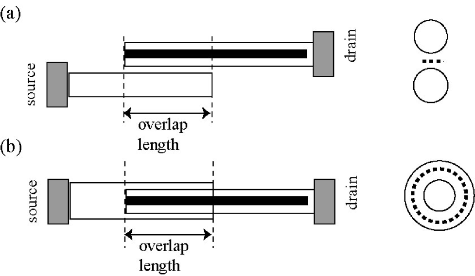
FIG. 1.: Schematic diagrams of (a) the parallel side contacted nanotube (ps-NT) and (b) the telescoped NT (t-NT). The two NTs overlap partially. The right panels are the cross-sectional views of the overlap regions where the dotted lines indicate the interlayer regions. The radius difference of the t-NT is close to the interlayer distance of the graphite. The gray rectangular are the source and drain electrodes. The black bar within the NT represents densely encapsulated iodine atoms.

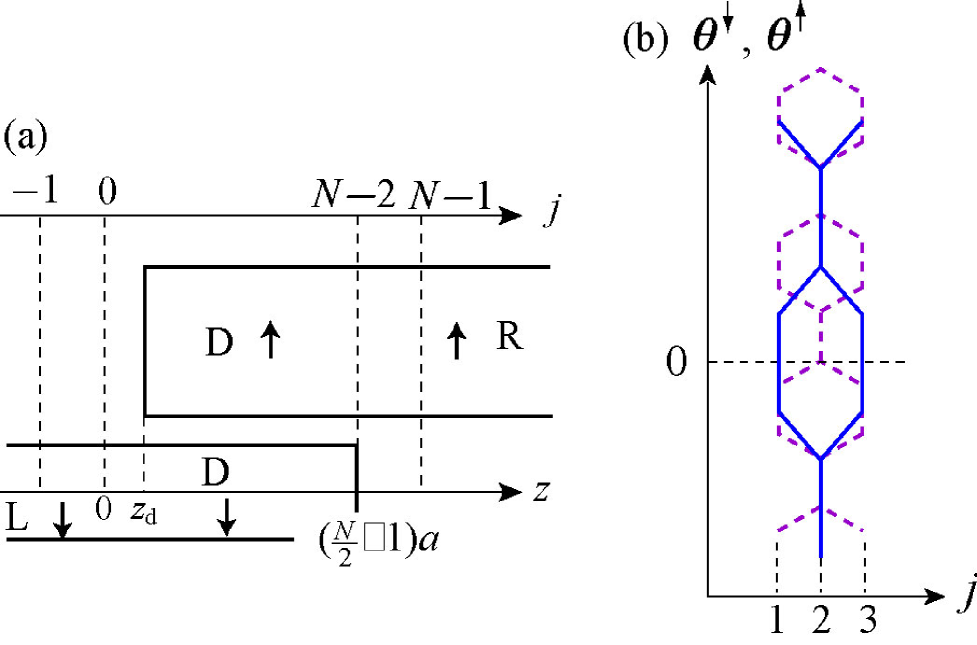
FIG. 2.: (a) The spatial configuration of the ps-ANTs (b) The interlayer configuration when $(\theta_{\rm d},z_{\rm d})=(0,0)$ and $n_{\uparrow}=2n_{\downarrow}$.

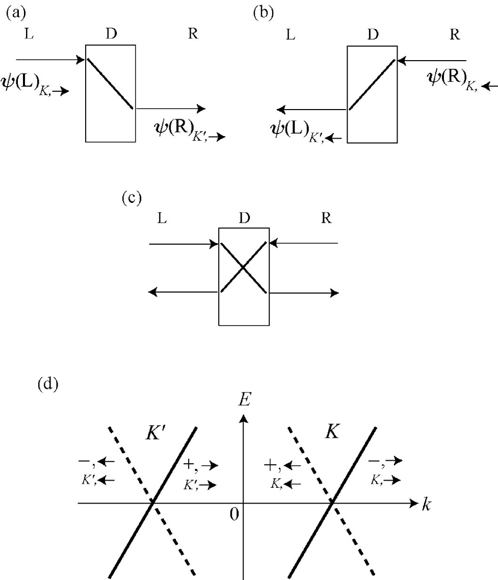
FIG. 3.: (a), (b) , (c) Transmission on condition (i) $T_{K^{\prime},K}=1$ where $\psi{(\mu)}_{\sharp,\rightarrow}$ ( $\psi{(\mu)}_{\sharp,\leftarrow}$) denotes the Bloch wave function of region $\mu(=$ L,R) and of valley $\sharp(=K,K^{\prime})$ with positive (negative) $\frac{dE}{dk}$. (a) $\psi{\rm(L)}_{K,\rightarrow}$ is incident. (b) $\psi{\rm(R)}_{K,\leftarrow}$ is incident. (c) $\psi{\rm(L)}_{K,\rightarrow}$ and $\psi{\rm(R)}_{K,\leftarrow}$ are incident at the same time. (d) The dispersion relation near the valleys $K$ and $K^{\prime}$. The right $(\rightarrow)$ and left $(\leftarrow)$ going waves correspond to the solid and dotted dispersion lines, respectively.

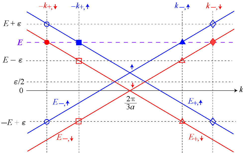
FIG. 4.: The schematic diagram of Eq. (13) in case $k\simeq 2\pi/(3a)$.

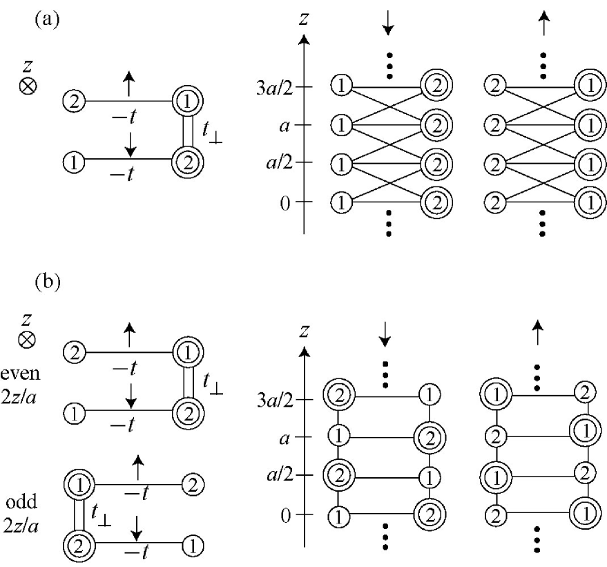
FIG. 5.: Two diagrams of the Hamiltonian. (a) twisted double ladder with the periodic interladder transfer integral $t_{\bot}$. (b) double ladder with staggered $t_{\bot}$.

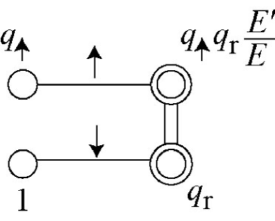
FIG. 6.: Relation between Fig. 5 and Eq. (59).

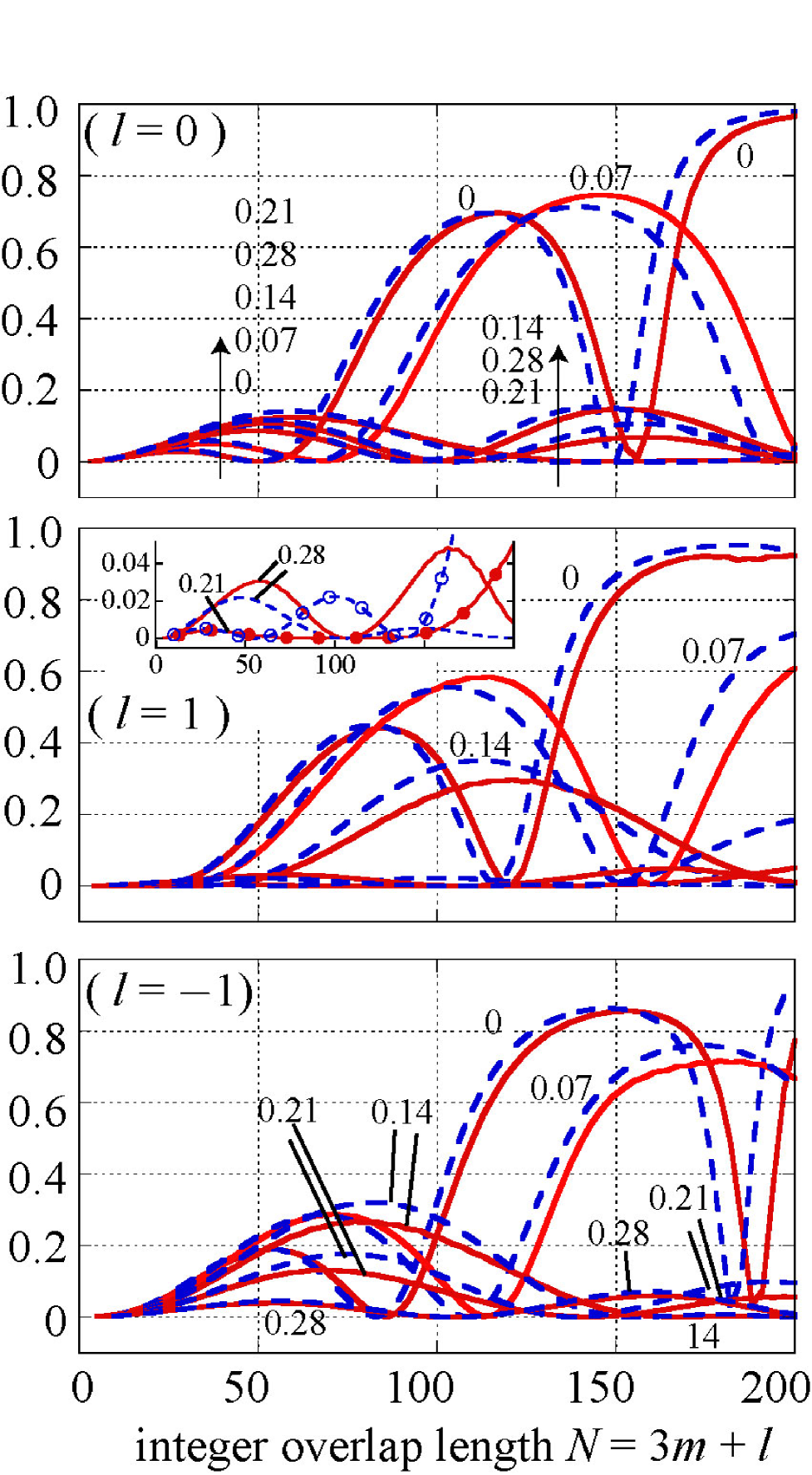
FIG. 7.: $T_{-,-}$ as a function of the integer overlap length $N$ for the energy $E=0.15$ eV and for the site energy difference $\varepsilon=$ 0, 0.07,,0.14, 0.21 and 0.28 eV. The solid and dashed lines display the exact results and Eq. (55), respectively. In each panel, $N=3m+l$ of which the integer $m$ is varied while the residue $l$ is fixed to 0, 1 and $-1$. The nodes of the dashed lines are listed in Table II.

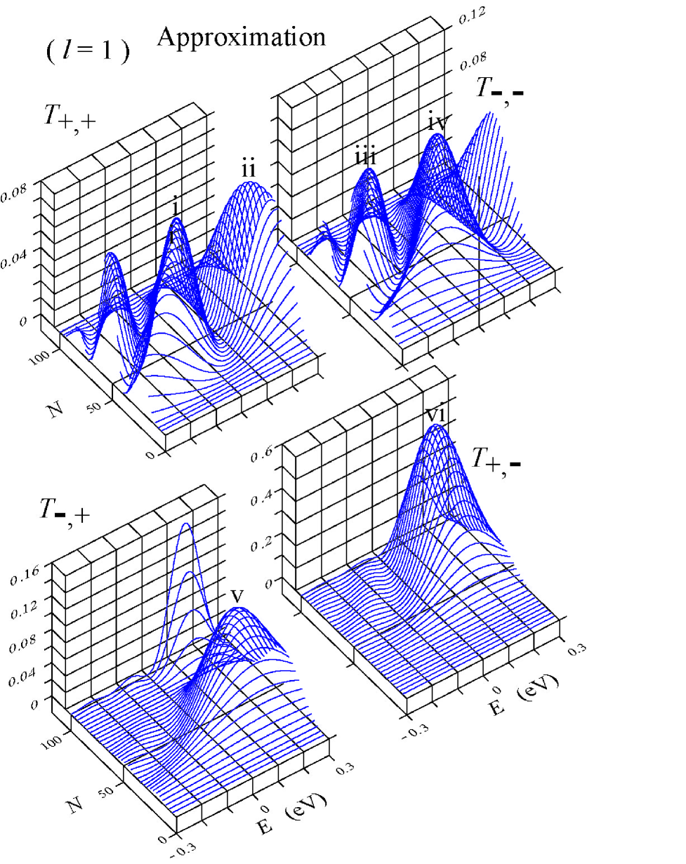
FIG. 8.: Three dimensional view of Eqs. (52) and (55) in case $l=1$, $\varepsilon=$ 0.3 eV, $\theta_{\rm d}=0$ and $z_{\rm d}=0$.

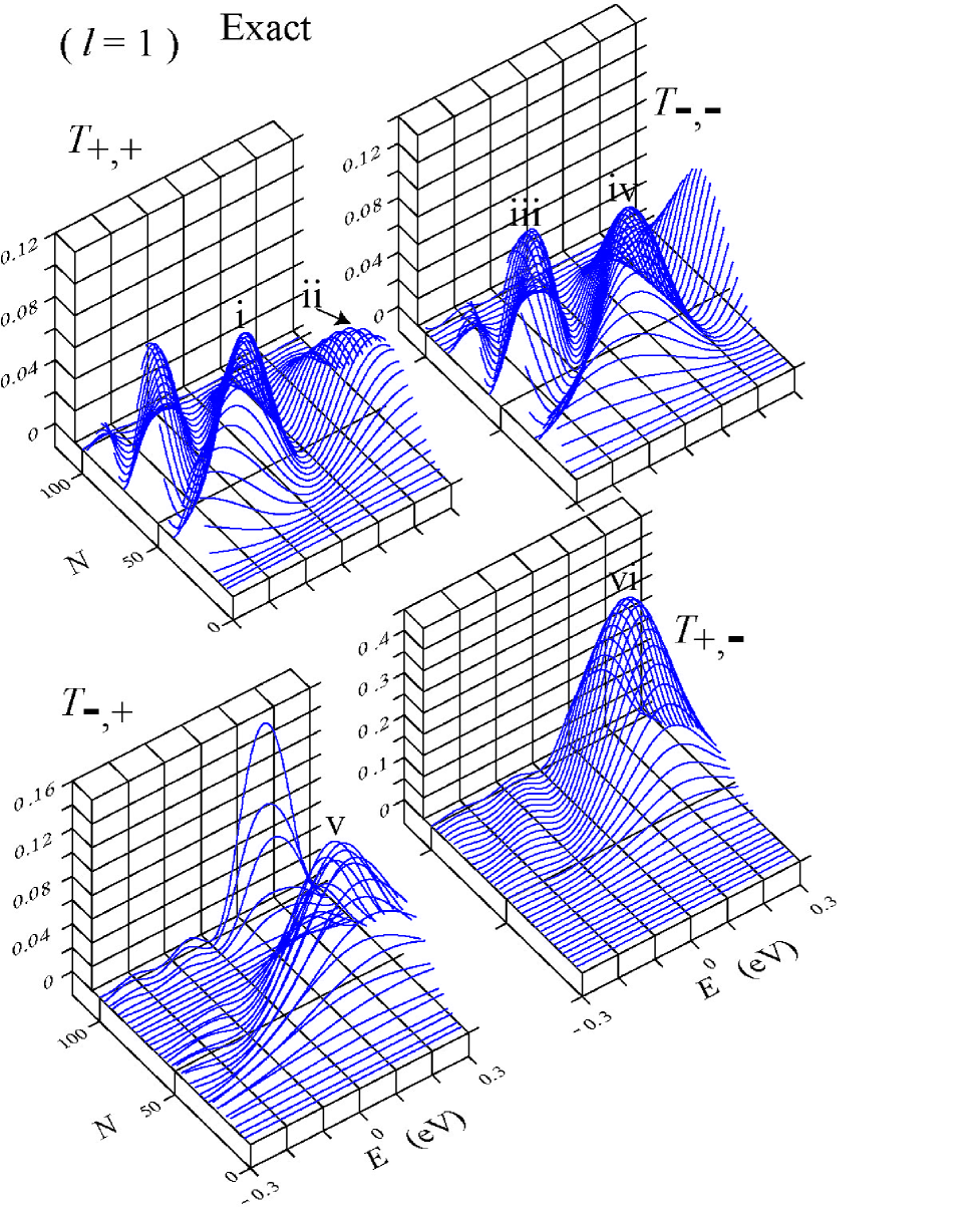
FIG. 9.: The exact numerical data corresponding to Fig. 8. The local maximums are compared with those of Fig. 8 in Table III.

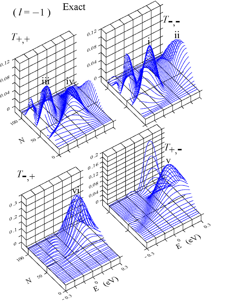
FIG. 10.: The same numerical data as in Fig. 9 except the residue $l=-1$. The local maximums are compared with those of Fig. 8 in Table III. The data $T$ of Fig. 8 are transformed by Eq. (66) and shown in the rightmost column of Table III.

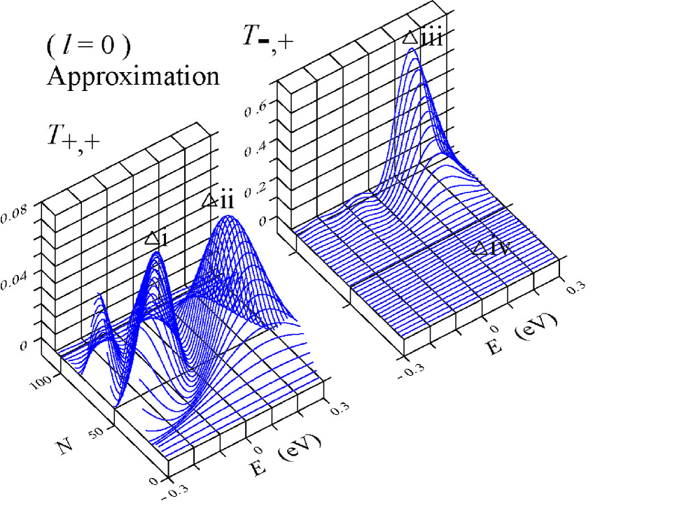
FIG. 11.: Three dimensional view of Eqs. (52) and (55) in case $l=0$, $\varepsilon=$ 0.3 eV, $\theta_{\rm d}=0$ and $z_{\rm d}=0$.

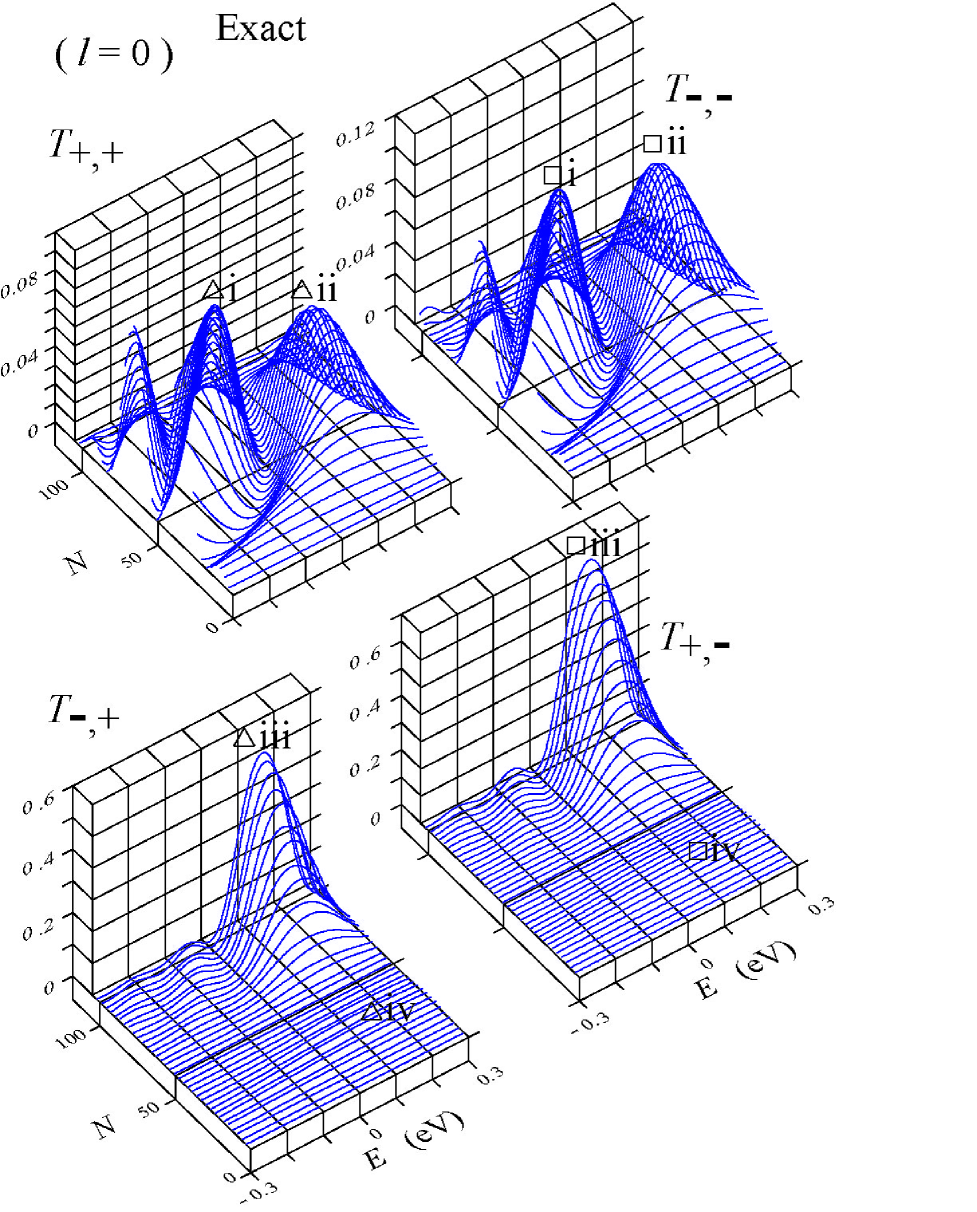
FIG. 12.: The same numerical data as in Fig. 9 except the residue $l=0$. The local maximums are compared with those of Fig. 11 in Table III. The data $T$ of Fig. 11 are transformed by Eq. (66) and shown in the rightmost column of Table IV.

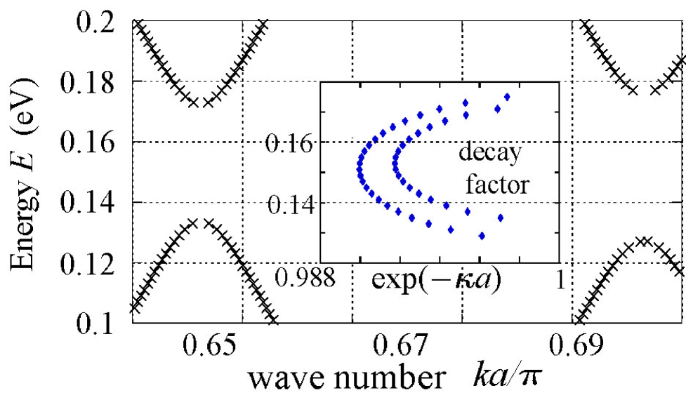
FIG. 13.: (main panel) The exact dispersion relation near the corner point. (inset) The decay factors $e^{-\kappa a}$.

FIG. 14.: (a) $T_{\sigma,\sigma}$ and (b) $T_{-\sigma,\sigma}$ at $E=\varepsilon/2=0.15$ eV in case $l=1$. The exact and approximate results are shown by the solid and dashed lines, respectively. Black and grey lines correspond to $\sigma=+$ and $\sigma=-$, respectively. The neighboring peaks indicated by arrows show the exponential decay of the gap state. At the vertical line with $\triangleright$ ($\triangleleft$), the VCF and the VCR manifest themselves as $T_{+,-}>0.9$ and $T_{-,+}<0.1$ ($T_{-,+}>0.9$ and $T_{+,-}<0.1$).

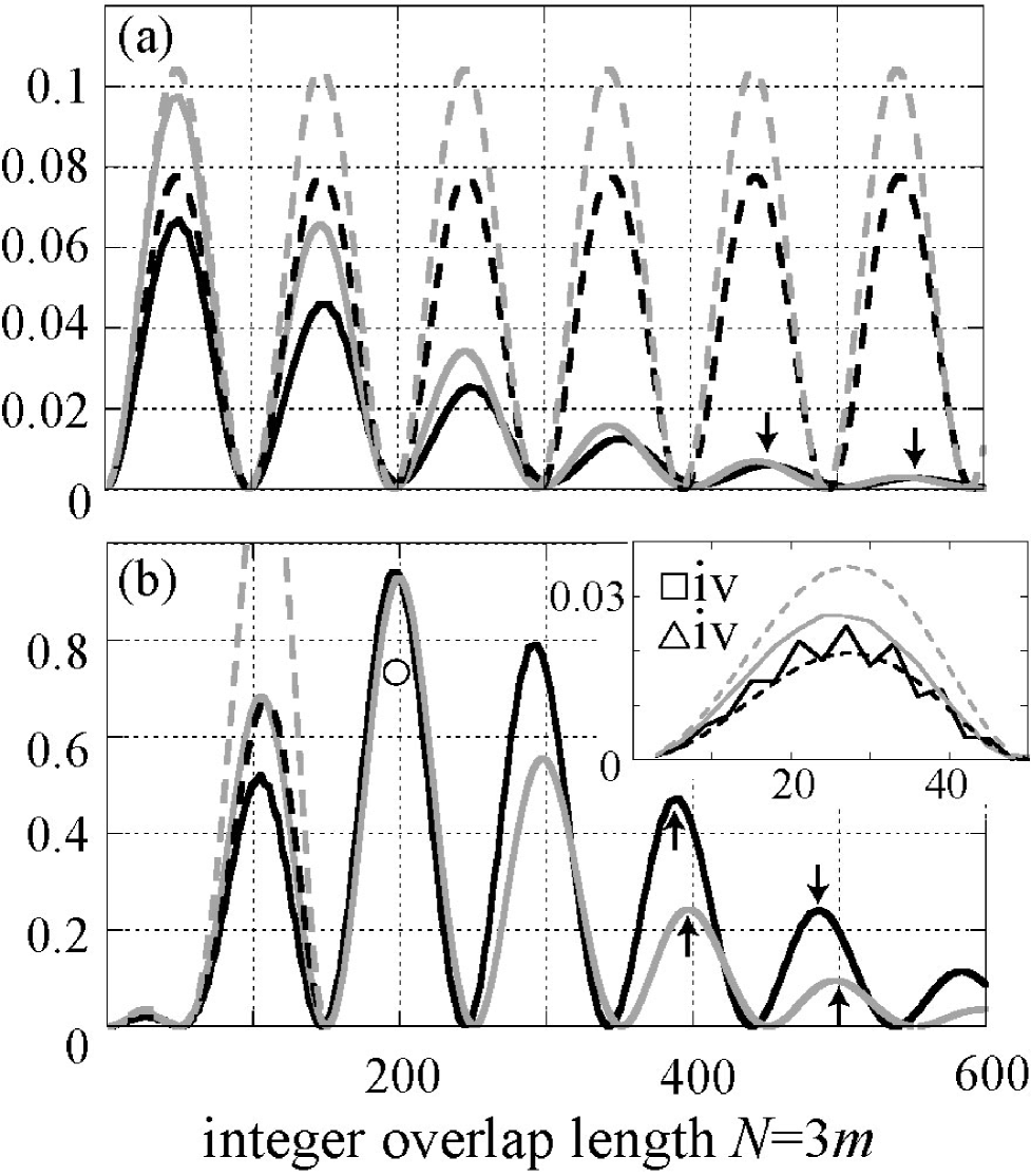
FIG. 15.: The same as Fig. 15 except $l=0$. At the peak with $\circ$, the VCR manifest itself as $T_{+,-}\simeq T_{-,+}>0.9$.

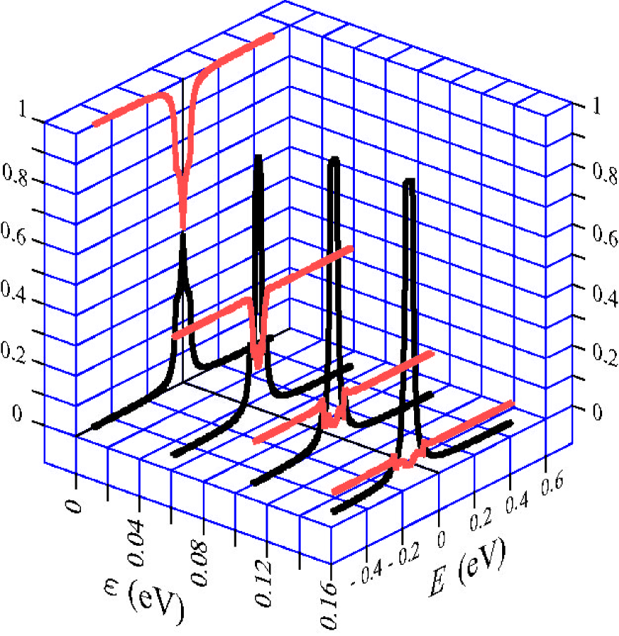
FIG. 16.: The product of the squared overlap integrals defined by Eq. (63) where $t_{\bot}=$ 0.04 eV and $\varepsilon=$ 0, 0.05, 0.1, 0.15 eV. The black and red lines indicate $I_{+,-}$ and $I_{+,+}$, respectively.

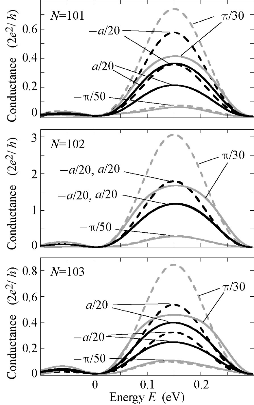
FIG. 17.: The Landauer’s formula conductance $G=(2e^{2}/h)\sum_{\sigma,\sigma^{\prime}}T_{\sigma^{\prime},\sigma}$ in case $(\theta_{\rm d},z_{\rm d})=(0,\pm a/20),(-\pi/50,0),(\pi/30,0)$, $N=$ 101, 102, 103. The black and gray lines correspond to $\theta_{\rm d}=0$ and $z_{\rm d}=0$, respectively. The dashed lines correspond to Eqs. (52) and (55) . The solid lines indicate the exact results.

REFERENCES

- [1] S. A. Vitale, D. Nezich, J. O. Varghese, P. Kim, N. Gedik, P. Jarillo-Herrero, D. Xiao, and M. Rothschild, Small 14, 1801483 (2018);M. B. Lundeberg and J. A. Folk, Science 346, 422 (2014).
- [2] Y. J. Zhang, T. Oka, R. Suzuki, J. T. Ye, and Y. Iwasa, Science 344, 725 (2014); K. F. Mak, K. L. McGill, J. Park, P. L. McEuen, Science 344, 1489 (2014).
- [3] Y. Jiang, T. Low, K. Chang, M. I. Katsnelson, and F. Guinea, Phys. Rev. Lett. 110, 046601 (2013); Y. Shimazaki, M. Yamamoto, I. V. Borzenets, K. Watanabe, Y. Taniguchi, and S. Tarucha, Nature Phys. 11, 1032 (2015).
- [4] S. Das Sarma, S. Adam, E. H. Hwang, and E. Rossi, Rev. Mod. Phys. 83, 407 (2011); A. H. Castro Neto, F. Guinea, N. M. R. Peres, K. S. Novoselov, and A. K. Geim, ibid. 81, 109 (2009).
- [5] H. Schomerus, Phys. Rev. B 82, 165409 (2010).
- [6] M. Settnes, S. R. Power, M. Brandbyge, and A-P. Jauho, Phys. Rev Lett. 117, 276801 (2016).
- [7] Y. Liu, J. Song, Y. Li, Y. Liu, and Q. F. Sun, Phys. Rev. B 87, 195445 (2013); J.-H. Chen, G. Autes, N. Alem, F. Gargiulo, A. Gautam, M. Linck, C. Kisielowski, O. V. Yazyev, S. G. Louie, and A. Zettl, ibid. 89 , 121407(R) (2014); D. Gunlycke and C. T. White, Phys. Rev. Lett. 106, 136806 (2011).
- [8] S. K. Wang and J. Wang, Phys. Rev. B 92, 075419 (2015); J. J. Wang, S. Liu, J. Wang, and J. -F. Liu, ibid. 98, 195436 (2018); C. W. J. Beenakker, N. V. Gnezdilov, E. Dresselhaus, V. P. Ostroukh, Y. Herasymenko, I. Adagideli, and J. Tworzydlo, ibid. 97, 241403(R) (2018);F. Xu, Z. Yu, Y. Ren, B. Wang, Y. Wei, and Z. Qiao, New J. Phys. 18 113011 (2016).
- [9] R. Li, Z.Lin, and K. S. Chan, Physica E 113, 109 (2019).
- [10] J.-C. Charlier, X. Blase, and S. Roche, Rev. Mod. Phys. 79, 677 (2007); E. A. Laird, F. Kuemmeth, G. A. Steele, K. Grove-Rasmussen, J. Nygård, K. Flensberg, and L. P. Kouwenhoven, ibid. 87, 703 (2015).
- [11] C. Buia, A. Buldum, and J. P. Lu, Phys. Rev. B 67, 113409 (2003); M. A. Tunney and N. R. Cooper, ibid. 74, 075406 (2006); A. Hansson and S. Stafstrom, ibid. 67, 075406 (2003); I. M. Grace, S. W. Bailey, and C. J. Lambert, ibid. 70, 153405 (2004);Y.-J. Kang, K. J. Chang, and Y.-H. Kim, ibid. 76, 205441 (2007); R. Tamura, Y. Sawai, and J. Haruyama, ibid. 72, 045413 (2005);D.-H. Kim and K. J. Chang, ibid. 66, 155402 (2002);S. Uryu and T. Ando, Phys. Rev. B 76, 155434 (2007);72, 245403 (2005); Q. Liu, G. Luo, R. Qin, H. Li, X. Yan, C. Xu, L. Lai, J. Zhou, S. Hou, E. Wang, Z. Gao, and J. Lu, ibid. 83, 155442 (2011); A. Buldum and J. P. Lu, ibid. 63, 161403(R) (2001); Q. Yan, G. Zhou, S. Hao, J. Wu, and W. Duan, Appl. Phys. Lett. 88, 173107 (2006); S. Tripathy and T. K. Bhattacharyya, Physica E 83, 314 (2016).
- [12] R. Tamura, Phys. Rev. B 82, 035415 (2010).
- [13] R. Tamura, Phys. Rev. B 86, 205416 (2012).
- [14] R. Tamura, Phys. Rev. B 99, 155407 (2019).
- [15] F. Xu, A. Sadrzadeh, Zhiping Xu, and B. I. Yakobson, J. Appl. Phys. 114, 063714 (2013).
- [16] J. Cumings and A. Zettl, Science 289, 602 (2000); A. Kis, K. Jensen, S. Aloni, W. Mickelson, and A. Zettl, Phys. Rev. Lett. 97, 025501 (2006); Q. Zheng and Q. Jiang, ibid. 88, 045503 (2002); S. B. Legoas, V. R. Coluci, S. F. Braga, P. Z. Coura, S. O. Dantas, and D. S. Galvao, ibid. 90, 055504 (2003); W. Guo, Y. Guo, H. Gao, Q. Zheng, and W. Zhong, ibid. 91, 125501 (2003); P. Tangney, M. L. Cohen, and S. G. Louie, ibid. 97, 195901 (2006); J. Cumings and A. Zettl, ibid. 93, 086801 (2004); J. Servantie and P. Gaspard, Phys. Rev. B 73, 125428 (2006); Phys. Rev. Lett. 91, 185503 (2003); Q. Zheng, J. Z. Liu, and Q. Jiang, Phys. Rev. B 65, 245409 (2002); S. Akita and Y. Nakayama, J. J. Appl. Phys. 42, 4830 (2003); M. Nakajima, S. Arai, Y. Saito, F. Arai, and T. Fukuda, ibid. 46, L1035 (2007); W. Zhang, Z. Xi, G. Zhang, C. Li, and D. Guo, Phys. Chem. Lett. 112, 14714 (2008); J. W. Kang and O. K. Kwon, Appl. Sur. Sci. 258, 2014 (2012).
- [17] A. A. Tonkikh, V. I. Tsebro, E. A. Obraztsova, K. Suenaga, H. Kataura, A. G. Nasibulin, E.I. Kauppinen, and E. D. Obraztsova, CARBON 94, 768 (2015); V. I. Tsebro, A. A. Tonkikh, D. V. Rybkovskiy, E. A. Obraztsova, E. I. Kauppinen, and E. D. Obraztsova, Phys. Rev. B 94, 245438 (2016).
- [18] R. Nakanishi, R. Kitaura, P. Ayala, H. Shiozawa, K. de Blauwe, P. Hoffmann, D. Choi, Y. Miyata, T. Pichler, and H. Shinohara, Phys.Rev. B 86, 115445 (2012).
- [19] E. R. Margine and Vincent H. Crespi Phys. Rev. Lett. 96, 196803 (2006); T. Miyake and S. Saito, Phys. Rev. B, 65, 165419 (2002).
- [20] D. A. Bandurin, I. Torre, R. Krishna Kumar, M. Ben Shalom, A. Tomadin, A. Principi, G. H. Auton, E. Khestanova, K. S. Novoselov, I. V. Grigorieva, L. A. Ponomarenko, A. K. Geim, and M. Polini, Science 351, 1055 (2016). A. I. Berdyugin, S. G. Xu, F. M. D. Pellegrino, R. Krishna Kumar, A. Principi, I. Torre, M. Ben Shalom, T. Taniguchi, K. Watanabe, I. V. Grigorieva, M. Polini, A. K. Geim, and D. A. Bandurin, Science 364, 162 (2019); Z. Wang, H. Liu, H. Jiang, and X. C. Xie, Phys. Rev B 100, 155423 (2019).
- [21] T. Aktor , J. H. Garcia, S. Roche, A. P. Jauho, and S. R. Power, Phys.Rev. B 103, 115406 (2021); G. Kirczenow,ibid, 92, 125425 (2015).
- [22] Y. J. Dappe, J. Ortega, and F. Flores, Phys. Rev. B 79, 165409 (2009); C. Li, Y. Liu, X. Yao, M. Ito, T. Noguchi, and Q. Zheng, Nanotech. 21 , 115704 (2010).
- [23] Ph. Lambin, V. Meunier, and A. Rubio, Phys. Rev. B 62, 5129 (2000); J. -C. Charlier, J. -P. Michenaud, and Ph. Lambin, ibid. 46, 4540 (1992).
- [24] A. A. Farajian, K. Esfarjani, and Y. Kawazoe, Phys. Rev. Lett. 82, 5084 (1999).
- [25] S. Datta, Electronic Transport in Mesoscopic Systems (Cambridge University Press, Cambridge 1995).
- [26] R. V. Gorbachev, J. C. W. Song, G. L. Yu, A. V. Kretinin, F. Withers, Y. Cao, A. Mishchenko, I. V. Grigorieva, K. S. Novoselov, L. S. Levitov, and A. K. Geim, Science 346, 448 (2014); J. H. J. Martiny , K. Kaasbjerg, and A. -P. Jauho, Phys. Rev. B 100, 155414 (2019); K. Komatsu, Y. Morita, E. Watanabe, D. Tsuya, K. Watanabe, T. Taniguchi, and S. Moriyama, Sci. Adv. 4, eaaq0194 (2018); D. Xiao, W. Yao, and Q. Niu, Phys. Rev. Lett 99, 236809 (2007);M. Yamamoto, Y. Shimazaki1, I. V. Borzenets, and S. Tarucha, J. Phys. Soc. Jpn 84, 121006 (2015).
- [27] J. J. Sakurai, Modern quantum mechanics (Addison-Wesley, Tokyo, 1994).
- [28] The notations and in Ref. [12] are represented by with the notations of the present paper. Here is limited to odd integers in Ref. [12] while we consider both odd and even in the present manuscript. Since the rapid oscillation is suppressed in the average , can be approximated by when .