Gamma–rays from kilonovae and the cosmic gamma–ray background

Abstract

The recent detection of the gravitational wave event GW170817, produced by the coalescence of two neutron stars, and of its optical–infrared counterpart, powered by the radioactive decay of r–process elements, has opened a new window to gamma–ray astronomy: the direct detection of photons coming from such decays. Here we calculate the contribution of kilonovae to the diffuse gamma–ray background in the MeV range, using recent results on the spectra of the gamma–rays emitted in individual events, and we compare it with that from other sources. We find that the contribution from kilonovae is not dominant in such energy range, but within current uncertainties, its addition to other sources might help to fit the observational data.

1. Introduction

Up to this day, there is no clear understanding of which sources or emission mechanisms may account for the MeV background (de Angelis et al., 2018; Ajello et al., 2019; Tatischeff et al., 2019; McEnery et al., 2019). On the low–energy side, from X–ray energies up to around 0.3 MeV, AGNs and Seyfert galaxies provide most of the emission (Madau et al., 1994; Ueda et al., 2003), but these contributions sharply cut off at $E\hbox{\lower 3.44444pt\hbox{$\,\buildrel>\over{\sim}\,$}}0.3$ MeV. At energies in the 50 MeV to the GeV range, blazars, star–forming galaxies and radio galaxies can explain the observed background (Ajello et al., 2015; Di Mauro & Donato, 2015).

A potential candidate for the missing source of MeV photons could be associated with the sites of heavy-element nucleosynthesis. However, the sites of the nucleosynthesis of heavy elements produced by rapid sequences of neutron captures, the r–process elements, has long been a matter of debate. The innermost parts of the ejecta from gravitational–collapse supernovae (Woosley et al., 1994), material expelled in the coalescence of two neutron stars (NSs) or of a NS and a black hole (BH) (Lattimer & Schramm, 1974), and jets from magnetorotationally-driven supernovae (Winteler et al., 2012) have been proposed. In this study, we focus on the neutron star mergers and the gamma emission they can produce.

Li & Paczyński (1998) were first to propose that the merger of two NSs should produce an electromagnetic transient, later named “macronova” (Kulkarni, 2005) or “kilonova” (KN being the currently most used term), powered by the radioactive decay of the merger debris and seen in optical and infrared bands (Metzger et al., 2010). Such debris would be rich in r–process elements and their radioactivity would heat the ejected material and make it luminous. Subsequent studies of the heating rates (Metzger & Berger, 2012; Korobkin et al., 2012; Lippuner & Roberts, 2015) found that the late–time bolometric light curve of the KN would provide evidence of the radioactive material and enable to estimate the amount of r–process elements produced in the merger. A re–analysis of the afteglow light curves of nearby short gamma–ray bursts (sGRBs) by Jin et al. (2016), now generally attributed to the merger of two NSs (Eichler et al., 1989; Nakar, 2007; Berger, 2014), suggests that KNe are always present in the afterglows of the sGRBs (see also Tanvir et al., 2013; Kasliwal et al., 2017).

The detection of GW170817, the gravitational wave signal of a binary NS inspiral (Abbott et al., 2017) was followed by the discovery of an electromagnetic counterpart, a KN (Arcavi et al., 2017; Coulter et al., 2017; Lipunov et al., 2017; Pian et al., 2017; Soares-Santos et al., 2017; Tanvir et al., 2017; Valenti et al., 2017), known as DLT17ck (and also as SSS17a and as AT 2017gfo). A sGRB (GRB 170817A), consistent with the gravitational wave signal location, was also detected, two seconds later, by the Gamma–Ray Burst Monitor aboard the Fermi spacecraft (Goldstein et al., 2017). A second event, GW190425, also corresponds to the merger of two NSs (Abbott et al. 2020). A sGRB, GRB 190425, was detected with the gamma–ray spectrometer SPI aboard the INTEGRAL observatory (Pozanenko et al. 2019), but no observations are available at other wavelengths.

The observations of the KN associated with GW170817 show that, as predicted, it originated from neutron–rich matter unbound from the system (McCully et al., 2017; Smartt et al., 2017; Rosswog et al., 2018). Two distinct components of the KN were clearly identified: an early blue KN, peaking in optical bands (Evans et al., 2017), and a late, infrared KN (Tanvir et al., 2017). The blue peak would be produced by a disk–driven wind enriched with lighter r–process elements (Kasliwal et al. 2017), while the more slowly evolving infrared emission would be powered by the decay of the lanthanide–rich material, dynamicallly ejected at the merger. This is in agreement with the theory, which predicts that the dynamical ejecta from mergers will produce lanthanide-rich composition and peak in the infrared, while secondary postmerger outflows will result in a less neutron-rich composition, leading to lighter r–process without lanthanides (Kasen et al., 2013; Barnes & Kasen, 2013; Grossman et al., 2014). In this study, we employ a similar two–component model for gamma–ray emission: very neutron–rich “dynamical ejecta” and “wind”, their emission lasting for about one month (further details in Section 3).

Gamma–rays are emitted by the ejecta at all epochs. They fall, as in the case of Type Ia supernovae (SNe Ia), within the MeV range, precisely a region of the cosmic gamma–ray background spectrum where there are no known sources that satisfactorily fit the observations (Ajello et al., 2019). For the production of gamma–rays, here we consider both the “kilonova” phase lasting for about a month, and a “remnant” phase, due to long-lived residual nuclides from the r-process, and extending up to $\sim$ 10⁶ years (see KorBobkin et al., 2019).

In previous studies, Hotokezaka et al. (2016) pioneered detailed computation of the gamma-ray spectra from kilonovae. They used a line-broadening approach to simulate the ejecta expansion with subrelativistic speeds (appropriate for epochs earlier than about one week since the merger). Li (2019) extended the calculation of the spectrum with a semi-analytic model for radiative transport and nuclear decay chains. In KorBobkin et al. (2019), we used a full 3D Monte Carlo radiative transport code (Hungerford et al., 2003, 2005) to simulate the emission in the kilonova phase, and a simple line broadening to extend the emission spectra to the remnant state (over 100 kyr). In this study, we apply the computed spectra at both phases to derive the contribution of KNe to the diffuse gamma–ray background. We will see that KNe do not appear to give a dominant contribution to the background but, within current uncertainties, might, together with that from SNe Ia, improve the fit to the observational data when added to another, dominant source.

The paper is organized as follows: first we deal with the KN rates in Section 2 and in Section 3 with the r–elements yields. The observations of the gamma–ray background in the MeV range are presented in Section 4. The input gamma–ray spectra and the method used to calculate the KN background are described in Section 5. The results are presented and discussed in Section 6. Section 7 summarizes the present study, gives its conclusions and points to ways for improvements.

2. The kilonova rates

The rates of KN engines — neutron star mergers — have been estimated theoretically in multiple studies (e.g. Kalogera et al., 2004b, a; Kim et al., 2015; Wanderman & Piran, 2015). Abbott et al. (2020), from the detections of GW170817 and GW190425, infer a rate of 1090${}^{+1720}_{-800}$ Gpc^-3 yr^-1. For that rate, as we will see, the kilonova contribution to the gamma–ray background would be very minor. But, as noted by Della Valle et al. (2018), the rate of NS–NS mergers is still very poorly constrained. Recently, Yang et al. (2017), based on the light curve of AT 2017gfo/DLT17ck (the electromagnetic counterpart of GW170817) and on the results of the DLT Supernova search, set an upper limit of $0.99\times 10^{-4}\ {}^{+0.19}_{-0.15}$ Mpc^-3 yr^-1 to the local rate ($d<40$ Mpc) of binary NS mergers. We will use it as our reference rate, but we equally consider the upper and lower limit given by Abbott et al. (2020).

For calculating the contribution of KNe to the cosmic gamma–ray background, we need to estimate how the rates have varied along $z$. Massive stars promptly become neutron stars, but there can be a considerable time interval between the formation of binary systems made of two NSs and the merger of the two objects. Wanderman & Piran (2015) find that there is a delay of 3–4 Gyr of the mergers relative to the global star formation rate.

For the cosmic star formation rate, we use the results of Cucciati et al. (2012). We derive the binary neutron star coalescence rate assuming an average delay time of 3.5 Gyr and we normalize the rates to the upper limit set by Yang et al. (2017) to the local rate. The resulting KN rate, $R_{KN}(z)$ (Mpc^-3 yr^-1), is shown in Figure 1.

Figure 1.— The KN rate as a function of redshift $z$, for an average time delay of 3.5 Gyr between star formation and NS–NS mergers, based on the cosmic star formation rate of Cucciati et al. (2012), normalized to the upper limit to the local KN rate set by Yang et al. (2017).

3. The r–process yields from kilonovae

As pointed out in the Introduction, NS–NS mergers are main candidates to the production of the r–process elements. Their relevance in this respect depends on the rate of the mergers and on the amount of r–process elements produced in each event. We have dealt with the first point in the previous Section.

Concerning the second point, the amount and composition of the ejecta depend on how and when during the merger the material has become unbound (for a review, see Metzger, 2019). The most neutron-rich component known as “dynamical ejecta” gets unbound by dynamical tide and attains ideal conditions for robust r–process nucleosynthesis (Freiburghaus et al., 1999; Korobkin et al., 2012; Bauswein et al., 2013). Other types of ejecta include the material “squeezed” from the binary contact interface (Goriely et al., 2011; Wanajo et al., 2014), neutrino-driven outflows from the merged hypermassive neutron star (Dessart et al., 2009; Perego et al., 2014), from the accretion disk (Fernández et al., 2015; Miller et al., 2019), or fallback material (Desai et al., 2019). These types may produce full r–process but in general are not expected to produce robust, main r–process nucleosynthesis due to their lack of mechanism to ensure high neutron richness, necessary for fission cycling (Holmbeck et al., 2019).

Observationally, ejecta can be classified into two types: lanthanide-rich ejecta producing the late “(infra-)red” KN, and lanthanide-poor component, responsible for the “blue” KN (Metzger, 2019). Below, we will refer to these two components as “dynamical ejecta” and “wind”, and use representative compositions described in KorBobkin et al. (2019) (see their Fig. 3 and Table 1). Regarding the masses, theoretical estimates vary around $10^{-2}$ M_⊙ within about two orders of magnitude (Hotokezaka et al., 2013; Bauswein et al., 2013; Radice et al., 2016; Dietrich & Ujevic, 2017). Theoretical models for GW170817 give a similar range of estimates for the two components, as shown in Table 1 of Côté et al. (2018) (see also Ji et al., 2019, for more complete summary). Somewhat higher values were deduced for previous afterglow excess events (Tanvir et al., 2013; Piran et al., 2014; Jin et al., 2016; Wollaeger et al., 2018), although here a selection effect might play a role.

In this study, we adopt a conservative range from 10^-4 M_⊙ to 0.1 M_⊙ for both ejecta components, to cover the described uncertainties.

4. The observed diffuse gamma–ray background

Figure 2.— The diffuse gamma–ray background in the MeV range, as measured by the Solar Maximum Mission (solid line, dotted lines being the 1 $\sigma$ upper and lower limits: Watanabe et al., 1999) and by COMPTEL (black squares: Kappadath et al., 1996).

The present measurements of the gamma–ray background in the MeV range (from 100 keV to 10 MeV) mostly come from two space missions: the Solar Maximum Mission (SMM; Watanabe et al., 1999) and COMPTEL (Kappadath et al., 1996; Weidenspointner, 1999; Weidenspointner et al., 2000). More recent gamma–ray missions, either have not covered this energy range (like Fermi) or have not yet produced available data on the background (like INTEGRAL). The measurements are shown in Figure 2. As we see, the slope of the emission spectrum has a steep decrease with increasing energy, from a few hundred keV to 10 MeV (flux $\propto E^{-2.5}$, approximately). It changes to a flatter slope around 10 MeV and beyond. An intense extragalactic source (or the addition of several) is needed in the MeV window (see, for instance, Lacki et al., 2014).

As we have seen, the gamma–ray emission from KNe, both in their dynamical and remnant stages, falls within the above range, hence the interest of modeling their contribution to the diffuse background emission.

5. Modeling the kilonova gamma–ray background

To calculate the KN contribution to the diffuse gamma–ray background, we integrate the evolving luminosity over the time in which the ejecta appreciably emit gamma–rays. First we will consider the contribution in the KN phase, which includes the dynamical and wind components This phase lasts for about a month. Afterwards, we add the contribution from the remnant phase, extending up to $\sim 10^{6}$ yr. We use the spectra of four models, calculated in KorBobkin et al. (2019) (see their Fig. 4): the evolution of these spectra over 32 days is reproduced in Figure 3, for their model labeled Ak (see Table 1 in KorBobkin et al., 2019). This model represents a very neutron-rich outflow with, generating the main (robust) r-process through fission cycling. We have checked that for the remaining three models As, S1 and S2 the resulting contributions to the background are very similar. Our standard case corresponds to their adopted values for the mass ejected: 0.0065 M_⊙ in the dynamical ejecta component and 0.03 M_⊙ in the wind component. Given the wide range of ejected masses derived from the observations of GW170817 by different authors (see Section 3 above) we also calculate the KN background for both the highest and the lowest masses in the range, in order to obtain an idea of its upper and lower limits. We are aware of the roughness of our treatment, since scaling the emission by the mass of the ejecta neglects the change in material opacity to the gamma–rays in KN phase, and a full calculation of the spectra should instead be made for each case. However, the effect of a finite opacity is significant only at the initial epoch of a day or so, and should be subdominant to the range of mass uncertainty.

The spectra for the remnant phase of the model Ak are shown in Figure 4. Here the ejecta is practically transparent and no transport calculation is needed. To obtain the spectra at different times, we computed the detailed nuclear gamma–ray source using Eq. (1) in KorBobkin et al. (2019) and applied Doppler broadening with typical remnant expansion velocities for each epoch (see Fig. 6 in KorBobkin et al., 2019). The Figure 4 also compares the Doppler-broadened spectrum with the spectrum from the full radiative transfer model (dashed line) at $t=32$ days. Two spectra show an excellent agreement, demonstrating the validity of our approach for the remnant phase.

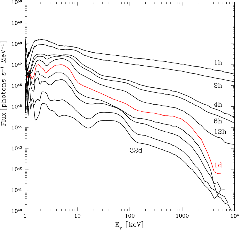
Figure 3.— Evolution of the gamma–ray spectra in the KN phase, up to 32 days after a NS–NS merger, computed with 3D radiative transfer code for the neutron-rich dynamical ejecta model Ak (from KorBobkin et al., 2019, see their Table 1).

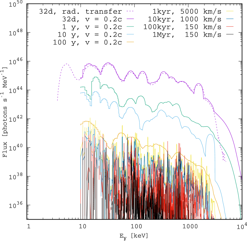
Figure 4.— Evolution of the gamma–ray spectra in the remnant phase, from 32 days up to 10⁶ yr, for the neutron-rich dynamical ejecta model Ak. For each solid line, the detailed isotopic decay spectrum is Doppler-broadened with the remnant expansion velocity typical for the remnant phase at this epoch (shown in the legend). The dashed line represents the full radiative transfer model Ak at $t=32$ days, in good agreement with the Doppler-broadened spectrum.

To model the contribution of KN to the cosmic gamma-ray background, we follow the same steps as in Ruiz-Lapuente et al. (2016) when modeling that from SNe Ia. First, from the gamma–ray emission at different stages in the evolution of the ejecta, we infer the total number of photons emitted (photons keV^-1) in each event, and dividing by its duration, $\tau_{KN}$ (taken as 32 days for the KN phase and as $10^{6}$ yr for the remnant phase), the average luminosity, $l_{\gamma}(E)$ (photons s^-1 keV^-1) is obtained. The number of KNe per unit of comoving volume, $R^{\prime}_{KN}(z)$, active at any time, is that of the KN produced during the previous time interval of duration $\tau_{KN}$, so: ${R^{\prime}_{KN}(z)={\rm const}\times R_{KN}(z)}$, the latter being the comoving KN rate (KN yr^-1 Mpc^-3) and, for the KN phase, ${\rm const}=32/365.25=0.0876$, while for the remnant phase ${\rm const}=10^{6}$. The contribution to the gamma–ray background of the shell at comoving radius $r$ and with thickness $dr$ is:

$$dL_{\gamma}(E,z)=4\pi R^{\prime}_{KN}(z)l_{\gamma}(E)dV(z)$$ (1)

where

$$dV(z)=D_{M}^{2}(z)dD_{M}$$ (2)

$D_{M}$ being the proper motion distance (in Mpc). The flux received from that shell (photons cm^-2 s^-1 keV^-1) will be:

$$dF_{\gamma}(E,z)={\frac{1}{4\pi}D_{L}(z)^{2}}dL_{\gamma}[(z+1)E,z]$$ (3)

$D_{L}$ being the luminosity distance (cm). The factor ${(z+1)}$, multiplying $E$, accounts for the redshift of the photons. Then we have:

$$dF_{\gamma}(E,z)=R^{\prime}_{KN}(z)l_{\gamma}[(z+1)E]{D_{M}^{2}(z)\over D_{L}^{2}(z)}dD_{M}$$ (4)

Due to time dilation, there should be a factor ${(1+z)^{-1}}$ multiplying the comoving KN rate, but it is canceled by the ${(z+1)}$ factor accounting for compression of the energy bins. Since ${D_{L}=(1+z)D_{M}}$, we have

$$dF_{\gamma}(E,z)={1\over(1+z)^{2}}R^{\prime}_{KN}(z)l_{\gamma}[(z+1)E]dD_{M}$$ (5)

$dD_{M}$ depends on the cosmological parameters $H_{0}$, $\Omega_{M}$ and $\Omega_{\Lambda}$, so we finally have:

$$\begin{split}F_{\gamma}(E)={c\over H_{0}}\int_{0}^{z_{\rm lim}}{{1\over(1+z)^{2}}R^{\prime}_{KN}l_{\gamma}[(z+1)E]}\\ \times e(z,\Omega_{M},\Omega_{\Lambda})dz\end{split}$$ (6)

We adopt $H_{0}$ = 67 km s^-1 Mpc^-1, ${\Omega_{M}=0.31}$ and ${\Omega_{\Lambda}=0.69}$, from the Planck Collaboration & et al. (2018), assuming a flat universe. The last term in the previous equation is:

$$e(z,\Omega_{M},\Omega_{\Lambda})=[(1+z)^{2}(1+\Omega_{M}z-z(2+z)\Omega_{\Lambda}]^{-1/2}$$ (7)

In order to compare the calculated fluxes with observations, we must divide the $F_{\gamma}(E)$ above by 4$\pi$, to convert to the units used in reporting observed fluxes (photons cm^-2 s^-1 keV^-1 sr^-1).

6. Results and discussion

In Figure 5, the contributions of mergers in their KN phase to the diffuse gamma–ray background in the 10 keV – 10 MeV range are compared with the available observations. The continuous black line corresponds to our “standard” case, and the two dotted red lines to our adopted upper and lower limits for the ejected mass. The two blue, slashed lines correspond to the upper and lower limits to the local merger rate set by Abbott et al. (2020), for the “standard” ejecta masses, while the red dot–dashed line is for the combination of their upper limit on the merger rate with that on the ejected mass. We see that, for energies $E_{\gamma}$ between roughly 200 keV and 3 MeV, the slope of the contribution follows that of the data, but at significantly lower values of the fluxes, even for our “standard” upper limit, than the observed ones. If we compare with the contribution from SNe Ia (which is made in Figure 7), we have that KNe have a higher average luminosity $l_{\gamma}$ than SNe Ia, but that is countered by the fact of the shorter duration of the KNe in this phase (32 days against 600 days) and by their lower rate of occurrence.

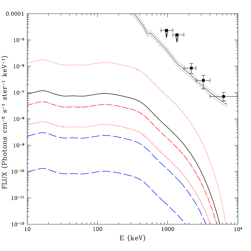
Figure 5.— The contributions of NS–NS mergers to the cosmic gamma–ray background in the MeV range, due to the emission of the ejecta in KN phase, calculated from the spectra in Figure 3, for the standard ejecta masses (black continuous line) and for the maximum (${0.1\,M_{\odot}}$) and minimum (${10^{-4}\,M_{\odot}}$) masses in the range (red dotted lines). They are compared with the observations (continuous black line: Solar Maximum Mission, from Watanabe et al. (1999), dotted lines being the 1 $\sigma$ upper and lower limits; black squares: COMPTEL, from Kappadath et al. (1996)). The two blue, dashed lines correspond to the upper and lower limits to the local NS–NS merger rate set by Abbott et al. (2020), and the red dot–dashed line to the combination of their upper limit on the KN rate with that on the ejected mass.

In Figure 6, we plot the contribution to the background by NS–NS merger ejecta in their remnant phase, also the “standard” one (continuous red line) and upper and lower limits estimated as above. The average luminosity $l_{\gamma}$ is lower than in the KN phase, that being partially compensated by the long duration of the phase. The contributions calculated for the upper and lower limits to the local KN rate from Abbott et al. (2020) are indicated by the blue dashed lines, while the dot–dashed one corresponds to the combination of their upper limit on the merger rate with that on the ejected mass of radioactive nuclei.

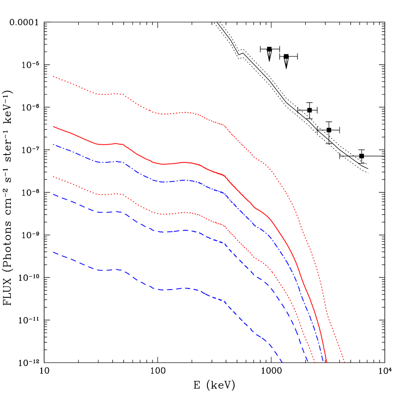
Figure 6.— Similar to Figure 5, with the contribution of NS–NS mergers due to the emission of the ejecta in their remnant phase (red continuous line) and its upper and lower limits (red dotted lines), calculated from the spectra in Figure 4. Also shown, by the blue dashed lines, are the contributions calculated for the upper and lower limits to the local NS–NS merger rate from Abbott et al. (2020). As in the previous Figure, the dot–dashed line corresponds to the combination of their upper limit on the KN rate with that for the mass of the ejecta.

In Figure 7, the KN backgrounds (“standard” and upper and lower limits) for all phases are compared with that from SNe Ia (dashed line, adopted from Ruiz-Lapuente et al., 2016). We also show the result (dot–dashed blue line in the Figure) of adding our upper limit to the KN contribution to that of the SNe Ia. Equally shown, again, are the backgrounds corresponding to the upper and lower limits to the local KN rate from Abbott et al. (2020) and the combination of that upper limit with the highest estimate of the mass of the KN ejecta. The coincidence of the slope of the KN contribution with that of the measured background is remarkable, although it remains significantly below even at its upper limit.

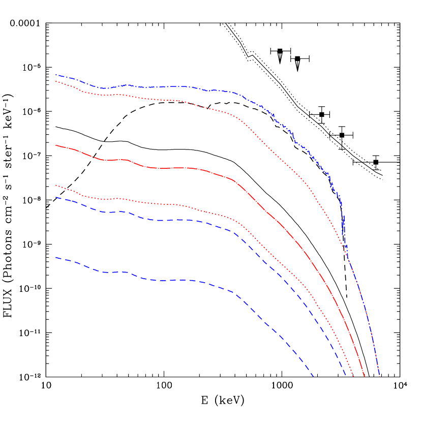
Figure 7.— The black line shows the addition of the contributions of NS–NS mergers in the KN and the remnant phase ( Figure 4 and Figure 5). The red–dotted lines corresponds to the upper and lower limits to the ejecta masses in that case. They are compared with that of SNe Ia (black dashed line), taken from Ruiz-Lapuente et al. (2016). Also shown (blue dot–dashed line) is the result of adding the KN contribution at its upper limit to the SN Ia contribution. Equally shown (blue dashed lines) are the contributions calculated for the upper and lower limits to the local KN rates of Abbott et al. (2020) and the combination of that upper limit with our highest estimate of the mass of the KN ejecta (red dot–long dashed line).

There has been another recent calculation of the gamma–ray emission from KNe (Li, 2019), where a semianalytic model of radiative transfer was introduced. In order to check the differences arising from two different treatments of the emission processes, we have also calculated the background using now the spectra shown in Fig. 14 of Li (2019) and corresponding to his standard case. The result is displayed in Figure 8, where it is compared with our own results for the emission in the KN phase of the ejecta (also in the standard case). We see that there is some difference, but not a very significant one.

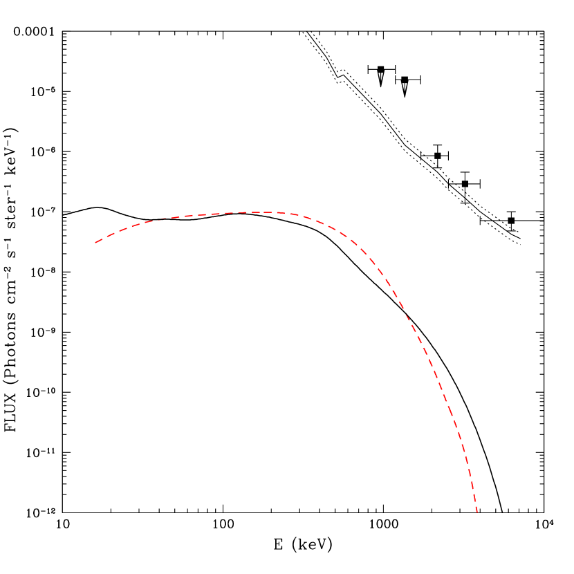
Figure 8.— Comparison of the contribution of NS–NS mergers to the cosmic gamma–ray background, in the KN phase, calculated from the emission spectra of Li (2019) (red slashed line), with that from the present work (continuous black line). The background observations are also shown, as in the previous Figures.

A further comparison is made in Figure 9, analogous to Figure 7, of the gamma–ray background calculated from Li (2019) and its upper and lower limits (estimated as in our case), with the contribution from SNe Ia. Also shown is the result of adding the KN contribution, taken at its upper limit, in this case, to the SNe Ia one.

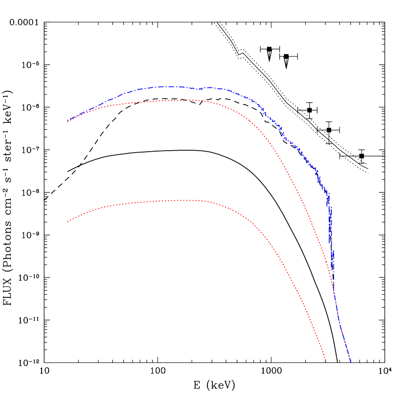
Figure 9.— Analogous to Figure 7, for the contribution of KNe to the cosmic gamma–ray background obtained from Li (2019) (continuous black line: standard case; dotted red lines, upper and lower limits). Also shown (blue dot–dashed line) is the result from adding together the upper limit of the KN contribution and that from SN Ia (shown by the black dashed line).

We must stress that our “reference” results shown in Figures 5–7 (and also the comparisons in Figures 8–9) correspond to the normalization of the KN rates to the upper limit to the local rate ($d<$ 40 Mpc) set by Yang et al. (2017), which is significantly higher than the upper limit set by Abbott et al. (2020) from the observations of GW170827 and GW190425, but still well within the uncertainty factor for the NS–NS merger rate indicated by Della Valle et al. (2018). In any case, as soon as the local merger rate estimates are refined, the Figures above need only to be rescaled to the new value of the rate. However, it seems improbable to reach the MeV background for any viable rate.

From the results obtained, we see that the KN contribution to the cosmic gamma–ray background (subjected to the previous caveat), although being non–negligible, appears minor as compared with that of SNe Ia. Only improbably high rates of NS–NS mergers and/or higher ejecta masses might change the situation. We must note, however, that even the contribution from SNe Ia falls short of explaining the observations in the MeV range, and some additional source has to be invoked. Flat–spectrum radio quasars (Ajello et al., 2009) (with a particular assumption about the location of the inverse–Compton peak in their spectra, due to the same electron population that emits the synchrotron bump), could explain the bulk of the background, though its slope in the MeV region does not really correspond to that of the data (see Figs. 15 and 16 of Ajello et al., 2009). Hidden cores of AGN could also originate MeV radiation. In that case, the MeV emission should correlate with the TeV neutrino background (Murase et al., 2019). This contribution to the gamma–ray background still needs to be fully calculated. The SN Ia contribution is quite substantial (see Fig. 13 in Ruiz-Lapuente et al., 2016). We see, in Figures 5– 8, that a KN contribution close to our upper limit or above would act analogously.

The question arises of the upper limit set by the observed abundances of r–process elements to the combination of NS–NS merger rate and r–process element yields in each merger event (Vangioni et al., 2016). Bovard et al. (2017) have addressed this point (see their Fig. 14). They adopt a simple model of Galactic evolution (see also Côté et al., 2017), where the yields from each event accumulate along the history of the Galaxy. It must be taken into account, however, that the KN ejecta move at velocities ${v_{dyn}\sim 0.2c}$ (dynamical component) and ${v_{wind}\sim 0.08c}$ (wind component). Such velocities are much higher that those of the SN ejecta and can allow escape from the Galaxy of a large fraction of the material, especially given that NS–NS mergers, as shown by the distribution of SGRBs in other galaxies (see Fong & Berger, 2013, for instance), occur far from the regions of star formation and even far away from the bulk of the stellar mass. That is due to the two successive kicks accompanying the formation of the two NSs (but see Piran & Shaviv, 2005; Beniamini & Piran, 2016). Given the very low densities of interstellar matter there, the ejecta should almost be expanding in a void and that, together with their high velocities, would made them leave the Galaxy (that would in no way affect their contribution to the background, though). Therefore, no robust upper limit can easily be derived to the combination of KN rate with the amount of ejected material per NS–NS merger.

Another point to be considered is that the gamma–ray emission from the radioactive elements created by the NS–NS mergers has a cut–off at $\sim$20 MeV. Although the location of the cutoff is much smeared when adding the contributions to the gamma–ray background at different redshifts, some feature might still show if the emission from KNe were dominant for $E_{\gamma}<$ 20 MeV. But the slope of the observed spectrum just flattens at $E\simeq$ 10 MeV (when going to higher energies), so not much can be concluded.

7. Summary and conclusions

Neutron star merger ejecta are emitters of gamma–rays in the MeV range, both in the kilonova (KN) phase of the ejection of r–process rich material and in the much longer remnant phase of the expansion. Based on recent calculations of the spectra of those emissions (KorBobkin et al., 2019; Li, 2019), we have estimated the contribution of NS–NS mergers to the cosmic gamma–ray background, which is significant in the range from 10 keV to a few MeV, just where there is a gap with no clear source (or sources) that can explain the observational data. We take into account the current, considerable discrepancies about the amount of material ejected in the mergers and also on the cosmic rates of these events.

We find that, within the current upper limits, the contribution of mergers falls short to explain the observed background, although its slope coincides with that of the observational data. At its upper limit, added to the contribution from SNe Ia (Ruiz-Lapuente et al., 2016) and from flat–spectrum radio quasars (Ajello et al., 2009), it would help to fit the data in the MeV region.

We have not included the contribution to the background from NS–BH mergers, for which there are no available calculations of the emitted gamma–ray spectra. In any case, their occurrence rate should be lower than that of NS–NS mergers, although the ejected masses might be larger.

Upcoming detections of gravitational–wave events and the observation of their electromagnetic counterparts should clarify the local merger rate and the amounts of r–process rich material ejected in the mergers. Eventually, the emitted gamma–rays from nearby events should be observed by some of the space missions planned for the near future. In particular, the enhanced ASTROGAM (e–ASTROGAM) space mission (Tatischeff et al., 2018; de Angelis et al., 2018) is conceived to study, with unprecedented sensitivity and resolution, the energy range from 300 keV to 3 GeV. Also, the All–Sky–ASTROGAM (Tatischeff et al., 2019), recently proposed as the “FAST” (F) mission of the European Space Agency, would explore the range from 100 keV to a few hundred MeV, with a very large field of view in this case. On the US side, NASA is considering a medium energy gamma–ray mission covering from 200 keV to 10 GeV, the All-sky Medium Energy Gamma-ray Observatory, AMEGO (McEnery et al., 2019). Both e–ASTROGRAM and AMEGO are planned to have a high sensitivity to measure the spectral energy distribution (SED) both in continuum and line emission with good spectral resolution and covering a wide field of view. They are planned to allow polarization studies as well. From all the above the spectral MeV range would be understood with high observational precision in the next decade and give an answer to the various candidate contributors.

References

- Abbott et al. (2017) Abbott, B. P., Abbott, R., Abbott, T. D., et al. 2017, Phys. Rev. Lett., 119, 161101
- Abbott et al. (2020) Abbott, B. P., Abbott, R., Abbott, T. D., et al. 2020, arXiv e-prints,arXiv: 2001.01761
- Ajello et al. (2009) Ajello, M., Costamante, L., Sambruna, R. M., et al. 2009, ApJ, 699, 603
- Ajello et al. (2015) Ajello, M., Gasparrini, D., Sánchez-Conde, M., et al. 2015, ApJ, 800, L27
- Ajello et al. (2019) Ajello, M., Inoue, Y., Bloser, P., et al. 2019, BAAS, 51, 290
- Arcavi et al. (2017) Arcavi, I., Hosseinzadeh, G., Howell, D. A., et al. 2017, Nature, 551, 64
- Barnes & Kasen (2013) Barnes, J., & Kasen, D. 2013, ApJ, 775, 18
- Bauswein et al. (2013) Bauswein, A., Goriely, S., & Janka, H.-T. 2013, ApJ, 773, 78
- Beniamini & Piran (2016) Beniamini, P., & Piran, T. 2016, MNRAS, 456, 4089
- Berger (2014) Berger, E. 2014, ARA&A, 52, 43
- Bovard et al. (2017) Bovard, L., Martin, D., Guercilena, F., et al. 2017, Phys. Rev. D, 96, 124005
- Côté et al. (2017) Côté, B., Belczynski, K., Fryer, C. L., et al. 2017, ApJ, 836, 230
- Côté et al. (2018) Côté, B., Fryer, C. L., Belczynski, K., et al. 2018, ApJ, 855, 99
- Coulter et al. (2017) Coulter, D. A., Foley, R. J., Kilpatrick, C. D., et al. 2017, Science, arXiv:1710.05452 [astro-ph.HE]
- Cucciati et al. (2012) Cucciati, O., Tresse, L., Ilbert, O., et al. 2012, A&A, 539, A31
- de Angelis et al. (2018) de Angelis, A., Tatischeff, V., Grenier, I. A., et al. 2018, Journal of High Energy Astrophysics, 19, 1
- Della Valle et al. (2018) Della Valle, M., Guetta, D., Cappellaro, E., et al. 2018, MNRAS, 481, 4355
- Desai et al. (2019) Desai, D., Metzger, B. D., & Foucart, F. 2019, MNRAS, 485, 4404
- Dessart et al. (2009) Dessart, L., Ott, C. D., Burrows, A., Rosswog, S., & Livne, E. 2009, ApJ, 690, 1681
- Di Mauro & Donato (2015) Di Mauro, M., & Donato, F. 2015, Phys. Rev. D, 91, 123001
- Dietrich & Ujevic (2017) Dietrich, T., & Ujevic, M. 2017, Classical and Quantum Gravity, 34, 105014
- Eichler et al. (1989) Eichler, D., Livio, M., Piran, T., & Schramm, D. N. 1989, Nature, 340, 126
- Evans et al. (2017) Evans, P. A., Cenko, S. B., Kennea, J. A., et al. 2017, Science, 358, 1565
- Fernández et al. (2015) Fernández, R., Kasen, D., Metzger, B. D., & Quataert, E. 2015, MNRAS, 446, 750
- Fong & Berger (2013) Fong, W., & Berger, E. 2013, ApJ, 776, 18
- Freiburghaus et al. (1999) Freiburghaus, C., Rosswog, S., & Thielemann, F.-K. 1999, ApJ, 525, L121
- Goldstein et al. (2017) Goldstein, A., Veres, P., Burns, E., et al. 2017, ApJ, 848, L14
- Goriely et al. (2011) Goriely, S., Bauswein, A., & Janka, H.-T. 2011, ApJ, 738, L32
- Grossman et al. (2014) Grossman, D., Korobkin, O., Rosswog, S., & Piran, T. 2014, MNRAS, 439, 757
- Holmbeck et al. (2019) Holmbeck, E. M., Sprouse, T. M., Mumpower, M. R., et al. 2019, ApJ, 870, 23
- Hotokezaka et al. (2013) Hotokezaka, K., Kiuchi, K., Kyutoku, K., et al. 2013, Phys. Rev. D, 87, 024001
- Hotokezaka et al. (2016) Hotokezaka, K., Wanajo, S., Tanaka, M., et al. 2016, MNRAS, 459, 35
- Hungerford et al. (2005) Hungerford, A. L., Fryer, C. L., & Rockefeller, G. 2005, ApJ, 635, 487
- Hungerford et al. (2003) Hungerford, A. L., Fryer, C. L., & Warren, M. S. 2003, ApJ, 594, 390
- Ji et al. (2019) Ji, A. P., Drout, M. R., & Hansen, T. T. 2019, ApJ, 882, 40
- Jin et al. (2016) Jin, Z.-P., Hotokezaka, K., Li, X., et al. 2016, Nature Communications, 7, 12898
- Kalogera et al. (2004a) Kalogera, V., Kim, C., Lorimer, D. R., et al. 2004a, ApJ, 614, L137
- Kalogera et al. (2004b) —. 2004b, ApJ, 601, L179
- Kappadath et al. (1996) Kappadath, S. C., Ryan, J., Bennett, K., et al. 1996, A&AS, 120, 619
- Kasen et al. (2013) Kasen, D., Badnell, N. R., & Barnes, J. 2013, ApJ, 774, 25
- Kasliwal et al. (2017) Kasliwal, M. M., Nakar, E., Singer, L. P., et al. 2017, Science, 358, 1559
- Kim et al. (2015) Kim, C., Perera, B. B. P., & McLaughlin, M. A. 2015, MNRAS, 448, 928
- Korobkin et al. (2012) Korobkin, O., Rosswog, S., Arcones, A., & Winteler, C. 2012, MNRAS, 426, 1940
- KorBobkin et al. (2019) Korobkin, O., Hungerford, A. M., Fryer, C. L., et al. 2019, arXiv e-prints, arXiv:1905.05089
- Kulkarni (2005) Kulkarni, S. R. 2005, arXiv e-prints, astro
- Lacki et al. (2014) Lacki, B. C., Horiuchi, S., & Beacom, J. F. 2014, ApJ, 786, 40
- Lattimer & Schramm (1974) Lattimer, J. M., & Schramm, D. N. 1974, ApJ, 192, L145
- Li (2019) Li, L.-X. 2019, ApJ, 872, 19
- Li & Paczyński (1998) Li, L.-X., & Paczyński, B. 1998, ApJ, 507, L59
- Lippuner & Roberts (2015) Lippuner, J., & Roberts, L. F. 2015, ApJ, 815, 82
- Lipunov et al. (2017) Lipunov, V. M., Gorbovskoy, E., Kornilov, V. G., et al. 2017, ApJ, 850, L1
- Madau et al. (1994) Madau, P., Ghisellini, G., & Fabian, A. C. 1994, MNRAS, 270, L17
- McCully et al. (2017) McCully, C., Hiramatsu, D., Howell, D. A., et al. 2017, ApJ, 848, L32
- McEnery et al. (2019) McEnery, J. & et al. 2019, AMEGO White Paper; arXiv e-prints, arXiv:1907.07558
- Metzger (2019) Metzger, B. D. 2019, Living Reviews in Relativity, 23, 1
- Metzger & Berger (2012) Metzger, B. D., & Berger, E. 2012, ApJ, 746, 48
- Metzger et al. (2010) Metzger, B. D., Martínez-Pinedo, G., Darbha, S., et al. 2010, MNRAS, 406, 2650
- Miller et al. (2019) Miller, J. M., Ryan, B. R., Dolence, J. C., et al. 2019, Phys. Rev. D, 100, 023008
- Murase et al. (2019) Murase, K., Kimura, S.S., Mészáros, P. 2019, arXiv e-prints,arXiv: 1904.04226
- Nakar (2007) Nakar, E. 2007, Phys. Rep., 442, 166
- Perego et al. (2014) Perego, A., Rosswog, S., Cabezón, R. M., et al. 2014, MNRAS, 443, 3134
- Pian et al. (2017) Pian, E., D’Avanzo, P., Benetti, S., et al. 2017, Nature, 551, 67
- Piran et al. (2014) Piran, T., Korobkin, O., & Rosswog, S. 2014, arXiv e-prints, arXiv:1401.2166
- Piran & Shaviv (2005) Piran, T., & Shaviv, N. J. 2005, Phys. Rev. Lett., 94, 051102
- Planck Collaboration & et al. (2018) Planck Collaboration, & et al. 2018, arXiv e-prints, arXiv:1807.06209
- Pozanenko et al. (2019) Pozanenko, A.S. Minaev, P.Y., Grevenev, S.A., & Chelovekov, I.V. 2019, arXiv e–prints, arXiv:1912.13112
- Radice et al. (2016) Radice, D., Galeazzi, F., Lippuner, J., et al. 2016, MNRAS, 460, 3255
- Rosswog et al. (2018) Rosswog, S., Sollerman, J., Feindt, U., et al. 2018, A&A, 615, A132
- Ruiz-Lapuente et al. (2016) Ruiz-Lapuente, P., The, L.-S., Hartmann, D. H., et al. 2016, ApJ, 820, 142
- Smartt et al. (2017) Smartt, S. J., Chen, T.-W., Jerkstrand, A., et al. 2017, Nature, 551, 75
- Soares-Santos et al. (2017) Soares-Santos, M., Holz, D. E., Annis, J., et al. 2017, ApJ, 848, L16
- Tanvir et al. (2013) Tanvir, N. R., Levan, A. J., Fruchter, A. S., et al. 2013, Nature, 500, 547
- Tanvir et al. (2017) Tanvir, N. R., Levan, A. J., González-Fernández, C., et al. 2017, ApJ, 848, L27
- Tatischeff et al. (2018) Tatischeff, V., De Angelis, A., Tavani, M., et al. 2018, in Society of Photo-Optical Instrumentation Engineers (SPIE) Conference Series, Vol. 10699, Proc. SPIE, 106992J
- Tatischeff et al. (2019) Tatischeff, V., De Angelis, A., Tavani, M., et al. 2019, arXiv e-prints, arXiv:1905.07806
- Ueda et al. (2003) Ueda, Y., Akiyama, M., Ohta, K., & Miyaji, T. 2003, ApJ, 598, 886
- Valenti et al. (2017) Valenti, S., David, Sand, J., et al. 2017, ApJ, 848, L24
- Vangioni et al. (2016) Vangioni, E., Goriely, S., Daigne, F., Francois, P., & Belczynski, K. 2016, MNRAS, 455,17
- Wanajo et al. (2014) Wanajo, S., Sekiguchi, Y., Nishimura, N., et al. 2014, ApJ, 789, L39
- Wanderman & Piran (2015) Wanderman, D., & Piran, T. 2015, MNRAS, 448, 3026
- Watanabe et al. (1999) Watanabe, K., Leising, M., Share, G., & Kinzer, R. 1999, in AAS/High Energy Astrophysics Division #4, AAS/High Energy Astrophysics Division, 06.01
- Weidenspointner (1999) Weidenspointner, G. 1999, Dissertation, Technische Universität München, München
- Weidenspointner et al. (2000) Weidenspointner, G., Varendorff, M., Oberlack, U., P. S., et al. 2000, in AIP Conference Proceedings, 581
- Winteler et al. (2012) Winteler, C., Käppeli, R., Perego, A., et al. 2012, ApJ, 750, L22
- Wollaeger et al. (2018) Wollaeger, R. T., Korobkin, O., Fontes, C. J., et al. 2018, MNRAS, 478, 3298
- Woosley et al. (1994) Woosley, S. E., Wilson, J. R., Mathews, G. J., Hoffman, R. D., & Meyer, B. S. 1994, ApJ, 433, 229
- Yang et al. (2017) Yang, S., Valenti, S., Cappellaro, E., et al. 2017, ApJ, 851, L48