e1e-mail: tcsorgo@cern.ch
\thankstexte2e-mail: novak.tamas@uni-mate.hu
Before February 1, 2021:
Szent István University, Károly Róbert Campus
\thankstexte3e-mail: roman.pasechnik@thep.lu.se
\thankstexte4e-mail: ster.andras@wigner.hu
\thankstexte5e-mail: istvan.szanyi@cern.ch
Evidence of Odderon-exchange from scaling properties
of elastic scattering at TeV energies
Abstract
We study the scaling properties of the differential cross section of elastic proton-proton () and proton-antiproton () collisions at high energies. We introduce a new scaling function, that scales – within the experimental errors – all the ISR data on elastic scattering from to GeV to the same universal curve. We explore the scaling properties of the differential cross-sections of the elastic and collisions in a limited TeV energy range. Rescaling the TOTEM data from TeV to and TeV, and comparing it to D0 data at TeV, our results provide an evidence for a -channel Odderon exchange at TeV energies, with a significance of at least 6.26. We complete this work with a model-dependent evaluation of the domain of validity of the new scaling and its violations. We find that the scaling is valid, model dependently, within GeV TeV, with a range gradually narrowing with decreasing colliding energies.
1 Introduction
One of the most important and critical tests of quantum chromodynamics (QCD) in the infrared regime is provided by the ongoing studies of elastic differential hadron-hadron scattering cross section at various energies and momentum transfers. The characteristics of the elastic amplitude, its both real and imaginary parts, carry a plenty of information about the inner proton structure, the proton profile in the impact parameter space and its energy dependence, as well as about the properties of QCD exchange interaction at low momentum transfers.
The first and most precise measurement of the total, elastic and differential cross sections of elastic collisions, together with the -parameter, has recently been performed by the TOTEM Collaboration at the Large Hadron Collider (LHC) at CERN at the highest energy frontier of TeV (for the corresponding recent TOTEM publications, see Refs. Antchev:2017dia ; Antchev:2017yns ; Antchev:2018edk ; Antchev:2018rec ). A correct theoretical interpretation of the LHC data, together with the lower-energy Tevatron and ISR data, is a subject of intense debates and ongoing research development in the literature, see e.g. Refs. Samokhin:2017kde ; Khoze:2018kna . Among the important recent advances, data by the TOTEM Collaboration Antchev:2018rec for the first time have indicated the presence of an odd-under-crossing (or C-odd) contribution to the elastic scattering amplitude known as the Odderon Lukaszuk:1973nt . In particular, a comparison of the differential cross-section of elastic proton-proton () scattering obtained by the TOTEM Collaboration at TeV with D0 results on elastic proton-antiproton () scattering at 1.96 TeV Abazov:2012qb indicates important qualitative differences that can be attributed to the Odderon effect Csorgo:2018uyp ; Antchev:2018rec . In the more rigorous language of QCD, an Odderon exchange is usually associated with a quarkless odd-gluon (e.g. three-gluon, to the lowest order) bound state such as a vector glueball, and a vast literature is devoted to theoretical understanding of its implications. An increase of the total cross section, , associated with a decrease of the real-to-imaginary ratio, , with energy, first identified at TeV Antchev:2017dia ; Antchev:2017yns , also indicated a possible Odderon effect.
The TOTEM measurements have recently triggered intense theoretical studies in the literature. In particular, the Phillips-Barger parameterisation of the elastic amplitude has been found to describe the recent data in Refs. Ster:2015esa ; Goncalves:2018nsp . Several other Regge parameterisations have also been found to describe the LHC data reasonably well (see e.g. Refs. Khoze:2017swe ; Khoze:2018kna ; Selyugin:2018uob ), while the Pomeron dominance has been explored in a generic Regge theory set-up in Refs. Broilo:2018els ; Broilo:2018qqs . In Ref. Samokhin:2017kde , a new feature of the second diffractive cone in the differential cross-section of elastic scattering at large and has been identified arguing about the existence of two stationary points in at the LHC energies and relating those to the two-scale structure of protons at these energies. Remarkably, this rules out the dominance of perturbative exchanges of a few non-interacting gluons pointing towards a core-like proton substructure found also in the framework of the so-called Lévy imaging technique in Refs. Csorgo:2018uyp ; Csorgo:2019egs . For a thorough discussion of general properties of the -dependence of in the light of the TOTEM data and its connections to the growing energy dependence of the elastic-to-total cross–sections ratio, see Ref. Troshin:2018ihb . A number of studies based upon a QCD-based analysis of the Odderon signatures considering the non-linear QCD evolution have also been triggered recently (see e.g. Refs. Gotsman:2018buo ; Gotsman:2020mkd ; Hagiwara:2020mqb ; Contreras:2020lrh ).
Important statements about the maximal nature of the Odderon effect were made in Refs. Martynov:2018nyb ; Martynov:2018sga ; Shabelski:2018jfq ; Khoze:2018kna but apparently these studies still lack a rigorous statistical significance analysis. Although the -dependence of both and is consistent with an Odderon effect, this indication is not a unique Odderon signal as the same effect can also be attributed to the secondary Reggeon effects Gotsman:2018buo , reinforcing the elusiveness of the Odderon. As it was argued in Ref. Pancheri any conclusions about the magnitude of the Odderon effects based upon the measurement alone have to be made with special care due to a zero in the real part of the elastic amplitude at very small , as the latter can affect the Coulomb-Nuclear Interference (CNI) region at high energies.
In earlier studies of Refs. Csorgo:2018ruk ; Csorgo:2019rsr , the Odderon signatures have been identified and qualitatively described in a model-independent way using the power of the Lévy imaging technique Csorgo:2018uyp . One of such signatures concern the presence of a dip-and-bump structure in the differential cross section of elastic collisions and the lack of such a structure in elastic collisions. The latter effectively emerges in the -dependence of the elastic slope , that crosses zero for elastic collisions and remains non-negative for all values of in elastic collisions. Besides, Ref. Csorgo:2018uyp noted that the position of the node of the nuclear phase , as reconstructed with the help of the Lévy expansion method, is characteristically and qualitatively different for elastic from collisions, thus, indicating the Odderon exchange. In addition, the presence of a smaller substructure of the proton has been revealed in the data that is imprinted in the behaviour of the -dependent elastic slope , apparent at large values of . In particular, in Refs. Csorgo:2018uyp ; Csorgo:2018ruk ; Csorgo:2019rsr ; Csorgo:2019egs two substructures of two distinct sizes have been identified in the low (a few tens of GeV) and high (a few TeV) energy domains, respectively. Besides, a new statistically significant feature in the -dependent shadow (or inelasticity) profile has been found at the maximal available energy TeV and represents a long-debated hollowness, or “black-ring” effect that emerges instead of the conventionally anticipated “black-disk” regime Csorgo:2018ruk ; Csorgo:2019egs .
In this paper, in order to further unveil the important characteristics of elastic hadron-hadron scattering we study the scaling properties of the existing data sets available from the ISR and Tevatron colliders as well as those provided by the TOTEM Collaboration in a TeV energy range Antchev:2013gaa ; Antchev:2017dia ; Antchev:2017yns ; Antchev:2018edk ; Antchev:2018rec . We investigate a generic scaling behavior of elastic differential proton-(anti)proton scattering cross section, with the goal of transforming out the trivial colliding energy dependent variation of the key observables like that of the total and elastic cross-sections and , the elastic slope and the real-to-imaginary ratio . We search successfully for a universal scaling function and the associated data-collapsing behaviour that is valid not only in the low- domain, but also in the dip-and-bump region. We discuss the physics implications of such a scaling behaviour and explore its consequences for understanding of the Odderon effect as well as the high-energy behaviour of the proton structure.
The paper is organised as follows. In section 2, we recapitulate the formalism that is utilized for evaluation of the observables of elastic proton-(anti)proton scattering in the TeV energy range. In section 3, we connect this formalism to a more general strategy of the experimental Odderon search, namely, to the search for a crossing-odd component in the differential cross-section of elastic proton-(anti)proton scattering. In section 4, we study some of the scaling functions of elastic scattering already existing in the literature as well as propose a new scaling function denoted as that is readily measurable in and collisions. In particular, in subsection 4.3 we introduce a new scaling function for the diffractive cone or low values of the square of the four-momentum () region. We generalize this scaling function for larger values of in subsection 4.4 and present a first test of the scaling in the ISR energy range of 23.5 – 62.5 GeV in the same subsection. Subsequently, in section 5 we extend these studies to the TeV (Tevatron and LHC) energy range, where the possible residual effects of Reggeon exchange are expected to be below the scale of the experimental errors Broniowski:2018xbg . In section 6, we present a method of how to quantify the significance of our findings, giving the formulas that are used to evaluate , confidence level (CL), and significance in terms of the standard deviation, . In section 7, we discuss how to employ the newly found scaling behavior of the differential cross-section to extrapolate the differential cross-sections of elastic scattering within the domain of the validity of the new scaling. Let us note, that this method of comparing differential cross-sections is a possible strategy for the Odderon search. However, as we detail later, the overall normalization uncertainties are large and reduce the statistical significance of these kind of results: practically it is a better strategy to compare scaling functions, evaluated from the differential cross-sections in such a way, that the overall normalization constants (including their large errors) cancel. In section 8, we present further, more detailed results of our studies with the help of and compare such a scaling function for differential cross-sections at the LHC energies with the scaling function at the Tevatron energy. In section 9 we evaluate the significance of the Odderon-effect, and find that it is at least a 6.26-significant effect, taking into account also the improvements detailed in A. Subsequently, we present several cross-checks in section 10 and discuss the main results and its implications in section 11. Finally, we summarize and conclude our work in section 12.
This manuscript is completed with several Appendices that highlight various aspects of this analysis. A details the robustness and symmetry properties of the definition and provides the final Odderon significance of at least from a model-independent comparison of the scaling functions of already published data. In B we discuss the model-independent properties of the Pomeron and Odderon exchanges at the TeV energy scale, under the condition that this energy is sufficiently large: as the effects from the exchange of known hadronic resonances decreases as an inverse power of , at large enough energies Pomeron and Odderon exchanges can be identified with the crossing-even and the crossing-odd contributions to the elastic scattering, respectively. We demonstrate here that -matrix unitarity constrains the possible form of the impact-parameter dependence of the Pomeron and Odderon amplitudes. In C, we discuss model-dependent properties of the Pomeron and Odderon exchanges at the TeV energy scale and derive, how the scaling emerges within a specific model, defined in Ref. Nemes:2015iia . This model is one of the possible models in the class considered in B. We evaluate the experimentally observable consequences of the scaling in D, where we estimate the domain of validity of the scaling also in a model-dependent manner, based on Ref. Nemes:2015iia . Finally, in E we cross-check the stability and robustness of the Odderon signal for the variation of the -range, the domain or support in where the signal is determined. We also identify here a minimal set of only 8 out of 17 D0 datapoints, close to the diffractive interference region, that alone carry an at least 5 Odderon signal, when compared to the TOTEM datapoints in the same region.
2 Formalism
For the sake of completeness and clarity, let us start first with recapitulating the connection between the scattering amplitude and the key observables of elastic scattering, following the conventions of Refs. Bialas:2006qf ; Nemes:2012cp ; CsorgO:2013kua ; Nemes:2015iia .
The Mandelstam variables and are defined as usual , for an elastic scattering of particles and with incoming four-momenta and , and outgoing four-momenta and , respectively.
The elastic cross-section is given as an integral of the differential cross-section of elastic scattering:
| (1) |
The elastic differential cross section is
| (2) |
The -dependent slope parameter is defined as
| (3) |
and in the experimentally accessible low- region this function is frequently assumed or found within errors to be a constant. In this case, a -independent slope parameter is introduced as
| (4) |
where the limit is taken within the experimentally probed region. Actually, experimentally the optical point can only be approached by extrapolations from the measurements in various kinematically accessible regions that depend on the optics and various settings of the particle accelerators and colliding beams.
According to the optical theorem, the total cross section is also found by a similar extrapolation. Its value is given by
| (5) |
while the inelastic cross-section is defined by
| (6) |
The ratio of the real to imaginary parts of the elastic amplitude is found as
| (7) |
and its measured value at reads
| (8) |
Here, the limit is taken typically as an extrapolation in dedicated differential cross section measurements at very low , where the parameter can be measured using various CNI methods. The differential cross section at the optical point is thus represented as
| (9) |
In the impact-parameter -space, we have the following relations:
| (10) | |||||
| (11) |
This Fourier-transformed elastic amplitude can be represented in the eikonal form
| (12) |
where is the so-called opacity function (known also as the eikonal function), which is complex in general. The shadow profile function is then defined as
| (13) |
For clarity, let us note that other conventions are also used in the literature and for example the shadow profile is also referred to as the inelasticity profile function since it corresponds to the probability distribution of inelastic proton-proton collisions in the impact parameter with . When the real part of the scattering amplitude is neglected, is frequently denoted as , see for example Refs. Petrov:2018rbi ; Dremin:2013qua ; Dremin:2014spa ; Dremin:2018urc ; Dremin:2019tgm .
3 Looking for Odderon effects in the differential cross-section of elastic scattering
As noted in Refs. Jenkovszky:2011hu ; Ster:2015esa , the only direct way to see the Odderon is by comparing the particle and antiparticle scattering at sufficiently high energies provided that the high-energy or elastic scattering amplitude is a sum or a difference of even and odd C-parity contributions, respectively,
| (14) | |||||
| (15) | |||||
| (16) | |||||
| (17) |
Here, the even-under-crossing part consists of the Pomeron and the Reggeon trajectories, while the odd-under-crossing part contains the Odderon and a contribution from the Reggeon .
At sufficiently high collision energies , the relative contributions from secondary Regge trajectories are suppressed since they decay as negative powers of . In Ref. Ster:2015esa , the authors argued that the LHC energy scale is already sufficiently large to suppress the Reggeon contributions, and they presented the -dependent contributions of an Odderon exchange to the differential and total cross-sections at typical LHC energies. More recently, this observation was confirmed in Ref. Broniowski:2018xbg , suggesting that indeed the relative contribution of the Reggeon trajectories is well below the experimental precision in elastic scattering in the TeV energy range. The analysis of Ref. Ster:2015esa relies on a model-dependent, phenomenological picture formulated in the framework of the Phillips-Barger model Phillips:1974vt and is focused primarily on fitting the dip region of elastic scattering, but without a detailed analysis of the tail and cone regions. In Ref. Broniowski:2018xbg , a phenomenological Reggeon + Pomeron + Odderon exchange model is employed to study, in particular, the possible hollowness effect in the high-energy elastic collisions. A similar study of the Philips-Barger model was performed in Ref. Goncalves:2018nsp using the most recent TOTEM data on elastic scattering. Similarly, Ref. Lebiedowicz:2018eui has also argued that the currently highest LHC energy of 13 TeV is sufficiently high to observe the Odderon effect.
In this paper, we follow Refs. Ster:2015esa ; Broniowski:2018xbg ; Lebiedowicz:2018eui and assume that the Reggeon contributions to the elastic scattering amplitudes for 1.96 TeV and at higher energies are negligibly small. We search for an odd-under-crossing contribution to the scattering amplitude, in a model independent way, and find that such a non-vanishing contribution is present at a TeV scale that is recognised as an Odderon effect. The vanishing nature of the Reggeon contributions offers a direct way of extracting the Odderon as well as the Pomeron contributions, and , respectively, from the elastic and scattering data at sufficiently high colliding energies as follows
| (18) | |||||
| (19) |
These kind of studies rely on the extrapolation of the fitted model parameters of and reactions to an exactly the same energy, given that the elastic and scattering data have not been measured at the same (or close enough) energies in the TeV region so far. Another problem is a lack of precision data at the low- and high-, primarily, in collisions. Recently, the TOTEM Collaboration noted in Ref. Antchev:2018rec that “Under the condition that the effects due to the energy difference between TOTEM and D0 can be neglected, the result" (namely the differential cross-section measured by TOTEM at TeV) "provides evidence for a colourless 3-gluon bound state exchange in the t-channel of the proton-proton elastic scattering". In other words, if the effects due to the energy difference between TOTEM and D0 measurements can be neglected, the direct comparison of the differential cross section of elastic scattering at with that of scattering at TeV provides a conditional evidence for a colourless three-gluon state exchange in the -channel.
In this paper, we show that the conditional evidence stated by TOTEM can be turned to an unconditional evidence, i.e. a discovery of the Odderon, by closing the energy gap as much as possible at present, without a direct measurement, based on a re-analysis of already published TOTEM and D0 data.
Our main result, an at least 6.26 Odderon effect, is obtained by taking the data at a face value as given in published sources, without any attempt to extrapolate them with a help of a model, or using phenomenological, -dependent parameters and extrapolating them towards their unmeasured values (in unexplored energy domains). Nevertheless, we have tested what happens if one employs this kind of model as detailed in a different manuscript, see Ref. Csorgo:2020wmw . These model-dependent results lead to a higher than 7.08 combined significance for the Odderon effect, based on the results of C. The experimentally observable signs of the newly found scaling are detailed in D, where we also determine the model-dependent domain of validity of this new scaling and find that this domain of validity is model-dependently, but sufficiently large so that the Odderon signal remains well above the discovery threshold of a 5 effect, as detailed in E. As the 7.08 combined significance is based only on model-dependent results, evaluated and combined at two energies, and TeV (detailed in both C and E), we find that the model-independent approach, summarized in the body of this manuscript and detailed in A and B, provides a more conservative, 6.26 estimate for the Odderon significance.
Our main result is based on the validity of a new kind of scaling relation, called as the -scaling. We test this scaling on the experimental data and show their data-collapsing behaviour in a limited energy range. We demonstrate that such a data-collapsing behaviour can be used to close the small energy gap between the highest-energy elastic collisions, TeV and the lowest-energy elastic collisions at the LHC where the public data are available, TeV. We investigate the stability of this result on the -range or the domain of validity of the scaling in E. We find that the result is extremely stable for the removal of data points at the beginning or at the end of the acceptance of the D0 experiment. Namely, 9 out of the 17 D0 data points can be removed without decreasing the significance of the Odderon signal below the 5 discovery threshold.
We look for the even-under-crossing and odd-under-crossing contributions by comparing the scaling functions of and collisions in the TeV energy range. In other words, we look for and find a robust Odderon signature in the difference of the scaling functions of the elastic differential cross-section between and collisions. We thus discuss the Odderon features that can be extracted in a model-independent manner by directly comparing the corresponding data sets to one another.
Let us start with three general remarks as direct consequences of Eqs. (18,19):
-
•
If the Odderon exchange effect is negligibly small (within errors, equal to zero) or if it does not interfere with that of the Pomeron at a given energy, then the differential cross sections of the elastic and scattering have to be equal:
(20) -
•
If the differential cross sections of elastic and collisions are equal within the experimental errors, this does not imply that the Odderon contribution has to be equal to zero. Indeed, the equality of cross sections does not require the equality of complex amplitudes:
(21) -
•
If the differential cross sections differ from that of scattering at the same value of in a TeV energy domain, then the Odderon contribution to the scattering amplitude cannot be equal to zero, i.e.
(22)
Such a difference is thus a clear-cut signal for the Odderon-exchange, if the differential cross sections were measured at exactly the same energies. However, currently such data are lacking in the TeV energy range. Our research strategy in this paper is to scale out the known -dependencies of the differential cross section by scaling out its dependencies on , , and functions. The residual scaling functions will be compared for the and elastic scattering to see if any difference remains.
4 Possible scaling relations at low values of
In this section, let us first investigate the scaling properties of the experimental data based on a simple Gaussian model elaborating on the discussion presented in Ref. Csorgo:2019fbf . The motivation for this investigation is that we would like to work out a scaling law that works at least in the simplest, exponential diffractive cone approximation, and scales out the trivial -dependencies of , , , and . Based on the results of such a frequently used exponential approximation, we gain some intuition and experience on how to generalize such scaling laws for realistic non-exponential differential cross sections.
Experimentally, the low- part of the measured distribution is usually approximated with an exponential,
| (23) |
where it is explicitly indicated that both the normalization parameter and the slope parameter are the functions of the center-of-mass energy squared . If the data deviate from such an exponential shape, that can be described if one allows for a -dependence of the slope parameter as defined in Eq. (3). For simplicity, we would like to scale out the energy dependence of the elastic slope from the differential cross section of elastic scattering, together with the energy dependence of the elastic and total cross sections, and , as detailed below. For this purpose, let us follow the lines of a similar derivation in Refs. Broniowski:2018xbg ; Csorgo:2019fbf .
It is clear that Eq. (23) corresponds to an exponential “diffractive cone” approximation, that may be valid in the low- domain only. This equation corresponds to the so called “Grey Gaussian” approximation that suggests a relationship between the nuclear slope parameter , the real-to-imaginary ratio , the total cross section , and the elastic cross section as follows Block:2006hy ; Fagundes:2011hv ; Broniowski:2018xbg :
| (24) | |||||
| (25) |
Such relations for and parameters in terms of the elastic and total cross sections are particularly useful when studying the shadow profile function as detailed below. The above relationships, in a slightly modified form, have been utilized by TOTEM to measure the total cross section at 2.76, 7, 8 and 13 TeV in Refs. Nemes:2017gut ; Antchev:2013iaa ; Antchev:2013paa ; Antchev:2017dia , using the luminosity independent method. In what follows, we do not suppress the -dependence of the observables, i.e. , .
4.1 Scaling properties of the shadow profiles
In the exponential approximation given by Eqs. (23,24,25), the shadow profile function introduced in Eq. (13) has a remarkable and very interesting scaling behaviour, as anticipated in Ref. Broniowski:2018xbg :
| (26) | |||||
| (27) |
Thus, the shadow profile at the center, reads as
| (28) |
which cannot become maximally absorptive (or black), i.e. is not reached at those colliding energies, where is not negligibly small. The maximal absorption corresponds to , which is rather independent of the detailed -dependent shape of the inelastic collisions Broniowski:2018xbg . It is achieved when of Eq. (27) approaches the value . Thus, at such a threshold, we have the following critical value of the ratio
| (29) |
As for the existing measurements and seems to decrease with increasing energies at least in the 8 TeV region, the critical value of the elastic-to-total cross section ratio (29) corresponds to, roughly, %. Evaluating the second derivative of at , one may also observe that it changes sign from a negative to a positive one exactly at the same threshold given by Eq. (29). Such a change of sign can be interpreted as an onset of the hollowness effect Broniowski:2018xbg . The investigation of such a hollowness at is a hotly debated topic in the literature. For early papers on this fundamental feature of scattering at the LHC and asymptotic energies, see Refs. Troshin:2007fq ; Fagundes:2011hv ; Dremin:2013qua ; Alkin:2014rfa ; Troshin:2014rva ; Dremin:2014spa ; Anisovich:2014wha , as well as Refs. RuizArriola:2016ihz ; Troshin:2016frs ; Albacete:2016pmp ; Broniowski:2017aaf ; Broniowski:2017rhz ; Troshin:2017ucy ; Dremin:2018orv ; Campos:2018tsb ; Dremin:2018urc ; Broniowski:2018xbg ; Petrov:2018rbi ; Dremin:2019tgm for more recent theoretical discussions.
As pointed out in Ref. Csorgo:2019fbf , the threshold (29), within errors, is reached approximately already at TeV. The threshold behavior saturates somewhere between 2.76 and 7 TeV and a transition may happen around the threshold energy of TeV. The elastic-to-total cross section ratio becomes significantly larger than the threshold value at TeV. As a result, the shadow profile function of the proton undergoes a qualitative change in the region of TeV energies. At high energies, with , the hollowness effect may become a generic property of the impact parameter distribution of inelastic scatterings. However, the expansion at low impact parameters corresponds to the large- region of elastic scattering, where the diffractive cone approximation of Eqs. (23,24,25) technically breaks down, and more refined studies are necessary (see below). For the most recent, significant and model-independent analysis of the hollowness effect at the LHC and its extraction directly from the TOTEM data, see Ref. Csorgo:2019egs .
4.2 Scaling functions for testing the black-disc limit
When discussing the scaling properties of the differential cross section of elastic scattering, let us mention that various scaling laws have been proposed to describe certain features and data-collapsing behaviour of elastic proton-proton scattering already in the 1970s. One of the early proposals was the so called geometric scaling property of the inelastic overlap function DiasDeDeus:1987njz ; Buras:1973km . The concept of geometric scaling was based on a negligibly small ratio of the real-to-imaginary parts of the scattering amplitude at , and resulted in an -independent ratio of the elastic-to-total cross-sections, , while at the LHC energies, is not negligibly small and the elastic-to-total cross section ratio is a strongly rising function of . Here, we just note about the geometric scaling as one of the earliest proposals to have a data-collapsing behavior in elastic scattering, but we look in detail for other kind of scaling laws that are more in harmony and consistency with the recent LHC measurements Csorgo:2019fbf .
Let us first detail the following two dimensionless scaling functions proposed in Ref. CsorgO:2013kua and denoted as and in what follows. These scaling functions were introduced in order to cross-check if elastic collisions at the LHC energies approach the so-called black-disc limit, expected at ultra-high energies, or not. In a strong sense, the black disc limit corresponds to the shadow profile that results in , independently of the black disc radius . This limit is clearly not yet approached at LHC energies, but in a weak sense, a black-disc limit is considered to be reached also if the shadow profile function at reaches unity, i.e. , corresponding to black disc scattering at zero impact parameter. This kind of black disc scattering might have been approached at TeV LHC energy Nemes:2015iia .
The first scaling function of the differential cross-section is defined as follows:
| (30) | |||||
| (31) |
In the diffractive cone approximation, the -dependence in does not cancel, but it can be approximately written as
| (32) | |||||
| (33) |
This result clearly indicates that in the diffractive cone, generally the scaling is violated by energy-dependent factors, while in the black-disc limit of elastic scattering, corresponding to and , the scaling becomes valid as detailed and discussed in Ref. CsorgO:2013kua . Indeed, the aim to introduce the scaling function was to clarify that even at the highest LHC energies we do not reach the black-disk limit (in the strong sense). As discussed in the previous section, the deviations from the black-disc limit might be due to the effects of the real part and the hollowness, i.e. reaching a black-ring limit instead of a black-disc one at the top LHC energies.
Since in the scaling function the position of the diffractive minimum (dip) remains -dependent, yet another scaling function denoted as was proposed to transform out such -dependence of the dip. This function was introduced also in Ref. CsorgO:2013kua as follows:
| (34) | |||||
| (35) |
In principle, all black-disc scatterings, regardless of the value of the total cross section, should show a data-collapsing behaviour to the same scaling function. As observed in Ref. CsorgO:2013kua , such an asymptotic form of the scaling function is somewhat better approached at the LHC energies as compared to the lower ISR energies but still not reproduced it exactly. This is one of the key indications the black-disc limit in the elastic scattering is not achieved at the LHC, up to TeV. This may have several other important implications. For example, this result indicates that in simulations of relativistic heavy-ion collisions at the LHC energies, more realistic profile functions have to be used to describe the impact parameter dependence of the inelastic collisions: a simple gray or black-disc approximation for the inelastic interactions neglects the key features of elastic collisions at the TeV energy scales.
One advantage of the scaling variables and mentioned above is that they are dimensionless. Numerically, corresponds to the function if the scaling variable is rescaled to . As indicated in Fig. 23 of Ref. CsorgO:2013kua , indeed the main difference between and is that the diffractive minimum is rescaled in to the position, so has less evolution with as compared to . However, as it is clear from the above discussion, the function
| (36) | |||||
| (37) |
is well-defined only for elastic scattering, where a unique dip structure is observed experimentally.
Even the dip region is not always measurable in reactions if the experimental acceptance is limited to the cone region, which is a sufficient condition for the total cross section measurements. If the acceptance was not large enough in to observe the diffractive minimum, or, in the case when the diffractive minimum did not clearly exist, then neither the nor the scaling functions would be usable. So, the major disadvantage of these scaling functions for extracting the Odderon signatures from the data is that in collisions no significant diffractive minimum is found by the D0 collaboration at 1.96 TeV Abazov:2012qb . Besides, even if variable were defined, the above expressions indicate, in agreement with Fig. 23 of Ref. CsorgO:2013kua , that the scaling function has a non-trivial energy-dependent evolution in the cone () region. Due to these reasons, variables and are not appropriate scaling variables for a scale-invariant analysis of the crossing-symmetry violations at high energies.
Having recapitulated the considerations in Ref. Csorgo:2019fbf , with an emphasis on the -dependence of the parameters, let us now consider, how these -dependencies can be scaled out at low values of , where the diffraction cone approximation is valid, by evaluating the scaling properties of the experimental data on the differential elastic and cross sections. For this purpose, let us look into the scaling properties of the differential cross sections and their implications related to the Odderon discovery in a new way.
4.3 A new scaling function for the elastic cone
In the elastic cone region, all the and differential cross sections can be rescaled to a straight line in a linear-logarithmic plot, when the horizontal axis is scaled by the slope parameter to while the vertical axis is simultaneously rescaled by , namely,
| (38) |
This representation, in the diffractive cone, scales out the -dependencies of the total and elastic cross section, and , and also that of the slope parameter, . As a function of the scaling variable , it will correspond to the plot of i.e. a straight line with slope on a linear-logarithmic plot. It is well-known that the elastic scattering is only approximately exponential in the diffractive cone, but by scaling out this exponential feature one may more clearly see the scaling violations on this simple scaling plot. We will argue that such a scaling out of the trivial energy-dependent terms can be used as a powerful method in the search for the elusive Odderon effects in the comparison of elastic and data in the TeV energy range.
In what follows, we investigate the scaling properties of the new scaling function,
| (39) | |||||
| (40) |
This simple function has four further advantages summarized as follows:
-
1.
First of all, it satisfies a sum-rule or normalization condition rather trivially, , as follows from the definition of the elastic cross section.
-
2.
Secondly, if almost all of the elastically scattered particles belong to the diffractive cone, the differential cross-section at the optical point is also given by , and in these experimentally realized cases we have another (approximate) normalization condition, namely,
-
3.
Third, in the diffractive cone, all the energy dependence is scaled out from this function, i.e., that shows up as a straight line on a linear-logarithmic plot with a trivial slope .
-
4.
Last, but not least, the slope parameter is readily measurable not only for but also for collisions, hence the and the data can be scaled to the same curve without any experimental difficulties.
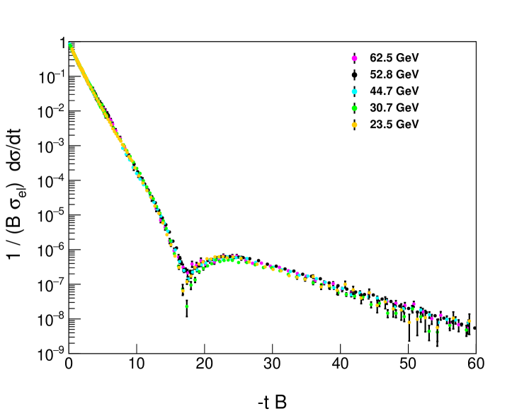
Let us first test these ideas by using the ISR data in the energy range of GeV. The results are shown in Fig. 1 which indicates that the ISR data indeed show a data-collapsing behaviour.
At low values of , the scaling function is indeed, approximately, , that remains a valid approximation over, at least, five orders of magnitude in the decrease of the differential cross section. However, at the ISR energies, the scaling seems to be valid, within the experimental uncertainties, not only at low values of , but extended to the whole four-momentum transfer region, including the dip and bump region as well. Even at large- after the bump region, corresponding to , the data can approximately be scaled to the same, non-exponential scaling function: in the tails of the distribution. Thus, Fig. 1 indeed indicates a non-trivial data-collapsing behaviour to the same, non-trivial scaling function at the ISR energy range of GeV.
This observation motivated us to generalize the derivation presented above in this section, to arbitrary positively definite non-exponential scaling functions . Such a generalisation is performed in the next subsection, in order to give a possible explanation of the data-collapsing behaviour in Fig. 1.
4.4 Generalized scaling functions for non-exponential differential cross-sections
In this section, we search for a novel type of scaling functions of elastic data that may be valid not only in the diffractive cone, but also in the crucial dip and bump region, as well. In Fig. 1, we have noticed that the data-collapsing behaviour may extend well above the small region significantly beyond the diffractive maximum, indicating a clear deviation of the scaling function from the exponential shape.
In addition, a recent detailed study of the low- behaviour of the differential elastic cross section at TeV observed a more than 7-significant deviation from the exponential shape Antchev:2015zza ; Csorgo:2016qyr , which also corresponds to a non-exponentiality in the scaling function even in the low-, or small , range.
In this section, we thus further generalize the derivation of the scaling function, in order to allow for arbitrary positively definite functions with normalisation, and to develop a physical interpretation of the experimental observations.
Let us start the derivation from the relation of the elastic scattering amplitude in the impact parameter space and the complex opacity function based on Eq. (12), using the same notation as in Ref. Nemes:2015iia :
| (41) |
The shadow profile function is equal to the inelastic scattering profile as follows from Eq. (13), . The imaginary part of the opacity function is generally not known or less constrained by the data, but it is experimentally known that is relatively small at high energies: at all the measured LHC energies and below, , hence, %.
Here, we thus follow the choice of Ref. Nemes:2015iia , that has demonstrated that the ansatz
| (42) |
gives a satisfactory description of the experimental data in the GeV2 region, with a small coefficient of proportionality that was denoted in Ref. Nemes:2015iia by parameter. This ansatz assumes that the inelastic collisions at low four-momentum transfers correspond to the cases when the parts of proton suffer elastic scattering but these parts are scattered to different directions, not parallel to one another. This physical interpretation is actually due to and . We will use this approximation below to demonstrate that the scaling function can have more complex shapes, that differ from .
Based on the results of the previous section obtained in the diffractive cone in the and limit, we have the following scaling property of the opacity function:
| (43) | |||||
| (44) | |||||
| (45) | |||||
| (46) |
where is four times the ratio of the elastic to the total cross section, as given in Eq. (27), and describes the distribution of the inelastic collisions as a function of the dimensionless impact parameter normalised to , the characteristic length-scale of the collisions at a given value of the center-of-mass energy .
This ansatz allows for a general shape of the impact parameter -dependent scattering amplitude, that leads to a scaling. Under the assumption that the -dependence may occur only through the two-dimensional scaling variable , as described by the scaling function ,
| (47) |
a general form of the scaling can be obtained. Here we assume that is a real function that depends on the modulus of the dimensionless impact parameter . For normalization, we choose that the Fourier-transform , which also corresponds to the condition
| (48) |
keeping in mind that we have two-dimensional Fourier-transform which at zero is equal to the integral over the two different directions in the impact-parameter space.
Let us investigate first the consequences of the scaling ansatz of Eq. (47) for the shadow profile function . The algebra is really very similar to that of the exponential cone approximation that was implemented above. We obtain the following result:
| (49) | |||||
Evaluating the above relation at and using the normalization condition , we obtain again that the shadow profile at zero impact parameter value has a maximum that is slightly less than unity: . It is interesting to note that the maximum in the profile function is reached at the same threshold (29) as in the case of the exponential cone approximation, corresponding to
| (50) | |||||
| (51) |
Thus a threshold-crossing behaviour seems to happen if the elastic-to-total cross-section ratio exceeds . Remarkably, in the domain of validity of our derivation, this threshold crossing point is independent of the detailed shape of the scaling function for a broad class of models. However, it is also clear from Eq. (49) that the shape of function plays an important role in determining the hollowness effect, so a detailed precision shape analysis is necessary to obtain the significance of this effect.
Starting from the definition, Eq. (2), the scattering amplitude in the -space (47) yields the following form of the differential cross section in the momentum space:
| (52) |
Utilizing Eq. (46), we find that this form of the differential cross section is dependent on the four-momentum transfer squared, , indeed only through the variable , so it is a promising candidate to be a scaling variable.
Now, if we consider the function (52) at the optical point, , we find
| (53) |
If the impact parameter dependent elastic amplitude has an -dependent internal scale and -dependent strength, we thus obtain the following generalized scaling relation for arbitrary elastic scattering amplitudes that satisfy Eq. (47):
| (54) |
This scaling is derived for and , and it indicates that the with a non-exponential scaling function is a very interesting theoretical possibility. Further generalizations of this derivation are possible and interesting but go clearly well beyond the scope of this manuscript, that aims to look for Odderon effects using the experimentally available information on this scaling and its possible violations.
In addition to providing an insight to the meaning of the non-exponential behaviour in the interference (dip and bump) region, the above derivation also clarifies meaning of the normalization of . In particular, the normalization of scaling function on the left hand side of Eq. (54) should be made by the value of the differential cross section at the optical () point as given by Eq. (53). This value for differential cross sections with nearly exponential diffractive cone is indeed approximately equal to . In this case, the normalization condition is maintained, while the integral of becomes unity only for differential cross sections dominated by the exponential cone (i.e. when the integral contribution from the non-exponential tails is several orders of magnitude smaller as compared to the integral of the cone region).
For the total cross section, we find from Eq. (5)
| (55) |
Note that here we have indicated the normalization just for clarity, but one should keep in mind that in our normalization, , and correspondingly, by definition.
As clarified by Eq. (54), the scaling function coincides with the modulus squared of the normalized Fourier-transform of the scaling function , if the elastic amplitude depends on the impact parameter only through its scale invariant combination and if . In this case, the scaling is directly connected to the impact parameter dependence of the elastic amplitude and transforms out the trivial -dependencies coming from , , , and functions. This approximation has enabled us to establish possible physical reasons of this new scaling, and to derive non-exponential shapes for the scaling function and to connect violations of the scaling to the hollowness effect in the shadow profile function of the proton at ultra-high energies. At the time of closing this manuscript, the generalization of the above derivation to a -dependent function is still incomplete, and will be the subject of a separate study. Nevertheless, in our numerical analysis of the scaling, detailed in the subsequent sections, in the comparisons of the scaled differential cross-sections and the deduced Odderon significance we have not imposed any condition. Our analysis is generic and has been done using the published experimental data sets only, without imposing any theoretical assumptions such as a -independent etc.
The above derivation also indicates that it is a promising possibility to evaluate the scaling function directly from the experimental data. It has a clear normalization condition, . Furthermore, in the diffractive cone, for nearly exponential cone distributions, . We have shown in this section, that even if one neglects the possible dependence of , arbitrary positively definite scaling functions can be introduced if the elastic amplitude is a product of -dependent functions, and its impact parameter dependence originates only through an -dependent scaling variable which can be conveniently defined as . Thus, the violations of the scaling may happen if not only the slope parameter , the real-to-imaginary ratio and the integrated elastic and total cross sections and depend on , but also the -dependence of the elastic scattering amplitude starts to change noticeably. Namely, the scaling breaks if the scaling relation gets violated in the above mentioned case.
Let us also note that the leading-order exponential shape of can be derived as a consequence of the analyticity of at corresponding to the optical point, as follows. By leading order we mean the result of a first-order Taylor series expansion at , so that , although beyond this approximation the functional behaviour of the function cannot be determined from analyticity. If is an analytic function at , then its leading-order behaviour is , where is a complex coefficient that is in general dependent on . Hence, in this approximation the differential cross-section behaves as corresponding to the scaling function in the diffractive cone. Similar considerations, related to (non)-analyticity of modulus squared amplitudes and Lévy stable source distributions were introduced to Bose-Einstein correlations in high energy physics in Ref. Csorgo:2003uv .
On the other hand, our recent analysis of the differential elastic cross sections in the LHC energy range Csorgo:2018uyp ; Csorgo:2018ruk suggests that the approximation breaks down since the TOTEM experiment observed a significant non-exponential behaviour already in the diffractive cone. In this case, at low values of , nearly Lévy stable source distributions can be introduced, that lead to an approximate behaviour, where In this case, the leading order behaviour is non-analytic, . We have shown in Refs. Csorgo:2018uyp ; Csorgo:2018ruk , at low , such a stretched exponential form with describes the elastic scattering data from ISR to LHC energies reasonably well in a very broad energy range from GeV to TeV.
The main limitation of the above derivation is that although it leads to a scaling, the real-to-imaginary ratio is independent of in this approximation. So let us consider a generalization, where the real to imaginary ratio is not only but also dependent. We will discuss, model independently, such a scenario in terms of the impact parameter dependent elastic scattering amplitude in B. Such a dependence of can actually be realized in a number of physical models. In greater details, we consider one particular model, that has a type of scaling limit and the -dependent scaling violations are related to the -dependence of the opacity parameter in this model. We discuss the emergence of the scaling within a physical model, the so-called Real Extended Bialas-Bzdak model of Refs. Bialas:2006kw ; Bialas:2006qf ; Bialas:2007eg ; Bzdak:2007qq ; Csorgo:2013bwa ; CsorgO:2013kua ; Nemes:2015iia in C. We evaluate the domain of validity of this ReBB model in in D, in order to determine if this domain is including (or not) a kinematic region, where the scaling indicates the Odderon signal.
5 Results in the TeV energy range
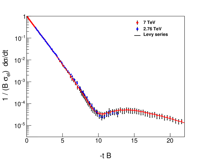
We established that the scaling holds within experimental errors at the ISR center-of-mass energies varying from to GeV, i.e. less than by a factor of three. Let us also investigate the same scaling function at the LHC energies, where the TOTEM measurements span, on a logarithmic scale, a similar energy range, from TeV to TeV, i.e. slightly more than by a factor of four. The TOTEM data at 13, 7 and TeV are collected from Refs. Antchev:2017dia , Antchev:2013gaa , and Ref. Antchev:2018rec , respectively, and plotted in Fig. 2. Note that the possible scaling violating terms are small in the TeV region: they are within the statistical errors, when increasing from 2.76 to 7 TeV, i.e. by about a factor of 2.5. Let us also stress that we do not claim the validity of the scaling up to the top LHC energy of TeV, as scaling violating terms start to be significant at that energy, in particular, close to the diffractive dip region.
Let us look into the scaling behaviour in the energy range of TeV in more detail.
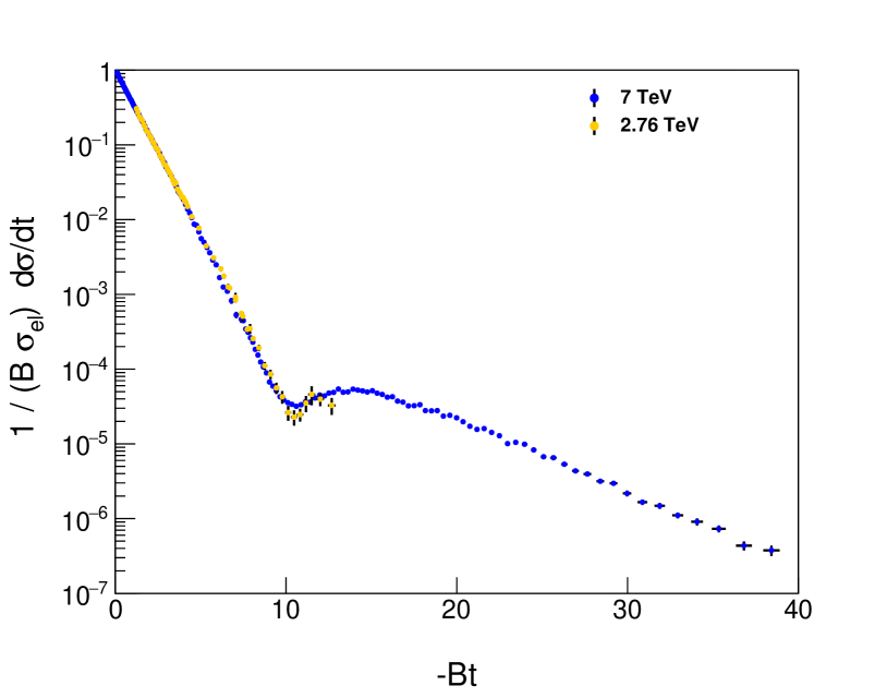
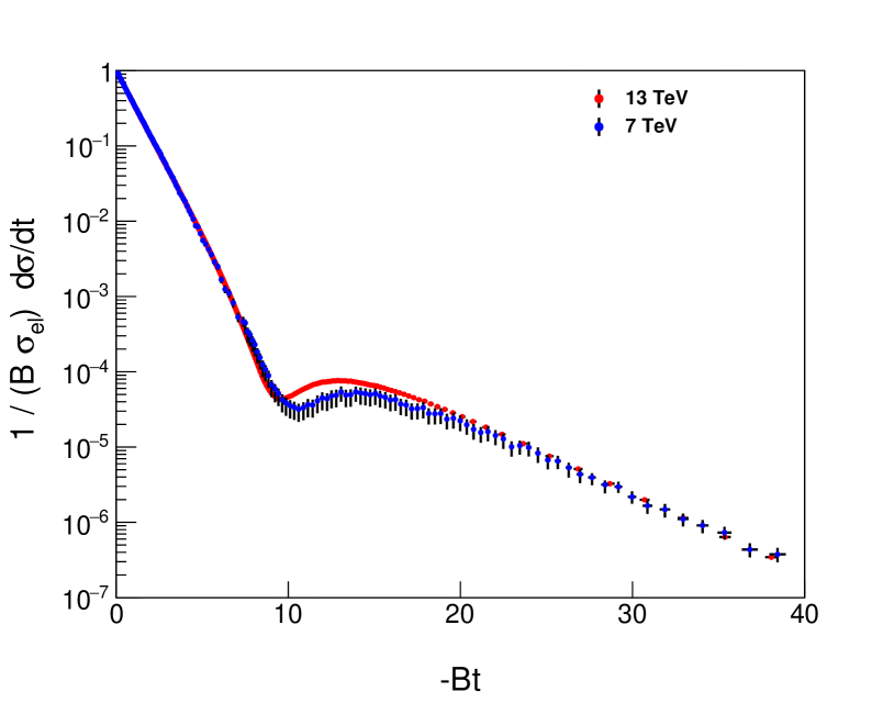
The left panel of Fig. 2 indicates that the scaling valid within statistical errors in the TeV energy range. The confidence level of this comparison corresponds to a CL = 99 % (statistical errors only). The right panel of the same Fig. 2 indicates that this scaling is violated, beyond systematic errors, if the TeV data are also included into this comparison: the violation of the scaling by the 13 TeV data is focused to the region of the diffractive dip. However, in the region, the scaling is approximately valid at each of these LHC energies of , and TeV. Instead of being approximately valid in the whole measurable region, at the LHC this scaling remains valid at all these three LHC energies only through about 3-4 orders of magnitude drop in the differential cross-section at lower values of . The so called “swing” effect becomes clear at TeV: the scaling function starts to decrease faster than exponential before the diffractive mimimum, and also the diffractive minimum moves to lower values in as compared to its position at lower LHC energies. This swing effect, apparent in Fig. 2, can be interpreted in terms of changes in the shadow profile of protons at the LHC energies as the energy range increases from through to TeV. Indeed, such small -dependent scaling violations in the scaling function show the same qualitative picture as what has been observed by the direct reconstruction of the shadow profiles in the TeV energy range in several earlier papers, see for example Refs. Kohara:2017ats ; Dremin:2018urc ; Dremin:2019tgm or our Refs. Nemes:2015iia ; Csorgo:2018uyp ; Csorgo:2018ruk .
Inspecting the left panel of Fig. 2, we find, that the scaling functions agree within statistical errors, if the colliding energy is increased from TeV to 7 TeV. The right panel of the same figure shows that these data change significantly if the colliding energy increases further to TeV. This implies that the possible scaling violating terms are small as they are within the statistical errors, when increasing from 2.76 to 7 TeV, by about a factor of 2.5. We have checked that TOTEM preliminary data at 8 TeV also satisfy this scaling Kaspar:2018ISMD ; Csorgo:2020rlb .
However, this scaling is violated by -dependent terms when increasing from 8 to 13 TeV, and such a scaling violation is significantly larger than the quadratically (maximally) added statistical and -dependent systematic errors, as indicated on the right panel of Fig. 2.
This behaviour may happen due to approaching a new domain, where the shadow profile function of scattering changes from a nearly Gaussian form to a saturated shape, that in turn may develop hollowness at 13 TeV and higher energies. The experimental indications of such a threshold-crossing behaviour were summarized recently in Ref. Csorgo:2019fbf , and are also described above: a new domain may be indicated by a sudden change of in between 2.76 and 7 TeV and, similarly, the crossing of the critical line in multi-TeV range of energies, somewhere between 2.76 and 7 TeV. From the theoretical side, we have previously noted such as drastic change in the size of the proton substructure between the ISR and LHC energy domains from a dressed quark-like to a dressed di-quark type of a substructure Csorgo:2018uyp ; Csorgo:2018ruk which may be, in principle, connected to such a dramatic change in the scaling behaviour of the elastic cross section. However, in this work we focus on the scaling properties of the experimental data, and do not intend to draw model-dependent conclusions. Nevertheless, we use the model-dependent results as well in order to cross-check our model-independent conclusions. Some details of the model-independent calculations are summarized in A and B, while our model-dependent estimates are described in C, D and E.
In Fig. 3 we directly compare the scaling functions of the differential cross sections, using the same ISR and LHC data, as in Figs. 1 and 2, respectively. This range of data now spans nearly a factor of about 500, about a three orders of magnitude increase in the range of available colliding energies, from 23.5 GeV to 13 TeV. As can be seen in the corresponding Fig. 3, the scaling works approximately in the diffractive cone, however, the scaling function cannot be considered as an approximately constant if such a huge change in the colliding energies is considered.
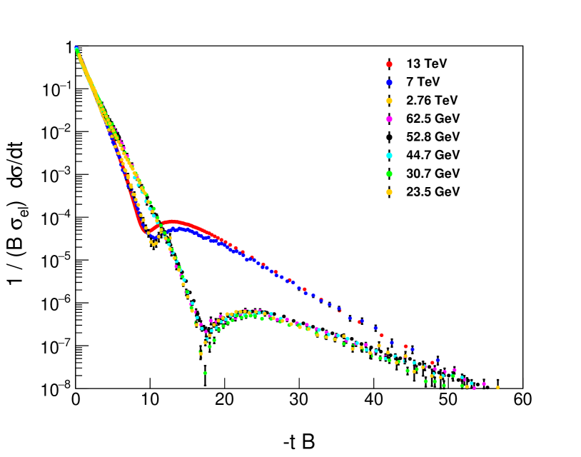
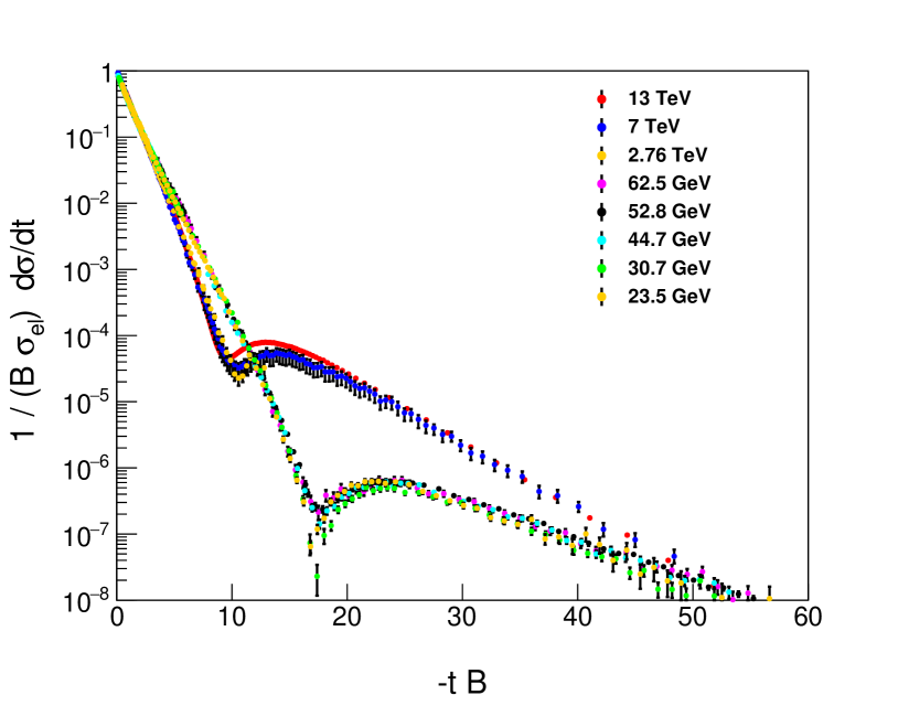
Comparing Figs. 1, 2 and 3, we find that the -dependence of the scaling functions is rather weak if changes within a factor of two, however, there are very significant changes if the range of energies is changing by a factor of a few hundred, from the ISR energy range of GeV to the LHC energy range of 2.76 – 7.0 – 13.0 TeV.
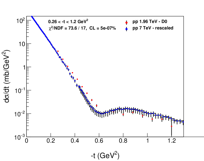
In the left panel of Fig. 4, the function of the TeV TOTEM data set of Ref. Antchev:2018rec is compared with that of the collisions measured by the D0 collaboration at TeV Tevatron energy Abazov:2012qb . The right panel of Fig. 4 compares the scaling functions of elastic collision at TeV LHC energy Antchev:2011zz ; Antchev:2013gaa to that of the elastic collisions at the Tevatron energy, TeV. On both panels, the statistical errors and -dependent systematic errors are added in quadrature. Lines are shown to guide the eye corresponding to fits with the model-independent Lévy series studied in Refs. Csorgo:2018uyp ; Csorgo:2018ruk . These plots suggest that the comparison of the scaling functions or elastic to collisions in the TeV energy range is a promising method for the Odderon search, and a precise quantification of the difference between the scaling functions for to collisions data sets is important. But how big is the difference between the scaling functions of elastic collisions at similar energies?
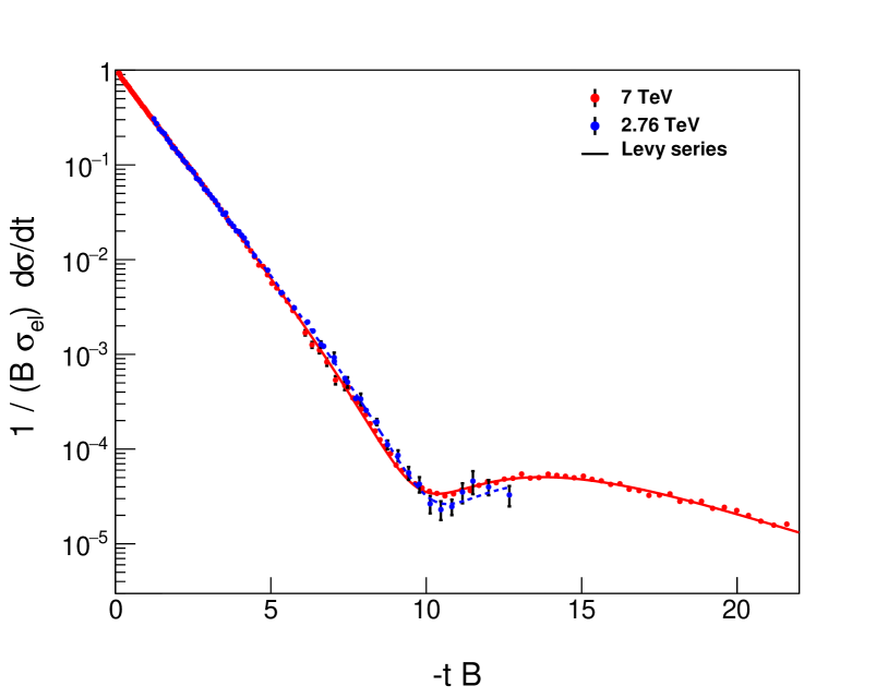
The scaling of the differential cross section of elastic collisions is compared at the nearby and TeV LHC energies in Fig. 5. These plots are similar to the panels of Fig. 4. The scaling functions are remarkably similar, in fact, they are the same within the statistical errors of these measurements. Due to their great similarity, it is important to quantify precisely how statistically significant their difference is.
We stress in particular that the possible scaling violations are small, apparently within the statistical errors, when results are compared at LHC energies and is increased from 2.76 to 7 TeV, by about a factor of 2.5. This makes it very interesting to compare the differential cross-sections of and elastic scattering at the nearest measured energies in the TeV range, where crossing-odd components are associated with Odderon effects. Actually, the largest of elastic scattering data is 1.96 TeV Abazov:2012qb while at the LHC the public data set on the elastic scattering is available at TeV Antchev:2018rec , corresponding to a change in by a factor of . This is a rather small multiplicative factor on the logarithmic scale, relevant to describe changes both in high energy and collisions. Given that the scaling function is nearly constant between 2.76 TeV and 7 TeV within the statistical errors of these data sets, we will search for a significant difference between the scaling function of elastic collisions at and TeV as well as that of the elastic scattering at TeV. If such a difference is observed, then there must be a crossing-odd (Odderon) component in the scattering amplitude of elastic and scatterings.
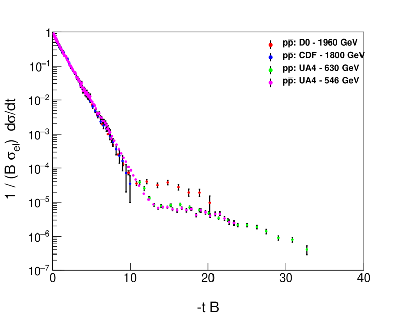
Let us now consider Fig. 6. This plot compares the scaling functions for collisions at various energies from GeV to 1.96 TeV. Within experimental errors, an exponential cone is seen that extends to at each measured energies, while for larger values of the scaling law breaks down in an energy dependent manner. At lower energies, the exponential region extends to larger values of , and the tail regions are apparently changing with varying colliding energies. Due to this reason, in this paper we do not scale the differential cross section of elastic collisions to different values of as this cannot be done model-independently. This property of elastic collisions is in contrast to that of the elastic collisions, where we have demonstrated in Figs. 1,2 that in a limited energy range between and GeV, as well as at the LHC in the energy range between and TeV, the scaling works well. Due to these experimental facts and the apparent violations of the scaling for collisions in the region, in this paper we do not attempt to evaluate the energy dependence of the differential cross sections for collisions. However, based on the observed scaling in collisions, we do find a model-independent possibility to rescale the differential cross sections of elastic collisions in limited energy ranges.
After the above qualitative discussion of scaling for both and elastic collisions, let us work out the details of the possibility of rescaling the measured differential cross sections to other energies in the domain where indicates a scaling behaviour within experimental errors.
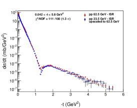
The left panel of Fig. 7 indicates the result of rescaling of the differential cross sections of elastic scattering from the lowest GeV to the highest GeV ISR energy, using Eq. (67). We have evaluated the level of agreement of the rescaled 23.5 GeV data with the measured 62.5 GeV data with the help of Eq. (60). The result indicates that the data measured at GeV and duly rescaled to 62.5 GeV are, within the errors of the measurements, consistent with the differential cross section of elastic collisions as measured at GeV. This demonstrates that our method can also be used to extrapolate the differential cross sections at other energies by rescaling, provided that the scaling is not violated in that energy range and that the nuclear slope and the elastic cross sections are known at a new energy as well as at the energy from where such a rescaling starts.
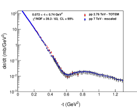
A similar method is applied at the LHC energies in the middle panel of Fig. 7. This plot also indicates a clear agreement between the 2.76 TeV data and the rescaled 7 TeV data, which corresponds to a and a CL of 99.2 % and a deviation on the 0.01 level only. This suggests that indeed the rescaling of the differential cross section of elastic scattering can be utilized not only in the few tens of GeV range but also in the few TeV energy range. Most importantly, this plot indicates that there is a scaling regime in elastic collisions, that includes the energies of 2.76 and 7 TeV at LHC, where the scaling is within errors, not violated. This is in a qualitative contrast to the elastic collisions at TeV energies, where the validity of the scaling is limited only to the diffractive cone region with , while at larger values of , the scaling is violated.
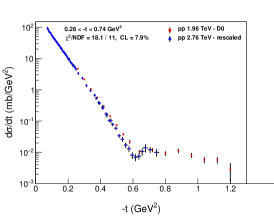
The right panel of Fig. 7 indicates a surprising agreement: after rescaling of the differential cross section of elastic collisions from 2.76 TeV to 1.96 TeV, we find no significant difference between the rescaled 2.76 TeV data with the data at the same energy, TeV. The agreement between the extrapolated and the measured differential cross sections correspond to an agreement at a CL of 7.9 %, i.e. a surprising agreement at the level. It can be seen on the right panel of Fig. 7 that in the swing region, before the dip, the rescaled differential cross section seems to differ qualitatively with the collisions data. However, according to our analysis that also takes into account the horizontal errors of the TOTEM data, we find that this apparent qualitative difference between these two data sets is quantitatively not significiant: it is characterized as an agreement within less than 2.
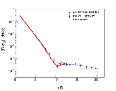
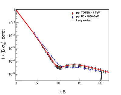
These plots suggest that the scaling functions of elastic and collisions differ at similar energies, while the same scaling functions for elastic collisions are similar at similar energies, thus the comparison of the scaling functions of elastic and collisions is a promising candidate for an Odderon search. Due to this reason, it is important to quantify how significant is this difference, given that the scaling functions scale out the dominant -dependent terms, that arise from the energy-dependent and functions. Such a quantification is the subject of the next section.
Before going into more details, we can already comment on a new Odderon effect qualitatively. When comparing the scaling function of the differential cross section of elastic collisions at 2.76 and 7.0 TeV colliding energies, we see no qualitative difference. By extrapolation, we expect that the scaling function may be approximately energy independent in a bit broader interval, that extends down to 1.96 TeV. Such a lack of energy evolution of the scaling function of the collisions is in a qualitative contrast with the evolution of the scaling functions of collisions at energies of TeV, where a qualitative and significant energy evolution is seen in the kinematic range. Thus, our aim is to quantify the Odderon effect in particular in this kinematic range of in order to evaluate the significance of this qualitative difference between elastic and collisions.
6 Quantification with interpolations
In this section, we investigate the question of how to compare the two different scaling functions with introduced above measured at two distinct energies. We would like to determine if two different measurements correspond to significantly different scaling functions , or not. In what follows, we introduce and describe a model-independent, simple and robust method, that enables us to quantify the difference of datasets or measurements. The proposed method takes into account the fact that the two distinct measurements may have partially overlapping acceptance in and their binning might be different, so the datasets may correspond to two different sets of values.
Let us first consider two different datasets denoted as , with . In the considered case, , consists of a set of data points located on the horizontal axis at different values of , ordered as , are the measured values of at points, and is the corresponding error found at point.
In general, two different measurements have data points at different values of . Let us denote as the domain of , and similarly stands for the domain of . Let us choose the dataset which corresponds to . In other words, is the dataset that starts at a smaller value of the scaling variable as compared to the second dataset . If the first dataset ends before the second one starts, i.e. when , their acceptances would not overlap. In this limiting case, the two datasets cannot be compared with our method. Fortunately, however, the relevant cases e.g. the D0 data on elastic collisions at TeV have an overlapping acceptance in with the elastic collisions of TOTEM at , 7 and 13 TeV. So from now on we consider the case with .
If the last datapoint in satisfies , then is within the acceptance of . In this case, let us introduce as the final point with the largest value of from . If has , then the overlapping acceptance ends at the largest (final) value of index such that . This means that the point of is below the largest value of in , but the next point in is already above the final, largest value of in .
The beginning of the overlapping acceptance can be found in a similar manner. Due to our choice of as being a dataset that starts at a lower value, , let us determine the initial point in that already belongs to the acceptance domain of . This is imposed by the criterion that .
We compare the and datasets in the region of their overlapping acceptance, defined above, either in a one-way or in a two-way projection method. The projection has the number of degrees of freedom NDF equal to the number of points of in the overlapping acceptance. For any of such a point , we used linear interpolation of the nearest points from such that in order to evaluate the data and the errors of at this particular value of . This is done employing a default (linear, exponential) scale in the plane, that is expected to work well in the diffraction cone, where the exponential cone is a straight line. However, for safety and due to the unknown exact structure at the dip and bump region, we have also tested the linear interpolation utilizing the (linear, linear) scales in the plane.
Similarly, the projection has the number of degrees of freedom NDF as the number of points of dataset that fell into the overlapping common acceptance. A linear extrapolation was used for each points in this overlapping acceptance, so that , using both (linear, exponential) and (linear, linear) scales in the -planes. For the two-way projections, for example , the number of degrees of freedom is the sum of the points of and in the overlapping acceptance, defined as NDF = NDF + NDF.
Let us describe the two-way projections in more detail as the one-way projections can be considered as special cases of this method. A common domain in the region of the overlap of the and domains can be introduced as follows. Take the data points in the interval from the set and the data points in the interval from the set. This selection procedure provides a total of points. Let us order this new set of points and denote such a united domain as . This domain corresponds to a common acceptance region which has data points on the horizontal axis denoted as .
In order to compare the datasets and , one needs to build two analog datasets that are both extrapolated to the same common domain starting from and as if the data in both analog datasets were measured at the same values of . So far, either or has some data value on any element of the domain , but only one of them is determined.
Let us take first those points from that belong to , and label them with index. There are such points. For such points, the data and error-bars of the extrapolated data set will be taken from : , . However, for the same points, has no measured value. But we need to compare the data of and at common values of . So data and errors can be interpolated using linear or more sophisticated interpolation methods. If the binning is fine enough, linear interpolation between the neighbouring datapoints can be used.
At this point, let us consider that in the diffractive cone, when an exponential approximation to the differential cross section can be validated, the shape of the scaling function is known to be . This function is linear on a (linear, logarithmic) plot of . In what follows, we will test both a (linear, exponential) interpolation in the plots (that is expected to give the best results in the diffractive cone) and a (linear, linear) interpolation that has the least assumptions and that may work better than the (linear, exponential) interpolation technique around the diffractive minimum. These two different interpolation methods also allow us to estimate the systematic error that comes from the interpolation procedure itself. If the data points are measured densely enough in the plot, both methods are expected to yield similar results. We present our final results using both techniques and note that indeed we find similar results with both methods.
Suppose that for the -th point of data set and for some value of , . Then a linear interpolation between the -th and -th point of yields the following formula:
| (56) |
Similarly, the errors can also be determined by linear interpolation as
| (57) |
This way, one extends to the domain , corresponding to the overlapping acceptance of two measurements. If there is a measured value in , we use that value and its error bar. If there is no measurement in precisely at that given value of that is part of the overlapping acceptance (corresponding to a value from ) then we use the two neighbouring points from and use a (linear) interpolation to estimate the value at this intermediate point. This method works if the binning of both data sets is sufficiently fine so that non-linear structures are well resolved.
This way, for those points from that belonged to , we have defined the data values from by identity and defined the data points from by linear interpolation from the neighbouring bins, so for these points both data sets are defined.
A similar procedure works for the remaining points in that originate from . The number of such points is . Let us index them with . For these points, data and error-bars of the extrapolated data set will be taken from : , while the errors are given as . However, for the same points, has no measured value. As we need to compare the data of and at common values of , for these points, data and errors can be extrapolated using the linear or more sophisticated interpolation methods based on the nearest measured points. If the binning is fine enough, linear interpolation between the neighbouring data-points can be appropriately used. For broader bins, more sophisticated interpolation techniques may also be used that take into account non-linear interpolations based on more than two nearby bins, for example interpolations using Levy series expansion techniques of Ref. Csorgo:2018uyp . However, in the present manuscript such refinements are not necessary as the (linear, linear) and the (linear, exponential) interpolations in () give similar results.
Consider now that for the -th point of data set and for some -th value of , . Then linear interpolation between the -th and -th point of yields the following formula:
| (58) |
Similarly, the errors can also be determined by linear interpolation as
| (59) |
This way, using the linear interpolation techniques between the neighbouring data points, we can now compare the extended and to their common kinematic range: was embedded and extrapolated to data points and errors denoted as and while was embedded and extrapolated to data points and errors denoted as and , respectively. Note that the domain of both of these extended data sets is the same domain. The index “12” indicates that was extended to , while index “21” indicates that was extended to domain .
Now, we are done with the preparations to compare the two data sets, using the following definition:
| (60) |
In this comparison, there are no free parameters, so the number of degrees of freedom is NDF , the number of data points in the unified data sample.
Based on the above Eq. (60) we get the value of and NDF, which can be used to evaluate the -value, or the confidence level (CL), of the hypothesis that the two data sets represent the same scaling function. If CL satisfies the criteria that CL , the two data sets do not differ significantly. In the opposite case, if CL the hypothesis that the two different measurements correspond to the same a priori scaling function, can be rejected.
The advantage of the above definition by Eq. (60) is that it is straightforward to implement it, however, it has a drawback that it does not specify how to deal with the correlated or dependent errors, and horizontal or errors. The measurements at TeV are published with their horizontal errors according to Table 5 of Ref. Antchev:2013gaa . These errors should be combined with the published errors on the nuclear slope parameter to get a horizontal error on indicated as . Such a horizontal error has to be taken into account in the final calculations of the significance of the Odderon observation.
Regarding the correlations among the measured values, and the measured errors, the best method would be to use the full covariance matrix of the measured differential cross section data. However, this covariance matrix is typically unknown or unpublished, with an exception of the TeV elastic measurement by TOTEM Antchev:2018edk . Given that this TOTEM measurement of at 13 TeV indicates already the presence of small scaling violating terms in according to Fig. 2, this 13 TeV dataset cannot be used directly in our Odderon analysis, that is based on the -independence of the scaling function of the differential elastic cross section in a limited range that includes 2.76 and 7 TeV, but does not extend up to 13 TeV. However, we can utilize this TOTEM measurement of at 13 TeV, to test the method of diagonalization of the covariance matrix that we apply in our final analysis of the Odderon significance.
Our analysis of the covariance matrix relies on a method developed by the PHENIX Collaboration and described in detail in Appendix A of Ref. Adare:2008cg . This method is based on the following separation of the various types of experimental uncertainties:
Type A errors are point-to-point uncorrelated systematic uncertainties.
Type B errors are point-to-point varying but correlated systematic uncertainties, for which the point-to-point correlation is 100 %, as the uncorrelated part is separated and added to type A errors in quadrature.
Type C systematic errors are point-independent, overall systematic uncertainties, that scale all the data points up and down by exactly the same, point-to-point independent factor.
Type D errors are point-to-point varying statistical errors. These type D errors are uncorrelated statistical errors, hence they can be added to the also uncorrelated, type A systematic errors in quadrature.
In this paper, where we apply this method to compare two different scaling functions, we also consider a fifth kind of error, type E that corresponds to the theoretical uncertainty, which we identify with the error of the interpolation of one of the (projected) data sets to the values that are compared at some (measured) values of to a certain measured data point at a measured value. This type E error is identified with the value calculated from the linear interpolation, described above, as given for each A, B, C and D type of errors similarly by Eq. (59). Type D errors are added in quadrature to type A errors, and in what follows we index these errors with the index of the data point as well as with subscripts , and , respectively.
Using this notation, Eq. (A16) of Ref. Adare:2008cg yields the following definition, suitable for the projection of dataset to , or :
| (61) | |||||
where is the type A uncertainty of the data point of the united data set scaled by a multiplicative factor such that the fractional uncertainty is unchanged under multiplication by a point-to-point varying factor:
| (62) |
In these sums, there are NDF number of data points in the overlapping acceptance from dataset . A similar sum describes the one-way projection , but there are NDF points in the common acceptance. For the two-way projections, not only the number of degrees of freedom add up, , but also the values are added as .
Let us note at this point, that is a scaling function that is proportional to the differential cross section normalized by the integrated cross section. In this ratio, the overall, type C point-independent normalization errors multiply both the numerator and the denominator, hence these type C errors cancel out in . Given that these type C errors are typically rather large, for example, 14.4 % for the D0 measurement of Ref. Abazov:2012qb , it is an important advantage in the significance computation that we use a normalized scaling function . So in what follows, we set and rewrite the equation for the definition accordingly. This effect increases the significance of a -scaling test.
The price we have to pay for this advantage is that we have to take into account the horizontal errors on in order to not overestimate the significance of our test. In this step, we follow the propagation of the horizontal error to the as utilized by the so-called effective variance method of the CERN data analysis programme ROOT. This yields the following definition that we have utilized in our significance analysis for the case of symmetric errors in :
| (63) |
where is the (symmetric) error of in the -th data point of the data set , and is the numerically evaluated derivative of the extrapolated value of the projected data point obtained with the help of a linear interpolation using Eq. (58). Such definition is valid when the type B errors are known and are symmetric for the data set and the errors on are also symmetric. When the data set corresponds to the D0 measurement of elastic collisions, Ref. Abazov:2012qb , we have to take into account that D0 did not publish the separated statistical and -dependent systematic errors, but decided to publish their values added in quadrature. So we use these errors as type A errors and with this method, we underestimate the significance of the results as we neglect the correlations among the errors of the data points in the D0 dataset. The TOTEM published the -dependent statistical type D errors and the -dependent systematic errors both for the 2.76 TeV and 7 TeV measurements of the differential cross sections Antchev:2011zz ; Antchev:2013gaa ; Antchev:2018rec , with the note that the -dependent systematic errors are almost fully correlated. In these works, TOTEM did not separate the point-to-point varying uncorrelated part of the -dependent systematic errors. We thus estimate the type A errors by the statistical errors of these TOTEM measurements, we then slightly underestimate them, hence overestimate the and the difference between the compared data sets. Given that they are almost fully correlated, we estimate the type B errors by the point-to-point varying almost fully correlated systematic errors published by the TOTEM. We have tested this scheme by evaluating the from a full covariance matrix fit and from the PHENIX method of diagonalizing the covariance matrix at TeV, using the Lévy expansion method of Ref. Csorgo:2018uyp . We find that the fit with the full covariance matrix results in the same minimum within one standard deviation of the fit parameters, hence the same significance as the fit with the PHENIX method of Appendix A of Ref. Adare:2008cg .
We have thus validated the PHENIX method of Ref. Adare:2008cg for the application of the analysis of differential cross section at TeV, together with the effective variance method of the ROOT package. This validation is important as the full covariance matrix of the TeV and TeV measurements by TOTEM is not published, but the PHENIX method appended with the ROOT method of effective variances can be used to effectively diagonalize the covariance matrix and to get similar results within the errors of the analysis. In Section 9, we employ the preliminary definition of Eq. (63) to estimate the significance of the Odderon signal in comparison of the scaling functions for elastic and collisions. Our final definition and the corresponding final results are described in A.
7 Extrapolation of the differential cross-sections
In this section, we discuss how to extrapolate the data points to energies where measurements are missing. We emphasize that this method is not our best method to evaluate the significance of the Odderon signal, but we include this section for the sake of completeness, as other groups follow this method. The obvious reason for this is that a large, 14.4 % overall correlated, type C error of the D0 measurement does not cancel from the differential cross-sections, and their significances, while it simply cancels from the scaling functions, that are normalized to the integral of the differential cross-section. A quantitative estimate of the importance of this effect is shown in A, and we detail the results from the comparison of the scaling functions starting from the next section. We recommend this section to those readers, who are motivated to understand how to extrapolate the differential cross-sections to a new, not measured energy in a domain of where the scaling is known to be valid from already performed measurements.
We have found, for example, that in the ISR energy range of – GeV the scaling function is approximately independent of within errors, and with a possible exception at a small region around the diffractive minimum. We show how to extrapolate data points to unmeasured energies, under the condition that in a given energy range, is independent of the collision energy, . In general, such a feature has to be established or cross-checked experimentally. This case is important, given that we have shown before, for example in Fig. 5, that for collisions stays energy-independent within errors between the LHC energies of TeV TeV. Furthermore, we have already shown that for collisions, in the energy range of 0.546 TeV, as indicated in Fig. 6.
Let us denote two different center-of-mass energies between which within the experimental errors as and . Analogically, we denote various observables as , , .
The energy independence of the scaling function formally can be written as
| (64) |
This simple statement has tremendous experimental implications. The equality means that the scaling function is the same, if at center-of-mass energy it is measured at and at energy it is measured at , so that
| (65) |
The equality is expressed as
| (66) |
Putting these equations together, this implies that the experimental data can be scaled to other energies in an energy range where is found to be independent of as follows:
| (67) |
With the help of this equation, the data points on differential cross sections can be scaled to various different colliding energies, if in a certain energy region the scaling holds within the experimental errors. In other words, the differential cross section can be rescaled from to by rescaling the -variable using the ratio of , and by multiplying the cross section with the ratio .
8 Results
In this section, we present our results and close the energy gap, as much as possible without a direct measurement, between the TOTEM data on elastic collisions at and TeV and D0 data on elastic collisions at TeV. This section is based on the application of Eq. (67) in this energy range. After the rescaling procedure, the resulting data set at the new energy is compared with the measured data quantitatively with the help of Eq. (60).
We have used the rescaling equation, Eq. (67) first to test and to cross-check, if the rescaling of the GeV ISR data to other ISR energies works, or not. The left panel of Fig. 7 indicates that such a rescaling of the differential cross sections from the lowest ISR energy of to the highest ISR energy of GeV actually works well. The level of agreement of the rescaled 23.5 GeV data with the measured 62.5 GeV data has been evaluated with the help of Eq. (60). We found an agreement with a , corresponding to a CL = 21.3 % and a difference is at the level of 1.25 only. This result demonstrates that our rescaling method can also be used to get the differential cross sections at other energies, provided that the nuclear slope and the elastic cross sections are known at the new energy as well as at the energy from where we start the rescaling procedure.
Subsequently, one can also rescale the TOTEM data at or TeV to TeV, given that is (within errors) energy independent in the range of TeV, corresponding to nearly a factor of 2.5 change in , while the change in from to TeV is only a factor of 1.4. The right panel of Fig. 7 indicates that rescaling of the differential elastic cross section from to TeV also gives valuable results. We have evaluated the confidence level of the comparison of the rescaled 2.76 TeV data with the 1.96 TeV data with the help of Eq. (60). As was already mentioned above, we have found a surprising agreement with a , corresponding to a CL = 7.93 %, and a difference at the level of 1.75 only.
Another important result is illustrated in Fig. 8. This comparison indicates a difference between the rescaled 7 TeV elastic differential cross-section Antchev:2011zz ; Antchev:2013gaa to the 1.96 TeV energy and to the corresponding data measured at TeV Abazov:2012qb . To obtain a first estimate, this difference is quantified with the help of Eq. (60) yielding a CL of %, which corresponds to a difference at the 5.84 level. As this method adds the statistical and the point-to-point varying systematic errors in quadrature, it underestimates the actual significance of the difference between the two data sets. Although this estimate already provides a significant, greater than 5 effect for the Odderon observation, corresponding to a significant, 5.84 difference between the dataset and the 1.96 TeV dataset, however, the evaluation of this significance does not yet take into account the rather large overall normalization error of 14.4 % that has been published by the D0 collaboration.
This Fig. 8 indicates that not only the diffractive interference, the dip and the bump may carry an Odderon signal, but also the so called swing region, where the differential cross-section bends below the straight exponential diffractive cone of the result. See also Fig. 16 of A for more details on how the type C errors reduce the significance of the Odderon signal to a 3.64, if the comparison is done directly at the level of the differential cross-sections and if these type C, overall correlated errors are added in quadrature to the point-to-point correlated, type A errors. This is only a lower bound of the significance as type C errors are not point-to-point fluctuating, but shift the whole dataset up or down in a correlated way, see the end of A for more details on this lower bound. The point is that it is advantageous to use the scaling function instead of the differential cross-sections, as the rather large type C errors cancel from while they may lead to an important reduction of the significance of the signal when they are considered on the differential cross-sections.
It can be seen in Fig. 8 that in the swing region, before the dip, the rescaled differential cross section differ significantly from that of collisions. Looking by eye, the swing and the diffractive interference (dip and bump) regions both seem to provide an important contribution. We have dedicated E to evaluate the significanes of various regions, to determine precisely how much do they contribute to the significance of this Odderon signal.
The estimates of statistical significances given in the present Section are based on a test that includes the -dependent statistical errors and the -dependent systematic errors added in quadrature. Thus the values of NDF and significances given in this Section can only be considered as estimates. Indeed, although the -dependent systematic errors on these TeV data are known to be almost fully correlated, the covariance matrix is not publicly available at the time of closing this manuscript from the TOTEM measurement at TeV. It is clear that the is expected to increase if the covariance matrix is taken into account, and this effect would increase the disagreement between the measured and the extrapolated differential cross sections at TeV.
So this indicates that we have to consider the proposed rescaling method as conservatively as possible, that allows us to take into account the statistical and -dependent correlated systematic errors, as well as the -independent correlated systematic errors. Such an analysis is presented in the next section, where we quantify the differences between the scaling functions of elastic and collisions using the fact that is free of -independent normalisation errors, and our final results are summarized in A.
9 A significant Odderon signal from the and scaling functions
In this section, we estimate a preliminary, 6.55 significance for the Odderon signal, while A determines and summarizes our final Odderon signal of an at least 6.26 effect. Both results are obtained by comparing the scaling functions of and collisions.
We have found a significant Odderon signal by comparing the scaling functions of the differential cross section of elastic collisions with TeV to that of collisions with TeV, as indicated in Fig. 10. The comparison is made in both possible ways, by comparing the data to the data, and vice versa. The difference between these two datasets corresponds to at least a , giving rise to a CL of % and to a preliminary, 6.55 significance, obtained with the help of Eq. (63). The overall, -independent normalization error of 14.4 % on the D0 data set cancels from this , and does not propagate to our conclusions.
These results are obtained for the mb value of the elastic cross section at TeV, and for the linear-exponential interpolation in . Using this method of interpolation, the nearest points were connected with a linear-exponential line, that corresponds to a straight line on a linear-logarithmic plot in . We have used the published values of the differential cross sections , that of the nuclear slope parameter and the measured value of the elastic cross section for 7 TeV elastic collisions. For the elastic cross section of collisions at TeV, we have numerically integrated the differential cross section with an exponential approximation at very low- that provided us with mb.
We have systematically checked the effect of variations in our interpolation method by switching from the (linear-exponential) in interpolation to a linear-linear one and by changing the value of the elastic collisions from the numerically integrated differential cross-section value of mb, which is an unusually large value, but equals within the quoted 14.4% systematic error to the mb value, that corresponds to the trend published by the Particle Data Group, see the Fig. 51.6, bottom panel, yellow line of Ref. Tanabashi:2018oca . The input values of the nuclear slope parameter and the elastic cross-section are summarized in Table 1, the corresponding results are shown in Tables 2, 3, 4 and 5.
| Energy | Reference | ||
| (GeV) | (mb) | (GeV-2) | |
| 1960 | 17.6 1.1 | Fig. 51.6 of Ref. Tanabashi:2018oca | |
| () | 20.2 1.4 | from low fit to data Abazov:2012qb | |
| 16.86 0.2 | Abazov:2012qb | ||
| 2760 | 21.8 1.4 | Nemes:2017gut | |
| () | 17.1 0.3 | Antchev:2018rec | |
| 7000 | 25.43 1.02 | Antchev:2013iaa | |
| () | 19.89 0.272 | Antchev:2013gaa |
As part of our systematic studies, we have also changed the direction of the projection. The results are summarized in Table 2. They indicate that the improved version of Fig. 8, shown as the top left panel of Fig. 10 and evaluated with the help of our improved definition of Eq. (63) corresponds to a conservative case of Odderon observation based on the TeV TOTEM and the TeV D0 data sets. This panel indicates that the Odderon signal is observed in this comparison with a preliminary, at least a 6.55 significance, indicating the power of our method of Odderon observation. In addition to this, our final result includes a symmetry requirement and a robustness test described in A. These effects decreased the significance of our Odderon observation, from a preliminary, 6.55 effect to a final and statistically significant, 6.26 effect.
We have checked the robustness of this result for several possible variations of the definition. The consideration that was most successful in decreasing this significance was related to the fact that unlike the original PHENIX method of Ref. Adare:2008cg , that was worked out for a theory to data comparison, in this manuscript we compare data to data. So we have adapted the PHENIX method of Ref. Adare:2008cg , from a situation where there was a theoretical function without errors compared to data with errors to a situation where we compare two datasets and both of these datasets have the same type of errors. This slightly decreased the significance of the Odderon signal, from the value of a preliminary, at least 6.55 to the final value of 6.26 , as detailed in A of this manuscript. Given that both significances of the preliminary 6.55 , detailed in this section, and 6.26 , detailed in A are clearly and safely above the 5 discovery threshold, this robustness test did not change our conclusions.
The detailed figures, that show the functions for each of these cases are summarized in the left and right panels of Fig. 9 for the comparison of the 7 TeV TOTEM data set with the 1.96 TeV D0 data set. Each plot indicates a clear, nearly quadratic minimum. The values of at the minima are summarized in Table 2, together with other characteristics of significance, like the confidence level and the significance in terms of standard variations. Similarly, the functions for the comparison of the 2.76 TeV TOTEM data set with the 1.96 TeV D0 data set are summarized in Fig. 11. The values of at the minima are given in Table 3, together with other relevant characteristics.
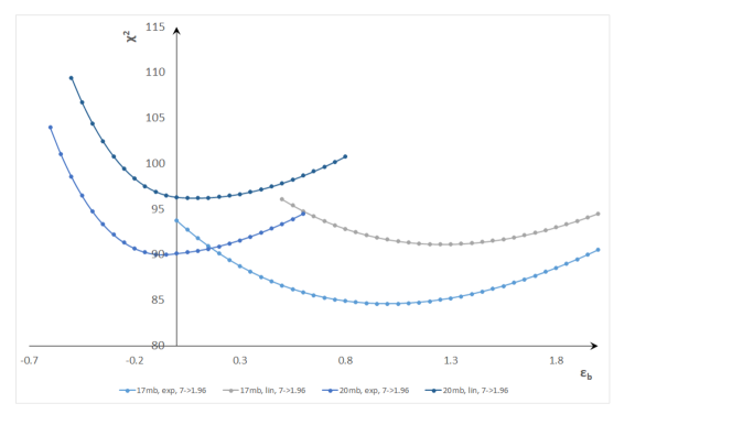
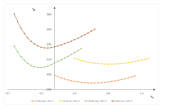
![[Uncaptioned image]](/html/1912.11968/assets/x17.jpg)
As summarized in Fig. 10, a significant Odderon signal is found in the comparison of the scaling functions of the differential elastic (at TeV) vs ( TeV) cross sections. The horizontal error bars are indicated by a properly scaled horizontal line or “” at the data point. The statistical (type A, point-to-point fluctuating) errors are indicated by the size of the vertical error bars (), while shaded boxes indicate the size of the (asymmetric) type B (point-to-point varying, correlated) systematic errors. The overall normalization errors (-independent, type C errors) cancel from the scaling functions since they multiply both the numerator and the denominator of in the same way. The correlation coefficient of the -dependent systematic errors, , is optimized to minimize the based on Eq. (63), and the values indicated in Fig. 10 correspond to the minimum of the . The location of these minima and the best values of depend on the domain in or -range from where the contributions to the are added up. The stability of our final results with respect to the variation of the -range, together with the correlations between the best value of the and the -range are detailed in E. These values, as well as the numbers of degrees of freedom (NDFs) and the corresponding confidence levels (CLs) are indicated on both panels of Fig. 10, for both projections. The functions are summarized in Fig. 9. The 7 TeV 1.96 TeV projection has a preliminary statistical significance of 6.55 of an Odderon signal, corresponding to a and CL = %. A presents the robustness test of this result, and summarizes the result of our tests of various possible modifications of our definition. It turns out that the symmetry requirement discussed in A slightly reduces this significance from a 6.55 level to a 6.26 level, safely above the 5.0 discovery threshold, corresponding to a and CL = %. Thus the probability of Odderon observation in this analysis is at least .
Fig. 10 illustrates some of the results of our systematic studies in four different panels described as follows. The top-left panel of this figure uses a linear-exponential interpolation in the plane and uses the value of 17.6 1.1 mb for the elastic cross section at TeV. This case gives the lowest (6.55) significance for the Odderon observation from among the possible cases that we have considered in Fig. 10. The top-right panel is similar but for a linear-linear interpolation in the . The bottom-left panel is similar to the top-left panel, but now using 20.2 1.4 mb for the elastic cross section at TeV and also using a linear-exponential interpolation in . The bottom-right panel is similar to the bottom-left panel, but using a linear-linear interpolation method.
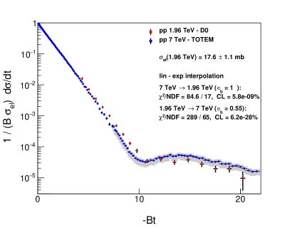


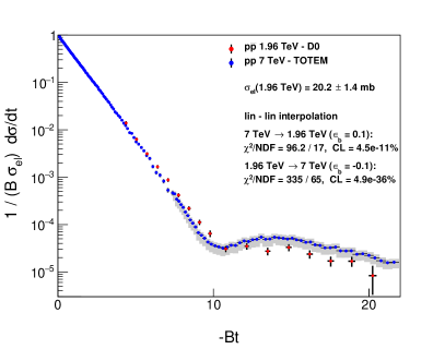
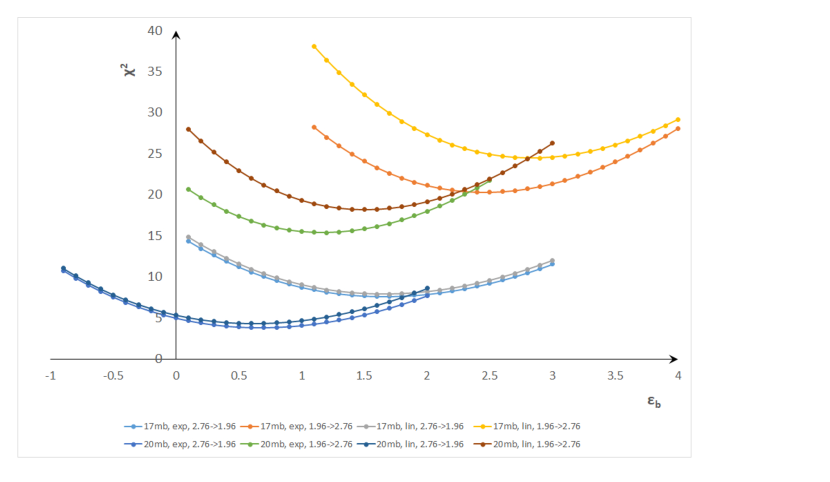
The results of the scaling studies for a comparison of elastic collisions at TeV, measured by the TOTEM experiment at the LHC Antchev:2018rec to that of collisions at TeV, measured by D0 at the Tevatron Abazov:2012qb are summarized in Figs. 11 and 12. The top-left panel of Fig. 12 uses mb and a linear-exponential interpolation method in . The top-right panel is the same as the top-left panel, but for a linear-linear interpolation in . The bottom-left panel is nearly the same as the top-right panel, but for mb. The bottom-right panel is the same as the bottom-left panel, but for a linear-linear interpolation in . Neither of these comparisions shows a significant difference between the scaling function of elastic collisions at TeV as compared to that of collisions at TeV. It seems that the main reason for such a lack of significance is the acceptance limitation of the TOTEM dataset at TeV, which extends up to , in contrast to the acceptance of the 7 TeV TOTEM measurement that extends up to . We have cross-checked this by limiting the 7 TeV data set also to the same acceptance region of as that of the 2.76 TeV data set. This artificial acceptance limitation has resulted in a profound loss of significance, down a to , that corresponds to a CL = 0.71% and to a deviation at the 2.69 level only. This result indicates that if we limit the acceptance of the 7 TeV TOTEM measurement to the acceptance of the 2.76 TeV TOTEM measurement, the significance of the Odderon observation decreases well below the 5 discovery treshold. This result can be understood if we consider, that the diffractive maximum (“bump") is located, if the scaling is valid, at , which is very close but slightly above the value of the upper limit of the acceptance in of the TOTEM data published in Ref. Antchev:2018rec . Fig. 8 of Ref. Antchev:2018rec indicates that indeed the precise location of the diffractive maximum can not be determined from these TOTEM data, it may be just close to the upper limit of the TOTEM acceptance at TeV.
We have thus dedicated E to the scrutiny of the -range dependence of the Odderon signal. In particular, we have investigated how important is the contribution from the large values of . We developed and tested our most conservative definition in A. We have investigated the domain of validity of the scaling with the help of a model and detailed in D, that at TeV, the scaling is expected to hold up to , well above the TOTEM acceptance of . In E, we find that it is sufficient to include a small shift to the investigated range: already for only 10 datapoints from the D0 acceptance the significance of the Odderon signal is greater than in the domain at TeV. In E we also show that the minimum size of subsequent D0 datapoints for a greater than 5 Odderon signal is actually 8 out of 17, corresponding to the range.
We have performed several cross-checks: this topic is detailed in the next section.
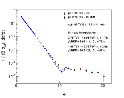

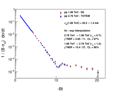
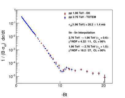
![[Uncaptioned image]](/html/1912.11968/assets/x27.jpg)
![[Uncaptioned image]](/html/1912.11968/assets/x28.jpg)
![[Uncaptioned image]](/html/1912.11968/assets/x29.jpg)
10 A summary of cross-checks
In this section, we summarize some of the most important cross-checks that we performed using our methods and results.
We have cross-checked what happens if one rescales the differential cross section of elastic scattering form the lowest ISR energy of GeV to the top ISR energy of GeV. As can be expected based on the approximate equality of all the scaling functions at the ISR energies, as indicated on the left panel of Fig. 7, the rescaled 23.5 GeV data coincide with the measured 62.5 GeV data. The resulting corresponds to a CL = 21.3 %, or a lack of significant difference – a 1.3 effect. Within errors, our quantitative analysis thus indicates that the two data sets at the ISR energies of 23.5 and 62.5 GeV correspond to the same scaling function, but with possible small deviations in a small -region around the dip position. This indicates that the method that we applied to extrapolate the 2.76 and 7 TeV data sets to lower energies satisfied the cross-checks at the ISR energies, i.e. our method works well. As one of the critical cross-checks of these calculations, two different co-authors coded the same formulae with two different codes using two different programming languages, and these codes were cross-checked against one another until both provided the same values of significances.
We have validated the PHENIX method of Ref. Adare:2008cg implemented in the form of the definition of Eq. (63) for the diagonalization of the covariance matrix on fits to the TeV TOTEM data of Ref. Antchev:2018edk . This PHENIX method resulted, within one standard deviation, the same minimum, hence the same significances, as the use of the full covariance matrix at TeV elastic collisions. At the lower LHC energies of and TeV, due to the lack of publicly available information on the covariance matrix, only the PHENIX method of Ref. Adare:2008cg was available for our final significance analysis.
We have also explored the main reason of the observation of a significant Odderon signal in the comparision of the scaling functions of elastic collisions at TeV with that of the elastic collisions at TeV. The question was rather intriguing as we have found no significant difference between the scaling functions of elastic collisions at = 2.76 TeV and 7 TeV. At the same time, we also see that the comparison of the 2.76 TeV dataset to the 1.96 TeV dataset does not indicate a significant Odderon effect. We have found that the Odderon signal vanishes from the comparison of the 7 TeV and the 1.96 TeV datasets too, if we limit the acceptance of the 7 TeV dataset to the acceptance in as that of the 2.76 TeV dataset: the significance of the Odderon observation decreased from an at least 6.26 discovery effect, detailed in A, to a 2.69 level agreement. We may note that a similar observation was made already in Ref. Ster:2015esa that pointed out a strong dependence of the Odderon contribution.
Table 4 summarises the search for an Odderon signal in the two-way comparison, for the significance of an Odderon signal in the comparison of the scaling functions of collisions at TeV and collisions at TeV. Applying this method the Odderon signal is observed with at least a 13 significance, when both projections are combined from Table 2, by adding the and the NDF values of both directions of the comparisons.
11 Discussion
We have explored the scaling properties of the elastic differential cross sections at various energies, from the ISR up to the highest LHC energy. We have recalled that the earlier proposals for the and scaling functions were useful to explore if elastic scattering of protons in the LHC energy range is already close to the black-disc limit or not. After investigating several possible new dimensionless scaling variables and scaling function candidates, we have realized that in order to look for scaling violations in the low kinematic range, corresponding to the diffractive cone it is advisable to scale all the diffractive cones to the same dimensionless scaling function, . This function can be obtained as the differential cross section normalized to its value at the optical point, which also for nearly exponential distributions equals to the elastic cross section multiplied by the slope parameter . Both are readily measurable in elastic and collisions, while other scaling variables that we have investigated may depend on values – the location of the diffractive minimum. The latter however is not readily accessible neither in elastic collisions (where there is no significant dip) nor in the acceptance limited elastic differential cross section (where the diffractive minimum or maximum may be located outside the acceptance of the experiment for that particular data set).
The scaling function of elastic proton-(anti)proton scattering transforms out the energy dependence of the elastic slope and the elastic cross section , and due to the relation they also scale out a combination of the total cross sections and the real-to-imaginary ratio. As was discussed above, for analytic scattering amplitudes and for differential cross-sections starting with a diffractive cone at low values of the scaling function will have a universal, shape. The price for the removal of these trivial -dependencies from the scaling function is paid by an -depended domain of validity, which is found to be typically above the position of the diffractive interference region. Without direct experimental observations, or without theoretical, model-dependent calculations, it is not possible to determine model-independently this function, the -dependent upper limit of the domain of validity of this scaling.
Figs. 8 and 10 clearly indicate a crossing-odd component of the elastic scattering amplitude. At the 2 TeV energy scale, where the Reggeon contributions to the scattering amplitude are suppressed by their power-law decays, this is apparently a clear Odderon effect, a characteristic difference in the shape of the scaling function of elastic scattering between and collisions at the logarithmically similar energies of 7 and 1.96 TeV, respectively.
The effects due to the energy-induced difference between TOTEM and D0 data sets can be estimated by the lack of change of the scaling function for scattering between 2.76 TeV and 7 TeV, within the statistical errors of these TOTEM data sets. However, the scaling function of elastic scattering at TeV is significantly different from the corresponding result of elastic scattering at TeV. These qualitative and quantitative differences, first, show up well below the diffractive minimum of the elastic scattering, namely, the function for collisions indicates a strong “swing” or faster than exponential decrease effect, before developing a characteristic interference pattern consisting of a diffractive minimum and subsequent maximum. In contrast, the D0 data on elastic scattering features a structureless exponential decrease that in turn changes to a plateaux or a shoulder-like structure at higher values of the scaling variable . No clear indication of a diffractive maximum is seen in the elastic scattering data Abazov:2012qb , while the TOTEM data sets at each LHC energies of 2.76, 7 and 13 TeV clearly indicate a diffractive minimum followed by an increasing part of the differential cross section before the edge of the TOTEM acceptance is reached, respectively Antchev:2018rec ; Antchev:2011zz ; Antchev:2018edk .
These qualitative and quantitative differences between the scaling functions of elastic and scatterings provide a clear-cut and statistically significant evidence for a crossing-odd component in the scattering amplitude in the TeV energy range. This corresponds to the observation of the Odderon exchange in the -channel of the elastic scattering. The Odderon in this context is a crossing-odd component of the amplitude of elastic and scattering, that remains significant even in the large limit. In Regge phenomenology, the Odderon is a trajectory that at contains a vector glueball as well as other glueball states with higher angular momentum. Hence, one of the implications of our result is that not only one but several glueball states should exist in Nature Szanyi:2019kkn .
Due to the presence of the faster-than exponentially decreasing (swing) region in elastic scatterings, high-statistic elastic scattering data at TeV may be taken as an additional measurement clearly closing the energy gap. However, the aperture limitation of the LHC accelerator is already resulting in a loss of significance of the comparison of the scaling function at 2.76 TeV with that of the D0 data at 1.96 TeV. Due to this reason, we propose an additional measurement of the dip and bump region of elastic collisions in the domain where the scaling was shown to work, in between 2.76 TeV and 7 TeV, if that can be harmonized with the LHC running schedule and scenarios.
The current TOTEM acceptance (the upper end of the last bin of the published TOTEM data) ends at at TeV. This value almost coincides with the bump position of the scaling function. It seems that including at least one D0 point to the comparision of the scaling functions of and data above the bump position is sufficient for reaching an at least 5 significance for the Odderon observation, as detailed in E.
New elastic scattering data around 4 – 5 TeV could be particularly useful to determine more precisely any possible residual dependence of these Odderon effects as a function of .
The current significance of the Odderon observation may be further increased from the 6.26 effect, but only by a tedious experimental re-analysis of some of the already published data, for example, by separating the point-to-point uncorrelated statistical and systematic errors (type A errors) from the point-to-point correlated systematic errors in elastic collisions by D0, or, by the publication of the covariance matrix of the elastic cross section measurement of collisions at 2.76 and 7 TeV colliding energies by TOTEM. So taking more TOTEM data in special runs at new energies between and TeV seems to be a more enlightening and inspiring scenario, if it can be harmonized with LHC schedule and other ongoing experimental efforts.
11.1 Discussion of some of our model-dependent results
As noted above, the upper limit of the domain of validity of the scaling, the as a function of cannot be determined model independently, it has to be taken either from extrapolations between different measured points, or from theoretical, model-dependent and validated calculations. Such calculations are presented in A, C and D. One of the most interesting characteristic features of elastic scattering at TeV energies is the presence of a single diffractive minimum and maximum in the experimental data on the differential cross-section of elastic scattering at TeV energies. In terms of the theory of multiple diffraction a single diffractive minimum is obtained if the scattering structures have a two-component internal structure Czyz:1969jg . The model that we have utilized for the evaluation of is based on Refs. Bialas:2006kw ; Bialas:2006qf ; Bialas:2007eg , where the proton is assumed to have a quark-diquark structure, and in one variant of this picture, the diquark is further resolved as a correlated structure, corresponding to the case. As detailed in Ref. Nemes:2015iia , this scenario indeed gives too many diffractive minima in the experimental acceptance, so it can be excluded. Thus our model-dependent results actually also reveal the effective sizes of constituent (dressed) quarks and diquarks inside the protons.
Concerning the quark and diquark sizes, let us note that our values are in qualitative agreement with those obtained first by Bialas and Bzdak in Refs. Bialas:2006kw ; Bialas:2006qf ; Bialas:2007eg at the ISR energies. Already in those papers, the binding energy of the diquark was found to be negligibly small, corresponding to the mass ratio of quarks to diquarks as 1:2. In the model, this mass ratio is reflected in a fixed value for the parameter, that determines the location of their center of mass to the center of the proton. The correlated motion of the quark and the diquark gives an important contribution to the description of the differential cross-section of elastic scattering, as the model of three uncorrelated quarks inside the proton is in a disagreement with the experimental data.
However, the size and existence of the diquarks is a well-known controversy in the literature, related to the interpretation of diquarks. Many scientists theorize that diquarks should not be considered as particles. Even though they may contain two correlated quarks, they are not colour neutral, and therefore cannot exist as isolated bound states. So instead they tend to float freely inside protons as composite entities; while free-floating they have a size of the order of 1 fm. This also happens to be the same size as the proton itself. Other theorists analyzing elastic scattering in the energy range of GeV suggest Dosch:2002ai , that the size of the diquark is much smaller as compared to the size of the protons.
From our Levy studies, published recently in Csorgo:2019egs , it follows, that inside the protons the substructure increases in size, when going from the ISR energies of GeV to the LHC energy of 7.0 TeV, see Fig. 3 and Tables 1, 2 of that paper. So part of the difference of the diquark size in our current manuscript and the sizes obtained in Ref. Dosch:2002ai might be the difference of the investigated energy range, GeV versus our results on the TeV energy scale. Another part of these quantitative differences might be due to the more precise, quantitative, statistically significant level of data description as presented in our paper. The comparison of the diquark sizes is a quantitative question, and it is difficult to make a quantitative comparison with models that were used to describe certain qualitative features of the experimental data, without aiming at a data description on statistically acceptable, significant level.
12 Summary and conclusions
We have introduced a new, straightforwardly measurable scaling function of elastic proton-(anti)proton scattering. This scaling function transforms out the trival energy-dependent factors, in particular, the effects due to the -dependencies stemming from the elastic slope , from the real-to-imaginary ratio , as well as from the total and elastic cross sections, and , respectively. In our numerical re-analysis of already published TOTEM data, the scaling is observed from a comparison of the elastic scattering data at and TeV, without theoretical assumptions. TOTEM preliminary data at TeV are also in the scaling limit, however, published TOTEM data at TeV indicate significant violations of this new scaling. The theoretical background of this scaling law is simple and straightforward in the diffraction cone, where , as detailed in Subsection 4.3. However, the range of the validity of this scaling extends well beyond the diffraction cone already at ISR energies, as shown in Fig. 1. A straightforward theoretical derivation for non-exponential scaling functions was presented in Subsection 4.4.
When comparing the scaling function of the differential cross section of elastic collisions at and TeV colliding energies, we find no qualitative differences. At ISR energies, in a limited energy region of GeV, the scaling curves are approximately -independent, with a possible small scaling violation in the region of the diffractive minimum.
Such a lack of energy evolution of the scaling function of the collisions, even outside the diffractive cone, is in a qualitative contrast with the evolution of the scaling functions of collisions at energies of TeV, where a qualitative and significant energy evolution is seen in the kinematic range for all the investigated energies. This way, we have found a qualitative difference between elastic and collisions in terms of their scaling functions: these functions are not -independent outside the diffractive cone for collisions, while they are approximately -independent in elastic collisions even outside the diffractive cone.
Such a lack of energy evolution of the scaling function of the collisions, the scaling as a property of the data in the few TeV energy range provides a strong constraint on model-building. Several simple models, like the simple eikonal amplitude of one-Pomeron-exchange lead to the violation of such a scaling. It follows that in the few TeV energy range, where the scaling is found to be valid, one-Pomeron exchange cannot be the only contribution to the scattering amplitude.
The main part of our manuscript deals with the quantification of this qualitative Odderon signal, to determine if it is statistically significant, or not.
Figs. 8 and 10 clearly illustrate a qualitative and a quantitative difference between the scaling properties of the elastic and collisions, corresponding to a crossing-odd component of the elastic scattering amplitude at the TeV energy scale. As in this kinematic region the Reggeon contributions to the scattering amplitude are suppressed by their power-law decays, a significant characteristic difference between the scaling functions of elastic and collisions at the logarithmically similar energies of 7, 2.76 and 1.96 TeV is a clear-cut Odderon effect, because the trivial energy dependences of and as well as that of are scaled out from by definition.
A comparison in Fig. 10 indicates a significant difference between the rescaled 7 TeV data set down to 1.96 TeV with the corresponding data measured at TeV. Thus the re-analyzed D0 and TOTEM data, taken together with the verified energy independence of the scaling function in the TeV energy range amount to the closing of the energy gap between 2.76 and 1.96 TeV in model-independent way, as much as reasonably possible without a direct measurement, provided that the scaling is valid for scattering in the kinematic range, where D0 measured the differential cross-section of elastic scattering at TeV.
We have dedicated B to relate the crossing-odd and crossing-even contributions to the elastic and scattering to a model independent and unitary framework, formulated in the impact parameter space. We have specialized the results of B using the model of Ref. Csorgo:2020wmw in C and demonstrated how the scaling and , the collision energy dependent violations of this scaling can be evaluated with the help of this model Csorgo:2020wmw . Note that these calculations are based on R. J. Glauber’s multiple diffraction theory of elastic scattering, assuming that elastic scattering reveals a quark-diquark structure inside the scattered protons. In D, we have determined, model dependently, the domain of validity of the scaling in at TeV. According to Fig. 27, the upper limit for the domain of validity of the scaling at TeV may include the whole D0 acceptance, with . This plot is directly obtained by fitting the scaling limit of the ReBB model to D0 data. In this fit, three out of the four model parameters are constrained by the scaling, so only one physical parameter had to be fitted to achieve a beautiful agreement in a statistically acceptable manner. Another estimate for the upper limit for the domain of validity of the scaling was obtained by comparing the predicted 1 standard deviation error bands of the scaling limit of the ReBB model with the same error band, obtained from the full model calculations that included scaling violations too. This result gave a more conservative upper limit, at TeV. Due to these theoretical uncertainties of the upper limit in of the domain of validity of the scaling at TeV, the highest colliding energy, where elastic scattering data are available, we have investigated the stability of the Odderon signal within the theoretically determined domain of validity of the scaling in E.
Our final significance analysis is presented in A, resulting in an at least 6.26, discovery level Odderon effect, if the scaling is valid in the full kinematic range of the D0 measurement, , corresponding to a and CL = %. The probability of this Odderon signal is at least . According to our model dependent calculations, as presented in Fig. 27, the assumption that the domain of validity of the scaling at TeV includes the whole D0 acceptance with , is consistent with the D0 data at the 2.69 level.
We have also performed an -range stability analysis, also model independently, in E. We established, that the significance of the Odderon is greater than , if the scaling is valid in the kinematic domain at TeV. However, we could not determine model independently, what is the domain of validity of the scaling at this energy, as there are no measured data at TeV. So we have included a model dependent estimate of this -range. Using the model of Refs. Bialas:2006kw ; Nemes:2015iia ; Csorgo:2020wmw , that was shown to describe all the experimental data in elastic and scattering in the TeV energy interval and in the domain, we found that the validity in of the scaling at TeV may extend up to , as detailed in D. This interval or domain of validity of the scaling includes the smaller domain, where the signal is larger than 5 . Thus the model independent and at least 5 discovery level Odderon signal is remarkably stable for the variations of the domain of validity of the scaling at TeV: 9 out of the 17 D0 datapoints can be discarded, 5 at large and 4 points at low , and the signal still remains significant enough for a discovery. When we have fitted the scaling limit of the same model to experimental data, as presented in Fig. 27, we found that is also consistent with the description of the D0 data at the 2.69 level. In general, the scaling is not valid for , but in the Real Extended Bialas-Bzdak model, the scaling of elastic collisions induces a one parameter fit to elastic collisions, as three out of four physical model parameters are the same in this model for and collisions.
Our -range stability analysis, detailed in E, indicates that part of the statistically significant contribution to this Odderon signal is coming from the kinematic range of : excluding this region decreases the significance of the crossing-odd signal below the discovery level. It is thus important to measure elastic scattering cross-sections at LHC at large , well beyond the diffractive cone. Elastic scattering data in a vicinity of 2 TeV as well as in between 2.76 and 7 TeV would be most useful for further detailing the Odderon properties. Similarly, part of the signal is coming from large region, as excluding the kinematic range also results in a loss of significance.
In order to determine where the important contributions to this signal are originating from, we have divided the kinematic range of acceptance to four regions, the diffractive cone, the swing, the diffractive interference and the tail regions, corresponding to , , and , respectively, with 2 D0 points associated with the diffractive cone, and 5-5 D0 points in each of the remaining three regions. We have shown that the type B, point dependent but overall correlated errors and their correlation coefficient plays an important role in this analysis and that the best value of the correlation coefficient is -range dependent. This means that locally shifting the datapoints up or down in a specific interval the agreement between the and measurements can be improved in that particular interval. We have performed the interval dependent optimizations and found that the locally optimized contributions from the swing and from the tail are not as important as the contributions from the diffractive interference region, that includes the diffractive minimum and the maximum. The second most important contribution comes from the swing region, where the scaling function for elastic collisions bends below the exponential. The combination of the swing and the diffractive interference region already provided a more than 5 effect, as detailed in E. If we consider that the interpolations needed to compare the scaling functions in a model-independent manner at different energies behave as theoretical curves (i.e. have only one kind of error) then we obtain the significance of at least 6.55 as discussed in the body of this manuscript. This significance further decreases to 6.26 if we consider that these interpolation lines do not have theoretical type of errors but both type A and type B, point-to-point fluctuating and point-to-point correlated systematic experimental errors as well. The only way to further decrease the significance of the Odderon signal is to limit the kinematic range of the comparison to narrower and narrower ranges in .
Our final significance for an Odderon signal of is presented from the model-independent analysis in A, which relies on the validity of the scaling in the kinematic range at TeV. The self-consistency of this assumption is shown in Fig. 27.
Let us emphasize, for the sake of completeness, that we find an interesting hierarchy of significances.
Based on model dependent considerations, the -range of the data of the D0 experiment might be narrowed and correspondingly, the significances may decrease, as more and more datapoints are removed. Model dependently, we estimate, that the scaling may be valid at the D0 energy of TeV up to . In the , theoretically limited -range the Odderon signal remains greater than , according to E. We have investigated how far this domain can be narrowed down under the condition that the Odderon signal remains greater than a 5 effect? We found that in the very much narrowed from below and from above domain, corresponding to the interval that includes only 8 out of the 17 D0 points, the Odderon signal that we analyzed has a significance that is greater than a 5 , discovery level effect. This range is well below the theoretically estimated limit.
In B, we discuss the model-independent properties of the Pomeron and Odderon exchange at the TeV energy scale, under the condition that this energy is large enough that the Pomeron and Odderon exchange can be identified with the crossing-even and the crossing-odd contributions to the elastic scattering, respectively. We demonstrated here that -matrix unitarity strongly constrains the possible form of the impact parameter dependence of the Pomeron and Odderon amplitudes.
In C, we demonstrated how the scaling emerges within a specific model, defined in Ref. Nemes:2015iia . This model is one of the possible models in the class discussed in B. We have demonstrated that four conditions must be satisfied simultaneously. One of the conditions for the validity of the scaling is found to be the -independence of the experimentally measured parameter. The decrease of at the currently maximal LHC energy of TeV as measured by the TOTEM Collaboration in Ref. Antchev:2017yns thus provides a natural explanation for the violation of the scaling at these energies.
In D we estimate the domain of validity of the scaling also in a model-dependent manner, using the same model of Ref. Nemes:2015iia . Surprisingly, we found that after carefully taking into account the possible quadratic in energy dependencies of the scale parameters of the model of Ref. Nemes:2015iia and after taking into account the correlations between these model parameters, the kinematic range for the domain of validity of this new scaling may extend to a very broad range of GeV 8 TeV, however, with a range that gradually narrows in with decreasing energies.
Another key point to recognize is that if we allow for a model-dependent analysis, the significance goes further up to 7.08 as detailed in Ref. Csorgo:2020wmw and summarized in E. There is a trade-off effect in the background of this. Model dependent calculations lead to a reduction of significance at TeV, as the extrapolation of differential cross-section becomes more uncertain, as compared to the extrapolation with the help of the scaling. However, this loss in significance is overcompensated by the gain in the possibility to extrapolate the differential cross-sections up in energy. If we utilize only the scaling, it allows only to compare data with data at decreasing energies, but data do not obey a scaling law, so it cannot be used to compare them with data at 2.76 TeV. But this extrapolation becomes possible with the help of a model calculation and it results in a huge increase in the Odderon significance, as detailed in E and in ref. Csorgo:2020wmw .
TOTEM data on an approximately energy independent ratio of the differential cross-section at the diffractive maximum and minimum Nemes:2019nvj indicate, that the expected upper limit for the domain of validity of the scaling is at least 13.5 at TeV, as detailed at the end of A. This experimental insight also suggests, that the domain of validity of scaling at TeV includes the domain. These observations combined with our model independent -range stability studies in E indicate, that in this domain, the significance of the Odderon observation is at least 5.0 .
This interval physically begins with the “swing", where the differential cross-section of elastic scattering starts to bend below the exponential shape and ends just after the diffractive maximum or “bump", located at . For the theoretically expected domain of validity, the limited range, we find that our method provides an Odderon significance of at least 5.3 , as detailed in E.
Recently, the STAR collaboration measured the differential cross-section of elastic collisions at GeV Adam:2020ozo . This measurement resulted in a straight exponential differential cross-section in the range of GeV2. This range is the range where and the conditions of the validity of the scaling are indeed satisfied by this dataset, that is however limited to a rather low range. It is thus a very interesting and most important experimental cross-check for the validity of the scaling to push forward the experimental data analysis of elastic collisions at the top RHIC energy of GeV including if possible a larger range extending to the non-exponential domain of as well.
In conclusion, we find from a model-independent re-analysis of the scaling properties of the differential cross sections of already published D0 and TOTEM data sets a statistically significant, more than a 6.26 Odderon effect, based on the assumption of the validity of the scaling at TeV in the kinematic range. Based on theoretical considerations we estimated that the domain of validity of the scaling at this particular energy might be actually smaller, . So we have also determined what is the minimum size of the domain of validity of the scaling that corresponds to the 5 level Odderon significance. As detailed in E, any interval that fully includes the range results in a greater than 5 , discovery level Odderon signal. The experimentally observed Antchev:2018rec ; Csorgo:2019fbf energy independence of the diffractive maximum - to - minimum ratio also supports that the domain of the scaling at TeV extends above the diffractive maximum, which is at in this scaling limit.
We thus find a statistically significant, greater than 5 signal of -channel Odderon exchange, that is robust for variation of the lower or upper limit of the domain of validity of the scaling at TeV. We have highlighted a hierachy of significances, including experimental and theoretical, model dependent results too. If theoretical modelling is also taken into account, the combined significance of Odderon observation increases to at least 7.08, as shown in E.
Whatever we tried the significance of the Odderon observation remained safely above the 5 discovery threshold, with the most conservative significance estimate detailed in A. An -range stability analysis, summarized in E indicates, that the only way to decrease this signal is to decrease the range of the comparison i.e. deleting data from the signal region.
We have validated the surprisingly large domain of scaling with already published data both in elastic proton-proton and in proton-antiproton collisions and are eagerly waiting for upcoming results from the STAR collaboration to test our new scaling in elastic proton-proton collisions at the top RHIC energy of GeV.
Appendix A Cross-checking the definition: symmetric treatment
This Appendix summarizes our final, conservative and robust estimate of the significance of the Odderon observation in the compared D0 Abazov:2012qb and TOTEM Antchev:2018rec ; Antchev:2011zz ; Antchev:2013gaa datasets, at TeV for and at and TeV for elastic scattering. Here we compare the considered data sets in a symmetric manner, and also mention some of the several robustness and quality tests that we have performed.
As a cross-check and a robustness test, we have validated the method with the help of a Levy-fit of Ref. Csorgo:2018uyp , confirming that both methods (the fit with the full covariance matrix and the method described below) gave within one standard deviation the same minima with MINOS errors, error matrix accurate, fit in converged status and a statistically acceptable confidence level of CL 0.1 % . As a robustness test, the same analysis was repeated by two different co-authors of this manuscript using two different programming codes written in two different programming languages, providing the same results. In order to test the robustness of the results, we have tried different possible definitions of and the values reported in this Appendix correspond to the lowest possible significances, that we obtained when we used all the measured data in the signal region. Further reduction seems to be possible only by removing data from the Odderon signal region.
Let us also stress that our investigations were model-independent, as they were based on the direct comparison of the scaling functions of various experimentally measured data sets. However, we could not determine the domain of validity of the scaling, as a function of . We have shown in the beginning of Section 4, that at low values of , in the diffractive cone, for an analytic scattering amplitude , and in these cases, the lower limit of validity of the scaling corresponds to . However, , the upper limit of the domain of validity of the scaling at a given value of is an -dependent function, , that can be determined only in a model dependent manner. We have evaluated at and TeV, where data are available, based on the evaluation of the differential cross-sections from the model of Ref. Csorgo:2020wmw and the scaling limit of the same model.
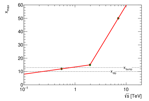
As the measurements were performed at different values of the horizontal axis , some interpolations were however inevitable. The technical aspects of these interpolations were detailed in section 6. Let us illustrate these interpolations by the two panels of Fig. 14. We hope, that these pictures illustrate the model independent nature of our analysis more clearly than the technical description of these interpolations.
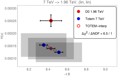
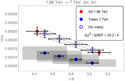
Our final quantification of the Odderon significance is based on a method developed by the PHENIX collaboration in Ref. Adare:2008cg using a specific definition that effectively diagonalizes the covariance matrix. We utilized the measured differential cross-section of elastic scattering and its published covariance matrix at TeV, as measured by TOTEM in Ref. Antchev:2018edk , for a validation of this method. We have adopted the PHENIX method of the diagonalization of the covariance matrix using type A, B and C errors Adare:2008cg .
In its original form, the experimental data that have statistical and systematic errors are compared to a theoretical calculation that is assumed to be a function of the fit parameters. In our final analysis, presented in this Appendix, we adapted the PHENIX method for comparison of a dataset that contains data with errors directly to another dataset, that also contains central data values with errors. So our method is defined without referring to any theoretical model or parameter dependent function. Due to this reason, the most conservative definition described in this Appendix is defined to be symmetric for the exchange of the two datasets.
We classify the experimental errors of a given data set into three different types: (i) type A, point-to-point fluctuating (uncorrelated) systematic and statistical errors, (ii) type B errors that are point-to-point dependent, but 100% correlated systematic errors, and (iii) type C errors, that are point-to-point independent, but fully correlated systematic errors Adare:2008cg to evaluate the significance of correlated data, when the covariance matrix is not publicly available.
Suitably generalizing the method of Ref. Adare:2008cg , that was developed originally for a comparison of a dataset with a theoretical, parametric fit curve, for a comparison of two data sets in this case, where the datasets have type A, B and cancelling type C errors, we obtain the significance of a projection of the data set to data set determined by the following definition:
| (68) | |||||
In this equation, is the type A uncertainty of the data point of the data set in the united acceptance, while is the same for the data set obtained from the dataset by interpolation to point of dataset . Both uncertainties are scaled by a multiplicative factor such that the fractional uncertainty is unchanged under multiplication by a point-to-point varying factor:
| (69) | |||||
| (70) |
In these equations, and stand for the overall correlation coefficient of the -dependent, point-to-point correlated type B to the measured values in data set , of the projected data set . Note that and are independent of the point , while the B-type errors have a point-to-point changing values and in both and in the projected dataset in . For our comparison of scaling functions, where the absolute normalization and type C errors cancel, we have , so have not indicated these terms for the sake of simplicity. For the sake of clarity and to demonstrate the importance of scaling out these type C errors, we have also included Fig. 16. That plot indicates that if the overall correlated, type C errors are added (incorrectly) in quadrature with the point-to-point fluctuating type A errors, the significance of the Odderon signal is decreased from 6.26 to 3.64 .
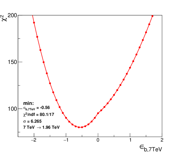
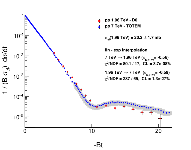
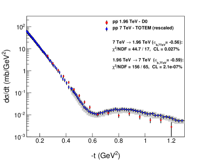
| (GeV) | (mb) | (GeV-2) |
|---|---|---|
| 1960 () | 20.2 [*] | 16.86 Abazov:2012qb |
| 2760 () | 21.8 Nemes:2017gut ; Antchev:2018rec | 17.1 Antchev:2018rec |
| 7000 () | 25.43 Antchev:2013gaa | 19.89 Antchev:2013gaa |
| (mb) | interpolation | direction of projection | NDF | CL (% ) | Significance [] | |
|---|---|---|---|---|---|---|
| 20.2 1.7 | lin-exp | 7 1.96 TeV | 80.1 | 17 | 6.26 |
We have utilized the scaled variance method of ROOT to include the horizontal errors, adding in quadrature to the type A errors also the type A error coming form the type A uncertainty of , denoted as . Similarly, we have added in quadrature to the type B error of the type B uncertainty of , denoted by . Using a notation where may stand for any of or , the errors are given as
| (71) | |||||
| (72) |
where indicates the type error of the value of the vertical error on data point , and it is added in quadrature to , the corresponding vertical error that is associated with the same uncertainty of type originating from the measurement error on the horizontal axis in Eq. (71). The notations and stand for the numerical derivative of the data points at point in the datasets and , respectively.
The errors on the projected data set () are also obtained by a linear-exponential interpolation between the projections of data set 2 () to data set 1 (). Their type A and type B errors, indicated by and are also added in quadrature with the other A or B type of errors. These errors on the interpolated and on the measured values of through equations (71) and (72) provided our most stringent significance estimate for the Odderon effects. We have cross-checked that several variations on the definition, for example the frequently adopted negligence of the horizontal errors and their contribution to the vertical errors through the scaled variance method, or perturbing the central values or the errors of the elastic cross-sections within the allowed limits, may only increase the significance reported in this Appendix.
We have evaluated Eq. (63) as a function of and . However, for the critical test of the projection of the TeV TOTEM data on to that of D0 at TeV, we found that D0 did not publish any error on and cross-checked that the D0 value on contains only type A, uncorrelated statistical and systematic errors only. We also noticed that there are no published type-B errors on the published differential cross-section data of D0 Abazov:2012qb . Hence for the D0 dataset, all the type B errors are zero and as a consequence, we have fixed the correlation coefficient of type B errors to zero for the TeV D0 dataset.
Let us now denote by subscript the projection of the scaling function at TeV measured by TOTEM for reaction to the D0 dataset on elastic scattering at TeV. We found a minimum for within the domain, with the best value of and the lowest value of of Eq. (68) indicated in Fig. 15. Table 6 summarizes the input values and the appropriate references to the utilized elastic cross-section and the nuclear slope . The final and most stringent result of this cross check, corresponding to the lowest values of significance for the Odderon observation is summarized in Table 7. We found that the significance of the Odderon observation in the 7 TeV 1.96 TeV projection is at least , corresponding to a and CL of not larger than %. We notice that all variations of the procedure may only increase this significance. We conclude, that the probability of the Odderon observation in this -channel mode is statistically significant, at least , if the scaling is valid at TeV in the range of . As Fig. 13 indicates that model dependently this range might be smaller, only for TeV, we have also performed several -range stability studies in E.
From the experimental side, a very strong argument to support for the domain of validity of the scaling can be obtained from the observation that the bump/dip ratio is -independent, if the scaling holds up to the bump position, . If the scaling is valid for , we find that
| (73) |
Recent TOTEM data indicate that this ratio is, within the energy range available for TOTEM, and within experimental errors, is indeed independent of Nemes:2019nvj and a diffractive minimum-maximum with an approximately -dependent ratio of , at and TeV, respectively. Apparently, an -independent is within errors a permanent feature of elastic scattering at these energies Nemes:2019nvj . This experimental result supports, that the scaling holds up to at least at energies close to the TeV range. Indeed, at 13 TeV, Nemes:2019nvj , so we expect a similar value of at TeV, too, as this scale is logarithmically close to 2.76 TeV. Due to the observation of a diffractive cone in collisions both at 2.76 and 7.0 TeV Nemes:2019nvj , we expect a similar diffractive cone in elastic scattering at TeV, too, which correspods to . Thus the available experimental data also suggests that the expected domain of validity of scaling at TeV includes the domain. These experimental observations combined with our model independent -range stability studies in E indicate, that in this domain the significance of the Odderon observation is at least 5.0 . This interval physically begins with the “swing", where the differential cross-section of elastic scattering starts to bend below the exponential shape and ends just after the diffractive maximum or “bump", located at . For one of the theoretically expected domains of validity, the limited range, we find that our method provides an Odderon significance of at least 5.3 , as detailed in E. Another theoretical argument is shown in Fig. 27, where the scaling limit of the ReBB model of Ref. Csorgo:2020wmw is shown to describe the experimental data in the whole D0 acceptance, corresponding to the domain of validity of range and a 6.25 Odderon effect. This is one of the indications of the robustness of our results.
For the sake of completeness, we also evaluate the asymmetry parameter from the scaling functions to demonstrate the level of agreement between the experimental data and our full model calculations and also to have a better insight on the magnitude of the scaling violations. In order to measure the size of the Odderon effect, let us define the following asymmetry measure or asymmetry parameter:
| (74) | |||||
| (75) |
If the crossing-odd component of elastic scattering amplitude vanishes at high energies, it implies that . In this case, we find that for TeV. Additionally, if scaling holds for elastic scattering at high energies, then , hence . Indeed, as Fig. 17 indicates, this asymmetry parameter vanishes within experimental errors. There are small systematic deviations that are well described by theoretical model calculations based on the Real Extended Bialas-Bzdak model of Ref. Csorgo:2020wmw . The agreement between the small asymmetries and the theoretical calculations indicates that the scaling violations are under precise theoretical control.
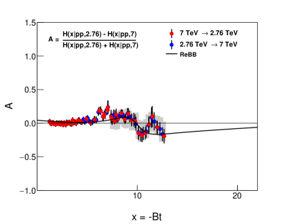
On the other hand, if the scaling holds for elastic scattering and the crossing-odd component of elastic scattering amplitude is not vanishing at high energies, then , hence for TeV. Indeed, as shown in Fig. 18, this asymmetry parameter is significantly different from zero. Similarly to Fig. 17, the solid line in Fig. 18 is the result of a model calculation based on the full version of the Real Extended Bialas-Bzdak model of Ref. Csorgo:2020wmw . The solid line describes the experimental data well, within errors, which indicates that the scaling violations are well under theoretical control in this calculation.
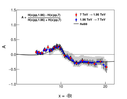
Appendix B Pomeron and Odderon at the TeV energy scale: model independent properties
In this Appendix we discuss some model independent properties of the Pomeron and Odderon that utilize their correspondence with the crossing-even and crossing-odd components of the elastic scattering amplitude at the TeV energies. In the TeV energy range, we identify the crossing-even and crossing-odd components with the Pomeron and the Odderon amplitude, given that the Reggeon contributions in this energy range are generally expected to be negligibly small, as confirmed also by explicit calculations for example in Ref. Broniowski:2018xbg . These results are obtained by a straightforward generalization, from a model dependent to a model independent class, of the Pomeron and Odderon properties obtained in Ref. Csorgo:2020wmw for the Real Extended Bialas-Bzdak model of Ref. Nemes:2015iia .
The proton-proton () as well as the proton-antiproton () elastic scattering amplitudes can always be written as the difference as well as the sum of the the -even and -odd amplitudes, as detailed in Eqs. (14,15). These amplitudes depend on Mandelstam variables and , but we suppress these dependencies in our notation throughout this B.
With the help of the and the scattering amplitudes, the crossing even and the crossing odd components of the elastic scattering amplitude can be expressed as Eqs. (18,19). The and the scattering amplitudes can be evaluated based for example on R. J. Glauber’s theory of multiple diffractive scattering Glauber:1955qq ; Glauber:1970jm ; Glauber:2006gd , and various models of the structures inside the protons. However, in this Appendix we focus on the model-independent properties so we do not specify a model yet. Model dependent calculations are subject of C and D.
The differential elastic cross section is defined by Eq. (2). The elastic, the total and the inelastic cross sections are given by Eqs. (1,5) and Eq. (6), respectively. The real to imaginary ratio is given by Eq. (8), and the nuclear slope parameter is given by the model independent relation of Eq. (4).
These measurable quantities are utilized to characterize experimentally the -dependent elastic scattering amplitudes, discussed above. These quantities can be evaluated for a specific process like elastic or elastic collisions. If we can evaluate the elastic scattering amplitude for both and scattering in the TeV energy range, that straightforwardly yields also the -dependent elastic scattering amplitude also for the Pomeron and the Odderon exchange.
Let us focus on the model independent properties of the crossing-even Pomeron () and for the crossing-odd Odderon () exchange.
The scattering amplitude , for spin independent processes, is related to a Fourier-Bessel transform of the impact parameter dependent elastic scattering amplitudes :
| (76) |
Here, is the modulus of the impact parameter vector , stands for the modulus of the transverse momentum vector and is the is the zeroth order Bessel-function of the first kind. In the considered high energy limit, and in this case the modulus of the transverse momentum transfer is calculated as .
This impact parameter dependent amplitude is constrained by the unitarity of the scattering matrix ,
| (77) |
where is the identity matrix. Its decomposition is , where the matrix is the transition matrix. In terms of , unitarity leads to the relation
| (78) |
which can be rewritten in terms of the impact parameter or dependent amplitude as
| (79) |
where is a non-negative contribution. If the process is completely elastic, this quantity is zero, and the elastic amplitude lies on the Argand circle, while in case there are also inelastic collisions present, the elastic amplitude lies within the Argand circe Block:2006hy . It can be equivalently expressed from the above unitarity relation as
| (80) |
It follows that
| (81) |
as a consequence of unitarity. Thus probabilistic interpretation can be given only to the inelastic scattering and to the sum of the elastic scattering amplitude and the amplitude for propagation without interaction. This is why elastic scattering is a genuine quantum or wave-like process, and this is also the reason why elastic scattering, in contrast to inelastic scattering, has no classical interpretation. Thus is interpreted as the impact parameter and -dependent probability of inelastic scattering.
The elastic scattering amplitude has the unitary form of Eq. (12) as the function of the center-of-mass energy squared and impact parameter . This form is expressed with the help of the opacity (or, eikonal) function, denoted by , which in the general case is a complex valued function.
The imaginary part of determines the real part of the scattering amplitude, while the real part of determines the dominant, imaginary part of the scattering amplitude. Let us introduce with the help of the real part of the complex opacity function as follows:
| (82) |
This leads to Eq. (41).
The shadow profile function is defined with the help of the opacity function, which yields
| (83) |
This relation indicates that is interpreted as the probability of inelastic collisions at a given value of the squared center of mass energy and impact parameter . The inelastic profile function can in general be evaluated with the help of Glauber’s multiple diffraction theory Glauber:1970jm , using various model assumptions, for example the assumptions of Ref. Nemes:2015iia .
The impact parameter dependent elastic scattering amplitudes for elastic and scatterings are given in terms of the complex opacity or eikonal functions . The defining relations are
| (84) | |||||
| (85) |
The explicit expressions for the -even and the -odd components of the impact parameter dependent elastic scattering amplitude are detailed below. These relations are explicit consequences of unitarity and do not depend on model details. However, it is important to note that at the TeV energy range in , the -even exchange corresponds to the Pomeron exchange while the -odd amplitude corresponds to the Odderon exchange, while the corrections due to the exchange of Reggeons or hadronic resonances is smaller than the experimental errors as detailed recently in Ref. Broniowski:2018xbg . Thus, in the TeV energy range, the -matrix unitarity and the dominance of the Pomeron and Odderon amplitudes constrains their form as follows:
It is obvious to note that the Pomeron amplitude given above is crossing-even, while the Odderon amplitude is crossing-odd: and .
Under two assumptions, these relations can be further simplified for a broad class of models as follows.
-
•
i) If the imaginary part of the complex opacity function in elastic and collisions has the same -dependent factor, denoted here in general by , and
-
•
ii) if these imaginary parts of the complex opacity function also include an -dependent but independent prefactor that is a different function in elastic and in collisions,
then these assumptions correspond mathematically to the following relations:
| (86) | |||||
| (87) |
yielding the following simple expressions for the impact parameter dependent elastic and scattering amplitudes
| (88) | |||
| (89) |
These relations can be equivalently rewritten for the Pomeron amplitude, using and as shorthand notations while also suppressing the -dependence of and :
This form of the Pomeron amplitude is explicitly -even, and satisfies unitarity. Thus, if the difference between the opacity parameters for and elastic collisions is small, the Pomeron is predominantly imaginary, with a small real part that is proportional to . Similarly, for the Odderon we have, under the conditions i) and ii), real and imaginary parts of the following amplitude
This form of the Odderon amplitude is explicitly -odd and satisfies unitarity, if the above two assumptions i) and ii) are satisfied, without any further reference to the details of the model. In this class of models, if the difference between the opacity parameters for and elastic collisions becomes vanishingly small, both the real and the imaginary parts of the Odderon amplitude vanish, as they are both proportional to . If this term is non-vanishing, but remains small, the above Odderon amplitude remains predominantly real, with a small, linear in at the leading order, imaginary part.
Appendix C Emergence of the scaling from the Real Extended Bialas-Bzdak model
With the help of the ReBB model of Ref. Nemes:2015iia , we have recently described the and differential cross-sections in a limited kinematic range of TeV and GeV2, in a statistically acceptable manner with CL 0.1 %, as detailed in Ref. Csorgo:2020wmw .
It is important to realize that within the ReBB model, the elastic scattering dependence on comes only through four energy-dependent quantities, as specified recently in Ref. Csorgo:2020wmw . Let us recapitulate the general formulation, for the sake of clarity, denoting the -dependent quantities as , , and :
| (92) |
Similarly, the scattering amplitude of the elastic scattering is found in terms of four energy-dependent quantities, that we denote here for the sake of clarity as , , and :
| (93) |
Here, stands for a symbolic short-hand notation for a function, that indicates how the left hand side of the and scattering amplitude depends on through their -dependent quantities. Among those, , , and correspond to the Gaussian sizes of the constituent quarks, diquarks and their separation in the scattering (anti)protons. These scales are physically expected to be the same in and in elastic collisions.
Indeed, the trends of , and follow, within errors, the same excitation functions in both and collisions, as indicated on panels a, b and c of Fig. 6 of Ref. Csorgo:2020wmw . Due to this reason, let us denoted these – in principle, different – scale parameters with the same symbols in the body of the manuscript, as they are found to be independent of the type of the collision, i.e.
| (94) | |||||
| (95) | |||||
| (96) |
On the other hand, the opacity or dip parameter is different for elastic and reactions: if they were the same too, then the scattering amplitude for and reactions were the same, and correspondingly the differential cross-sections were the same in these reactions, while the experimental results indicate that they are qualitatively different Csorgo:2020wmw . Hence,
| (97) |
The ReBB model Nemes:2015iia provides a statistically acceptable description of the elastic scattering amplitude, both for and elastic scattering, in the kinematic range that extends to at least GeV2 and TeV. For the sake of clarity, let us also note that the -dependence of the Pomeron and Odderon components of the scattering amplitude thus happens through the -dependence of five parameters only. Based on Ref. Csorgo:2020wmw , we write
Here, and are just symbolic short-hand notations that summarize how the left hand sides of the above equations depend on through their -dependent parameters.
As detailed in Ref. Csorgo:2020wmw , within the ReBB model there is a deep connection between the and the dip region. This supports the findings that the recently observed decrease in around 13 TeV, the dip-bump structure in scattering and its absence in scattering are both the consequences of the Odderon contribution. In the ReBB model, this Odderon contribution is encoded in the difference between and . This conclusion is supported also by the detailed calculations of the ratio of the modulus-squared Odderon to Pomeron scattering amplitudes. Thus, if , within the ReBB model it follows that or, equivalently, in the TeV region.
Within the framework of the ReBB model, we have proved in Ref. Csorgo:2020wmw
an interesting Odderon theorem. The weaker, original form of this theorem was formulated
above in Sec. 3 as follows:
Theorem 1
If the differential cross sections differ from that of scattering
at the same value of in a TeV energy domain, then the Odderon contribution to
the scattering amplitude cannot be equal to zero, i.e.
| (100) |
This theorem is model-independently true as it depends only on the general structure of
the theory of elastic scattering. Within the ReBB model, this theorem has been sharpened in Ref. Csorgo:2020wmw as follows:
Theorem 2:
In the framework of the unitary ReBB model, the elastic differential cross sections differ
from that of elastic scattering at the same value of in a TeV energy domain,
if and only if the Odderon contribution to the scattering amplitude is not equal to zero.
This happens if and only if and as a consequence,
if and only if :
In this work, we extend these theorems to the emergence of scaling within the ReBB model,
as follows:
Theorem 3:
In the framework of the unitary ReBB model, the elastic differential cross sections
obey a scaling in a certain kinematic region, if and only if in that region the opacity
parameter is approximately energy independent, and the geometrical
scale parameters evolve with the same -dependent, but radius parameter independent factor .
Thus, the conditions of validity of scaling in elastic collisions, within the framework
of the ReBB model are the simultaneous validity of the following four equations:
| (101) | |||||
| (102) | |||||
| (103) | |||||
| (104) |
where is the same function of for each of , and .
The key point of the proof of Theorem 3 is that is related, for an analytic amplitude, to the variance of the scattering amplitude in the impact parameter space. If this variance depends on the evolution of the scale parameters , and only, as is within the experimental errors a constant, and if these scale parameters all evolve with the same -dependent factor, then the nuclear slope parameter must also scale as
| (105) |
At the same time, the elastic and the differential cross-sections must also scale as
| (106) | |||||
| (107) |
Hence, in such an and , range the scaling, defined by Eq. (54) must hold: and vice versa.
We have cross-checked the scaling properties of the ReBB model at both ISR and LHC energies. At the ISR energies of 23.5 GeV, is not a constant as reviewed recently in Antchev:2017yns , so our Theorem 3 suggests, that the scaling cannot be interpreted in terms of the ReBB model, and in particular we expect that , the bump-to-dip ratio decreases with increasing values of as ref. Antchev:2017yns suggests that is an increasing function of at ISR energies. Thus, the approximate scaling, indicated in Fig. 1 actually is expected to be violated in the dip regions and also perhaps also in the tail region at ISR energies. A more detailed investigation of the scaling violations at ISR energies goes well beyond the scope of this manuscript.
At LHC energies, let us summarize the main results of the ReBB model studies, as given in Ref. Csorgo:2020wmw in greater details. If we do not utilize the validity of the scaling at the LHC energies, we obtain Figs. 16, 17 and 18 of Ref. Csorgo:2020wmw . In these figures a yellow band indicates the uncertainty of the model prediction, without the assumption of the validity of the scaling. Fig. 16 of Ref. Csorgo:2020wmw indicates that the extrapolation without the scaling is rather uncertain in the region of the diffractive shoulder as compared to TeV elastic scattering data and correspondingly, no significant difference is observed in this model comparison at this energy. However, the model allows for the investigation of scaling violations and the extrapolation of data to the LHC energies. As the data do not obey a scaling, their extrapolation to the LHC energies without such a model is not possible: the scaling works only for but not for collisions. Comparing the ReBB model extrapolations of differential cross-sections with TOTEM data on differential cross-sections at TeV, we obtained in Ref. Csorgo:2020wmw an Odderon effect with a significance of 7.12, as indicated on Fig. 17 of Ref. Csorgo:2020wmw . Combining this value with the model dependent results at TeV, the combined significance is hardly reduced, changes only to 7.08 . On the other hand, if we extrapolate data also up to TeV, the significance increases further, to values greater than 10. In practical terms, extrapolating data theoretically up to 7 TeV, we obtain a certainty for the Odderon contribution. The quoted 6.26 model independent significance is thus a safe, model independent lower limit for the observation of a crossing-odd component of elastic and scattering in the TeV energy range.
Appendix D Model-dependent estimation of the range of validity and violations of scaling
In this Appendix, we summarize our model-dependent results on the estimated range of validity of scaling in elastic collisions. We find that this scaling might be extended in from 7 and 8 TeV at LHC down to GeV at RHIC, as detailed below.
The , and parameters of the ReBB model were determined in Ref. Csorgo:2020wmw using both an affine linear and a quadratic dependence on . This allowed us to test if the scale parameters of the ReBB model obey, within one standard deviation, the same energy dependence or not. For the reference point, we have chosen TeV. Fig. 19 indicates that such an affine linear scaled energy dependence of the ReBB model parameters , and by the values of the same parameters at 7 TeV suggests that the one systematic error-bands overlap down to GeV. However, this result does not yet take into account the possible quadratic dependence of these parameters on and it also neglects the correlations between the model parameters. However, the validation of this linear in energy dependence of the factor of the scaling by an explicit calculation failed, indicating that a quadratic extrapolation in is apparently necessary.
Taking into account the possible quadratic in dependence of the excitation function of the ReBB model parameters , and pushes this limit further down to GeV, as demonstrated in Fig. 20. This plot utilizes the parameters of quadratic dependence in as indicated in Fig. 23 of Ref. Csorgo:2020wmw , and collected in Table 3 of that manuscript, but without taking into account the correlations between these model parameters. When we tried to validate such a quadratic in but uncorrelated dependence of the parameter of the scaling, the validation plots did not result in acceptable confidence levels with CL % for , and TeV. Hence we had to take into account the correlations between , and together with their quadratic in behaviour as detailed below.
Our final estimate for the range of the validity of the scaling, in particular, the possible lowest value for the validity of this scaling is based on the quadratic in dependence of the model parameters , and , taking also into account their correlations. This we have studied so that we determined these parameters at 5 different energies, at GeV, as well as at 0.546, 1.96, 2.76 and 7 TeV, and fitted the resulting 5 points with a 3-parameter quadratic formula of . This line is our best estimate for the quadratic energy dependence for these parameters. However, the parameters are correlated so we have repeated these fits by shifting up (or down) by one standard deviation each of these model parameters at each energy and fixed their values, while re-fitting all the other parameters of the ReBB model at the same energy to find their best estimate. This way we perturbed in two different directions four model parameters at five different energies and re-fitted each set with the quadratic in evolution, resulting in 2x4x5 = 40 curves around the central line. The area between these curves is our best estimate for the systematic error band of the energy evolution, that takes into account not only the errors of the ReBB model parameters but also the correlations between the ReBB model parameters at each energy.
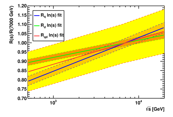
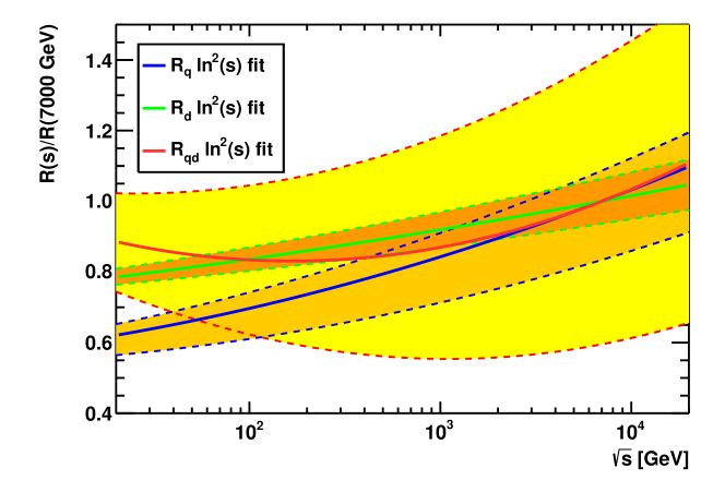
The one systematic error band on the parameter, that takes into account both the quadratic in evolution and the correlations between the model parameters is presented as an orange band in Fig. 21. Similarly, the one systematic error band on the parameter, that takes into account both the quadratic in evolution and the correlations between the model parameters is presented as a darker orange band in Fig. 22. The same error band is shown for the parameter in yellow band in Fig. 23. These error bands are actually overlapping and the region of their overlap determines the domain of validity of the scaling.
The overlaid one systematic error-bands of the scale parameters of the ReBB model are shown in Fig. 24. This figure indicates that from TeV down to GeV these one standard deviation error-bands overlap within one standard deviation. This implies, that one of the necessary conditions for the validity of the scaling in elastic collisions is satisfied in the kinematic range of TeV. The domain of validity of the ReBB model was limited in as well, to GeV2 as detailed in Ref. Csorgo:2020wmw . Thus, this model-dependent study cannot be applied at very low or very high values of and the additional condition for the domain of validity of the scaling, the constancy of the parameter can be cross-checked if experimental data on elastic collisions are becoming available in the lower end of this energy range.
Let us first cross-check if indeed the scaling can be valid in elastic or collisions in such a broad energy range, or not. We have demonstrated that this scaling is violated if we go with energy up to TeV. This is easily understood within the framework of the ReBB model. Condition ii) indicates that one of the necessary condition for the scaling is the constancy, the approximately energy independence of the parameter . In Ref. Csorgo:2020wmw we have shown that within the ReBB model this corresponds to the energy independence of the real to imaginary ratio at , the parameter . The TOTEM Collaboration recently demonstrated that at the top LHC energy of TeV, the parameter starts to decrease significantly Antchev:2017yns . This decrease increases the dip at these energies corresponding to Theorem 2 of Ref. Csorgo:2020wmw and thus the decrease of leads also to a violation of the scaling at the top LHC energies.
At the lower energies, the scaling of elastic collisions imposes a condition also on the differential cross-sections of elastic collisions. Although the value of is not constrained, the scale parameters in and in elastic collisions were found to follow the same trends. Hence, if scaling is valid down to GeV, then the scale parameters of elastic collisions at and TeV have also to follow the common energy dependencies as specified by Eqs. (101,102,103). So the validity of the scaling in elastic collisions constrains the possible shape of elastic collisions as well within the framework of the ReBB model and these constraints can be tested both theoretically and experimentally.
Let us present the tests of the upper limit of the domain of validity in of the scaling on experimental data first.
The test of the validity of the scaling, using elastic data at TeV LHC energy is shown in Fig. 25. The agreement at 2.76 TeV is excellent and needs no comments or explanations. The upper limit of the validity of the scaling, at this TeV can not be determined from this plot, as apparently that is this upper limit is clearly larger, than the upper end of the acceptance in of the TOTEM experiment at this energy.
At TeV, , the upper limit of the domain of the validity of the scaling is investigated in Fig. 26. For collisions, remains the only free fit parameter, except the overall normalization parameters. In this case, the differential cross-sections are constrained, because of the requirement is a prescribed function of and the parameters at TeV are already determined at 7 TeV. As indicated in Fig. 26, these constraints are satisfied with a CL = 0.2 % 0.1 % for the measured data, but only in a rather narrow kinematic region of GeV2.
An important test of the validity of the scaling collisions at the Tevatron energy of TeV is indicated in Fig. 27. In this plot, the model parameters , and are constrained by the scaling. Solid line indicates that one parameter, can be fitted to describe the D0 differential cross-section in the whole acceptance of the D0 experiment in . According to this plot, at the D0 energy of , the domain of the scaling extends to the GeV2 domain, which corresponds to at TeV. In collisions, the other condition of validity of the scaling is that is independent of the energy of the collision in the TeV range, however, for collisions, is a free fit parameter. For collisions, the scaling limit of the ReBB model of Ref. Csorgo:2020wmw describes the D0 data in a statistically acceptable manner, with a CL = 0.7 % , corresponding to an agreement with a , and no significant deviation, an agreement at the 2.69 level.
As the diffractive minimum in is deeper than in if the scaling is valid, the plot also indicates that a signal of Odderon exchange is also present in the ReBB model if extrapolated with the scaling for collisions to TeV. However, some significances are lost, due to two reasons: i) the ReBB model-dependent extrapolations are limited to the GeV2 region, while the model-independent comparisons can be utilized in the whole region; and ii) the comparison is done on the level of the differential cross-sections so the overall correlated, type errors do not cancel. In this case, for the Odderon signal we find a , corresponding to a statistical significance of .
In addition to these experimental tests, that are obtained from fitting measured data with the help of one free parameter, and using the results for the -dependence of the other 3 physical parameters of the ReBB model, , and , we can have a theoretical test as well. This corresponds to the evaluation of the differential cross-section of elastic collisions from both the scaling limit of the ReBB model of refs. Nemes:2015iia ; Csorgo:2020wmw and from the fully fledged version of the same model, that includes also terms that result in scaling violations, and makes the full functions weakly -dependent. Evaluating the error bands from the uncertainty of the model parameters, we can evaluate at a given by determining the domain in , where the two calculations agree within 1 standard deviations of the model parameters. Such a calculation is performed in Fig. 28. This calculation does not allow for a compensation of the modification of the shape by a possible overall normalization factor and so it results in a more stringent upper limit for the domain of the validity of the scaling, at TeV.
Recently, the STAR collaboration measured the differential cross-section of elastic collisions at the center-of-mass energy of GeV Adam:2020ozo . This measurement has resulted in a straight exponential differential cross-section in the range of GeV2. This range is the range where and the conditions of the validity of the scaling are indeed satisfied by this dataset, that is, however, limited to a rather low range. It is thus a very interesting and most important experimental cross-check for the validity of the scaling to push forward the experimental data analysis of elastic collisions at the top RHIC energy of GeV including if possible a larger range extending to the non-exponential domain of as well.
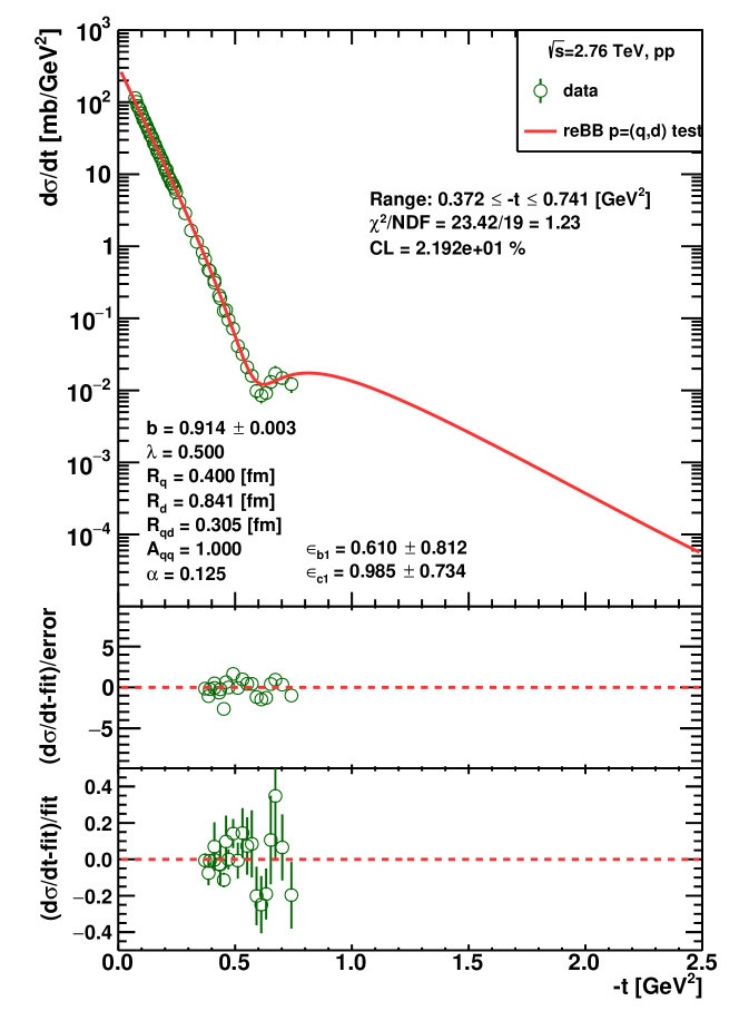
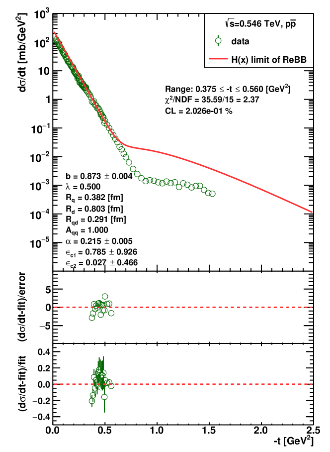
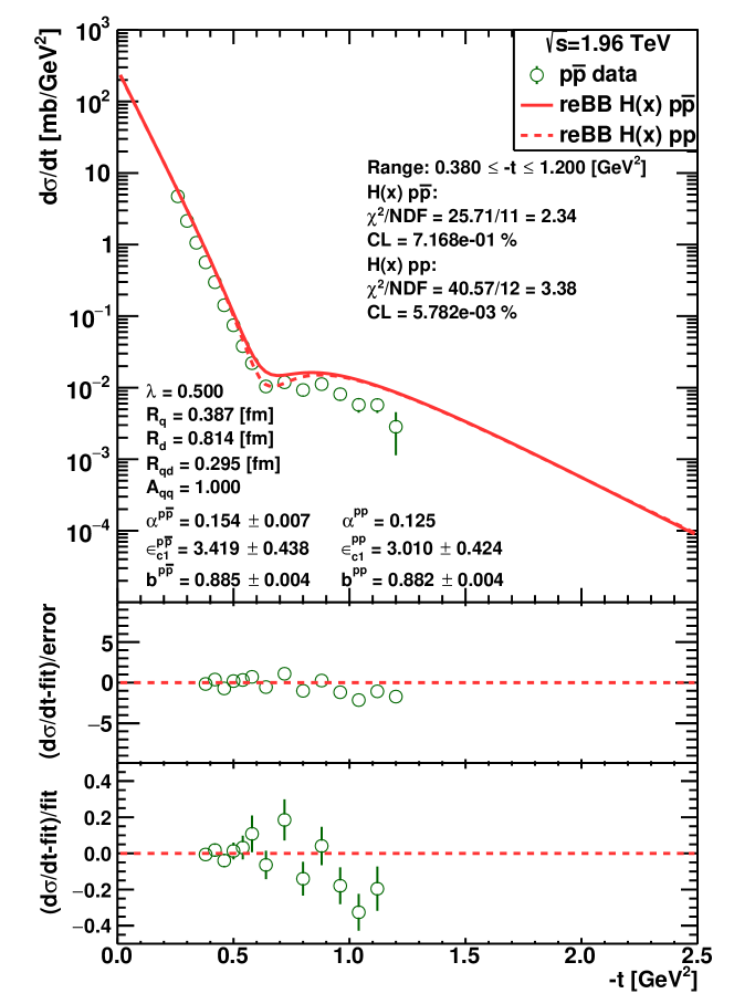
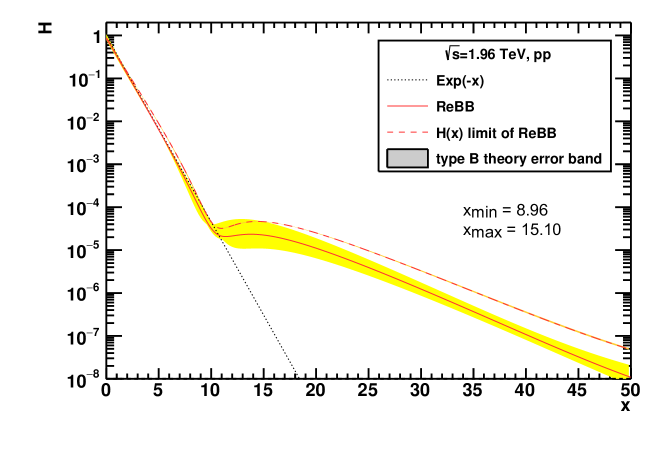
Appendix E Study of the stability of the Odderon signal for the variation of x-range
In this Appendix, we summarize our range stability results. The central topic of this Appendix is the clarification of the role of the correlation between the correlation coefficient and the domain of , over which the or the statistical significance is optimized. This correlation coefficient shifts all the projected datapoints together, up or down, and its best value for all the datapoints is if the scaling function of the densest dataset of TeV is projected to the TeV data. If we fixed this value, and started to limit the -range of comparison by removing 1, 2, 3, 4, 5 and 6 D0 datapoints with the largest values of , we obtain the results summarized in Table 8.
![[Uncaptioned image]](/html/1912.11968/assets/figs/Appendix-E/Table-E-1.png)
In this case of a constant, -range independent , the for all the points and the 6.26 overall significance are both constants, but the partial contributions to the and NDF are -range dependent. Note, that even for the region (left from the dip) we obtain a significant contribution, with a statistical significance of 5.46 . This is seen visually in Fig. 8 as well as on our final comparison plots, Fig. 15 in A.
However, if we applied a more conservative approach, and re-optimized the correlation coefficent to obtain an -range dependent , that minimizes the partial contributions to the in the investigated -range, we obtain the results summarized in Table 9.
![[Uncaptioned image]](/html/1912.11968/assets/figs/Appendix-E/Table-E-2.png)
As shown in Table 9, the correlation coefficient turns out to be strongly -range dependent. The importance of the contribution from large values of can be formulated as follows: if we optimize the correlation coefficient for the range of investigation, the Odderon signal is stable for the removal of the top 1, 2, 3 and 4 D0 datapoints with , as even with the -range dependent minimization of the , the statistical significance of the Odderon observation remains at least 5.33 . However, if we remove 5 or more of the D0 datapoints at large values of , then the remaining D0 data and the scaling function of at TeV can be renormalized to the top of each other. TOTEM data at TeV extend only to the region, where even a 2.5 level, statistically not significant apparent agreement can be reached by totally distorting the value of the correlation coefficient , even if using only the more dense and more precise TOTEM 7 TeV pp data. Orange colored fields indicate that if we apply a local optimalization to the correlation coefficient , this increases the overall significance of the Odderon, if all the datapoints are used. As indicated by the last column of Table 9, these values of the correlation coefficient are gradually becoming rather unreasonable, when all the datapoints are considered. As more and more D0 data points are removed at high , the global statistical significance increases drastically, even above the model-dependent limit of 7.08 , as indicated by the red-colored fields in the rightmost column of the above table. This 7.08 limit corresponds to the combined significance of vs comparisons at both and TeV, as summarized in Table 4 below, and detailed in Ref Csorgo:2020wmw .
If we fully utilize the results of the model dependent analysis of Ref. Csorgo:2020wmw , we find a larger, combined significance of 7.08 as shown in Table 10. This result is obtained by comparing simultaneously the and differential cross-sections at and TeV with the help of the ReBB model. The increased significance is due to the fact that with the help of the same model, the data can also be extrapolated to TeV and result in an overwhelming Odderon signal. Let us stress, that this model dependent significance is obtained even without using the 7 TeV TOTEM dataset, to evaluate the and the Odderon significance and to bridge the energy gap between 2.76 and 1.96 TeV. If the differential cross-section is evaluated and extrapolated also up to 7 TeV with the help of the same ReBB model, the probability of Odderon observation becomes very much larger than a 7.08 effect Csorgo:2020wmw , practically it becomes a certainty.
![[Uncaptioned image]](/html/1912.11968/assets/figs/Appendix-E/Table-E-3.png)
We have made another cross-check and divided the final result of our calculations to four different regions: We have 2 D0 datapoint in Region 0, the diffractive cone with . The remaining 15 D0 datapoints can be divided into 3 regions with 5-5 D0 data points as follows. Region I corresponds to the “swing” region, just to the left of the dip, corresponding to ; Region II, including the dip and the bump, to ; and Region III, the tail corresponds to . We evaluated their partial contributions to our final Odderon significance of 6.26 . For a cross-check we have also evaluated their combined significance and also the contribution of the first two D0 datapoint from the diffractive cone.
The results for a fixed - optimized on all the 17 D0 datapoints - are shown in Table 11. In this case, the greatest partial contribution to the Odderon significance comes from the swing region, the second most important contribution comes from the diffractive interference (dip and bump) region with , and for this value of the correlation coefficient, the tail with has a relatively small contribution.
In contrast, similar results for a regionally optimized correlation coefficient, an -range dependent is shown on Table 12. In this case, the greatest partial contribution to the Odderon significance comes from the diffractive interference (dip and bump) region with , the second most important contribution comes from the swing region, , while the relatively least important contribution comes from the tail with . It is important to recognise, that the 10 D0 datapoints in the swing and diffractive interference region already provide a statistically significant, more than 5 Odderon effect. The interference and the tail together also indicate an Odderon effect, with a significance that is between a 3 and a 5 effect. When all these three regions are combined together, they dominate the final Odderon significance, providing out of the Odderon effect for all x.
It is an intriquing problem if one can determine model independently the region, from where the dominant contribution to the Odderon signal is coming. To reach that goal, we have developed a so called sliding window technique, and determined the minumum size of this sliding window that still provides an Odderon signal on the discovery level of at least 5.0 . Namely, D0 published 17 datapoints. We have taken the first of these datapoints, with varied from 2 to 17, and then locally optimized the correlation coefficients for both projections of TeV and TeV, and determined where the minimum sized sliding window is, wherein the observation of the Odderon is an at least 5 effect. As one picture is worth ten thousand words according to a Chinese word of wisdom, we have summarized our results in Fig. 29. For the sake of clarity, and only on this plot, we have shifted the TOTEM TeV datapoints by their type errors (properly multiplied by the correlation coefficient that minimalized for that given sliding acceptance window) and show only the type A vertical and horizontal errors. Fig. 29 indicates that there are 8 D0 datapoints in the minimal sized sliding acceptance window, where an at least 5 , statistically significant Odderon signal is observed. Thus 9 out of the 17 datapoints can be removed (5 from the tail and 4 points from the diffractive cone region), without destroying the greater than 5 level of the Odderon significance.
![[Uncaptioned image]](/html/1912.11968/assets/figs/Appendix-E/Table-E-4.png)
![[Uncaptioned image]](/html/1912.11968/assets/figs/Appendix-E/Table-E-5.png)
If we take into account the evolution of as a function of , this evolution becomes model dependent, but allows for the estimation of the domain of validity of the scaling law, as detailed in D.
We obtained our model-dependent results within the framework a Glauber-type calculation using the ReBB model of refs. Csorgo:2020wmw ; Nemes:2015iia . This model is validated at TeV in the region Csorgo:2020wmw . According to the calculations of D, the scaling at this 1.96 TeV energy is expected to be valid at least in the kinematic domain. As we cannot estimate reliably the validity of the lower limit of the scaling at low values of x with this model and in addition, in the diffractive cone, and the scaling is expected to hold, the kinematic domain seems to give the worst possible, model dependent limit for the domain of validity of the scaling at 1.96 TeV. As shown on Table 13, this interval corresponds to a significance of at least 3.82 . In this very limited x range, the corresponding best correlation coefficient, - 0.62, is rather close to the best correlation coefficient, -0.56, that minimizes significance for the case of the complete, kinematic domain of all the D0 data, thus for this correlation coefficient, the significance for the kinematic domain is nearly unchanged from 6.27 to 6.28 . If we assume that the lower limit corresponds to the lower limit of the validation of the ReBB model Csorgo:2020wmw , then we find that in the kinematic domain the significance of the Odderon signal is at least 5.3 , as detailed on Table 13. However, we know that in the low region, there is a diffractive cone, where for scattering amplitudes that are analytic at , and for experimental data that are not indicating a non-exponential behaviour at low values of . This is the case for the TeV D0 and for the TeV TOTEM data, so for closing the energy gap between 1.96 and 2.76 TeV, the lower limit of the applicability of the scaling is actually .
If we fully utilize the results of this model dependent analysis we find that the model dependent, combined Odderon significance on prediction versus data at TeV data and prediction versus data at TeV is 7.08 , as shown on Table 10. This increased significance is due to the fact that with the help of the same ReBB model Csorgo:2020wmw , the data can also be extrapolated to the lowest TOTEM energy of TeV and they result in a dominant Odderon signal, as detailed also in Table 10.
In this Appendix, we thus find a hierarchy of the Odderon significances. When we take theoretical modelling into account, we find that the significance of an Odderon observation on elastic collisions at TeV versus elastic collisions at TeV, in the corresponding TOTEM and D0 acceptances, is at least 7.08 . If we do not utilize fully the model dependent information, but use only the theoretical limits for the validity of the scaling at TeV, we find that the Odderon signal is greater than 5 if the scaling is valid in the range of . We cannot reliably estimate the lower limit of the scaling, but demonstrated on available data that in the diffraction cone, is satisfied. We have validated the model of Ref. Csorgo:2020wmw in the range of at 1.96 TeV, and find that this model dependent domain of validity of the scaling extends up to .
The theoretically and model dependently validated range of scaling at TeV, includes the interval , where we find that the Odderon signal is greater than a 5 effect.
We conclude this -range stability investigations as follows:
-
•
Model independently, we find that the significance of the Odderon is greater than in the domain at TeV.
-
•
In our model independent analysis, we relied only on already published D0 and TOTEM datapoints, without relying on preliminary data. We have evaluated the of the Odderon signal using arithmetic operations only (addition, substraction, multiplication, division) but we did not impose any model dependent fits.
-
•
In our model independent analysis, we utilized a newly introduced scaling function, that is not sensitive to the dominant, and overall correlated normalization errors of the differential cross-sections. As a trade-off, the domain of validity of this scaling became an energy dependent interval.
-
•
This scaling function scales out the trivial energy dependencies that appear due to the energy dependence of the elastic cross-section and the nuclear slope parameter .
-
•
Using a model, validated in the domain, we find that the validity in of the scaling at TeV is extending up to . Using published D0 data, and the same model, we validated in Fig. 27 that the scaling at is extending even up to the end of D0 acceptance, to .
-
•
In the very limited interval , we find that the Odderon signal is greater than a 5 effect at TeV.
-
•
Thus the model independent and at least 5 , discovery level Odderon signal is remarkably stable for the variations of the domain of validity of the scaling at TeV.
![[Uncaptioned image]](/html/1912.11968/assets/figs/Appendix-E/Table-E-6.png)
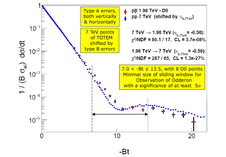
Acknowledgments
We acknowledge inspiring discussions with C. Avila, S. Giani, P. Grannis, W. Guryn, G. Gustafson, L. Jenkovszky, V. A. Khoze, E. Levin, L. Lönnblad, B. Nicolescu, K. Österberg, C. Royon, M. Strikman and M. Šumbera. In particular, we thank our Referees for their valuable comments, suggestions and clarifications and for their suggestion to create an easier-to-read summary of these results, that we have provided in Ref. Csorgo:2020rlb . R.P. is partially supported by the Swedish Research Council grants No. 621-2013-4287 and 2016-05996, by the European Research Council (ERC) under the European Union’s Horizon 2020 research and innovation programme (agreement No. 668679), as well as by the NKFI grant K133046 (Hungary). T. Cs, T. N, I. Sz. and A. S. were partially supported by the NKFIH grants No. FK-123842, FK-123959 and K133046 as well as by the EFOP 3.6.1-16-2016-00001 grant (Hungary). Our collaboration was supported by the framework of COST Action CA15213 THOR: “Theory of hot matter and relativistic heavy-ion collisions".
References
- (1) TOTEM Collaboration, G. Antchev et al., “First measurement of elastic, inelastic and total cross-section at TeV by TOTEM and overview of cross-section data at LHC energies,” Eur. Phys. J. C79 no. 2, (2019) 103, arXiv:1712.06153 [hep-ex].
- (2) TOTEM Collaboration, G. Antchev et al., “First determination of the parameter at TeV – probing the existence of a colourless three-gluon bound state,” arXiv:1812.04732 [hep-ex].
- (3) TOTEM Collaboration, G. Antchev et al., “Elastic differential cross-section measurement at TeV by TOTEM,” Eur. Phys. J. C 79 no. 10, (2019) 861, arXiv:1812.08283 [hep-ex].
- (4) TOTEM Collaboration, G. Antchev et al., “Elastic differential cross-section at and implications on the existence of a colourless C-odd three-gluon compound state,” Eur. Phys. J. C 80 no. 2, (2020) 91, arXiv:1812.08610 [hep-ex].
- (5) A. P. Samokhin and V. A. Petrov, “The Stationary Points and Structure of High-Energy Scattering Amplitude,” Nucl. Phys. A974 (2018) 45–55, arXiv:1708.02879 [hep-ph].
- (6) V. A. Khoze, A. D. Martin, and M. G. Ryskin, “Elastic and diffractive scattering at the LHC,” Phys. Lett. B784 (2018) 192–198, arXiv:1806.05970 [hep-ph].
- (7) L. Lukaszuk and B. Nicolescu, “A Possible interpretation of p p rising total cross-sections,” Lett. Nuovo Cim. 8 (1973) 405–413.
- (8) D0 Collaboration, V. M. Abazov et al., “Measurement of the differential cross section in elastic scattering at TeV,” Phys. Rev. D86 (2012) 012009, arXiv:1206.0687 [hep-ex].
- (9) T. Csörgő, R. Pasechnik, and A. Ster, “Odderon and proton substructure from a model-independent Lévy imaging of elastic and collisions,” Eur. Phys. J. C 79 no. 1, (2019) 62, arXiv:1807.02897 [hep-ph].
- (10) A. Ster, L. Jenkovszky, and T. Csörgő, “Extracting the Odderon from and scattering data,” Phys. Rev. D91 no. 7, (2015) 074018, arXiv:1501.03860 [hep-ph].
- (11) V. P. Gonçalves and P. V. R. G. Silva, “The Phillips–Barger model for the elastic cross section and the Odderon,” Eur. Phys. J. C79 no. 3, (2019) 237, arXiv:1811.12250 [hep-ph].
- (12) V. A. Khoze, A. D. Martin, and M. G. Ryskin, “Elastic proton-proton scattering at 13 TeV,” Phys. Rev. D97 no. 3, (2018) 034019, arXiv:1712.00325 [hep-ph].
- (13) O. Selyugin and J. Cudell, “Odderon, HEGS model and LHC data,” Acta Phys. Polon. Supp. 12 no. 4, (2019) 741, arXiv:1810.11538 [hep-ph].
- (14) M. Broilo, E. G. S. Luna, and M. J. Menon, “Soft Pomerons and the Forward LHC Data,” Phys. Lett. B781 (2018) 616–620, arXiv:1803.07167 [hep-ph].
- (15) M. Broilo, E. G. S. Luna, and M. J. Menon, “Forward Elastic Scattering and Pomeron Models,” Phys. Rev. D98 no. 7, (2018) 074006, arXiv:1807.10337 [hep-ph].
- (16) T. Csörgő, R. Pasechnik, and A. Ster, “Proton structure and hollowness from Lévy imaging of elastic scattering,” Eur. Phys. J. C80 no. 2, (2020) 126, arXiv:1910.08817 [hep-ph].
- (17) S. M. Troshin and N. E. Tyurin, “Implications of the measurements by TOTEM at the LHC,” Mod. Phys. Lett. A33 no. 35, (2018) 1850206, arXiv:1805.05161 [hep-ph].
- (18) E. Gotsman, E. Levin, and I. Potashnikova, “CGC/saturation approach: secondary Reggeons and dependence on energy,” Phys. Lett. B786 (2018) 472–476, arXiv:1807.06459 [hep-ph].
- (19) E. Gotsman, E. Levin, and I. Potashnikova, “A new parton model for the soft interactions at high energies: the Odderon,” arXiv:2003.09155 [hep-ph].
- (20) Y. Hagiwara, Y. Hatta, R. Pasechnik, and J. Zhou, “Spin-dependent Pomeron and Odderon in elastic proton-proton scattering,” Eur. Phys. J. C 80 no. 5, (2020) 427, arXiv:2003.03680 [hep-ph].
- (21) C. Contreras, E. Levin, R. Meneses, and M. Sanhueza, “QCD odderon: Nonlinear evolution in the leading twist,” Phys. Rev. D , arXiv:2004.04445 [hep-ph].
- (22) E. Martynov and B. Nicolescu, “Evidence for maximality of strong interactions from LHC forward data,” Phys. Lett. B786 (2018) 207–211, arXiv:1804.10139 [hep-ph].
- (23) E. Martynov and B. Nicolescu, “Odderon effects in the differential cross-sections at Tevatron and LHC energies,” Eur. Phys. J. C 79 no. 6, (2019) 461, arXiv:1808.08580 [hep-ph].
- (24) Y. M. Shabelski and A. G. Shuvaev, “Real part of scattering amplitude in Additive Quark Model at LHC energies,” Eur. Phys. J. C78 no. 6, (2018) 497, arXiv:1802.02812 [hep-ph].
- (25) G. Pancheri, S. Pacetti, and Y. Srivastava, “Analysis and Implications of precision near-forward TOTEM data,” Phys. Rev. D 99 no. 3, (2019) 034014, arXiv:1811.00499 [hep-ph].
- (26) T. Csörgö, R. Pasechnik, and A. Ster, “Model-Independent Femtoscopic Lévy Imaging for Elastic Proton-Proton Scattering,” Phys. Part. Nucl. 51 no. 3, (2020) 227–231, arXiv:1811.08913 [hep-ph].
- (27) T. Csörgő, R. Pasechnik, and A. Ster, “Lévy imaging of elastic hadron-hadron scattering: Odderon and inner structure of the proton,” Acta Phys. Polon. Supp. 12 no. 4, (2019) 779–785, arXiv:1902.00109 [hep-ph].
- (28) TOTEM Collaboration, G. Antchev et al., “Measurement of proton-proton elastic scattering and total cross-section at = 7 TeV,” EPL 101 no. 2, (2013) 21002.
- (29) W. Broniowski, L. Jenkovszky, E. Ruiz Arriola, and I. Szanyi, “Hollowness in and scattering in a Regge model,” Phys. Rev. D98 no. 7, (2018) 074012, arXiv:1806.04756 [hep-ph].
- (30) F. Nemes, T. Csörgő, and M. Csanád, “Excitation function of elastic pp scattering from a unitarily extended Bialas–Bzdak model,” Int. J. Mod. Phys. A30 no. 14, (2015) 1550076, arXiv:1505.01415 [hep-ph].
- (31) A. Bialas and A. Bzdak, “Constituent quark and diquark properties from small angle proton-proton elastic scattering at high energies,” Acta Phys. Polon. B 38 (2007) 159–168, arXiv:hep-ph/0612038.
- (32) F. Nemes and T. Csörgő, “Detailed Analysis of Elastic Scattering Data in the Quark-Diquark Model of Bialas and Bzdak from GeV to 7 TeV,” Int. J. Mod. Phys. A27 (2012) 1250175, arXiv:1204.5617 [hep-ph].
- (33) T. Csörgő and F. Nemes, “Elastic scattering of protons from GeV to 7 TeV from a generalized Bialas-Bzdak model,” Int. J. Mod. Phys. A29 (2014) 1450019, arXiv:1306.4217 [hep-ph].
- (34) V. Petrov and A. Samokhin, “Is There a Hollow Inside the Proton?,” Int. J. Mod. Phys. Conf. Ser. 47 (2018) 1860097, arXiv:1801.03809 [hep-ph].
- (35) I. M. Dremin and V. A. Nechitailo, “Proton periphery activated by multiparticle dynamics,” Nucl. Phys. A916 (2013) 241–248, arXiv:1306.5384 [hep-ph].
- (36) I. M. Dremin, “Interaction region of high energy protons,” Phys. Usp. 58 no. 1, (2015) 61–70, arXiv:1406.2153 [hep-ph].
- (37) I. M. Dremin and V. A. Nechitailo, “Inelastic profiles of protons at 7 and 13 TeV,” Eur. Phys. J. C78 no. 11, (2018) 913.
- (38) I. Dremin, “Cul-De-Sac of the Spatial Image of Proton Interactions,” MDPI Physics 1 no. 1, (2019) 33–39.
- (39) L. L. Jenkovszky, A. I. Lengyel, and D. I. Lontkovskyi, “The Pomeron and Odderon in elastic, inelastic and total cross sections at the LHC,” Int. J. Mod. Phys. A26 (2011) 4755–4771, arXiv:1105.1202 [hep-ph].
- (40) R. J. N. Phillips and V. D. Barger, “Model independent analysis of the structure in p p scattering,” Phys. Lett. 46B (1973) 412–414.
- (41) P. Lebiedowicz, O. Nachtmann, and A. Szczurek, “Towards a complete study of central exclusive production of pairs in proton-proton collisions within the tensor Pomeron approach,” Phys. Rev. D98 (2018) 014001, arXiv:1804.04706 [hep-ph].
- (42) T. Csörgő and I. Szanyi, “Observation of Odderon Effects at LHC energies – A Real Extended Bialas-Bzdak Model Study,” arXiv:2005.14319 [hep-ph].
- (43) TOTEM Collaboration, T. Csörgő, “Recent Results from the CERN LHC Experiment TOTEM – Implications for Odderon Exchange,” EPJ Web Conf. 206 (2019) 06004, arXiv:1903.06992 [hep-ex].
- (44) M. M. Block, “Hadronic forward scattering: Predictions for the Large Hadron Collider and cosmic rays,” Phys. Rept. 436 (2006) 71–215, arXiv:hep-ph/0606215 [hep-ph].
- (45) D. A. Fagundes and M. J. Menon, “Total Hadronic Cross Section and the Elastic Slope: An Almost Model-Independent Connection,” Nucl. Phys. A880 (2012) 1–11, arXiv:1112.5115 [hep-ph].
- (46) F. J. Nemes, “Elastic and total cross-section measurements by TOTEM: Past and future,” PoS DIS2017 (2018) 059.
- (47) TOTEM Collaboration, G. Antchev et al., “Luminosity-independent measurements of total, elastic and inelastic cross-sections at TeV,” EPL 101 no. 2, (2013) 21004.
- (48) TOTEM Collaboration, G. Antchev et al., “Luminosity-Independent Measurement of the Proton-Proton Total Cross Section at TeV,” Phys. Rev. Lett. 111 no. 1, (2013) 012001.
- (49) S. M. Troshin and N. E. Tyurin, “Reflective scattering from unitarity saturation,” Int. J. Mod. Phys. A22 (2007) 4437–4449, arXiv:hep-ph/0701241 [hep-ph].
- (50) A. Alkin, E. Martynov, O. Kovalenko, and S. M. Troshin, “Impact-parameter analysis of TOTEM data at the LHC: Black disk limit exceeded,” Phys. Rev. D89 no. 9, (2014) 091501, arXiv:1403.8036 [hep-ph].
- (51) S. M. Troshin and N. E. Tyurin, “Effects of the reflective scattering in hadron production at high energies,” Int. J. Mod. Phys. A29 no. 26, (2014) 1450151, arXiv:1408.2650 [hep-ph].
- (52) V. V. Anisovich, V. A. Nikonov, and J. Nyiri, “Hadron collisions at ultrahigh energies: black disk or resonant disk modes?,” Phys. Rev. D90 no. 7, (2014) 074005, arXiv:1408.0692 [hep-ph].
- (53) E. Ruiz Arriola and W. Broniowski, “Proton-proton hollowness at the LHC from inverse scattering,” Phys. Rev. D95 no. 7, (2017) 074030, arXiv:1609.05597 [nucl-th].
- (54) S. M. Troshin and N. E. Tyurin, “The new scattering mode emerging at the LHC?,” Mod. Phys. Lett. A31 no. 13, (2016) 1650079, arXiv:1602.08972 [hep-ph].
- (55) J. L. Albacete and A. Soto-Ontoso, “Hot spots and the hollowness of proton–proton interactions at high energies,” Phys. Lett. B770 (2017) 149–153, arXiv:1605.09176 [hep-ph].
- (56) W. Broniowski and E. Ruiz Arriola, “Hollowness in pp scattering,” Acta Phys. Polon. B48 (2017) 927, arXiv:1704.03271 [hep-ph].
- (57) W. Broniowski and E. Ruiz Arriola, “Hollowness in pp scattering at the LHC,” Acta Phys. Polon. Supp. 10 (2017) 1203, arXiv:1708.00402 [nucl-th].
- (58) S. M. Troshin and N. E. Tyurin, “Experimental signatures of hadron asymptotics at the LHC,” Int. J. Mod. Phys. A32 no. 17, (2017) 1750103, arXiv:1704.00443 [hep-ph].
- (59) I. M. Dremin, “Some new discoveries at colliders,” Usp. Fiz. Nauk 188 no. 4, (2018) 437–445. [Phys. Usp.61,no.4,381(2018)].
- (60) S. D. Campos and V. A. Okorokov, “Hollowness effect and entropy in high energy elastic scattering,” Phys. Scripta 95 no. 9, (2020) 095305, arXiv:1807.02061 [hep-ph].
- (61) J. Dias De Deus, “Geometric Scaling, Multiplicity Distributions and Cross-Sections,” Nucl. Phys. B59 (1973) 231–236.
- (62) A. J. Buras and J. Dias de Deus, “Scaling law for the elastic differential cross-section in p p scattering from geometric scaling,” Nucl. Phys. B71 (1974) 481–492.
- (63) U. Amaldi and K. R. Schubert, “Impact Parameter Interpretation of Proton Proton Scattering from a Critical Review of All ISR Data,” Nucl. Phys. B166 (1980) 301–320.
- (64) TOTEM Collaboration, G. Antchev et al., “Evidence for non-exponential elastic proton–proton differential cross-section at low |t| and =8 TeV by TOTEM,” Nucl. Phys. B 899 (2015) 527–546, arXiv:1503.08111 [hep-ex].
- (65) TOTEM Collaboration, T. Csörgő, “Evidence for Non-Exponential Differential Cross-Section of pp Elastic Scattering at Low and = 8 TeV by TOTEM,” EPJ Web Conf. 120 (2016) 02004, arXiv:1602.00219 [hep-ex].
- (66) T. Csörgő, S. Hegyi, and W. Zajc, “Bose-Einstein correlations for Levy stable source distributions,” Eur. Phys. J. C 36 (2004) 67–78, arXiv:nucl-th/0310042.
- (67) A. Bialas and A. Bzdak, “Wounded quarks and diquarks in heavy ion collisions,” Phys. Lett. B 649 (2007) 263–268, arXiv:nucl-th/0611021. [Erratum: Phys.Lett.B 773, 681–681 (2017)].
- (68) A. Bialas and A. Bzdak, “Wounded quarks and diquarks in high energy collisions,” Phys. Rev. C 77 (2008) 034908, arXiv:0707.3720 [hep-ph].
- (69) A. Bzdak, “The Diquark and elastic pion-proton scattering at high energies,” Acta Phys. Polon. B 38 (2007) 2665–2672, arXiv:hep-ph/0701028.
- (70) T. Csörgő, R. J. Glauber, and F. Nemes, “Elastic proton-proton scattering from ISR to LHC energies, focusing on the dip region,” in International Workshop on Low X Physics. 11, 2013. arXiv:1311.2308 [hep-ph].
- (71) A. K. Kohara, E. Ferreira, T. Kodama, and M. Rangel, “Elastic amplitudes studied with the LHC measurements at 7 and 8 TeV,” Eur. Phys. J. C77 no. 12, (2017) 877, arXiv:1709.05713 [hep-ph].
- (72) J. Kaspar, “Soft diffraction at LHC,” EPJ Web of Conferences 172 (2018) 06005. https://doi.org/10.1051/epjconf/201817206005.
- (73) T. Csörgő, T. Novák, R. Pasechnik, A. Ster, and I. Szanyi, “Scaling of high-energy elastic scattering and the observation of Odderon,” arXiv:2004.07318 [hep-ph].
- (74) TOTEM Collaboration, G. Antchev et al., “Proton-proton elastic scattering at the LHC energy of s** (1/2) = 7-TeV,” EPL 95 no. 4, (2011) 41001, arXiv:1110.1385 [hep-ex].
- (75) PHENIX Collaboration, A. Adare et al., “Quantitative Constraints on the Opacity of Hot Partonic Matter from Semi-Inclusive Single High Transverse Momentum Pion Suppression in Au+Au collisions at s(NN)**(1/2) = 200-GeV,” Phys. Rev. C 77 (2008) 064907, arXiv:0801.1665 [nucl-ex].
- (76) Particle Data Group Collaboration, M. Tanabashi et al., “Review of Particle Physics,” Phys. Rev. D98 no. 3, (2018) 030001.
- (77) I. Szanyi, L. Jenkovszky, R. Schicker, and V. Svintozelskyi, “Pomeron/glueball and odderon/oddball trajectories,” Nucl. Phys. A 998 (2020) 121728, arXiv:1910.02494 [hep-ph].
- (78) W. Czyz and L. C. Maximon, “High-energy, small angle elastic scattering of strongly interacting composite particles,” Annals Phys. 52 (1969) 59–121.
- (79) H. G. Dosch, C. Ewerz, and V. Schatz, “The Odderon in high-energy elastic pp scattering,” Eur. Phys. J. C 24 (2002) 561–571, arXiv:hep-ph/0201294.
- (80) TOTEM Collaboration, F. J. Nemes, “Elastic and Total Cross-Section Measurements by TOTEM,” PoS DIS2019 (2019) 065.
- (81) STAR Collaboration, J. Adam et al., “Results on total and elastic cross sections in proton–proton collisions at = 200 GeV,” Phys. Lett. B 808 (2020) 135663, arXiv:2003.12136 [hep-ex].
- (82) R. J. Glauber, “Cross-sections in deuterium at high-energies,” Phys. Rev. 100 (1955) 242–248.
- (83) R. J. Glauber and G. Matthiae, “High-energy scattering of protons by nuclei,” Nucl. Phys. B 21 (1970) 135–157.
- (84) R. J. Glauber, “Quantum Optics and Heavy Ion Physics,” Nucl. Phys. A 774 (2006) 3–13, arXiv:nucl-th/0604021.