Non-Cooperative Game Theory Based Rate
Adaptation for Dynamic Video Streaming over
HTTP

Abstract

Dynamic Adaptive Streaming over HTTP (DASH) has demonstrated to be an emerging and promising multimedia streaming technique, owing to its capability of dealing with the variability of networks. Rate adaptation mechanism, a challenging and open issue, plays an important role in DASH based systems since it affects Quality of Experience (QoE) of users, network utilization, etc. In this paper, based on non-cooperative game theory, we propose a novel algorithm to optimally allocate the limited export bandwidth of the server to multi-users to maximize their QoE with fairness guaranteed. The proposed algorithm is proxy-free. Specifically, a novel user QoE model is derived by taking a variety of factors into account, like the received video quality, the reference buffer length, and user accumulated buffer lengths, etc. Then, the bandwidth competing problem is formulated as a non-cooperation game with the existence of Nash Equilibrium that is theoretically proven. Finally, a distributed iterative algorithm with stability analysis is proposed to find the Nash Equilibrium. Compared with state-of-the-art methods, extensive experimental results in terms of both simulated and realistic networking scenarios demonstrate that the proposed algorithm can produce higher QoE, and the actual buffer lengths of all users keep nearly optimal states, i.e., moving around the reference buffer all the time. Besides, the proposed algorithm produces no playback interruption.

1 Introduction

Nowadays, with the increase of Internet bandwidth and the tremendous growth of web platforms, Hypertext Transfer Protocol (HTTP) streaming has become a cost-effective method for multimedia delivery [1][2]. Dynamic Adaptive Streaming over HTTP (DASH) is a typical HTTP based multimedia delivery standard that can transmit multimedia content adaptively between multimedia servers and users with a limited and varied network bandwidth [3]. Fig. 1 illustrates a typical DASH-based video delivery system. In this system, the media content (e.g., videos or audios) is first divided into multiple segments (or chunks) [4] with the same display time. Each segment is then encoded/transcoded with different bitrates (corresponding to different quality levels). At the same time, the server generates a Media Presentation Description (MPD) file that records the information of the available video content, e.g., URL addresses, segment lengths, quality levels, resolutions, etc. The users first download the MPD file from the server using HTTP protocol, and then request segments with different quality levels to adapt to the bandwidth variation. The main advantage of DASH is that it can achieve bandwidth adaptation and reduce the number of playback interruptions under fluctuating network conditions [5]. An effective rate adaptation algorithm is necessary in a DASH system, with which the DASH user can adaptively request video segments with different bitrates based on the network condition and its buffer length. However, this challenging issue is not specified in the DASH standard. Without an effective rate adaptation algorithm, the DASH user might suffer from frequent interruptions. Moreover, recent studies show that the DASH user’s selfish behavior (i.e., making requests without considering other users sharing the network resources) will result in network underutilization (or congestion), fluctuating and unfair throughout allocation [6]. This paper aims to develop an effective rate adaptation algorithm to address the above issues.

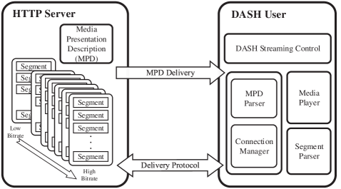
Figure 1: DASH system architecture.

Many rate adaptation methods have been proposed (see Section II). However, most of them optimize the HTTP streaming of multiple DASH users sharing the same network resources separately, regardless of the influence between each other; thus, user fairness cannot be well guaranteed. In contrast, the proposed rate adaptation algorithm optimizes the HTTP streaming of multiple DASH users simultaneously who compete for higher quality video segments from a single server with a limited export bandwidth.

As a branch of game theory, the non-cooperative game theory [7] can resolve the conflicts among interacting players involved in a certain game, in which each player behaves selfishly to optimize its own profit usually quantified as an objective function. The non-cooperative game can provide meaningful solutions for many applications where the interaction among several players is negligible and centralized approaches are not suitable [8][9]. The typical application of a non-cooperative game is the oligopoly market problem in economics, in which all corporations compete for market share of the same commodity in order to maximize their own profits [10], and the market share of each corporation tends to be stable and reaches Nash Equilibrium.

In this paper, we consider formulating the rate adaptation problem for improving user QoE, as well as preserving user fairness, as a non-cooperative game in which DASH users try to consume the limited export bandwidth of the server as much as possible to maximize their profits (i.e., QoE). The optimal bitrate that produces the optimal QoE can be obtained when the Nash Equilibrium of the contradiction problem is achieved. More specifically, the proposed non-cooperative game theory based rate adaptation algorithm determines the requested bitrate for a DASH user based on both the local information (e.g., the requested bitrate of the last segment, reference buffer length, and current buffer length) and the global payoff variation information obtained from the server. Each user can gradually adapt the requested bitrate to convergence. The bitrate’s convergence speed is controlled by the learning rate. Note that there is a limitation that additional HTTP sessions between users and servers are needed in the proposed method, which may reduce the transmission efficiency of the streaming system. Even so, extensive experimental results demonstrate that the proposed algorithm can produce higher QoE, while the actual buffer lengths of all users move around the reference buffer all the time when compared with state-of-the-art algorithms. Moreover, the proposed algorithm is proxy-free and playback interruption-free. To the best of our knowledge, this is the first time to address the DASH rate adaptation problem using the non-cooperative game theory. The major contributions of this paper are summarized as follows.

• We formulated the rate adaptation problem as a non-cooperative game with the existence of the Nash Equilibrium that is theoretically proven. The proposed rate adaptation algorithm optimizes streaming for multiple DASH users simultaneously to guarantee their fairness and improve their QoE.

• We proposed a novel QoE model for the DASH users by taking the current buffer length, reference buffer length, and video quality into account.

• We designed an efficient distributed iterative algorithm to obtain the Nash Equilibrium of the game by additional HTTP sessions between the server and users, the stability of which is theoretically analyzed.

The rest of this paper is organized as follows. In Section II, the related work on rate adaptation methods for DASH is presented. In Section III, a user QoE model is proposed, and the corresponding non-cooperative game is formulated. Besides that, the existence of Nash Equilibrium and the stability of the non-cooperative game are also demonstrated. Simulation and realistic experimental results are given in Section IV and V, respectively. Finally, Section VI concludes the paper and discusses the limitations of the proposed method.

2 Related Work

In order to adapt to the varying bandwidths, a straightforward method is to estimate the bandwidth or throughput of the transmission link. Thang et al. [11] proposed a channel throughput estimation-based adaptive request method to deal with short-term bandwidth fluctuations and stabilize the bitrates of segments. Romero [12] developed a Java client for HTTP streaming on the Android platform and proposed a smoothed throughput estimation method to cope with short-term fluctuations. But the user’s buffer length (evaluated by remaining playback time) has not been considered. In [13], a round-trip time and previous values of the instant throughput based throughput estimation method is proposed for adaptive streaming so as to stabilize both the bitrates of segments and the buffer length of users. Liu et al. [14] developed a throughput estimation based rate adaptation method by using the ratio of the expected segment fetch time (ESFT) and the measured segment fetch time. However, in practical applications, since bandwidth and throughput are affected by a lot of factors, it is a non-trivial task to estimate them accurately. Huang et al. [15] showed that inaccurate throughput estimation at the user side can cause the degeneration of the video quality. Recently, Mao et al. [16] proposed a deep reinforcement learning based rate adaptation algorithm by accurately estimating the channel throughput accurately.

Besides, in order to improve the QoE [17][18] of users directly, some researchers proposed dynamic bitrate selection methods based on QoE maximization [19]-[22]. Zhang et al. [19] proposed a buffer management-based QoE model for HTTP adaptive bitrate streaming and formulated the adaptive request mechanisms as a constrained convex optimization problem which is then solved by the Lagrange multiplier method. Gheibi et al. [20] proposed a QoE metric by considering the probability of interruption in media playback and the number of initial buffered packets (initial waiting time) for streaming media applications. However, QoE is not only influenced by buffer length, but also by the requested bitrate and bitrate switching frequency, etc. Xu et al. [21] modeled the user QoE as a combination of bitrate, starvation probability of playback buffer, and continuous playback time, and they proposed two bitrate switching algorithms based on the channel variation and buffer length. Rodríguez et al. [22] proposed a non-reference QoE metric for DASH by taking initial buffer delay, temporal playback interruptions, and video resolution changes into account. In addition, a Markov decision-based rate adaptation scheme for DASH aiming to maximize the user QoE under time-varying channel conditions was proposed by Zhou et al. [23] in which the video quality level, bitrate switching frequency and amplitude, buffer length, etc. are considered comprehensively. Similarly, Martín et al. [24] proposed a Q-Learning-based bitrate request method to efficiently control the selection of the segment quality by diminishing the quality switches and the occurrence of playback interruption. Bokani et al. [25] proposed another Markov Decision Process-based rate adaptation method based on Q-Learning to gradually learn the optimal decisions in order to avoid playback interruption, which has been found as the most important factor affecting user QoE.

It is worth noting that all of the abovementioned methods are designed based on the assumption that multiple DASH users make their rate adaptation decisions separately. In practical applications, it is more common that multi-users request multimedia content simultaneously from a single server or a relay server of a cell. Since the export bandwidth of the server is limited, a natural problem concerns how to allocate the limited bandwidth jointly to users so as to improve the performance of the whole system, especially to guarantee the fairness of multi-users. In [26], Jiang et al. proposed an optimized bandwidth estimator based on the mean of the previous bandwidths for multi-users to increase bandwidth utilization and stabilize the buffer lengths of multi-users. Li et al. [27] demonstrated that the discrete nature of the video bitrates leads to video bitrate oscillation that negatively affects the video viewing experience and presented a probe-and-adapt bandwidth estimation approach to further increase the bandwidth utilization and stabilize the requested video bitrates of multi-users. Essaili et al. [28] proposed QoE-maximization based traffic and resource management in a mobile network for multi-user adaptive HTTP streaming. However, a proxy is needed to intercept and rewrite the user HTTP requests in this method, which increases the system’s complexity and the channel information for each user is based on the average channel statistics in the previous second that may not be accurate enough.

3 Proposed Rate Adaptation Algorithm

As shown in Fig. 2, in a DASH-based video delivery system, multi-users compete the limited export bandwidth of the server, and the information (i.e., the requested bitrate of the last segment and the current buffer length) of users is unknown by each other. The DASH users first send their current buffer lengths to the server, and then request video segments based on the payoff variation information that is calculated by the server based on the server export bandwidth and the buffer information of each user. We formulate the rate adaptation algorithm into a non-cooperative game as follows.

The players in the game are the DASH users. The strategy of each player is the requested bitrate (denoted by $r_{i}$ for the $i$-th user). The payoff or profit for the $i$-th user (denoted by $U_{i}$) is its QoE determined by the requested video and accumulated buffer. The commodity of the competition is the video segments encoded into different bitrates. The solution of this game is Nash Equilibrium. Let $G=\{I,\{\mathbf{R}_{i}\},\{U_{i}(\cdot)\}\}$ denote the non-cooperative rate adaptation game where $I=\{1,2,\cdots,N\}$ is the index set for the users in the DASH system, and $\mathbf{R}_{i}$ and $U_{i}(\cdot)$ are the strategy space and utility function of the $i$-th user, respectively. Each user determines the required bitrate $r_{i}$ such that $r_{i}\in\mathbf{R}_{i}$. Let the rate vector $\mathbf{r}=\{r_{1},\cdots,r_{i},\cdots,r_{N}\}$ denote the outcome of the game in terms of the requested bitrates of all users. The resulting utility for the $i$-th user is $U_{i}(\mathbf{r})$. We will occasionally use $U_{i}(r_{i},\mathbf{r}_{-i})$ to replace $U_{i}(\mathbf{r})$ to indicate the dependence among DASH users, where $\mathbf{r}_{-i}$ denotes the vector that consists of elements of $\mathbf{r}$ without the $i$-th element, i.e., $\mathbf{r}_{-i}=\{r_{1},\cdots,r_{i-1},r_{i+1},\cdots,r_{N}\}$.

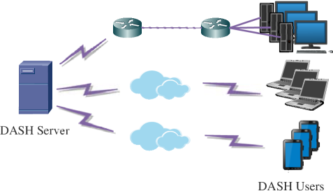
Figure 2: Scenario for adaptive HTTP video delivery.

In the following subsections, we first propose a novel QoE model for DASH users by taking the current buffer length, reference buffer length, and video quality into account. Then, the existence of Nash Equilibrium of the non-cooperative game is theoretically proven. Finally, a distributed iterative algorithm with stability analysis is proposed to find the Nash Equilibrium.

3.1 Modeling of DASH User QoE

In a DASH based video delivery system, the user QoE depends on both the qualities of received video segments and playback interruptions.

1) Video quality: The video quality is directly determined by the bitrate of the requested video.

Although there are a lot of video quality-bitrate models, most of them can be uniformly represented as a logarithmic function of bitrate [29], i.e.,

$$q_{i}(r_{i})=\alpha_{i}\log(1+\beta_{i}r_{i}),$$ (1)

where $q_{i}$ is the quality of the received video segment measured in peak-signal-noise-ratio (PSNR), structure similarity index metric (SSIM) [30], etc., and $\alpha_{i}$ and $\beta_{i}$ are parameters depending on video content. Therefore, without loss of generality, Eq. (1) is used to evaluate the quality of received video segments in the proposed QoE model.

2) Playback interruption: We evaluate the influence of playback interruptions on user QoEs by explicitly modeling the relationship between the estimated buffer length and requested video bitrate. Usually, for the $i$-th user, the buffer variation can be calculated as the difference between the cumulated buffer length (i.e., the remaining video playback time) caused by the downloaded video segment and the consumed buffer length caused by the played video content during the download time [19][31], i.e.,

$$\Delta b_{i}(r_{i})=T-T\cdot{r_{i}/B_{W}^{i}},$$ (2)

where $\Delta b_{i}(r_{i})$ is the buffer variation caused by the requested video bitrate $r_{i}$, $T$ is the length of a video segment, and $B_{W}^{i}$ is the available channel bandwidth of the $i$-th user. Unfortunately, as aforementioned, the channel state of each user is unknown, resulting in Eq. (2) being worthless. But the export bandwidth of the server is known to users. When the summation of the requested video bitrates of all users is larger than the export bandwidth of the server, the download time of all users will increase since the throughput of the system increases.

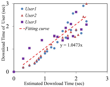
Figure 3: Illustration of the relationship between the actual download time and estimated download time using $T\cdot\sum\nolimits_{j=1}^{N}{r_{j}/B_{W}}$ of each user. Here, three users with varied channel throughputs compete the fixed export bandwidth of a server, and the correlation coefficient is 0.8658.

Therefore, we use the total requested video bitrates of all the users over the export bandwidth of the server to estimate the download time for each user, and the average buffer variation of all users in the system is

$$\Delta b(\mathbf{r})=T-\omega\cdot T\cdot\sum\nolimits_{i=1}^{N}{r_{i}/B_{W}},$$ (3)

where $\omega$ is a coefficient, and $B_{W}$ is the export bandwidth of a server. Such a simple approximation can facilitate the following theoretical analysis with reasonable accuracy. For a single user, the relationship between the actual download time and the estimated download time may not exactly be linear, as shown in ”User1”, ”User2”, and ”User3” in Fig. 3. But for all three users, the overall relationship between the actual download time and estimated download time of all the users can be modeled using a proportional function with the correlation coefficient of 0.8658.

Furthermore, after the current video segment was downloaded, the estimated buffer length of the $i$-th user considering other users denoted as $b_{i}^{est}(r_{i},\mathbf{r}_{-i})$ can be derived by integrating $\Delta b(\mathbf{r})$ over $r_{i}$:

$$\begin{split}&b_{i}^{est}(r_{i},\mathbf{r}_{-i})\\ &=\int\Delta b(\mathbf{r}){\rm d}r_{i}\\ &=T\cdot r_{i}-\omega\cdot T\cdot\left(\frac{1}{2}r_{i}^{2}+r_{i}\sum\nolimits_{\begin{subarray}{c}j=1\\ j\neq i\end{subarray}}^{N}r_{j}\right)/B_{W}+b_{0}\\ &=\Phi(r_{i})-\omega\cdot\Psi(\mathbf{r})+b_{0},\end{split}$$ (4)

where $b_{0}$ is a constant, denoting the initial average buffer length of all the users, $\Phi(r_{i})=T\cdot r_{i}$ is the benefit gained from accumulated buffer, and $\Psi(\mathbf{r})=T\cdot\left(\frac{1}{2}r_{i}^{2}+r_{i}\sum\nolimits_{\begin{subarray}{c}j=1\\ j\neq i\end{subarray}}^{N}r_{j}\right)/B_{W}$ represents the system penalty (buffer consumption) caused by the requested bitrates of all the users.

In order to ensure the buffer is equipped with an optimal state, i.e., the buffer length should be kept within a certain reference level, an adjustment factor (denoted as $A_{f}$) is adopted to modify the revenue function $\Phi(r_{i})$, i.e.,

$$\Phi^{\prime}(r_{i})=A_{f}\cdot\Phi(r_{i})=A_{f}\cdot T\cdot r_{i}.$$ (5)

Considering that a larger (resp. smaller) $b_{curr}$ indicates more aggressive (resp. defensive) behaviors in requesting video segments, $A_{f}$ is defined as a monotonically increasing function of the difference between the current buffer length $b_{curr}$ and the reference buffer length $b_{ref}$ [31]:

$$A_{f}=2\cdot\frac{e^{p(b_{curr}-b_{ref}})}{1+e^{p(b_{curr}-b_{ref})}},$$ (6)

where $p>0$ is a constant, $b_{ref}$ is the predefined reference buffer length, and $b_{curr}$ is the current known buffer length before the video segment was downloaded for a certain user, respectively. The difference between $b_{ref}$ and $b_{curr}$ is an indicator to control the requested bitrates. When $b_{curr}>b_{ref}$, $A_{f}$ is larger than 1, it indicates that the previously received video quality may be low. Then, the bitrates requested by users will be increased to achieve the optimal utility. When $b_{curr}<b_{ref}$, $A_{f}$ is smaller than 1. This indicates that the probability of playback interruption is large. Then, the bitrates requested by users will be decreased to achieve the optimal utility.

Accordingly, the estimated buffer of the $i$-th user with respect to all the other users can be rewritten as

$$\begin{split}&b_{i}^{est}(r_{i},\mathbf{r}_{-i})\\ &=\Phi^{\prime}(r_{i})-\omega\cdot\Psi(\mathbf{r})+b_{0}\\ &=2\cdot\frac{e^{p(b_{curr}-b_{ref})}}{1+e^{p(b_{curr}-b_{ref})}}\cdot T\cdot r_{i}\\ &-\omega\cdot T\cdot\left(\frac{1}{2}r_{i}^{2}+r_{i}\sum\nolimits_{\begin{subarray}{c}j=1\\ j\neq i\end{subarray}}^{N}r_{j}\right)/B_{W}+b_{0}.\end{split}$$ (7)

Finally, we define the utility function of user $i$ that considers the influence on other DASH users sharing the same network resources as the linear combination of the quality function in (1) and the buffer function in (7), i.e.,

$$\begin{split}&U_{i}(r_{i},\mathbf{r}_{-i})\\ &=q_{i}(r_{i})+\mu\cdot b_{i}^{est}(r_{i},\mathbf{r}_{-i})\\ &=\alpha_{i}\log(1+\beta_{i}r_{i})+\mu\left(2\cdot\frac{e^{p(b_{curr}-b_{ref})}}{1+e^{p(b_{curr}-b_{ref})}}\cdot T\cdot r_{i}\right)\\ &-\mu\cdot\omega\cdot T\cdot\left(\frac{1}{2}r_{i}^{2}+r_{i}\sum\nolimits_{\begin{subarray}{c}j=1\\ j\neq i\end{subarray}}^{N}r_{j}\right)/B_{W}+\mu\cdot b_{0}\\ &=\alpha_{i}\log(1+\beta_{i}r_{i})+\mu\left(2\cdot\frac{e^{p(b_{curr}-b_{ref})}}{1+e^{p(b_{curr}-b_{ref})}}\cdot T\cdot r_{i}\right)\\ &-\nu\cdot T\cdot\left(\frac{1}{2}r_{i}^{2}+r_{i}\sum\nolimits_{\begin{subarray}{c}j=1\\ j\neq i\end{subarray}}^{N}r_{j}\right)/B_{W}+\mu\cdot b_{0},\end{split}$$ (8)

where $\mu>0$ is a weight to balance the two parts, and $\nu=\mu\cdot\omega$.

3.2 Proof of the Existence of Nash Equilibrium

The Nash Equilibrium of a game is a strategy profile with the property in which no player can increase its utility by choosing a different action when the other players’ actions are given [32]. A Nash Equilibrium exists for a game $G$ if the following two conditions are met:

a) the strategy space $\mathbf{R}_{i}$ is a non-empty, convex, and compact subset of Euclidean space $\mathbf{R}^{N}$;

b) the utility $U_{i}(\mathbf{r})$ is continuous in $\mathbf{r}$ and (at least) quasi-concave in $r_{i}$.

For the proposed non-cooperative game, the strategy space is composed of the user requested bitrates with the range of $[0,r^{max}]$, where $r^{max}$ is the maximum requested video bitrate of the $i$-th user. Thereby, there is no doubt that $\mathbf{R}_{i}$ is a non-empty and compact subset of Euclidean space $\mathbf{R}^{N}$. According to the definition of the convex set [33], for any $r_{x},r_{y}\in\mathbf{R}_{i}$ and any $\zeta$ with $0\leq\zeta\leq 1$, we have $0\leq\zeta r_{x}\leq\zeta r^{max}$ and $0\leq(1-\zeta)r_{y}\leq(1-\zeta)r^{max}$. Then, we can get $0\leq\zeta r_{x}+(1-\zeta)r_{y}\leq r^{max}$. Therefore, $\zeta r_{x}+(1-\zeta)r_{y}\in\mathbf{R}_{i}$, indicating $\mathbf{R}_{i}$ is a convex set. Thus, condition a) is satisfied. For the utility function in (8), it is obviously a continuous function in terms of $\mathbf{r}$. Besides, the second derivatives of $U_{i}(\mathbf{r})$ with respect to all the $r_{i}$ are

$$\begin{cases}\frac{\partial^{2}U_{i}}{\partial r_{i}^{2}}=-\frac{\alpha\beta^{2}}{(1+\beta r_{i})^{2}}-\frac{\nu\cdot T}{B_{W}},\\ \frac{\partial^{2}U_{i}}{\partial r_{i}\partial r_{j}}=-\frac{\nu\cdot T}{B_{W}}|_{i\neq j},\end{cases}$$ (9)

which are negative because $\alpha$, $\beta$, $\nu$, $T$, and $B_{W}$ are non-negative. Accordingly, the utility $U_{i}(\mathbf{r})$ is a strictly concave function of $r_{i}$ (for all $i$) [33]. Therefore, there must exist a Nash Equilibrium in the proposed rate adaptation game.

For a non-cooperative game, the Nash Equilibrium can be achieved by jointly maximizing the utility functions of all players, i.e., the corresponding best response function of a player is defined as the strategy of the player with those of other players fixed:

$$\mathbf{B}_{i}(\mathbf{r}_{-i})=\arg\max_{r_{i}\in\mathbf{R}_{i}}U_{i}(r_{i},\mathbf{r}_{-i}).$$ (10)

When the Nash Equilibrium is achieved, the strategies of all players can be represented as $\mathbf{r}^{\ast}=\{r_{1}^{\ast},r_{2}^{\ast},\cdots,r_{N}^{\ast}\}$, where $r_{i}^{\ast}=\mathbf{B}_{i}(\mathbf{r}_{-i}^{\ast})$ is the optimal strategy of the $i$-th user and $\mathbf{r}_{-i}^{\ast}=\{r_{1}^{\ast},\cdots,r_{i-1}^{\ast},r_{i+1}^{\ast},\cdots,r_{N}^{\ast},\}$ is the set of the Nash Equilibrium of all users except user $i$.

3.3 Distributed Iterative Algorithm for Nash Equilibrium

Theoretically, the Nash Equilibrium can be obtained by solving the following equations:

$$\frac{\partial U_{i}(\mathbf{r})}{\partial r_{i}}= \frac{\alpha_{i}\beta_{i}}{1+\beta_{i}r_{i}}+\mu\cdot T\cdot\frac{2e^{p(b_{curr}-b_{ref})}}{1+e^{p(b_{curr}-b_{ref})}}$$ (11)

$$-\nu\cdot T\cdot\frac{\sum\nolimits^{N}_{j=1}r_{j}}{B_{W}}=0,\quad\forall i.$$

Taking a DASH system with only 2 users as an example, we have,

$$\begin{cases}\frac{Z_{1,1}}{1+\beta_{1}r_{1}}+Z_{2,1}-Z_{3}(r_{1}+r_{2})=0,\\ \frac{Z_{1,2}}{1+\beta_{2}r_{2}}+Z_{2,2}-Z_{3}(r_{1}+r_{2})=0,\end{cases}$$ (12)

where

$$\begin{cases}Z_{1,1}=\alpha_{1}\beta_{1},Z_{2,1}=\mu\cdot T\cdot\frac{2e^{p(b_{curr,1}-b_{ref})}}{1+e^{p(b_{curr,1}-b_{ref})}},\\ Z_{1,2}=\alpha_{2}\beta_{2},Z_{2,2}=\mu\cdot T\cdot\frac{2e^{p(b_{curr,2}-b_{ref})}}{1+e^{p(b_{curr,2}-b_{ref})}},\\ Z_{3}=\nu\cdot T/B_{W}.\end{cases}$$ (13)

Assume the two users request the same video and have the same channel condition (i.e., two identical users), we have $Z_{1,1}=Z_{1,2}=Z_{1}$ and $Z_{2,1}=Z_{2,2}=Z_{2}$. Then, the Nash Equilibrium can be expressed as

$$r_{1}^{\ast}=r_{2}^{\ast}=\frac{-(2Z_{3}-\beta_{i}Z_{2})+\sqrt{(2Z_{3}+\beta_{i}Z_{2})^{2}+8\beta_{i}Z_{1}Z_{3}}}{4\beta_{i}Z_{3}}.$$ (14)

From the above analysis, to determine the requested video bitrate for a certain user, the strategies of the other users must be available. However, such user strategies and information are unknown to each other in a practical DASH system. In order to adjust the requested bitrate $r_{i}$ for the $i$-th user, we propose to employ its own information (i.e., the requested bitrate of the last segment and the current buffer length) and communicate with the server to obtain the payoff variation that is induced by the varied download time. Therefore, the requested video bitrate $r_{i}$ can be updated based on the sub-gradient method [34][35][36]:

$$r_{i}(t+1)=r_{i}(t)+\theta_{i}r_{i}(t)\frac{\partial U_{i}(\mathbf{r})}{\partial r_{i}(t)},$$ (15)

where $\theta_{i}>0$ is the speed adjustment parameter (i.e., learning rate) of user $i$.

In an actual system, the value of $\partial U_{i}(\mathbf{r})/\partial r_{i}(t)$ (i.e., the payoff variation information in Fig. 2) can be estimated by the server and transmitted to the user as,

$$\frac{\partial U_{i}(\mathbf{r})}{\partial r_{i}(t)}\approx\frac{U_{i}^{+}(\mathbf{r}^{+})-U_{i}^{-}(\mathbf{r}^{-})}{2\varepsilon},$$ (16)

with

$$\begin{cases}\mathbf{r}^{+}=\left\{r_{1}(t),\cdots,r_{i}(t)+\varepsilon,\cdots,r_{N}(t)\right\},\\ \mathbf{r}^{-}=\left\{r_{1}(t),\cdots,r_{i}(t)-\varepsilon,\cdots,r_{N}(t)\right\},\end{cases}$$ (17)

where $\varepsilon$ is an especially small value (e.g., $\varepsilon=0.0001$). When the Nash Equilibrium is achieved, we have $r_{i}(t+1)=r_{i}(t)$ for any $i$, i.e.,

$$\begin{cases}\textbf{r}(t+1)=\textbf{r}(t),\\ \frac{\partial U_{i}(\mathbf{r})}{\partial r_{i}(t)}=0.\end{cases}$$ (18)

3.4 Stability Analysis for the Distributed Iterative Algorithm

The stability of the distributed strategy update algorithm (15) is analyzed by using the Routh-Hurvitz stability condition [37][38][39][40], which judges the distribution of the eigenvalues (denoted as $\lambda_{i}$) of the Jacobian matrix. That is, if all of the eigenvalues are inside a unit circle of the complex plane (i.e., $|\lambda_{i}|<1$ ), the Nash Equilibrium point is stable. Taking a DASH system with only two users as an example, the Jacobian matrix can be expressed as,

$$\mathbf{J}(r_{1},r_{2})=\left[\begin{array}[]{ccc}\frac{\partial r_{1}(t+1)}{\partial r_{1}(t)}&\frac{\partial r_{1}(t+1)}{\partial r_{2}(t)}\\ \frac{\partial r_{2}(t+1)}{\partial r_{1}(t)}&\frac{\partial r_{2}(t+1)}{\partial r_{2}(t)}\end{array}\right]=\left[\begin{array}[]{ccc}j_{1,1}&j_{1,2}\\ j_{2,1}&j_{2,2}\end{array}\right],$$ (19)

where

$$\begin{cases}j_{1,2}=-\theta_{1}Z_{3}r_{1}\\ j_{2,1}=-\theta_{2}Z_{3}r_{2}\\ j_{1,1}=1+\theta_{1}\left(-\frac{\beta_{1}Z_{1,1}r_{1}}{(1+\beta_{1}r_{1})^{2}}+\frac{Z_{1,1}}{1+\beta_{1}r_{1}}+Z_{2,1}-Z_{3}(2r_{1}+r_{2})\right)\\ j_{2,2}=1+\theta_{2}\left(-\frac{\beta_{2}Z_{1,2}r_{2}}{(1+\beta_{2}r_{2})^{2}}+\frac{Z_{1,2}}{1+\beta_{2}r_{2}}+Z_{2,2}-Z_{3}(r_{1}+2r_{2})\right)\end{cases}$$ (20)

The two eigenvalues can be obtained by solving the characteristic equation:

$$\lambda^{2}-\lambda(j_{1,1}+j_{2,2})+(j_{1,1}j_{2,2}-j_{1,2}j_{2,1})=0,$$ (21)

whose solution is

$$\begin{cases}\lambda_{1}=\frac{(j_{1,1}+j_{2,2})+\sqrt{(j_{1,1}-j_{2,2})^{2}+4j_{1,2}j_{2,1}}}{2},\\ \lambda_{2}=\frac{(j_{1,1}+j_{2,2})-\sqrt{(j_{1,1}-j_{2,2})^{2}+4j_{1,2}j_{2,1}}}{2}.\end{cases}$$ (22)

Assume the two users are identical (i.e., $Z_{1,1}=Z_{1,2}=Z_{1}=\alpha\beta$ and $Z_{2,1}=Z_{2,2}=Z_{2}$), and when the Nash equilibrium point is achieved (i.e., $r_{1}^{\ast}=r_{2}^{\ast}$) and the buffer length is in a steady state (i.e., $b_{curr}=b_{ref}$ and $Z_{2,1}=Z_{2,2}=Z_{2}=\mu\cdot T$), we can derive that $j_{1,1}=j_{2,2}$, $j_{1,2}=j_{2,1}$, $\lambda_{1}=j_{1,1}-j_{1,2}$, and $\lambda_{2}=j_{1,1}+j_{1,2}$. Therefore, the condition to ensure the stability of the proposed algorithm is expressed as

$$\begin{cases}-1<j_{1,1}-j_{1,2}<1,\\ -1<j_{1,1}+j_{1,2}<1.\end{cases}$$ (23)

For $|j_{1,1}-j_{1,2}|<1$, substituting Eq. (20) into (23), we have

$$-2< \theta_{1}\left[-\frac{\beta Z_{1}r_{1}}{(1+\beta r_{1})^{2}}+\frac{Z_{1}}{1+\beta r_{1}}+Z_{2}-Z_{3}(2r_{1}+r_{2})\right]$$ (24)

$$+\theta_{1}Z_{3}r_{1}<0.$$

At the Nash Equilibrium point, since $\theta_{1}=\theta_{2}=\theta^{\ast}$, and $r_{1}=r_{2}=r^{\ast}$, Eq. (24) can be rewritten as

$$-\frac{2}{\theta^{\ast}}<-\frac{\beta Z_{1}r^{\ast}}{(1+\beta r^{\ast})^{2}}+\frac{Z_{1}}{1+\beta r^{\ast}}+Z_{2}-2Z_{3}r^{\ast}<0.$$ (25)

Furthermore, Eq. (25) can be simplified as

$$\begin{cases}Z_{1}+Z_{2}(1+\beta r^{\ast})^{2}<2Z_{3}r^{\ast}(1+\beta r^{\ast})^{2},\\ Z_{1}+\left(Z_{2}+\frac{2}{\theta^{\ast}}\right)(1+\beta r^{\ast})^{2}>2Z_{3}r^{\ast}(1+\beta r^{\ast})^{2}.\end{cases}$$ (26)

Substituting $T=2$, $Z_{1}$, $Z_{2}$, and $Z_{3}$ into (26), we can obtain

$$\begin{cases}\alpha\beta+2\mu(1+\beta r^{\ast})^{2}<\frac{4\nu}{B_{W}}r^{\ast}(1+\beta r^{\ast})^{2},\\ \alpha\beta+\left(2\mu+\frac{2}{\theta^{\ast}}\right)(1+\beta r^{\ast})^{2}>\frac{4\nu}{B_{W}}r^{\ast}(1+\beta r^{\ast})^{2}.\end{cases}$$ (27)

Similarly, for $|j_{1,1}+j_{1,2}|<1$, the stability condition is,

$$\begin{cases}\alpha\beta+2\mu(1+\beta r^{\ast})^{2}<\frac{8\nu}{B_{W}}r^{\ast}(1+\beta r^{\ast})^{2},\\ \alpha\beta+\left(2\mu+\frac{2}{\theta^{\ast}}\right)(1+\beta r^{\ast})^{2}>\frac{8\nu}{B_{W}}r^{\ast}(1+\beta r^{\ast})^{2}.\end{cases}$$ (28)

Since $\alpha$, $\beta$, $\mu$, $\nu$, $\theta^{\ast}$, and $B_{W}$ are all positive, we can conclude that the proposed distributed iterative updating algorithm is stable if the following conditions are satisfied:

$$\begin{cases}\alpha\beta+2\mu(1+\beta r^{\ast})^{2}<\frac{4\nu}{B_{W}}r^{\ast}(1+\beta r^{\ast})^{2},\\ \alpha\beta+\left(2\mu+\frac{2}{\theta^{\ast}}\right)(1+\beta r^{\ast})^{2}>\frac{8\nu}{B_{W}}r^{\ast}(1+\beta r^{\ast})^{2}.\end{cases}$$ (29)

When there are more than two users in the system, (30) must be satisfied for user $i$,

$$\frac{Z_{1,i}}{1+\beta_{i}r_{i}}+Z_{2,i}-Z_{3}\left(\sum^{N}_{j=1}r_{j}\right)=0,$$ (30)

Equation (30) of all users can be expressed by matrix format as

$$\mathbf{Z}_{1}+(\mathbf{1}+\mathbf{r}\cdot\upbeta)\mathbf{Z}_{2}=Z_{3}(\mathbf{r}\cdot\mathbf{1}^{T})(\mathbf{1}+\mathbf{r}\cdot\upbeta),$$ (31)

where

$$\begin{cases}\mathbf{r}=[r_{1}\cdots r_{i}\cdots r_{N}],\\ \mathbf{1}=[1\cdots 1\cdots 1],\\ \mathbf{Z}_{1}=[Z_{1,1}\cdots Z_{1,i}\cdots Z_{1,N}],\\ \upbeta=diag(\beta_{1},\cdots,\beta_{N}),\\ \mathbf{Z}_{2}=diag(Z_{2,1},\cdots,Z_{2,N}).\end{cases}$$ (32)

The Jacobian matrix of the Nash Equilibrium for multi-users is given as

$$\mathbf{J}=\left[\begin{array}[]{ccc}\frac{\partial r_{1}(t+1)}{\partial r_{1}(t)}&\cdots&\frac{\partial r_{1}(t+1)}{\partial r_{N}(t)}\\ \vdots&\ddots&\vdots\\ \frac{\partial r_{N}(t+1)}{\partial r_{1}(t)}&\cdots&\frac{\partial r_{N}(t+1)}{\partial r_{N}(t)}\end{array}\right].$$ (33)

Then, similar to the DASH system with only 2 users, the local stability condition can also be analyzed.

Algorithm 1: Distributed Iterative Algorithm of Rate Adaptation

1: Initially, all users request the bitrate $r(1)=0.1$Mbps to the server

so as to quickly establish the predefined initial buffer length

(e.g. 2s).

2: while $n\leq S$ (S is the total number of requested segments) do

3:  Each user sends the payoff request to the server;

4:  The server sends the payoff information to corresponding user;

5:  The users update the requested bitrate $r(n)$ according to (15)

and request video segments from the server;

6:  The server sends the video segments to the users;

7:  Update the buffer information $b_{curr}(n)$;

8:  $n=n+1$;

9: end while

Algorithm 1 shows the detailed procedure of the proposed method. The DASH users first request the bitrate of 0.1Mbps to quickly establish the initial buffer length. Then, the users send their buffer information to the server. Thirdly, the server calculates and sends the payoff variation information for each user based on the export bandwidth and the buffer lengths of users. Finally, the users update the requested bitrates and request video segments from the server.

4 Simulation Results

4.1 Simulation Setup

To verify the performance of the proposed method, the Lib-DASH platform [41][42] is used. Users request video segments from the server, which is hosting an Apache HTTP Web server [43]. And the server export bandwidth is controlled by DummyNet [44]. The video dataset includes BigBuckBunny [45][46], ElephantsDream [47], and SitaSingstheBlues [48][49]. Each video was encoded by FFMPEG [50] with 20 various bitrates from low to high, as shown in TABLE I. Fig. 4 shows the two parameters of the quality model in (1) (i.e., $\alpha$ and $\beta$) for each video. The parameters $\alpha$ and $\beta$ are obtained by fitting Eq. (1) using the actual qualities and bitrates of each segment. The lengths of each video segment and the initial buffer of each user are set as 2s. For the proposed method, all users are equipped with the same learning rate in (15), i.e., $\theta_{1}=\cdots=\theta_{N}=\theta$, for all $i$, to ensure the synchronization of the convergence of the distributed algorithm among all users in the system. Meanwhile, the initial requested bitrates of all users are set as 0.1 Mbps.

Table I: Detailed Information of the Tested DASH Dataset

The proposed algorithm is validated under four cases:

Case 1, two identical users (without limitations on user channel throughputs) request the same video content (i.e., BigBuckBunny) with a fixed server export bandwidth;

Case 2, two identical users (without limitations on user channel throughputs) request the same video content (i.e., BigBuckBunny) with a varied server export bandwidth;

Case 3, three users (with fixed limitations on user channel throughputs) request different video contents (i.e., User1, User2, and User3 request BigBuckBunny, ElephantsDream, and SitaSingstheBlues, respectively) with a varied server export bandwidth;

Case 4, three users (with random limitations on user channel throughputs) request different video contents with both fixed and varied server export bandwidth. Besides we also compare the Proposed method with three algorithms, i.e., the Quality_First method (QF) [51], Buffer_First method (BF) [51], and QoE-based Buffer-aware Resource Allocation method (QBA) [28].

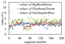
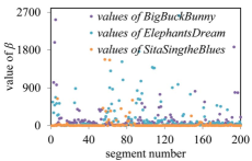
Figure 4: Quality model parameters (a) $\alpha_{1}$, $\alpha_{2}$, $\alpha_{3}$ and (b) $\beta_{1}$, $\beta_{2}$, $\beta_{3}$ of the video datasets in the simulation.

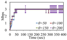
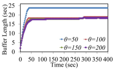
Figure 5: Results of case 1, in which two identical users compete the server export bandwidth of 6Mbps, and request the BigBuckBunny video sequence with learning rate $\theta=50$, 100, 150, and 200. Here, $\mu=0.003$, $\nu=0.0041$, $\alpha=2.15$, $\beta=0.0827$, $r^{\ast}=3$ Mbps, and $B_{W}=6$ Mbps and the inequality relation of (29) is tenable. (a) dynamic behavior of requested bitrates, (b) actual buffer lengths of the two users. Note that the states of the two users are identical.

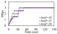
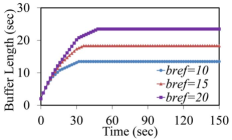
Figure 6: Results of case 1, in which two identical users compete the server export bandwidth of 6Mbps, and request the BigBuckBunny video sequence with learning rate $\theta=100$. Here, $\mu=0.003$, $\nu=0.0041$, $\alpha=2.15$, $\beta=0.0827$, $r^{\ast}=3$ Mbps, and $B_{W}=6$ Mbps and the inequality relation of (29) is tenable. (a) dynamic behavior of requested bitrates, (b) actual buffer lengths of the two users with the reference buffer lengths of 10s, 15s, and 20s respectively. Note that the states of the two users are identical.

Table II: Comparisons of Average Quality and Average Number of Switches of the Proposed Method with Different Learning Rates under Case 1

Learning Rate $\theta$	50	100	150	200
Average Bitrate (Mbps)	2.822	2.858	2.862	2.862
Average PSNR (dB)	44.602	44.700	44.683	44.654
Average SSIM	0.996	0.997	0.997	0.997
Average Number of Switches	12	11	17	67

4.2 Results of Case 1

In this case, two users compete the limited server export bandwidth of size 6Mbps. The reference buffer length is set as 15s. Fig. 5 shows the requested bitrates and buffer lengths of the two users by the proposed method with different learning rates. We can observe that the Nash Equilibrium is achieved at $r^{\ast}=3$ Mbps, and the actual buffer length converges to 15-20s except for the case where the learning rate equals 50. When the learning rate increases (e.g., $\theta=200$), the requested bitrate varies severely; however, the reference buffer is achieved more accurately as shown in Fig. 5. TABLE II compares the average requested bitrate and bitrate switching frequency of the proposed method with different learning rates ($\theta$). We can observe that the average requested bitrates are similar, while the minimum bitrate switching frequency is achieved when $\theta=100$.

Taking the learning rate of $\theta=100$ as an example, Fig. 6 shows that the Nash Equilibrium is achieved in a slower pace with the reference buffer increasing. Specifically, the converged buffer lengths are 13.32s, 17.93s, and 22.68s when the reference buffer lengths are set as 10s, 15s, and 20s, respectively. The reason is that the buffer needs more time to accumulate.

4.3 Results of Case 2

We verify the proposed method with a varied server export bandwidth that is realized via three types of variations [52], i.e., persistent variation, staged variation, and short-term variation, as shown in Fig. 7. The persistent and staged bandwidth variations (both increment and decrement) that last for tens of seconds appear frequently in practice when the cross traffic in the path’s bottleneck varies significantly due to arriving or departing traffic of some users. A good rate adaptation method should adapt to such variations by decreasing or increasing the requested bitrate. The short-term variation that lasts for only a few seconds is usually caused by burst change of channel states. For such short-term variations, the user should be able to keep requested bitrate stable to avoid unnecessary bitrate variations.

Fig. 8 shows the requested bitrates and buffer lengths of two users by the proposed method when the server export bandwidth exhibits persistent variation. We can observe that the requested bitrate increases to the Nash Equilibrium rapidly, and the reference buffer is also reached before $t=50$s. When the server export bandwidth varies to 9 Mbps at the time of 100s, the requested bitrate with $\theta=100$ quickly increases to 4.5 Mbps, while the requested bitrate with $\theta=50$ firstly increases to 5 Mbps, which consumes about 5s playout buffer before dropping to 4.5 Mbps. When the available bandwidth decreases back to 6 Mbps at the time of 200s, the requested bitrate with $\theta=100$ drops to 3 Mbps directly, while the requested bitrate with $\theta=50$ firstly drops to 3.5 Mbps. When the available bandwidth increases back to 9 Mbps at the time of 300s, the requested bitrate with $\theta=50$ steps to 4.5 Mbps, while the requested bitrate with $\theta=100$ increases to 4.5 Mbps directly. We can conclude that a larger learning rate can follow the bandwidth variation accurately and keep the buffer lengths more stable, while the requested bitrate is more stable for a smaller learning rate.

Fig. 9 shows the requested bitrates and buffer lengths of two users by the proposed method when the server export bandwidth exhibits staged variation. Similarly, we can also observe that the requested bitrate with a smaller learning rate (e.g., $\theta=50$) is more stable and the bitrate fluctuations are smaller at the time of bandwidth changing (i.e., at 100s, 180s, 260s, and 340s). However, the buffer length is further away from the reference buffer length than the learning rate of $\theta=100$. Nevertheless, the Nash Equilibrium can be achieved under both cases.

For the case of short-term server export bandwidth variation, the requested bitrate with a smaller learning rate ($\theta=50$) is more stable, as shown in Fig. 10. The requested bitrate with a smaller learning rate can avoid abrupt short-term changing by accumulating/consuming buffered video segments when encountering a small amplitude bandwidth variation, e.g., at the time of 100s and 260s, as shown in Fig. 10. But, the difference between the actual buffer length and the reference buffer length of $\theta=50$ is larger than that of the larger learning rate, i.e., $\theta=100$, as shown in Fig. 10.

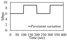
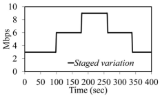
Figure 7: Three kinds of server bandwidth variations, (a) persistent variation, (b) staged variation, (c) short-term variation.

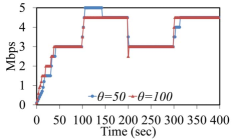
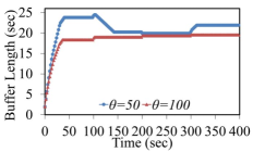
Figure 8: Results of case 2, in which two identical users compete the server export bandwidth with persistent variation, and request the BigBuckBunny video sequence with learning rate $\theta=50$ and 100 respectively. Here, $\mu=0.003$, $\nu=0.0041$. (a) dynamic behavior of requested bitrates, (b) actual buffer lengths of the two users with the reference buffer length of 15s. The initial server export bandwidth is 6Mbps. Note that the states of the two users are identical.

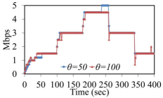
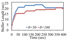
Figure 9: Results of case 2, in which two identical users compete the server export bandwidth with staged variation, and request the BigBuckBunny video sequence with learning rate $\theta=50$ and 100 respectively. Here, $\mu=0.003$, $\nu=0.0041$. (a) dynamic behavior of requested bitrates, (b) actual buffer lengths of the two users with the reference buffer length of 15s. The initial server export bandwidth is 6Mbps. Note that the states of the two users are identical.

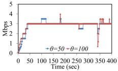
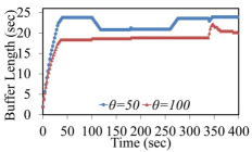
Figure 10: Results of case 2, in which two identical users compete the server export bandwidth with short-term variation, and request the BigBuckBunny video sequence with learning rate $\theta=50$ and 100 respectively. Here, $\mu=0.003$, $\nu=0.0041$. (a) dynamic behavior of requested bitrates, (b) actual buffer lengths of the two users with the reference buffer length of 15s. The initial server export bandwidth is 6Mbps. Note that the states of the two users are identical.

4.4 Results of Case 3

This subsection presents the performance of the proposed algorithm under Case 3, in which three users request three different videos (i.e., BigBuckBunny for User1, ElephantsDream for User2, and SitaSingstheBlues for User3) with a varied server export bandwidth. Note that the channel throughput of each user is limited up to 1.5 Mbps, which is unknown to the users, and the server export bandwidth is set as 6 Mbps. The reference buffer length is set as 15s. From Fig. 11, we can observe that the Nash Equilibrium is achieved with $r_{1}^{*}=1.5$ Mbps, $r_{2}^{*}=1.5$ Mbps, and $r_{3}^{*}=1.5$ Mbps, for different server export bandwidth variation scenarios, and no playback interruption occurs.

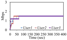
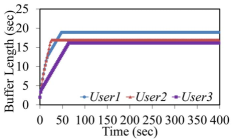
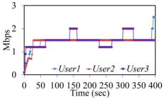
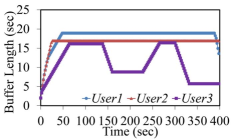
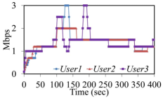
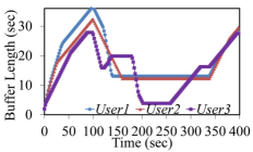
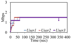
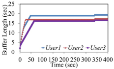
Figure 11: Results of case 3, in which three users (with fixed and limited throughputs of 1.5 Mbps) compete the server export bandwidth (6 Mbps), and request BigBuckBunny, ElephantsDream, and SitaSingstheBlues, respectively, with learning rate $\theta=50$. Here, $\mu=0.003$, $\nu=0.0041$. (a), (c), (e), and (g) show the requested bitrates for fixed, persistent variation, staged variation, and short-term variation of server export bandwidth. (b), (d), (f), and (h) show the corresponding buffer length of each user.

4.5 Results of Case 4

In addition, we also compare the proposed method (denoted by Proposed) with other methods (i.e., BF, QF, and QBA) with random user channel throughput limitations that are also unknown for each user.

Fig. 12 compares the requested bitrate and the buffer length of each user when the server export bandwidth is fixed to 6 Mbps. We can observe that the BF method switches the video bitrate frequently (see Fig. 12) in order to ensure the actual buffer length is close to the reference buffer length (see Fig. 12). As shown in Figs. 12 and (d), the QF method first accumulates a certain buffer length, and then struggles to request the highest bitrates, resulting in frequent re-buffering and bitrate switching. For the QBA method, its requested bitrates are more stable than those of BF and QF methods, but the buffer lengths of the three users are not fair, i.e., the buffer length of User3 is much smaller than that of User1 and User2, as shown in Figs. 12 and (f). The reason is that the QBA method does not take the fairness of users into consideration too much. From Figs. 12 and (h), it can be observed that the requested video bitrates by the Proposed method are stable for all of the three users, and their buffer lengths of the three users vary around the reference buffer length (set as 15s). Besides, there is no re-buffering (playback interruption) for the Proposed method.

Similar to Fig. 12, the corresponding comparison results of the four methods with respect to the other three types of bandwidth variations, i.e., persistent variation, staged variation, and short-term variation, are given in Figs. 13, 14, and 15, respectively. Similar conclusions can be drawn, which consistently demonstrates the superiority of the proposed algorithm.

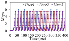
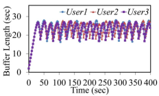
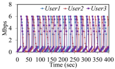
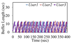
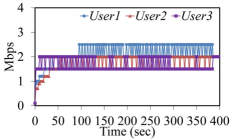
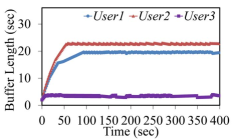
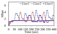
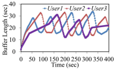
Figure 12: Results of case 4, in which three users (with random and limited throughputs) compete the server export bandwidth (fixed 6 Mbps), and request BigBuckBunny, ElephantsDream, and SitaSingstheBlues, respectively, with learning rate $\theta=50$. Here, $\mu=0.003$, $\nu=0.0041$. (a), (c), (e), and (g) show the requested bitrates of BF, QF, QBA, and the Proposed methods; while (b), (d), (f), and (h) show the corresponding buffer length of each user.

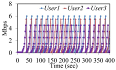
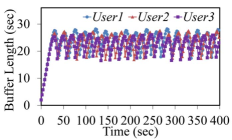
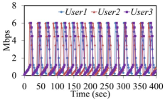
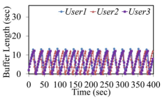
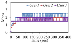
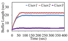
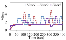
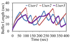
Figure 13: Results of case 4, in which three users (with random and limited throughputs) compete the server export bandwidth (persistent variation), and request BigBuckBunny, ElephantsDream, and SitaSingstheBlues, respectively, with learning rate $\theta=50$. Here, $\mu=0.003$, $\nu=0.0041$. (a), (c), (e), and (g) show the requested bitrates of BF, QF, QBA, and the Proposed methods; while (b), (d), (f), and (h) show the corresponding buffer length of each user.

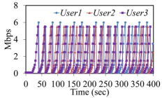
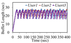
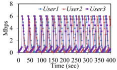
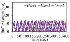
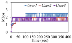
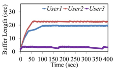
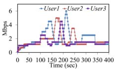
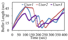
Figure 14: Results of case 4, in which three users (with random and limited throughputs) compete the server export bandwidth (staged variation), and request BigBuckBunny, ElephantsDream, and SitaSingstheBlues, respectively, with learning rate $\theta=50$. Here, $\mu=0.003$, $\nu=0.0041$. (a), (c), (e), and (g) show the requested bitrates of BF, QF, QBA, and the Proposed methods; while (b), (d), (f), and (h) show the corresponding buffer length of each user.

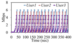
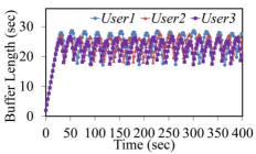
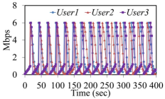
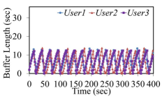
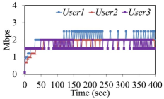
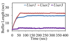
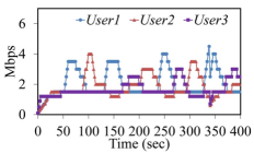
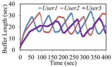
Figure 15: Results of case 4, in which three users (with random and limited throughputs) compete the server export bandwidth (short-term variation), and request BigBuckBunny, ElephantsDream, and SitaSingstheBlues, respectively, with learning rate $\theta=50$. Here, $\mu=0.003$, $\nu=0.0041$. (a), (c), (e), and (g) show the requested bitrates of BF, QF, QBA, and the Proposed methods; while (b), (d), (f), and (h) show the corresponding buffer length of each user.

Table III: Detailed Comparisons of the Four Methods under Case 4 (The best results are bolded).

Detailed numerical comparisons of the four methods are given in TABLE III, from which we can observe that the average received bitrate of the QF method is largest, but the bitrate fluctuations (see the standard deviation, average number of switches and average switching amplitude of received bitrates) are also the maximum, and there exist playback interruptions, while the bitrate fluctuation of the BF method is a little small but still large. It can also be observed that the average video quality (by observing the average SSIMs) of the QF and BF methods is obviously lower than that of the QBA and the Proposed methods, and the quality variations (by observing the standard deviation of SSIM values of received video segments) of the QF and the BF methods are larger than those of the QBA and the Proposed methods. Moreover, although the average bitrates and SSIM values of the Proposed method are similar to those of the QBA method, it is obvious that the amplitudes of bitrate switching and the numbers of switches of Proposed method are smaller, which means that the performance of the Proposed method is the best.

Table IV: Comparisons of the Four Methods under Case 4 in terms of the QoE metric in [53] (The best results are bolded)

Table V: Comparisons of the Four Methods under Case 4 in terms of the QoE metric in [54] (The best results are bolded)

Last, we evaluate the performance of the four algorithms, i.e., BF, QF, QBA, and Proposed, by comparing their produced QoE values that are measured via two extensively used QoE models [53][54]:

$$QoE_{1}= \sum^{M}_{k=1}r[k]-\xi\sum^{M-1}_{k=1}|r[k+1]-r[k]|$$ (34)

$$-\psi\sum^{M}_{k=1}\max\{0,T_{down}[k]-b[k]\},$$

$$QoE_{2}= \sum^{M}_{k=1}q[k]-\varphi\sum^{M-1}_{k=1}|q[k+1]-q[k]|$$ (35)

$$-\sigma\sum^{M-1}_{k=1}\left(\max\left(0,b_{ref}-b[k+1]\right)\right)^{2}$$

$$-\eta\sum^{M}_{k=1}\max\{0,T_{down}[k]-b[k]\},$$

where $\xi=1$, $\psi=6$, $\varphi=2$, $\sigma=0.001$ and $\eta=2$ are model parameters that are empirically defined in [53] and [54], M is the number of received segments, $r[k]$ is the bitrate of the $k^{th}$ requested video segment, $q[k]$ is the corresponding SSIM value, $T_{down}[k]$ is the download time of the $k^{th}$ segment, and $b[k]$ is the buffer length at the end time of the $k^{th}$ segment and $b_{ref}=15$s. Note that we set $\eta$ to 2 instead of 50 in [54] to ensure that the QoE values are positive. From TABLE IV and V, it can be observed that, compared with the other three methods, the proposed algorithm always produces the highest average QoE with respect to different types of bandwidth variations. Besides, the proposed method provides optimal QoE for most users, i.e., at least 2 out of 3 users.

5 Experimental Result for Realistically Modeled Networking Scenarios

We also established realistically modeled wireless and wired networking scenarios, in which 6 users requested different videos from a single server. In the wireless network, they were connected by a movable router (2.4GHz, automatic frequency channel bandwidth, 802.11b/g/n mixed wireless mode, 1480 Byte maximum transmission unit configuration); yet in the wired network, the users connected to the server via the campus network of Shandong University which includes many switches and routers. To ensure a large server export bandwidth (which can be constrained to 6Mbps by DummyNet), the experiments were conducted at night. The initial buffer of each user was set as 20s in the experiments in order to calculate the initial playout delay. The performance of the proposed algorithm was verified under 2 cases:

Case 1, 6 users requested different video contents all the time;

Case 2, 6 users requested different video contents at the beginning, and then some users leaved or joined the network.

5.1 Results of Case 1

The results of the wireless and wired networks are given in Figs. 16 and 17, respectively. We can observe that the fluctuations of the requested bitrates and buffer lengths are larger than those of the simulated networking scenario because of the complexity of the realistic networking environment. From TABLE VI, we can observe that the average initial playout delays of the QF and the BF methods are similar, i.e., 3.61s and 2.70s, for the wireless networking environment and 0.88s and 1.47s for the wired networking environment. Similar to the results of the simulation, the average received bitrates of the Proposed method are not the largest but are comparable with the other methods. More importantly, we can see that there is no playback interruption under both the wireless and wired networking environment for the proposed algorithm, which is also demonstrated in Figs. 16 and 17. As shown in TABLE VI, although there is also no playback interruption for the BF method, the received bitrate fluctuations (average standard deviation) of all the 6 users are much larger than the Proposed method. From Figs. 16 and 17, we can see that the requested bitrates of the Proposed method fluctuate around 1Mbps (the total server export bandwidth is set as 6Mbps). Moreover, the average buffer length of the Proposed method is the largest, which means that the performance of the Proposed method can cope with network variations better.

Because DASH achieves lossless transmission to improve the QoE of users at the cost of transmitting additional signaling information of TCP for HTTP sessions between the server and user, the overhead problem is common and inevitable in DASH. The signaling overhead is essentially determined by the number of HTTP sessions. Therefore, we also investigated the signaling overhead of the information exchanges between servers and users in the proposed algorithm, as shown in TABLE VII. We have to clarify that the reported signaling overhead in our manuscript is calculated as the time ratio of the download time of overhead information to that of the video segments. It can be observed that the average proportion of the signaling overhead induced by the information exchanges is about 30% of the whole download time. It is worth pointing out that by using additional HTTP sessions, the performance of a DASH system can be improved.

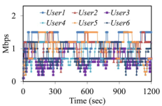
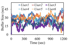
Figure 16: Experimental Results of realistically modeled wireless network, in which 6 users compete the server export bandwidth (6 Mbps) with $\theta=40$, $\mu=0.003$, and $\nu=0.0041$, (a) dynamic behavior of requested bitrates, (b) the actual buffer lengths of the 6 users with the reference buffer length of 20s.

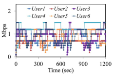
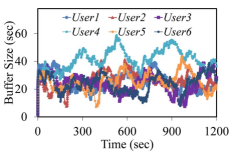
Figure 17: Experimental Results of realistically modeled wired network, in which 6 users compete the server export bandwidth (6 Mbps) with $\theta=30$, $\mu=0.003$, and $\nu=0.0041$, (a) dynamic behavior of requested bitrates, (b) the actual buffer lengths of the 6 users with the reference buffer length of 20s.

Table VI: Performance Comparisons of Different Methods

Table VII: The Proportion of Signaling Overhead Introduced by the Information Exchanges between Server and Users

5.2 Results of Case 2

We verified the performance of the proposed algorithm when users’ requests dynamically come and leave at different times (i.e., User5 leaves at about 600s and joins at 900s, User6 leaves at about 300s and joins at 1200s). Experimental results are shown in Figs. 18 (wireless) and 19 (wired). From Figs. 18 and 19, we can observe that when User 5 and 6 leave, the requested bitrates of the remaining users increase to 1.5Mbps gradually, while the requested video bitrates of all the users gradually converge to 1Mbps when User 5 and 6 join again. Accordingly, the effectiveness of the proposed algorithm is demonstrated for the realistic network scenario with dynamic user leaving or joining.

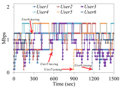
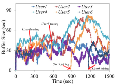
Figure 18: Experimental Results of realistically modeled wireless network, in which users’ requests come and leave at different time (User5 leaving at about 600s and joining at 900s, User6 leaving at about 300s and joining at 1200s), with $\theta=40$, $\mu=0.003$, and $\nu=0.0041$, and the server export bandwidth is 6Mbps, (a) dynamic behavior of requested bitrates, (b) the actual buffer lengths of the 6 users with the reference buffer length of 20s.

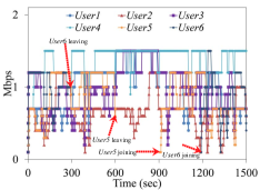
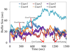
Figure 19: Experimental Results of realistically modeled wired network, in which users’ requests come and leave at different time (User5 leaving at about 600s and joining at 900s, User6 leaving at about 300s and joining at 1200s), with $\theta=40$, $\mu=0.003$, and $\nu=0.0041$, and the server export bandwidth is 6Mbps, (a) dynamic behavior of requested bitrates, (b) the actual buffer lengths of the 6 users with the reference buffer length of 20s.

6 Conclusion And Discussion

In this paper, we have presented a novel non-cooperative game theory based algorithm to address the rate adaptation issue posed in a DASH system with single-server and multi-users. The proposed algorithm can not only guarantee user fairness but also improve user QoE. Moreover, no proxy is required with our algorithm. We have formulated the rate adaptation problem as a non-cooperative game by building a novel user QoE model that considers the received video quality, reference buffer length, and accumulated buffer lengths of users. We have theoretically proven the existence of the Nash Equilibrium of our specific game, which can be found by our distributed iterative algorithm with stability analysis. Simulation and experimental results show that the quality and bitrates of received videos by the proposed algorithm are more stable than the state-of-the-art methods, while the actual buffer length of each user moves around the reference buffer all the time. Besides, there is no playback interruption for the proposed algorithm.

Although the proposed rate adaptation algorithm can achieve impressive performance compared with existing algorithm, we believe it can be further improved by addressing the following limitations:

(1) Restriction on the QoE model. In order to guarantee the existence of the Nash Equilibrium, the QoE model must be designed as a continuous and quasi-concave function with respect to the bitrates of all the users.

(2) Stability analysis of the scenarios with multi-users or users joining and leaving dynamically. In the proposed method, we used a distributed iterative algorithm to obtain the Nash Equilibrium. However, the stability of the distributed iterative algorithm is analyzed in detail for the scenario with only 2 users. When there are more than 2 users, the stability analysis will be very complex, and we only provide a sketch. Besides, for the scenario with new users joining/leaving dynamically, the stability analysis of the proposed method is not analyzed well.

(3) Additional HTTP sessions. For the proposed method, additional HTTP sessions between users and servers are needed to achieve the Nash Equilibrium, which will introduce additional signaling overhead. Such signaling overhead may result in latency. Although this is a common drawback of DASH, it is also highly desirable to develop new algorithms to reduce the additional HTTP sessions as much as possible.

References

- [1] C. Begen, T. Akgul, M. Baugher, “Watching Video over the Web, Part I: Streaming Protocols,” IEEE Int. Comput., vol. 15, no. 2, pp. 54-63, Mar. 2011.
- [2] A. C. Begen, T. Akgul, M. Baugher, “Applications, Standardization, and Open Issues,” IEEE Int. Comput., vol. 15, no. 3, pp. 59-63, Apr. 2011.
- [3] ISO/IEC IS 23009-1: “Information Technology - Dynamic Adaptive Streaming over HTTP (DASH) - Part 1: Media Presentation Description and Segment Formats,” 2012.
- [4] T. Stockhammer, “Dynamic Adaptive Streaming over HTTP - Standards and Design Principles,” in Proc. ACM Multimedia Systems Conference, California, Feb. 2011, pp.133-144.
- [5] D. K. Krishnappa, D. Bhat and M. Zink, “DASHing YouTube: An Analysis of Using DASH in YouTube Video Service,” in Proc. IEEE Conf. Local Computer Networks, Sydney, NSW, 2013, pp. 407-415.
- [6] C. Wang, A. Rizk, M. Zink, “SQUAD: A Spectrum-Based Quality Adaptation for Dynamic Adaptive Streaming over HTTP,” in Proc. International Conference on Multimedia Systems, Klagenfurt, Austria, May. 2016.
- [7] J. Nash, “Non-cooperative games,” Annals of Mathematics, pp. 286-295, vol. 54, 1951.
- [8] J. Luo, I. Ahmad and Y. Sun, “Controlling the Bit Rate of Multi-Object Videos with Noncooperative Game Theory,” IEEE Trans. Multimedia, vol. 12, no. 2, pp. 97-107, Feb. 2010.
- [9] P. Goudarzi, “A Non-cooperative Quality Optimization Game for Scalable Video Delivery over MANETs,” Wireless Networks, vol. 19, no. 5, pp. 755-770, 2013.
- [10] A. Cournot, Researches into the Mathematical Principles of the Theory of Wealth, NT Bacon Trans., 1927.
- [11] T. C. Thang, Q. D. Ho, J. W. Kang and A. T. Pham, “Adaptive Streaming of Audiovisual Content Using MPEG DASH,” IEEE Trans. Consumer Electron., vol. 58, no. 1, pp. 78-85, Feb. 2012.
- [12] L. R. Romero, “A Dynamic Adaptive HTTP Streaming Video Service for Google Android,” M.S. Thesis, Royal Institute of Technology (KTH), Stockholm, Oct. 2011.
- [13] T. C. Thang, H. T. Le, H. X. Nguyen, A. T. Pham, J. W. Kang and Y. M. Ro, “Adaptive Video Streaming over HTTP with Dynamic Resource Estimation,” Communications and Networks, vol. 15, no. 6, pp. 635-644, Dec. 2013.
- [14] C. Liu, I. Bouazizi, M. M. Hannuksela and M. Gabbouj, “Rate Adaptation for Dynamic Adaptive Streaming over HTTP in Content Distribution Network,” Signal Process. Image Commun., vol. 27, no. 4, pp. 288-311, 2012.
- [15] T.-Y. Huang, N. Handigol, B. Heller, N. McKeown, and R. Johari, “Confused, timid, and unstable: Picking a video streaming rate is hard,” in Proc. ACM Conf. Internet Meas. Conf., Nov. 2012, pp. 225-238.
- [16] H. Mao, R. Netravali, and M. Alizadeh, “Neural adaptive video streaming with Pensieve,” in Proc. Conference of the ACM Special Interest Group on Data Communication (SIGCOMM’17), pp. 197-210, Los Angeles, CA, USA, Aug. 21.
- [17] M. Li, C.-Y. Lee, “A Cost-Effective and Real-Time QoE Evaluation Method for Multimedia Streaming Services,” Telecommunication Systems, vol. 59, no. 3, pp. 317-327, Jul. 2015.
- [18] Z. Duanmu, K. Zeng, K. Ma, A. Rehman, and Z. Wang, “A quality-of-experience index for streaming video,” IEEE Journal of Selected Topics in Signal Processing, vol. 11, no. 1, pp. 154-166, Feb. 2017.
- [19] W. Zhang, Y. Wen, Z. Chen and A. Khisti, “QoE-Driven Cache Management for HTTP Adaptive Bit Rate Streaming Over Wireless Networks,” IEEE Trans. Multimedia, vol. 15, no. 6, pp. 1431-1445, Oct. 2013.
- [20] A. Parandeh Gheibi, M. Medard, A. Ozdaglar, and S. Shakkottai, “Avoiding Interruptions - A QoE Reliability Function for Streaming Media Applications,” IEEE J. Sel. Area Commun., vol. 29, no. 5, pp. 1064-1074, May. 2011.
- [21] Y. Xu, Y. Zhou and D. M. Chiu, “Analytical QoE Models for Bit-Rate Switching in Dynamic Adaptive Streaming Systems,” IEEE Trans. Mobile Computing, vol. 13, no. 12, pp. 2734-2748, Dec. 2014.
- [22] D. Zegarra Rodríguez, R. Lopes Rosa, E. Costa Alfaia, J. Issy Abraho and G. Bressan, “Video Quality Metric for Streaming Service Using DASH Standard,” IEEE Trans. Broadcast., vol. 62, no. 3, pp. 628-639, Sept. 2016.
- [23] C. Zhou, C. W. Lin and Z. Guo, “mDASH: A Markov Decision-Based Rate Adaptation Approach for Dynamic HTTP Streaming,” IEEE Trans. Multimedia, vol. 18, no. 4, pp. 738-751, Apr. 2016.
- [24] V. Martín, J. Cabrera and N. García, “Design, Optimization and Evaluation of A Q-Learning HTTP Adaptive Streaming Client,” IEEE Trans. Consumer Electron., vol. 62, no. 4, pp. 380-388, Nov. 2016.
- [25] A. Bokani, M. Hassan, S. Kanhere and X. Zhu, “Optimizing HTTP-Based Adaptive Streaming in Vehicular Environment Using Markov Decision Process,” IEEE Trans. Multimedia, vol. 17, no. 12, pp. 2297-2309, Dec. 2015.
- [26] J. Jiang, V. Sekar and H. Zhang, “Improving Fairness, Efficiency, and Stability in HTTP-Based Adaptive Video Streaming With Festive,” IEEE/ACM Trans. Networking, vol. 22, no. 1, pp. 326-340, Feb. 2014.
- [27] Z. Li, X. Zhu, J. Gahm, R. Pan, H. Hu, A. C. Begen and D. Oran, “Probe and Adapt: Rate Adaptation for HTTP Video Streaming at Scale,” IEEE J. Select. Areas Commun., vol. 32, no. 4, pp. 719-733, April 2014.
- [28] A. E. Essaili, D. Schroeder, E. Steinbach, D. Staehle and M. Shehada, “QoE-Based Traffic and Resource Management for Adaptive HTTP Video Delivery in LTE,” IEEE Trans. Circuits Syst. Video Technol., vol. 25, no. 6, pp. 988-1001, Jun. 2015.
- [29] Z. Su, Q. Xu, M. Fei and M. Dong, “Game Theoretic Resource Allocation in Media Cloud with Mobile Social Users,” IEEE Trans. Multimedia, vol. 18, no. 8, pp. 1650-1660, Aug. 2016.
- [30] S. Wang, A. Rehman, Z. Wang, S. Ma and W. Gao, “SSIM-Motivated Rate-Distortion Optimization for Video Coding,” IEEE Trans. Circuits Syst. Video Technol., vol. 22, no. 4, pp. 516-529, Apr. 2012.
- [31] G. Tian and Y. Liu, “Towards Agile and Smooth Video Adaptation in HTTP Adaptive Streaming,” IEEE/ACM Trans. Networking, vol. 24, no. 4, pp. 2386-2399, Aug. 2016.
- [32] P. D. Straffin, “Game Theory and Strategy,” The Mathematical Association of America, Washington, DC, 1993.
- [33] S. Boyd and L. Vandenberghe, Convex Optimization, 6th ed. Cambridge, U.K.: Cambridge Univ. Press, 2008, pp. 67-71.
- [34] S. Boyd, X. Lin and A. Mutapcic, Subgradient Methods, Stanford University, Oct. 2003.
- [35] P. Tsiaflakis, I. Necoara, J. A. K. Suykens and M. Moonen, “Improved Dual Decomposition Based Optimization for DSL Dynamic Spectrum Management,” IEEE Trans. Signal Processing, vol. 58, no. 4, pp. 2230-2245, Apr. 2010.
- [36] Z. Zhou, M. Dong, K. Ota, J. Wu and T. Sato, “Energy Efficiency and Spectral Efficiency Tradeoff in Device-to-Device (D2D) Communications,” IEEE Wirel. Commun. Letters, vol. 3, no. 5, pp. 485-488, Oct. 2014.
- [37] D. Niyato and E. Hossain, “Competitive Spectrum Sharing in Cognitive Radio Networks: A Dynamic Game Approach,” IEEE Trans. Wireless Commun., vol. 7, no. 7, pp. 2651-2660, Jul. 2008.
- [38] M. Sonis, “Once More on Henon Map: Analysis of Bifurcations” Chaos, Solitons and Fractals, vol. 7, no. 12, pp. 2215-2234, 1996.
- [39] H. N. Agiza, G.-I. Bischi, and M. Kopel, “Multistability in a Dynamic Cournot Game with Three Oligopolists,” Mathematics and Computers in Simulation, vol. 51, pp. 63-90, 1999.
- [40] E. Ahmed and H. N. Agiza, “Dynamics of a Cournot Game with n Competitors,” Chaos, Solitons & Fractals, vol. 9, pp. 1513-1517.
- [41] C. Mueller, S. Lederer, J. Poecher and C. Timmerer, “Demo paper: Libdash - An Open Source Software Library for the MPEG-DASH Standard,” in Proc. IEEE Int. Conf. Multimedia and Expo Workshops (ICMEW), San Jose, CA, 2013, pp. 1-2.
- [42] C. Alberti, D. Renzi, C. Timmerer, C. Mueller, S. Lederer, S. Battista and M. Mattavelli, “Automated QoE Evaluation of Dynamic Adaptive Streaming over HTTP,” in Proc. the 5th International Workshop on Quality of Multimedia Experience, IEEE, Los Alamitos, CA, USA, 2013, pp. 58-63.
- [43] Apache HTTP Server Project, http://httpd.apache.org/, (last access: Jan. 2017).
- [44] L. Rizzo, “Dummynet: A Simple Approach to The Evaluation of Network Protocols,” ACM Computer Communication Review, vol. 27, no. 1, pp. 31-41, Jan. 1997.
- [45] Big Buck Bunny Movie, http://www.bigbuckbunny.org/, (last access: Jan. 2017).
- [46] C. Mueller, S. Lederer and C. Timmerer, “An Evaluation of Dynamic Adaptive Streaming over HTTP in Vehicular Environments,” in Proc. the Fourth Annual ACM SIGMM Workshop on Mobile Video, ACM, New York, NY, USA, 2012, pp. 37-42.
- [47] Elephants Dream Movie, http://www.elephantsdream.org/, (last access: Jan. 2017).
- [48] Sita Sing the Blues Movie, http://www.sitasingstheblues.com/, (last access: Jan. 2017).
- [49] S. Lederer, C. Müller and C. Timmerer, “Dynamic Adaptive Streaming over HTTP Dataset,” in Proc. the ACM Multimedia Systems Conference 2012, Chapel Hill, North Carolina, 2012, Feb. 22-24.
- [50] S. Lederer, C. Mueller, C. Timmerer, C. Concolato, J. L. Feuvre and K. Fliegel, “Distributed DASH Dataset,” in Proc. the 4th ACM Multimedia Systems Conference, ACM, New York, NY, USA, 2013, pp. 131-135.
- [51] M. Drxler and H. Karl, “Cross-layer Scheduling for Multi-Quality Video Streaming in Cellular Wireless Networks,” in Proc. Int. Wirel. Commun. and Mobile Comput. (IWCMC), Sardinia, 2013, pp. 1181-1186.
- [52] S. Akhshabi, S. Narayanaswamy, A. C. Begen and C. Dovrolis, “An Experimental Evaluation of Rate-Adaptive Video Players over HTTP,” Signal Processing Image Communication, vol. 27, no. 4, pp. 271-287, 2012.
- [53] X. Yin, V. Sekar and B. Sinopoli, “Toward a Principled Framework to Design Dynamic Adaptive Streaming Algorithms over HTTP.” in Proc. Workshop on Hot Topics in Networks, ACM, Sept. 2014.
- [54] F. Chiariotti, S. D’Aronco, L. Toni and P. Frossard, “Online Learning Adaptation Strategy for DASH Clients,” in Proc. Multimedia Systems, ACM, Aug. 2016.