Stochastic Dynamic Cutting Plane for multistage stochastic convex programs
Abstract.
We introduce StoDCuP (Stochastic Dynamic Cutting Plane), an extension of the Stochastic Dual Dynamic Programming (SDDP) algorithm to solve multistage stochastic convex optimization problems. At each iteration, the algorithm builds lower bounding affine functions not only for the cost-to-go functions, as SDDP does, but also for some or all nonlinear cost and constraint functions. We show the almost sure convergence of StoDCuP. We also introduce an inexact variant of StoDCuP where all subproblems are solved approximately (with bounded errors) and show the almost sure convergence of this variant for vanishing errors. Finally, numerical experiments are presented on nondifferentiable multistage stochastic programs where Inexact StoDCuP computes a good approximate policy quicker than StoDCuP while SDDP and the previous inexact variant of SDDP combined with Mosek library to solve subproblems were not able to solve the differentiable reformulation of the problem.
|
|
Keywords: Stochastic programming, Inexact cuts for value functions, SDDP, Inexact SDDP.
AMS subject classifications: 90C15, 90C90.
1. Introduction
Risk-neutral multistage stochastic programs (MSPs) aim at minimizing the expected value of the total cost over a given optimization period of stages while satisfying almost surely for every stage some constraints depending on an underlying stochastic process. These optimization problems are useful for many real-life applications but are challenging to solve, see for instance [33] and references therein for a thorough discussion on MSPs. Popular solution methods for MSPs are based on decomposition techniques such as Approximate Dynamic Programming [27], Lagrangian relaxation, or Stochastic Dual Dynamic Programming (SDDP) [23]. SDDP is a sampling-based extension of [3], itself a multistage extension of the L-shaped method [35]. The SDDP method builds linearizations of the convex cost-to-go functions at trial points computed on scenarios of the underlying stochastic process generated randomly along iterations. The use of such cutting plane models for the objective function in the context of deterministic convex optimization dates back to Kelley’s cutting plane method [16] and has later been extended in many variants such as subgradient [17], bundle [18, 20], and level [21] variants. Kelley’s algorithm was also generalized by Benders to solve [2] mixed-variables programming problems. Recently, several enhancements of SDDP have been proposed, see for instance [32], [12], [24], [19] for risk-averse variants, [26], [5], [6] for convergence analysis, [34] for the application of SDDP to periodic stochastic programs, and [22], [8] to speed up the convergence of the method. In particular, in [8], Inexact SDDP was proposed, which incorporates inexact cuts in SDDP (for both linear and nonlinear programs). The idea of Inexact SDDP is to allow us to solve approximately some or all primal and dual subproblems in the forward and backward passes of SDDP. This extension and the study of Inexact SDDP was motivated by the following reasons:
-
(i)
solving to a very high accuracy nonlinear programs can take a significant amount of time or may even be impossible whereas linear programs (of similar sizes) can be solved exactly or to high accuracy quicker. Examples of convex but challenging to solve subproblems include semidefinite programs [36], quadratically constrained quadratic programs with degenerate quadratic forms (see the numerical experiments of Section 5), or some high dimensional nondifferentiable problems. For subproblems where it is difficult or impossible to get optimal solutions, if we are able to provide a feasible primal-dual solution, we should be able to derive an extension of SDDP, i.e., cuts for the cost-to-go functions, from approximate subproblem primal-dual solutions. Therefore one has to study how to extend the SDDP algorithm to still derive valid cuts and a converging Inexact SDDP or an Inexact SDDP with controlled accuracy when only approximate primal and dual solutions are computed for nonlinear MSPs.
-
(ii)
As explained in [8], numerical experiments (see for instance [7, 10, 15]) indicate that very loose cuts are computed in the first iterations of SDDP and it may be useful to compute with less accuracy these cuts for the first iterations. Using this strategy, it was shown in [8] that for several instances of a portfolio problem, Inexact SDDP can converge (i.e., satisfy the stopping criterion) quicker than SDDP.
In this paper, we extend [8] in two ways:
-
•
a natural way of taking advantage of observation (i) above in the context of SDDP applied to nonlinear problems, consists in linearizing some or all nonlinear objective and constraint functions of the subproblems solved along the iterations of the method at the optimal solutions of these subproblems. When all nonlinear functions are linearized, all subproblems solved in the iterations of SDDP are linear programs which allows us to avoid having to solve difficult problems that cannot be solved with high accuracy. However, to the best of our knowledge, this variant of SDDP, that we term as StoDCuP (Stochastic Dynamic Cutting Plane) has not been proposed and studied so far in the literature (SDDP does build linearizations for the cost-to-go functions but not for some or all of the remaining nonlinear objective and constraint functions). In this context, the goal of this paper is to propose and study StoDCuP.
-
•
As far as (ii) is concerned, it is interesting to notice that it is easy to incorporate inexact cuts in StoDCuP (i.e., to derive an inexact variant of StoDCuP), control the quality of these cuts (see Lemma 4.1), and show the convergence of this method (see Theorem 4.3 below). This comes from the fact that we can easily compute a cut for the value function of a linear program (and in StoDCuP all subproblems solved are linear programs) from any feasible primal-dual solution since the corresponding dual objective is linear, see Proposition 2.1 in [8]. On the contrary, deriving valid (inexact) cuts from approximate primal-dual solutions of the subproblems solved in SDDP applied to nonlinear problems and showing the convergence of the corresponding variant of Inexact SDDP is technical and the computation of inexact cuts may require solving additional subproblems, see [8] for details. Moreover, Inexact SDDP from [8] applies to differentiable multistage convex stochastic programs while both StoDCuP and Inexact StoDCuP apply to more general differentiable or nondifferentiable multistage convex stochastic programs.
The outline of the paper is the following. To ease the presentation and analysis of StoDCuP, we start in Section 2 with its deterministic counterpart, called DCuP (Dynamic Cutting Plane) which solves convex Dynamic Programming equations linearizing cost-to-go, constraint, and objective functions. Starting with the deterministic case allows us to focus on the differences between traditional Dual Dynamic Programming and its convergence analysis with DCuP and its convergence analysis. In Section 3, we introduce forward StoDCuP and prove the almost sure convergence of the method. In Section 4, we present Inexact StoDCuP, an inexact variant of StoDCuP which builds inexact cuts on the basis of approximate primal-dual solutions of the subproblems solved along the iterations of the method. We also prove the almost sure convergence of Inexact StoDCuP for vanishing noises. Our convergence proofs of DCuP and StoDCuP are based on the convergence analysis of SDDP for nonlinear problems in [6] but additional technical results are needed due to the linearizations of cost and constraint functions, see Lemma 2.1-(c),(d), Lemma 2.2, Lemma 2.4-(b), Theorem 2.6-(i),(ii), Lemma 3.4-(c), Lemmas 3.7, 3.8, and Theorem 3.9. Finally, numerical experiments are presented in Section 5 on nondifferentiable multistage stochastic programs. Two variants of Inexact StoDCuP are presented: with and without cut selection strategies. In all instances tested, at least one inexact variant computes a good approximate policy quicker than StoDCuP while SDDP and the previous inexact variant of SDDP from [8] combined with Mosek library to solve subproblems were not able to solve a differentiable reformulation of the problem (recall that such reformulation is necessary to use the inexact variant of SDDP from [8] which applies to differentiable stochastic programs).
We will use the following notation:
-
•
For a real-valued convex function , we denote by an arbitrary lower bounding linearization of at , i.e., where is an arbitrary subgradient of at .
-
•
The domain of a point to set operator is given by Dom().
-
•
For vectors , is the usual scalar product between and .
-
•
For , .
-
•
The domain of a convex function is .
-
•
The relative interior ri of a set is the set .
-
•
The subdifferential of the convex function at is
-
•
The indicator function of the set is given by if and otherwise.
-
•
A function is proper if there is such that is finite.
-
•
e is a vector of ones whose dimension depends on the context.
2. The DCuP (Dynamic Cutting Plane) algorithm
2.1. Problem formulation and assumptions
Given , consider the optimization problem
| (2.1) |
where and are matrices of appropriate dimensions, and . In this problem, for each step , we have nonlinear and linear coupling constraints, and respectively, and set constraints . Without loss of generality, nonlinear noncoupling constraints can be dealt with by incorporating them into the constraint . For convenience, we use the short notation
| (2.2) |
and
| (2.3) |
With this notation, the dynamic programming equations corresponding to problem (2.1) are
| (2.4) |
for , and . The cost-to-go function represents the optimal total cost for time steps , starting from state at the beginning of step . Clearly, it follows from the above definition that
| (2.5) |
Setting , the following assumptions are made throughout this section.
Assumption (H1):
-
1)
For :
-
a)
is nonempty, convex, and compact;
-
b)
is a proper lower-semicontinuous convex function such that ;
-
c)
each of the components , of is a proper lower-semicontinuous convex function such that .
-
a)
-
2)
and for every .
The following simple lemma states a few consequences of the above assumptions.
Lemma 2.1.
The following statements hold:
-
(a)
for every , is a convex function such that
-
(b)
for every , is Lipschitz continuous on ;
-
(c)
for every , , and ,
-
(d)
for every , , the sets
are bounded.
Proof: (a) The proof is by backward induction on . The result clearly holds for since . Assume now that is a convex function such that for some . Then, condition 1) of Assumption (H1) implies that the function is convex. This conclusion together with the definition of and the discussion following Theorem 5.7 of [28] then imply that is a convex function. Moreover, conditions 1)b) and 2) of Assumption (H1) and relation (2.5) imply that there exists such that for every ,
The induction hypothesis, the latter observation, and relations (2.2) and (2.4), then imply that
for every . Since by (2.4),
we then conclude that , and hence that . We have thus proved that (a) holds.
b) This statement follows from statement a) and Theorem 10.4 of [28].
c-d) These two statements follow from conditions 1)a), 1)b) and 1)c) of Assumption (H1) together with Theorem 23.4 and 24.7 of [28].
2.2. Forward DCuP
Before formally describing the DCuP algorithm, we give some motivation for it. At iteration and stage , the algorithm uses the following approximation to the function defined in (2.4):
| (2.6) |
where
| (2.7) |
and , and are polyhedral functions minorizing and , respectively, i.e.,
| (2.8) |
For , we actually assume that , and hence that . Moreover, we also assume that , and hence .
Observe that for every , , and , relations (2.7) and (2.8) imply that
| (2.9) |
and
and hence that
| (2.10) |
At iteration , feasible points are computed recursively as follows: for , is set to be an optimal solution of subproblem (2.6) with with the convention that . These points in turn are used to compute new affine functions minorizing , and which are then added to the bundle of affine functions describing , , and to obtain new lower bounding approximations , and for and , respectively.
The precise description of DCuP algorithm is as follows.
DCuP (Dynamic Cutting Plane) with linearizations computed in a forward pass.
Step 0. Initialization.
For every , let affine functions and such that and ,
and a piecewise linear function
such that
be given. We write
as
,
set
, and .
Step 1. Forward pass. Set and . For , do:
- a)
-
b)
compute function values and subgradients of and , , at , and let and denote the corresponding linearizations;
-
c)
set
(2.12) (2.13) and define ;
-
d)
if , then compute and denote the corresponding linearization of as
moreover, set
(2.14)
Step 2. Set and go to Step 1.
We now make a few remarks about DCuP. First, Lemma 2.1(c) guarantees the existence of the subgradients, and hence the linearizations, of the functions and , , at any point , and hence that the functions and in Step 1 are well-defined. Second, in view of the definition of in Step a), we have that for every and . Third, Lemma 2.2(b) below and the previous remark guarantee the existence of the subgradient in Step d). Fourth, we dicuss in Subsection 2.3 ways of computing this subgradient.
In the remaining part of this subsection, we provide the convergence analysis of DCuP. The following result states some basic properties about the functions involved in DCuP.
Lemma 2.2.
The following statements hold:
-
(a)
for every and , we have
(2.15) (2.16) (2.17) (2.18) -
(b)
For every and , function is convex and ; as a consequence, for every .
Proof: (a) Relations (2.15) and (2.16) follow immediately from the initialization of DCuP described in step 0, the recursive definitions of and in (2.12) and (2.13), respectively, the definition of in (2.7), and the fact that
Next note that the inequalities in (2.18) follow immediately from the respective ones in (2.15), (2.16) and (2.17), together with relations (2.4) and (2.11). It then remains to show that the inequalities in (2.17) hold. Indeed, the inequality follows immediately from (2.14) with . We will now show that inequalities for every implies that for every , and hence that the second inequality in (2.17) follows from a simple inductive argument on . Indeed, first observe that the inequality implies that . Next observe that the construction of in Step d) of DCuP implies that , and hence that . It then follows from (2.14) and the inequality that . We have thus shown that for every implies that for every . Since the latter inequality for is straightforward and for , (2.17) follows.
(b) The assertion that is a convex function follows from the fact that is convex and the same arguments used in Lemma 2.1 to show that is convex. The assertion that follows from the fact that by (2.18) we have , and hence that
where the last inclusion is due to Lemma 2.1(a).
The following technical result is useful to establish uniform Lipschitz continuity of convex functions.
Lemma 2.3.
Assume that and are proper convex functions such that . Then, for any nonempty compact set , there exists a scalar satisfying the following property: any convex function such that is -Lipschitz continuous on .
Proof: Let be a convex function such that and let be a nonempty compact set. Since and are proper, it then follows that is proper and , and hence that . Hence, in view of Theorem 23.4 of [28], we conclude that for every . We now claim that there exists such that for every and . This claim in turn can be easily seen to imply that the conclusion of the lemma holds. To show the claim, let and be given. The inclusion implies the existence of such that . Let
Clearly, due to the definition of and the facts that and . Moreover, using the fact that every proper convex function is continuous in the interior of its domain, we then conclude that the proper convex functions and are continuous on and , respectively, since these two sets lie in the interior of their domains, respectively. Hence, it follows from Weierstrass’ theorem that and are both finite due to the compactness of and , respectively. Using the facts that , , and , the definitions of and , and the definition of subgradient, it then follows that
and hence that the claim holds with .
Lemma 2.4.
The following statements hold:
-
(a)
For each , there exist such that the functions and are -Lipschitz continuous on for every ;
-
(b)
For each , there exist such that the functions and are -Lipschitz continuous functions on for every and .
Proof: Let be given. The existence of satisfying (a) follows from Lemmas 2.1 and 2.2, and applying Lemma 2.3 twice, the first time with , and , and the second time with , and . Moreover, the existence of satisfying (b) follows from Lemma 2.2, and applying Lemma 2.3 twice, the first time with , and , and the second time with , and for .
We now state a result whose proof is given in Lemma 5.2 of [5]. Even though the latter result assumes convexity of the functions involved in its statement, its proof does not make use of this assumption. For this reason, we state the result here in a slightly more general way than it is stated in Lemma 5.2 of [5].
Lemma 2.5.
Lemma 5.2 in [5]. Assume that is a compact set, is a function and is a sequence of functions such that, for some integer and scalar , we have:
-
(a)
for every and ;
-
(b)
is -Lipschitz continuous on for every .
Then, for any infinite sequence , we have
We are now ready to provide the main result of this subsection, i.e., the convergence analysis of DCuP.
Theorem 2.6.
Proof: We first prove -(i) for . Let be given and define the sequence as for every . In view of Lemma 2.2, we have , and hence
| (2.19) |
Due to Lemma 2.4-(b), functions are convex -Lipschitz continuous on . Therefore, recalling (2.19), we can apply Lemma 2.5 to , , , for , to obtain
| (2.20) |
The latter conclusion together with the fact that , and hence , for every , then implies that -(i) holds.
Let us now show -(ii), (iii) and -(ii)-(iii), (iv) for by backward induction on . -(ii), (iii), (iv) trivially holds. Now, fix and assume that -(ii), (iii), (iv) holds. We will show that -(ii), (iii) holds and that -(iv) holds if . Indeed, since and , we conclude that for every , and hence that . Recalling by Lemma 2.4-(b) that is -Lipschitz continuous on and using Lemma 2.5 with , , , and , we conclude that
| (2.21) |
Moreover, by the induction hypothesis -(iv), we have Recalling by Lemma 2.4-(a) that functions are -Lipschitz continuous on , we can use Lemma 2.5 with , and , to obtain
| (2.22) |
Now, using Lemma 2.2, we easily see that the objective function and feasible region of (2.11) satisfies and . Since is an optimal solution of (2.11) and is the optimal value of due to (2.4), we then conclude that . Hence, we conclude that
where the equality is due to (2.21) and (2.22). We now claim that
| (2.23) |
Indeed, assume by contradiction that the above claim does not hold. Then, it follows from the last conclusion before the claim that
| (2.24) |
Since is a sequence lying in the compact set , it has a subsequence converging to some . Hence, in view of -(i), (2.24), and the fact that and are lower semi-continuous on and (resp. ) is lower semi-continuous on (resp. ), we conclude that
and hence that (recall that is closed) and due to the definition of and in (2.2) and (2.4), respectively. Since this contradicts the definition of in (2.4), the above claim follows. Combining
with relations (2.21), (2.22), (2.23) we obtain . Also observe that
and we have shown -(ii),(iii).
2.3. Computation of the subgradient in Step d) of DCuP
This subsection explains how to compute a subgradient of at in Step d) of DCuP.
Observe that we can express as
| (2.25) |
Due to Assumption (H1)-2), for every , there exists such that and , which implies that for every , and , we have
and therefore Slater constraint qualification holds for problem (2.25) for every . Next observe that due to the compactness of the objective function of (2.25) bounded from below on the feasible set. It follows that the optimal value of (2.25) is finite and by the Duality Theorem, we can write problem (2.25) as the optimal value of the corresponding dual problem. To write this dual, it is convenient to rewrite on as
| (2.26) |
where e is a vector of ones of dimension and (resp. ) are matrices (resp. vectors) of appropriate dimensions. In particular, is a matrix with rows with -th row equal to and is a vector of size with first component equal to and for component given by .
We now write the dual of (2.26) as
| (2.27) |
where dual function is given by
| (2.28) |
with Lagrangian given by
With this notation, we have the following characterization of :
Lemma 2.7.
Let Assumption (H1) hold. Then the subdifferential of at is the set of points of form
| (2.29) |
where is such that there is satisfying is an optimal solution of dual problem (2.27) written for .
Proof: Defining
where
we have
| (2.30) |
Using Theorem 24(a) in Rockafellar [29], we have
| (2.31) |
where and are the optimal values of respectively and in (2.26) written for . For equivalence (2.31)-(a), we have used the fact that and are proper, finite at , and the intersection of the relative interior of the domain of these functions, i.e., set , is nonempty. Next,
| (2.32) |
and standard calculus on normal cones gives
| (2.33) |
and is the set of points of form
| (2.34) |
where satisfy
| (2.35) |
Combining (2.31), (2.32), (2.33), (2.34), we see that if and only if is of form (2.29) where satisfies (2.35) and
| (2.36) |
Finally, it suffices to observe that satisfies (2.35) and (2.36) if and only if is an optimal solution of dual problem (2.27).
Using the previous lemma and denoting by an optimal solution of (2.27) written for , we have that
| (2.37) |
Remark 2.8.
When is polyhedral, formula (2.37) follows from Duality for linear programming. For a more general convex set , formula (2.37) directly follows from applying to value function Lemma 2.1 in [6] or Proposition 3.2 in [9] which respectively provide a characterization of the subdifferential and subgradients for value functions of general convex optimization problems (whose argument is in the objective function and in linear and nonlinear coupling constraints of the corresponding optimization problem). The proof of Lemma 2.7 is a proof of relation (2.37) specializing to the particular case of value function the proof of Lemma 2.1 in [6].
3. The StoDCuP (Stochastic Dynamic Cutting Plane) algorithm
3.1. Problem formulation and assumptions
We consider multistage stochastic nonlinear optimization problems of the form
| (3.38) |
where is given, is a stochastic process, is deterministic, and
In the constraint set above, is polyhedral and contains in particular the random elements in matrices , and vector .
We make the following assumption on :
(H0)
is interstage independent and
for , is a random vector taking values in with a discrete distribution and
a finite support with , while is deterministic.
For this problem, we can write Dynamic Programming equations: the first stage problem is
| (3.39) |
for given and for , with
| (3.40) |
with the convention that is identically zero.
We set and make the following assumptions (H1)-Sto on the problem data:
(H1)-Sto: for ,
-
1)
is a nonempty, compact, and polyhedral set.
-
2)
For every , the function is convex, proper, lower semicontinuous on and .
-
3)
For every , each component , of function is convex, proper, lower semicontinuous such that .
-
4)
and for every , for every , .
Remark 3.1.
Nonlinear constraints of form or at stage can be handled, adding the corresponding component functions in , as long as (H1)-Sto is satisfied. In particular, convexity of is required for .
It is easy to show that under Assumption (H1)-Sto, functions are convex and Lipschitz continuous on :
Lemma 3.2.
Let Assumption (H1)-Sto hold. Then is convex Lipschitz continuous on for .
Proof: The proof is analogue to the proof of Lemma 2.1.
3.2. Forward StoDCuP
The algorithm to be presented in this section for solving (3.38) is an extension of the DCuP algorithm to the stochastic case. All inequalities and equalities between random variables in the rest of the paper hold almost surely with respect to the sampling of the algorithm.
Due to Assumption (H0), the realizations of form a scenario tree of depth where the root node associated to a stage (with decision taken at that node) has one child node associated to the first stage (with deterministic).
We denote by the set of nodes, by Nodes the set of nodes for stage and for a node of the tree, we define:
-
•
: the set of children nodes (the empty set for the leaves);
-
•
: a decision taken at that node;
-
•
: the transition probability from the parent node of to ;
-
•
: the realization of process at node 111The same notation is used to denote the realization of the process at node Index of the scenario tree and the value of the process for stage Index. The context will allow us to know which concept is being referred to. In particular, letters and will only be used to refer to nodes while will be used to refer to stages.: for a node of stage , this realization contains in particular the realizations of , of , and of .
-
•
: the history of the realizations of process from the first stage node to node : for a node of stage , the -th component of is for , where is the function associating to a node its parent node (the empty set for the root node).
At each iteration of the algorithm, trial points are computed on a sampled scenario and lower bounding affine functions, called cuts in the sequel, are built for convex functions , at these trial points. More precisely, at iteration denoting by the trial point for stage , the cut
| (3.41) |
is built for with the convention that is the null function (see below for the computation of , ). As in SDDP, we end up in iteration with an approximation of which is a maximum of affine functions: .
Additionally, the variant we propose builds cutting plane approximations of convex functions and , , computing linearizations of these functions. At the end of iteration , these approximations will be denoted by and for and respectively, and take the form of a maximum of affine functions. We use the notation
where , and are -dimensional row vectors. The trial points of iteration are computed before updating these functions, therefore using approximations and of , , and available at the end of iteration . These trial points are decisions computed at nodes using these approximations, knowing that , and for , is a node of stage , child of node , i.e., these nodes correspond to a sample of . At iteration , the linearizations for , (resp. ) are computed at (resp. ) where , and is the child node of node such that . For convenience, for any node of stage , we will denote by the unique index such that . Before detailing the steps of StoDCuP, we need more notation: for all , let be the multifunction given by
| (3.42) |
where are respectively the realizations of , and in and let be the function
| (3.43) |
 |
of decision and functions , .
The detailed steps of the algorithm are described below (see the correspondence
with DCuP). We refer to Figure
1 for the representation
of the variables updated in iteration
of StoDCuP.
Forward StoDCuP (Stochastic Dynamic Cutting Plane) with linearizations computed in a forward pass.
-
Step 0)
Initialization. For , , , take affine functions satisfying , , and for , is an affine function satisfying . Set , set the iteration count to 1, and .
-
Step 1)
Forward pass. Set and .
-
Generate a sample of corresponding to a set of nodes where , and for , is a node of stage , child of node . Set .
-
For , do:
-
Let .
-
For every ,
-
a) compute an optimal solution of
(3.44) -
where we recall that
-
b) Compute function values and subgradients of convex functions and
-
at and let and denote the
-
corresponding linearizations.
-
c) Set
-
d) If then compute .
End For
If compute:(3.45) -
yielding the new cut and .
End If
End For -
-
Step 2)
Do and go to Step 2).
The following assumption will be made on the
sampling process in StoDCuP:
(H2) The samples of generated in StoDCuP are independent: is a realization of
and , are independent.
Recall that there are possible scenarios (realizations) for . Moreoever, by (H2), for every such scenario , , the events , are independent and have a positive probability that only depends on . This gives and by the Borel-Cantelli lemma, this implies that . In what follows, several relations hold almost surely. In this case, the corresponding event of probability 1 is corresponding to those realizations of StoDCuP where every scenario is sampled an infinite number of times.
Remark 3.3.
As a consequence of the previous
observation, for every realization of StoDCuP,
and every node of the scenario tree,
an infinite number of scenarios sampled in StoDCuP
pass through that node .
We have for StoDCuP the following analogue of Lemma 2.4 for DCuP (the proof is similar to the proof of Lemma 2.4):
Lemma 3.4.
Let Assumptions (H0) and (H1)-Sto hold. Then, the following statements hold for StoDCuP:
-
(a)
For , the sequence is almost surely bounded.
-
(b)
There exists such that for each , is -Lipschitz continuous on for every .
-
(c)
There exists such that for each , , functions and are -Lipschitz continuous on for every and .
Remark 3.5 (On the cuts and linearizations computed).
Assumption (H0) is fundamental for StoDCuP, due to the following claim:
-
(C)
StoDCuP builds a cut for , on any sampled scenario and a single cut for each of the functions , , at each iteration.
The validity of the formulas of the cuts for will be checked in Lemma 3.8. The fact that a single cut is built for functions , , , comes from the fact that at iteration and stage a cut is built for each of functions , , , where , and due to Assumption (H0), to each , corresponds one and only one index such that .
Remark 3.6.
The algorithm can be extended to solve risk-averse problems. It was shown in [12] that dynamic programming equations can be written and that SDDP can be applied for multistage stochastic linear optimization problems which minimize some extended polyhedral risk measure of the cost. As a special case, spectral risk measures are considered in [13] where analytic formulas for some cut coefficients computed by SDDP are available. Similarly, StoDCuP can be extended to solve multistage nonlinear optimization problems with objective and constraint functions as in (3.38) if instead of minimizing the expected cost we minimize an extended polyhedral risk measure of the cost, as long as Assumptions (H0) and (H1)-Sto are satisfied. It is also possible to apply StoDCuP to solve risk-averse dynamic programming equations with nested conditional risk measures (see [30], [31] for details on conditional risk mappings) and objective and constraint functions as in (3.38), again, as long as Assumptions (H0) and (H1)-Sto are satisfied. Using SDDP in this risk-averse setting was proposed in [32].
We can simulate the policy obtained after iterations of StoDCuP and define
decisions at each node of the scenario tree as follows:
Simulation of StoDCuP after iterations.
Set .
For ,
For every node ,
For every ,
compute an optimal solution of
| (3.46) |
End For
End For
End For
We close this section providing in Lemma 3.7 below simple relations involving the linearizations of the objective and constraint functions that will be used for the convergence analysis of StoDCuP.
Lemma 3.7.
Let Assumption (H1)-Sto hold. For every , , , we have almost surely
| (3.47) |
and for every ,
| (3.48) |
For all , , for all , for all , we have for all :
| (3.49) |
For all , , for all , for all , for all , we have
| (3.50) |
| (3.51) |
Proof: Let us show (3.47). The relation holds for . Now let us fix , , and . At iteration , setting , there exists one and only one node in the set such that with and by the subgradient inequality for every , for every , we have
| (3.52) |
which, by Step c) of StoDCuP, immediately implies (3.47) and clearly inclusion (3.48) is a consequence of (3.47).
Take , , take a node and . Then for any , a linearization is built for and at . Therefore,
and (3.49) follows.
Relation (3.50) comes from the fact that by definition of (see the simulation of StoDCuP).
3.3. Implementation details for Steps b) and d) of StoDCuP
In this section, we explain how to compute variables , , , , , , as well as cut coefficients in StoDCuP.
In Step b) of StoDCuP, we compute an arbitrary subgradient of convex function at where and set and . For , we also compute an arbitrary subgradient of convex function at where ; we set , , and compute
For the computation of , it is convenient to introduce matrices
| (3.54) |
dimensional vectors,
| (3.55) |
and matrices and vectors
| (3.56) |
If , we can write problem (3.43) as
| (3.57) |
Due to Assumption (H1)-Sto-4), for every and , there exists such that , and , , which implies , , and therefore the above problem (3.57) is feasible. Recalling (H1)-Sto-1), this linear program has a finite optimal value. Therefore this optimal value is the optimal value of the dual problem and can be expressed as:
The above representation of allows us to obtain the formulas for . More precisely, consider iteration and stage of the forward pass of StoDCuP. Setting and , let be an optimal solution of the dual problem
| (3.58) |
By the discussion above, the optimal value of (3.58) is . We now show in Lemma 3.8 below that we can choose in StoDCuP,
| (3.59) |
More precisely, we show in Lemma 3.8 that computations (3.59) provide valid cuts (lower bounding functions ) for , in particular that , as required by Step d) of StoDCuP, and :
Lemma 3.8.
Let Assumptions (H0) and (H1)-Sto hold. For every , for every , we have almost surely
| (3.60) |
For all , , for every , we have almost surely
| (3.61) |
For all , for every , defining we have for every and for all :
| (3.62) |
Proof: Let us show (3.60)-(3.61) by backward induction on . Relation (3.60) clearly holds for . Now assume that for some , we have for all and all . Using Lemma 3.7, we have for all , for all , for all , , that and , which, together with the induction hypothesis , implies
| (3.63) |
i.e., (3.61). Now observe that due to Assumption (H1)-Sto, for every , the optimization problem
is a linear program with feasible set that is bounded (since is compact) and nonempty (it contains the nonempty set ). Therefore it has a finite optimal value which is also the optimal value of the dual problem given by
| (3.64) |
where
Now assume that . Let us take . Recall that is the unique index such that . Clearly is feasible for dual problem (3.64) written for and therefore for any we have
| (3.65) |
which gives
for every , where for the last equality, we have used (3.41) and (3.59). Therefore we have shown (3.60).
Now take and . Then by definition of and of , we get for any :
| (3.66) |
and
| (3.67) |
3.4. Convergence analysis
In what follows, if the stage associated to node is , we use the notation
| (3.68) |
In other words, the set of iterations where the sampled scenario passes through node .
Theorem 3.9 (Convergence of StoDCuP).
Let Assumption (H0), (H1)-Sto, and (H2) hold. Then
(i) for every ,, almost surely
| (3.69) |
For all , for all node , we have almost surely
| (3.70) |
Proof: We first show (3.69). Let us fix , , , . Recall from Lemma 3.7 that
| (3.71) |
We now show that
| (3.72) |
Recalling that set is infinite (see Remark 3.3), we denote by the iterations in with : . Let us first show that we have
| (3.73) |
For all , relation (3.49) gives
| (3.74) |
Let us now apply Lemma 2.5 to , sequence , and (observe that the assumptions of the lemma are satisfied with ). Since
we deduce that
| (3.75) |
Since , we have and therefore (3.75) implies
| (3.76) |
Finally, we show in the Appendix that
| (3.77) |
Let us now show by backward induction on . holds since . Assume now that holds for some and let us show that holds. Take a node and let us denote again by the iterations in with : . Let us first show that
| (3.78) |
By definition of , we have and therefore for all we get:
| (3.79) |
By definiton of , we have
| (3.80) |
which, plugged into (3.79), gives
| (3.81) |
Let us apply Lemma 2.5 to , sequence , and (observe that the assumptions of the lemma are satisfied). Due to (3.49), we have
and therefore
| (3.82) |
Since , we have which combined with (3.82) gives
| (3.83) |
Using (3.80) and (3.61), we get
Therefore the sequence is bounded and has a finite limit superior which satisfies
| (3.84) |
Applying Lemma 2.5 to , sequence , and (observe that the assumptions of the lemma are satisfied), since from the induction hypothesis we know that
we deduce that
| (3.85) |
Since , we have , which combines with (3.85) to give
| (3.86) |
Combining (3.83), (3.84), and (3.86), we obtain
| (3.87) |
Let us now show by contradiction that
| (3.88) |
Assume that (3.88) does not hold. Using the fact that sequence belongs to the compact set , and the lower semicontinuity of , , , , there is a subsequence with converging to some such that
and . This is in contradiction with the definition of . Therefore we must have
which, plugged into (3.81) gives
| (3.89) |
Finally, we show in the Appendix that
| (3.90) |
which achieves the proof of .
(ii) The proof of (ii) can easily be obtained from (i), see Theorem 4.1-(ii) in [6] for details.
Remark 3.10 (Stopping criterion).
The stopping criterion is similar to SDDP. We can stop the algorithm when the gap is less than a threshold, for instance , where and are upper and lower bounds, respectively, defined as follows. Due to Lemma 3.8, we can take as a lower bound on the optimal value of problem (3.38) the value . The upper bound corresponds to the upper end of a 100(1-)%-one-sided confidence interval (with for instance ) on the optimal value for policy realizations (using the costs of decisions taken on independent sampled scenarios).
3.5. Other variants
It is easy to adapt several recent enhancements of SDDP to the forward StoDCuP method we have just presented. More precisely, we can extend forward StoDCuP to forward-backward StoDCuP which builds the trial points and cuts for the objective and constraint functions corresponding to the sampled scenario in the forward pass and to build cuts for the cost-to-go functions in a backward pass. In this case, the backward pass also builds cuts for all functions , , . It is also easy to incorporate in StoDCuP regularization as in [15], to apply multicut variants as in [10], [3], and cut selection strategies for the bundles of cuts of , for instance along the lines of [25], [7], [10]. Observe, however, that all linearizations for and are tight and therefore no cut selection is needed for these linearizations.
4. Inexact cuts in StoDCuP
In this section, we present an extension of StoDCuP to solve problem (3.38).
Since all subproblems of forward StoDCuP presented in Section 3 are linear programs, it is
easy to derive an inexact variant of StoDCuP that computes -optimal solutions
(instead of optimal solutions in StoDCuP) of the subproblems solved for iteration and stage . We show in Lemma 4.1 below that the cuts computed by this variant are still valid and that the distance between
the cuts and at the trial point for stage and iteration
is at most . This variant of StoDCuP, called inexact StoDCuP, is given below
and the convergence of the method is proved in Theorem 4.3:
Inexact StoDCuP.
-
Step 1)
Initialization. For , take affine functions satisfying , , and for , is an affine function satisfying . Set , set the iteration count to 1, and .
-
Step 2)
Generate a sample of corresponding to a set of nodes where , and for , is a node of stage , child of node . Set .
Do and .
For ,
Let .
For every ,-
a) compute an -optimal feasible solution of
(4.91) -
b) Compute function values and subgradients of convex functions and
-
at and let and denote the
-
corresponding linearizations.
-
c) Set
-
an -optimal feasible solution of the dual problem
End For
If compute:(4.92) End If
End For -
-
Step 4)
Do and go to Step 2).
Clearly Lemma 3.7 still holds for Inexact StoDCuP. The quality of the cuts computed for by Inexact StoDCuP is given in Lemma 4.1:
Lemma 4.1 (Validity and quality of cuts computed by Inexact StoDCuP).
Let Assumptions (H0) and (H1)-Sto hold. For every , for every , we have
| (4.93) |
For all , , for every , we have
| (4.94) |
For all , for every , defining , we have for every and for all :
| (4.95) |
Proof: The proofs of (3.60) and (3.61) in Lemma 3.8 can be used to prove (4.93) and (4.94) for Inexact StoDCuP, observing that only feasibility and not optimality of the primal and dual solutions computed as well as Lemma 3.7 (which, as we have already observed, holds) are needed in these proofs.
Now take and . Then recalling that
by definition of and of , we get
| (4.96) |
and
| (4.97) |
Lemma 4.2.
Let Assumptions (H0) and (H1)-Sto hold and assume that sequences are bounded: for all , for some . Then, the following statements hold for Inexact StoDCuP:
-
(a)
For , the sequences and are almost surely bounded.
-
(b)
There exists such that for each , is -Lipschitz continuous on for every .
-
(c)
There exists such that for each , , functions and are -Lipschitz continuous on for every and .
Proof: (a) Using (H1)-Sto, there is such that for every , every , and every , the set is nonempty and is continuous on this set. Therefore is convex and finite on , implying that is Lipschitz continuous on . It follows that is also Lipschitz continuous on and we can define . Similarly to DCuP, due to (H1)-Sto, we can also choose in such a way that is Lipschitz continuous on , implying that we can define . We can now easily extend the proof of Lemma 3.4: for every , denoting , we have for :
For , take to obtain
Using (4.95), we also have for :
(b) immediately follows from (a) and (c) from (H1)-Sto.
Theorem 4.3 (Convergence of Inexact StoDCuP).
Let Assumptions (H0), (H1)-Sto, and (H2) hold and assume that for . Then the conclusions of Theorem 3.9 hold: for every ,, almost surely (3.69) and (3.70) hold and the limit of the sequence of first stage problems optimal values is the optimal value of (3.39) and any accumulation point of the sequence is an optimal solution to the first stage problem (3.39).
5. Numerical experiments
We consider the multistage nondifferentiable nonlinear stochastic program given by the following DP equations: the Bellman function for stage , is and for , is given by
| (5.101) |
where , e is a vector of size of ones, and is the null function. In these equations, is a discretization of a Gaussian random vector with mean vector having entries or and covariance matrix where has entries in ; is a discrete random variable taking values , , and has discrete distribution with support contained in . The number of realizations for is fixed to for each stage. We assume that is known and are independent.
We generate 6 instances of this problem with parameters given by , , , , and . The instances are chosen taking realizations of sufficiently large, in such a way that Assumption (H1)-Sto-4) holds.222We checked that the instances generate nontrivial nondifferentiable problems in the sense that no function in the max dominates the other on the set . It is easy to check that the remaining assumptions (H1)-Sto and (H0) are satisfied and therefore StoDCuP and Inexact StoDCuP (IStoDCuP) can both be applied to solve the problem. Since the problem is nondifferentiable, SDDP and Inexact SDDP from [8] cannot be applied directly. However, it is possible to reformulate the problem as a differentiable problem replacing in (5.101) each max with 2 quadratic constraints. The number of variables and of linear and quadratic constraints of the deterministic equivalent corresponding to this reformulation is given in Table 1 for all instances.
| Instance | Variables | Linear constraints | Quadratic constraints |
| 3,10,2 | 60 | 105 | 20 |
| 3,10,10 | 1212 | 2121 | 404 |
| 5,10,10 | 120 012 | 210 021 | 40 004 |
| 5,10,20 | 1.92e6 | 3.36e6 | 6.4e5 |
| 10,200,10 | 2.02e11 | 4.01e11 | 4e9 |
| 10,200,20 | 1.0342e14 | 2.0531e14 | 2.0480e12 |
Using this reformulation, we implemented ISDDP given in [8] and SDDP, using Mosek [1] to solve the subproblems. Unfortunately, none of the 6 instances could be solved by these implementations because essentially all suproblems to be solved within SDDP and ISDDP cannot be solved by Mosek due to the fact that all the matrices of the quadratic forms are ill-conditioned, yielding an error in the convexity check performed by Mosek (even if of course in theory all subproblems are convex) which is done using Cholesky factorizations of those matrices. Rather than a flaw of Mosek which is an efficient solver for conic problems, the problem comes from the subproblems under consideration which are difficult to solve because of the degeneracy of the quadratic forms.333We also implemented ISDDP using the inexact cuts from Section 2 of [11] and such variant could not solve our instances neither, again because Mosek failed to solve all quadratic subproblems of the corresponding ISDDP. In this condition, StoDCup and IStoDCuP (considering the variants which linearize all nonlinear functions at all iterations for all subproblems) which only have to solve linear subproblems are possible solution methods to solve the original problem. The corresponding Matlab implementation can be found at https://github.com/vguigues/StoDCuP.444The tests were run in file TestStoDCuP.m and the functions implementing StoDCup and IStoDCuP are inexact_stodcup_quadratic.m and inexact_stodcup_quadratic_cut_selection.m, this latter being a variant with cut selection, denoted IStoDCuP CS in this section. Both StoDCuP and IStoDCuP were warm-started constructing 20 linearizations of each function and at points randomly selected in the set .
For IStoDCuP to be well defined, we also need to set the level of accuracy of the computed solutions along the iterations of the method. It makes sense to increase the accuracy (or equivalently to decrease the relative error) of the solutions as the algorithm progresses and eventually for a given iteration to increase the accuracy with the stage. In our experiments the relative error of the subproblem solutions (Mosek parameter MSK_DPAR_INTPNT_TOL_REL_GAP whose range is any value and default value is ) is given in Table 2; see also Remark 2 in [8] for other choices of sequences of noises . For StoDCuP, this parameter was set to for all iterations.
| Iteration | 1–10 | 11–20 | 21–40 | 41–140 | 141–240 | 241–350 | |
|---|---|---|---|---|---|---|---|
| MSK_DPAR_INTPNT_TOL_REL_GAP | 10 | 5 | 3 | 1 | 0.5 | 0.1 | e-6 |
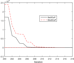
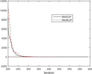
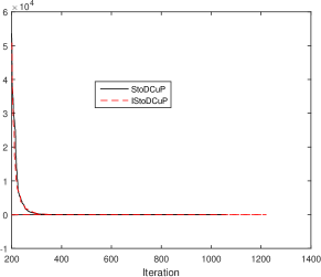
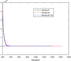
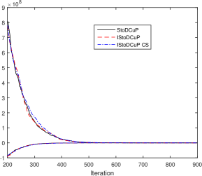
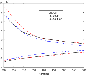
Same as SDDP, methods StoDCuP and IStoDCuP compute at each iteration a lower bound on the optimal value which is the optimal value of the first stage problem solved in the forward pass and upper bounds computed as SDDP by Monte-Carlo simulations, from iterations 200 on, using the last 200 forward scenarios. We also run the methods with the smoothed upper bounds used in [4, 14] which consists in using all previous forward passes to compute the upper bound but this implementation needed many more iterations to satisfy the stopping criterion for the large instances and the corresponding results will not be reported. We should also recall (see [8]) that for both IStoDCuP and StoDCuP the first stage problems are solved with high accuracy to get valid lower bounds from the optimal values of the first stage forward subproblems. The algorithms stopped when a relative gap of at most 0.1 was achieved for the first four instances while for the last two instances, the algorithms were run for 900 and 600 iterations, respectively.
As mentioned in Section 3.5, the cut selection methods proposed in [7, 10, 25] for SDDP can be directly applied to StoDCuP. The convergence of DDP, single cut SDDP, and multicut SDDP combined with these cut selection methods was proved in [7, 10]. For the three largest instances, we tested another cut selection strategy for the inexact variant IStoDCuP of StoDCuP, denoted by IStoDCuP CS, which consists, in the backward passes, from a given iteration and for the next iterations, to simultaneously add a new cut (computed at the trial points computed in the forward pass) for each cost-to-go function and to eliminate the oldest cut. As long as is not too large, we only eliminate, progressively, the cuts computed with loose accuracy (the cuts computed for the first iterations). Therefore, with this method, in the end of iterations , the number of cuts for each cost-to-go function is constant, equal to , and then from iteration on, one cut is added for each cost-to-go function at each iteration as in IStoDCuP if we choose one sampled scenario per forward pass. In our experiments, this cut selection strategy was run taking .
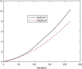
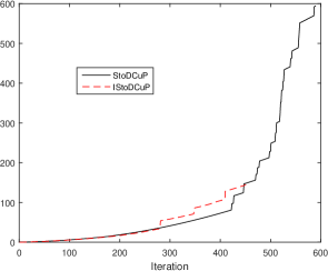
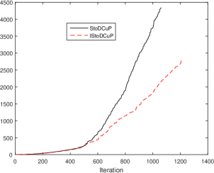
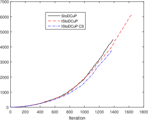
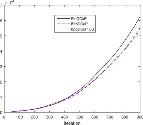
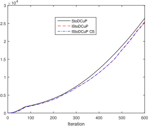
The evolution of the upper and lower bounds along the iterations of StoDCuP, IStoDCup, and IStoDCuP CS to solve the 6 instances is given in Figure 2 while the cumulated CPU time is given in Figure 3. All methods were implemented in Matlab and run on an Intel Core i7, 1.8GHz, processor with 12,0 Go of RAM. More precisely, the number of iterations and CPU time required to solve all instances is given in Table 3 and the bounds and cumulated CPU time for some iterations are given in Table 4.
We observe that the sequences of upper bounds tend to decrease, the sequences of lower bounds are increasing, and all these sequences converge to the same values for a given instance; which illustrates the validity of StoDCuP and IStoDCuP to solve a multistage stochastic nondifferentiable convex problem and is a good indication that both methods have been well implemented.
In all instances, at least one of the inexact variants of StoDCuP was quicker than StoDCuP and provided policies of similar quality. A general behavior we expect for IStoDCuP is to have quicker iterations but to need more iterations, as for instance , , , or a similar number of iterations, as for instances , , and (in this latter the number of iterations before gettting a gap smaller than 0.1 is 1376, 1387, and 1642 for respectively IStoDCuP CS, StoDCuP, and IStoDCuP (see Table 4)). However, it may happen that StoDCuP requires more iterations as for instance , , . The inexact variant with cut selection tested on the three largest instances allowed us to decrease the gap with respect to IStoDCuP while still being quicker than StoDCuP. It is also interesting to see that on the largest instance this inexact variant also yielded a much smaller gap than StoDCuP after completing the 600 iterations (see Table 4 and Figure 2).
| Iterations StoDCuP |
|
CPU time StoDCuP |
|
|||||
|---|---|---|---|---|---|---|---|---|
| 216 | 216 | 10.13 | 7.63 | |||||
| 586 | 451 | 597.2 | 148.4 | |||||
| 1061 | 1221 | 4345 | 2825 | |||||
| 1387 | 1376 | 4493 | 3784 | |||||
| 900 | 900 | 62 536 | 55 061 | |||||
| 600 | 600 | 26 414 | 25 276 |
 |
 |
 |
 |
 |
 |
 |
 |
 |
 |
 |
 |
| Iteration | UB IStoDCuP | UB StoDCuP | LB IStoDCuP | LB StoDCuP | Time IStoDCuP | Time StoDCuP |
|---|---|---|---|---|---|---|
| 10 | - | - | -36 424 | -15 037 | 0.09 | 0.16 |
| 200 | 24 109 | 16 990 | -29.3120 | -29.3123 | 6.98 | 8.91 |
| 210 | 282.4 | 73.9 | -29.3120 | -29.3123 | 7.57 | 9.67 |
| 216 | -26.99 | -27.34 | -29.3120 | -29.3123 | 7.63 | 10.13 |
| Iteration | UB IStoDCuP | UB StoDCuP | LB IStoDCuP | LB StoDCuP | Time IStoDCuP | Time StoDCuP |
|---|---|---|---|---|---|---|
| 10 | - | - | -98 584 | -82 872 | 0.29 | 0.35 |
| 210 | 6361.8 | 3889.3 | -19.023 | -17.44 | 20.6 | 18.5 |
| 451 | -14.97 | -13.58 | -16.27 | -16.25 | 148.4 | 144.6 |
| Iteration | UB IStoDCuP | UB StoDCuP | LB IStoDCuP | LB StoDCuP | Time IStoDCuP | Time StoDCuP |
| 10 | - | - | -440 000 | -352 310 | 0.65 | 0.72 |
| 400 | 9.68 | 13.84 | -12.09 | -12.58 | 140.9 | 151.7 |
| 800 | -6.01 | -8.69 | -10.83 | -10.85 | 1144.6 | 1897.2 |
| 1061 | -7.84 | -9.78 | -10.72 | -10.72 | 2166 | 4345 |
| 1221 | -9.78 | - | -10.69 | - | 2825 | - |
| Iteration | 600 | 1376 | 1387 | 1642 |
|---|---|---|---|---|
| UB IStoDCuP CS | -0.586 | -4.5343 | - | - |
| UB IStoDCuP | -1.6317 | -3.7448 | -3.7993 | -4.5153 |
| UB StoDCuP | -0.0327 | -3.9773 | -4.5648 | - |
| LB IStoDCuP CS | -5.5886 | -4.9595 | - | - |
| LB IStoDCuP | -5.6431 | -4.9584 | -4.9552 | -4.9078 |
| LB StoDCuP | -5.7420 | -4.9623 | -4.9591 | - |
| Time IStoDCuP CS | 525 | 3784 | - | - |
| Time IStoDCuP | 575 | 4106 | 4180 | 6178 |
| Time StoDCuP | 579 | 4424 | 4493 | - |
| Iteration | 400 | 600 | 900 |
| UB IStoDCuP CS | 2.5343e7 | 3.6465e5 | 143.2 |
| UB IStoDCuP | 2.1689e7 | 4.6095e5 | 338.7 |
| UB StoDCuP | 2.3785e7 | 3.0292e5 | -50.4 |
| LB IStoDCuP CS | -1.3343e6 | -4.0214e4 | -444.4 |
| LB IStoDCuP | -1.4643e6 | -5.0292e4 | -436.4 |
| LB StoDCuP | -0.9529e6 | -2.0954e4 | -428.9 |
| Time IStoDCuP CS | 8 534.6 | 21 166 | 56 082 |
| Time IStoDCuP | 7 946.7 | 21 557 | 55 061 |
| Time StoDCuP | 8 364.2 | 24 015 | 62 536 |
| Iteration | 400 | 500 | 600 |
|---|---|---|---|
| UB IStoDCuP CS | 1.943e8 | 1.1955e8 | 0.6321e8 |
| UB IStoDCuP | 2.2722e8 | 1.6320e8 | 1.2129e8 |
| UB StoDCuP | 2.3129e8 | 1.6563e8 | 1.0990e8 |
| LB IStoDCuP CS | -1.0060e8 | -0.5826e8 | -0.3522e8 |
| LB IStoDCuP | -1.6151e8 | -1.1376e8 | -0.6979e8 |
| LB StoDCuP | -1.5124e8 | -0.9974e8 | -0.6059e8 |
| Time IStoDCuP CS | 1.1254e4 | 1.7554e4 | 2.5276e4 |
| Time IStoDCuP | 1.1254e4 | 1.7618e4 | 2.5418e4 |
| Time StoDCuP | 1.2320e4 | 1.8689e4 | 2.6414e4 |
6. Conclusion
We introduced StoDCuP, a variant of SDDP which builds linearizations of some or all nonlinear constraint and objective functions along the iterations of the method, as well as an inexact variant of StoDCuP which is able to cope with approximate primal-dual solutions of the subproblems solved along the iterations. We have shown the convergence of StoDCuP and of Inexact StoDCuP for vanishing error terms .
Our numerical experiments have illustrated on a difficult nonlinear nondifferentiable multistage stochastic program that StoDCuP can be an alternative solution method to SDDP and that its inexact variant can converge quicker than StoDCuP. An interesting feature of the inexact variant is its flexiblity, able to cope with any approximate primal-dual solution to the subproblems, allowing to further study the impact of the calibration of error terms on the performance of Inexact StoDCuP. For DCuP, the calibration seems simpler, see for instance Remark 2 in [8] on the calibration of the error terms for Inexact DDP which also applies to Inexact DCuP.
Acknowledgments
The research of the first author was partially supported by an FGV grant, CNPq grants 401371/2014-0, 311289/2016-9, 204872/2018-9, and FAPERJ grant E-26/201.599/2014. Research of the second author was partially supported by CNPq grant 401371/2014-0.
References
- [1] E. D. Andersen and K.D. Andersen. The MOSEK optimization toolbox for MATLAB manual. Version 9.2, 2019. https://www.mosek.com/documentation/.
- [2] J.F. Benders. Partitioning procedures for solving mixed-variables programming problems. Numerische Mathematik, 4:238–252, 1962.
- [3] J.R. Birge. Decomposition and partitioning methods for multistage stochastic linear programs. Oper. Res., 33:989–1007, 1985.
- [4] L. Ding, S. Ahmed, and A. Shapiro. A python package for multi-stage stochastic programming. Optimization Online, 2019.
- [5] P. Girardeau, V. Leclere, and A.B. Philpott. On the convergence of decomposition methods for multistage stochastic convex programs. Mathematics of Operations Research, 40:130–145, 2015.
- [6] V. Guigues. Convergence analysis of sampling-based decomposition methods for risk-averse multistage stochastic convex programs. SIAM Journal on Optimization, 26:2468–2494, 2016.
- [7] V. Guigues. Dual dynamic programing with cut selection: Convergence proof and numerical experiments. European Journal of Operational Research, 258:47–57, 2017.
- [8] V. Guigues. Inexact cuts in Stochastic Dual Dynamic Programming. SIAM Journal on Optimization, 30:407–438, 2020.
- [9] V. Guigues. Inexact Stochastic Mirror Descent for two-stage nonlinear stochastic programs. Accepted for publication in Mathematical Programming, 2020. https://arxiv.org/pdf/1805.11732.pdf.
- [10] V. Guigues and M. Bandarra. Single cut and multicut SDDP with cut selection for multistage stochastic linear programs: convergence proof and numerical experiments. Computational Management Science, to appear. https://arxiv.org/abs/1902.06757.
- [11] V. Guigues, R. Monteiro, and B. Svaiter. Inexact cuts in SDDP applied to multistage stochastic nondifferentiable problems. arXiv, 2020. https://arxiv.org/abs/2004.02701.
- [12] V. Guigues and W. Römisch. Sampling-based decomposition methods for multistage stochastic programs based on extended polyhedral risk measures. SIAM J. Optim., 22:286–312, 2012.
- [13] V. Guigues and W. Römisch. SDDP for multistage stochastic linear programs based on spectral risk measures. Operations Research Letters, 40:313–318, 2012.
- [14] V. Guigues, A. Shapiro, and Y. Cheng. Duality and sensitivity analysis of multistage linear stochastic programs. Optimization OnLine, 2019.
- [15] V. Guigues, W. Tekaya, and M. Lejeune. Regularized decomposition methods for deterministic and stochastic convex optimization and application to portfolio selection with direct transaction and market impact costs. Optimization & Engineering, 21:1133–1165, 2020.
- [16] J.E. Kelley. The cutting plane method for solving convex programs. Journal of the SIAM, 8:703–712, 1960.
- [17] K.C. Kiwiel. An aggregate subgradient method for nonsmooth convex minimization. Mathematical Programming, pages 320–341, 1983.
- [18] K.C. Kiwiel. Proximity control in bundle methods for convex nondifferentiable minimization. Mathematical Programming, 46:105–122, 1990.
- [19] V. Kozmik and D.P. Morton. Evaluating policies in risk-averse multi-stage stochastic programming. Mathematical Programming, 152:275–300, 2015.
- [20] C. Lemaréchal. An extension of Davidon methods to non-differentiable problems. Mathematical Programming Study 3, pages 95–109, 1975.
- [21] C. Lemaréchal, A. Nemirovski, and Y. Nesterov. New variants of bundle methods. Mathematical Programming, 69:111–147, 1995.
- [22] R. P. Liu and A. Shapiro. Risk neutral reformulation approach to risk averse stochastc programming. arXiv, 2018. https://arxiv.org/abs/1901.01302.
- [23] M.V.F. Pereira and L.M.V.G Pinto. Multi-stage stochastic optimization applied to energy planning. Math. Program., 52:359–375, 1991.
- [24] A. Philpott and V. de Matos. Dynamic sampling algorithms for multi-stage stochastic programs with risk aversion. European Journal of Operational Research, 218:470–483, 2012.
- [25] A. Philpott, V. de Matos, and E. Finardi. Improving the performance of stochastic dual dynamic programming. Journal of Computational and Applied Mathematics, 290:196–208, 2012.
- [26] A. B. Philpott and Z. Guan. On the convergence of stochastic dual dynamic programming and related methods. Oper. Res. Lett., 36:450–455, 2008.
- [27] W.P. Powell. Approximate Dynamic Programming. John Wiley and Sons, 2nd edition, 2011.
- [28] R.T. Rockafellar. Convex Analysis. Princeton University Press, Princeton, 1970.
- [29] T. Rockafellar. Conjugate Duality and Optimization. No 16 in Conference Board of Math. Sciences Series, SIAM Publications, pages 1–79, 1974.
- [30] A. Ruszczyński and A. Shapiro. Conditional risk mappings. Mathematics of Operations Research, 31:544–561, 2006.
- [31] A. Ruszczyński and A. Shapiro. Optimization of convex risk functions. Mathematics of Operations Research, 31:433–452, 2006.
- [32] A. Shapiro. Analysis of stochastic dual dynamic programming method. European Journal of Operational Research, 209:63–72, 2011.
- [33] A. Shapiro, D. Dentcheva, and A. Ruszczyński. Lectures on Stochastic Programming: Modeling and Theory. SIAM, Philadelphia, 2009.
- [34] A. Shapiro and L. Ding. Periodical multistage stochastic programs. SIAM Journal on Optimization, 30:2083–2102, 2020.
- [35] R.M. Van Slyke and R.J.-B. Wets. L-shaped linear programs with applications to optimal control and stochastic programming. SIAM Journal of Applied Mathematics, 17:638–663, 1969.
- [36] Henry Wolkowicz, Romesh Saigal, and Lieven Vandenberghe. Handbook of Semidefinite Programming. Springer, 2000.
Data availability statement
All (simulated) data generated or analysed during this study can be obtained following the steps given in Section 5 of this article.
Appendix
To prove (3.77) and (3.90), we will need the following lemma (the proof of (ii) of this lemma was given in [5] for a more general sampling scheme and the proof of (i), that we detail, is similar to the proof of (ii)):
Lemma 6.1.
Assume that Assumptions (H0), (H1)-Sto, and (H2) hold for StoDCuP. Define random variables .
(i) Let , , , , and set
Let
and assume that . Define on the sample space the random variables , where and for
i.e., is the index of th iteration such that . Then random variables defined on sample space are independent, have the distribution of and therefore by the Strong Law of Large numbers we have
| (6.102) |
(ii) Let , , , and set
Let
and assume that . Define on the sample space the random variables , where and for
i.e., is the index of th iteration such that . Then random variables defined on sample space are independent, have the distribution of and therefore by the Strong Law of Large numbers we have
| (6.103) |
Proof: (i) Define on the sample space the random variables by
To alleviate notation ( being fixed), let us put , , For , we have
| (6.104) |
Observe that the event can be written as the union of events
Due to Assumption (H2) observe that random variable is independent of random variables , and therefore events and are independent which gives
| (6.105) |
where we have used the fact that and have the same distribution (from (H2)).
Next for , we have
By the same reasoning as above, the event
can be expressed in terms of random variables , and is therefore independent of event . It follows that
| (6.106) |
By induction this implies
| (6.107) |
which shows that random variables are independent.
The proof of (ii) is similar to the proof of (i).
Proof of (3.77) and (3.90). As in [5], we can now use the previous lemma to prove (3.77) and (3.90). Let us prove (3.77). By contradiction, assume that (3.77) does not hold. Then there is such that the set defined in Lemma 6.1 is nonempty. By Lemma 6.1, this implies that (6.102) holds. But due to (3.76), only a finite number of indices can be in (with corresponding variable being one) and therefore , which is a contradiction with (6.102).