Apricot
De-biasing convex regularized estimators and interval estimation in linear models
Abstract
New upper bounds are developed for the distance between and linear and quadratic functions of for random variables of the form . The linear approximation yields a central limit theorem when the squared norm of dominates the squared Frobenius norm of in expectation.
Applications of this normal approximation are given for the asymptotic normality of de-biased estimators in linear regression with correlated design and convex penalty in the regime for constant . For the estimation of linear functions of the unknown coefficient vector , this analysis leads to asymptotic normality of the de-biased estimate for most normalized directions , where “most” is quantified in a precise sense. This asymptotic normality holds for any convex penalty if and for any strongly convex penalty if . In particular the penalty needs not be separable or permutation invariant. By allowing arbitrary regularizers, the results vastly broaden the scope of applicability of de-biasing methodologies to obtain confidence intervals in high-dimensions. In the absence of strong convexity for , asymptotic normality of the de-biased estimate is obtained for the Lasso and the group Lasso under additional conditions. For general convex penalties, our analysis also provides prediction and estimation error bounds of independent interest.
1 Introduction
Consider the linear model
| (1.1) |
with an unknown coefficient vector , a Gaussian noise vector , and a Gaussian design matrix with iid rows independent of . We assume throughout the sequel that is invertible. The paper develops confidence intervals for from a given regularized initial estimator , using a technique referred to as de-biasing: a correction to the initial estimate in the direction is constructed so that the “de-biased” estimate can be used for inference about .
1.1 Regularization induces bias
If is invertible, the unregulated least-squares estimate is unbiased, that is, . On the other hand, if the square loss is regularized with an additive penalty,
| (1.2) |
for penalty functions commonly used in high-dimensional statistics such as for (Lasso) or for (ridge regression), then is biased.
For ridge regression , this bias can be quantified explicitly when as a shrinkage to the origin. Let be the SVD of with and . By rotational invariance, is independent of and uniformly distributed in the unit sphere in p. Thus, with being the Marchenko-Pastur law,
The Lasso penalty also introduces bias. For example, for deterministic orthonormal designs, the Lasso estimator of the coefficient is the soft-thresholding of which is again biased toward the origin. For Gaussian designs with and in an average sense, the Lasso is approximately the soft-thresholding of with certain under proper conditions [1]. Thus, with , the squared bias of the Lasso, , is expected to have no smaller order than the lower bound for its risk [3, Theorem 3.1]. Alternative approaches were proposed to remove or reduce the bias of the Lasso for strong signals, e.g., by using concave penalty functions (e.g., SCAD [21], MCP [44]) or iterated hard thresholding algorithms [11]. These approaches yield an error term of the order where for some constant [22, 30], alleviating the bias of the Lasso for large coefficients at typical penalty levels .
De-biasing the Lasso, asymptotic normality and confidence intervals
If the goal is the estimation of a single scalar parameter in a predetermined direction instead of the full vector , it is possible to correct the bias of the Lasso and to construct confidence intervals for : there is already a vast literature on asymptotic normality of de-biased estimates in sparse linear regression for the Lasso [47, 42, 23, 24, 8, 25, 29, 6, among others]. In this literature is usually the -th canonical basis vector and the scalar parameter of interest. Given the Lasso as an initial estimator of , the idea is to add a de-biasing term to achieve asymptotic normality which then yields confidence intervals for . If in (1.1), several de-biased estimators have been proposed and their asymptotic normality hold under certain rate conditions on . The earliest works on this topic [47, 42, 23, 8] provide asymptotic normality results in the regime . When indeed holds, the de-biasing constructions in these papers are all first order equivalent to each other, and under normalization to
| (1.3) |
where and . While these works do not assume known and construct an estimated score vector for , the impact of using can be absorbed into the remainder in (1.3) with . The direction and the de-biasing correction in (1.3) have a natural semi-parametric interpretation [45]. Viewing as the function , the Fischer information for the estimation of in (1.1) is , and the direction above is the only with
| (1.4) |
such that is also the Fischer information in the one-dimensional submodel . For this reason the line is referred to as the least-favorable one-dimensional submodel for the estimation of . The normalization (1.4) ensures that and with , so that (1.3) replaces the initial with its one-step correction , where maximizes the likelihood in the least-favorable submodel. We refer to [9] for a systematic study of this semi-parametric perspective.
If and is unknown with bounded spectrum, the minimax estimation error of the form diverges for any estimator [14]. This rules out asymptotic normally results at the adjusted rate if and no further assumption is made on . However, if is known, (1.3) holds with , providing asymptotic normality for sparsity levels up to logarithmic factors, cf. [6, Corollary 3.3]. Similarly, [25, Theorem 3.8] provides (1.3) with a canonical basis vector and . Already in the regime , the arguments of [25, 6] differ significantly from the - Hölder inequality argument of [47, 42, 23, 8]: while these earlier works prove asymptotic normality with a remainder term of order , [25, 6] analyze explicitly the smaller order terms hidden in this remainder.
For , the de-biasing correction in (1.3) needs to be modified:
| (1.5) |
with and , cf. [6, Theorem 3.1]. For the difference from (1.3) is the replacement of in the de-biasing correction with to amplify it by a factor . This modification is required as soon as up to logarithmic factors [6, Section 3]. These asymptotic results for are amenable to the lack of knowledge of : in this case estimation of is possible when is sufficiently sparse, see [25] if the direction of interest is canonical basis vector and [6, Section 2.2] for arbitrary direction . These results [25, 6] for and correlated are so far restricted to random Gaussian designs.
Inflated asymptotic variance for non-vanishing prediction error
In the results discussed so far for the Lasso, or stronger conditions are required for asymptotic normality, and the asymptotic variance of is . The condition implies the consistency of the Lasso in prediction and estimation thanks to error bounds of the form [46, 34, 7, 6]. It turns out that the asymptotic variance of is larger than if does not vanish; this is the situation studied in the present work. The literature on asymptotic normality of de-biased estimates in the regime
| (1.6) |
for constants is more scarce. In this regime where and are all of the same order, [24, 29] provide asymptotic normality results for the de-biased Lasso (1.5) in the estimation of (canonical ) in the isotropic Gaussian design. In these works, the asymptotic variance of equals a constant satisfying the system of two nonlinear equations in [1] and [29, Proposition 3.1,Theorem 3.1]. The constant is related to the residual sum of squares [29, Corollary 4.1] and out-of-sample error [29, Theorem 3.2] as in
where denotes convergence in probability. These results for highlight that the asymptotic variance is strictly larger than when are of the same order as in (1.6). This phenomenon in the regime (1.6) is generic: for instance the asymptotic variance is also larger than for all permutation-invariant penalty functions [15, Proposition 4.3].
In this regime where and are of the same order, [20, 18] proved asymptotic normality and characterized the variance for unregularized -estimators. For -estimators a de-biasing correction is unnecessary due to the absence of regularization, and a rotational invariance argument reduces the problem of correlated designs to a corresponding uncorrelated one [20, Lemma 1]. However, this rotational invariance is lost in the presence of a penalty such as the -norm. New techniques are called for to analyse the asymptotic behavior, in the regime (1.6) and under correlated designs, of estimators that are not rotational invariant. More recently, the Approximate Message Passing techniques used in [24, 18] were used to obtain similar results in logistic regression [36]; but again, these techniques cannot handle the Lasso penalty for correlated design. A more detailed comparison with these works is made in Section 3.8. To our knowledge, there is no previous asymptotic normality result for de-biased estimates in the regime (1.6) for correlated designs in the presence of a penalty not depending on (i.e., in situations where rotational invariance does not hold). A main goal of the paper is to fill this gap. Available techniques that tackle the regime (1.6) assume, in addition to uncorrelated design, that the penalty is invariant under permutations of the coefficients [1, 29, 15, 13] and that the empirical distribution of the true converges to some prior distribution. A second goal of the present paper is to show that asymptotic normality of de-biased estimates can be obtained beyond the Lasso and beyond permutation-invariant penalty functions, without imposing the convergence of the empirical distribution of the normalized coefficients .
1.2 A general construction of de-biased estimators
This section describes a general approach to systematically construct de-biased estimates in the linear model (1.1) where has iid rows. Our goal is to construct confidence intervals for the one-dimensional parameter . Consider an initial estimator , viewed as a function of , i.e., and assume that this function is Fréchet111 Although the Fréchet derivative is the usual definition of derivative in finite dimension, we write Fréchet to emphasize that the derivative is linear. Linearity may fail for weaker notions such as Gateaux differentiability. differentiable. For a given observed data from the linear model (1.1) and a Fréchet differentiable at , there exist uniquely matrices and such that
| (1.7) | ||||
for all . With , if the partial derivatives of at the observed data are and then (1.7) implies and for canonical basis vectors and . The derivatives of and the matrices and can be computed by only looking at the observed data , for instance by finite difference schemes.
Next, consider the function defined as
If is differentiable at then is differentiable as well. By the product and chain rules
| (1.8) |
If the partial derivatives of are and , the second line of the previous display is equivalently rewritten as
for each canonical basis vector .
Observe that the arguments of are centered and jointly normal random variables and their correlations are computed explicitly, e.g., , with basis vectors . One version of Stein’s formula, also known as Gaussian integration by parts, is provided that the function is differentiable and that are centered jointly normal random variables, provided the existence of the expectations [37, Appendix A.4]. We leverage this version of Stein’s formula to obtain an unbiased estimating equation involving only one unknown parameter, the scalar of interest. For we find if while and so that by reading the partial derivatives in (1.8),
| (1.9) | |||||
| (1.10) |
Summing over and using , we find that
To transform this equation into a form representative of the results of the paper, define the scalars and by
| (1.11) |
The notation underlines that has the interpretation of degrees-of-freedom of the estimator in Stein’s Unbiased Risk Estimate (SURE) [33]: regarding as an estimate of in the Gaussian sequence model with observation , the quantity is an unbiased estimate of the in-sample error . With this notation, we obtain the unbiased estimating equation
| (1.12) |
where the only unobserved quantity inside the expectation is , the scalar parameter we wish to estimate. In the above application of Stein’s formula, was chosen on purpose so that appears in (1.9) only through thanks to . Note that replacing in (1.9) by for any not proportional to brings a scalar projection of different from : this shows the unique role of the random vector to derive an unbiased estimating equation for . It is notable that the direction coincides with the least-favorable direction described around (1.4). Equation (1.12) is obtained for an arbitrary initial estimator provided that its derivatives with respect to exist and the integrability conditions hold to ensure existence of the expectations involved. From (1.12), the method of moments suggests to estimate with which resembles (1.5) for the Lasso for and under the normalization .
It is useful at this point to specialize the above derivation to an estimator for which all derivatives can be computed explicitly. For Ridge regression with penalty for some , and
| (1.13) | ||||
| (1.14) |
Indeed, the derivatives of exist as it is the composition of elementary differentiable functions. Differentiation with respect to is straightforward as is linear in , while in order to compute we proceed by setting with . Differentiation of the KKT conditions at provides the directional derivative . This gives (1.13). It follows from (1.13) that and for the quantities in (1.11) (for , note the fortuitous cancellation of the term ). For the Lasso similar differentiability formulae are derived in [6]. It is however, unclear how to obtain closed form formulae for the derivatives of for an arbitrary convex penalty in (1.2).
We now set up some notation that will be useful for the rest of the paper, and derive again the unbiased estimating equation (1.12) using this new notation. Define
| (1.15) |
The normalizing constant in is such that holds so that the expression (1.15) for coincides with the direction of the least-favorable submodel discussed around (1.4). The vector is independent of by construction as are jointly normal and uncorrelated. This follows by noting that has iid entries and
for the unit vector as by construction of matrix is the orthogonal projection onto . We summarize this as
| (1.16) |
For brevity, we assume in the sequel and without loss of generality that the direction of interest is normalized such that
| (1.17) |
By definition of and , the normalization (1.17) gives .
Conditionally on , define the function by
| (1.18) |
By (1.16) and the independence of and , the conditional expectation given can be written as integrals against the Gaussian measure of , e.g.,
since . As we argue conditionally on , we omit the dependence on and write simply . Since and ,
The gradient with respect to , holding fixed, can be computed by the product rule and the chain rule via (1.8):
| (1.19) |
We adopt the usual convention that the gradient of a vector valued function is the transpose of its Jacobian. Computing the directional derivative of in a direction requires considering difference of an expression at minus the same expression at , dividing by and taking the limit as ; this is equivalent to considering the difference of an expression at with minus the same expression at , dividing by and taking the limit as .
Taking the trace of (1.19) and by definition of and in (1.11), the identity
| (1.20) | |||||
holds where . Since by Stein’s formula [33], this provides the unbiased estimating equation (1.12). Reasoning conditionally on , using Stein formulae with respect to involving conditional expectations given and gradients of the form holding fixed will be a recurring theme throughout the paper. In this context, the function itself depends on as in (1.18), although the dependence on is omitted for brevity.
In order to construct confidence intervals using the unbiased estimating equation (1.12), one may hope that the quantity (1.20) above is well behaved—ideally, approximately normal with mean zero and a variance that can be consistently estimated from the observed data. By the Second Order Stein’s formula in Proposition 2.1 below, which was already known to Stein [33, (8.6)] in a different form, the conditional variance of (1.20) given is
where denotes the conditional expectation with respect to given and denotes the conditional variance given . The gradient in (1.19) and the unbiased estimate of only depend on the unknown parameter of interest and observable quantities, and is quadratic in .
Assume now we are in an ideal situation in the sense that both conditions below are satisfied: (i) The quantity (1.20) is approximately normally distributed conditionally on , and (ii) is a consistent estimator of (1.2), the conditional variance of the random variable (1.20). Then the set of for which the inequality
| (1.22) |
is satisfied is an -confidence interval, where . Solving the corresponding quadratic equality gives up to two solutions that are such that (1.22) holds with equality. These two solutions implicitly depend on the observables
and the derivatives of . If the coefficient of in the left hand side of (1.22) is positive, (i.e., if the leading coefficient of (1.22), seen as a polynomial in with data-driven coefficients, is positive), a confidence interval for is then given by
| (1.23) |
We will show in the discussion surrounding (3.33) below that the dominant coefficient is positive and that the confidence interval is indeed of the above form if is a convex penalized estimator. Although a variant of the above construction was briefly presented in [5, Section 6] (there, the function is used), important questions remain unanswered to prove the validity of the general confidence interval in (1.23) and its applicability to commonly used regularized estimators.
1.3 The rest of the paper is organized as follows
Section 2 develops an bound between and for random variables of the form where . Section 3 uses this normal approximation to show the asymptotic normality of (1.20) and proves the consistency of the variance estimate in (1.2) in the regime where and are of the same order in the linear model (1.1) with correlated design. Section 4 provides closed-form formulas to apply the results in Section 3 to the Lasso, the group Lasso and twice continuously differentiable penalty functions. Section 5 contains the proofs of the results in Section 3. Appendix A provides a technical lemma on the integrability of smallest eigenvalue of Wishart matrices, Appendix B provides the proofs of the asymptotic normality results for the Lasso and group Lasso when , and Appendix C contains the proofs of the derivative formulae for the group Lasso.
1.4 Notation
For two reals , let , and . Let be the identity matrix of size , e.g. . For any , let be the set . Let be the Euclidean norm and the norm of vectors for any , so that . Let be the operator norm of matrices and the Frobenius norm. Let be the smallest eigenvalue of a symmetric matrix . We use the notation for the canonical scalar product of vectors in n or p, i.e., for two vectors of the same dimension. For any event , denote by its indicator function. The unit sphere is . Convergence in distribution is denoted by and convergence in probability by . Throughout the paper, denote positive absolute constants, positive constants depending on only, and on only.
For any vector and set , the vector is the restriction . For any matrix with columns and any subset , let be the matrix composed of columns of indexed by . If is a symmetric matrix of size and , then denotes the sub-matrix of with rows and columns in , and is the inverse of . For any square matrix , let be its symmetrization giving the same quadratic form.
For a vector valued map with coordinates , the gradient is the matrix with columns . Thus, is the transpose of the Jacobian of and if each coordinate is Fréchet differentiable at . For deterministic matrices , . For in (2.1), and the divergence is .
2 Normal approximation in Stein’s formula
We develop in this section normal approximations for random variables of the form
| (2.1) |
for which Stein’s formula [33] states , where is standard normal and . We establish bounds for the linear and quadratic approximations of and construct consistent variance estimates in the related CLT.
Throughout this paper, the -th coordinate of is a function and its weak gradient is denoted by . Similarly, the weak derivative of is denoted by . We refer to [12, Section 1.5] for definitions of weak differentiability. For the application to asymptotic normality of de-biased estimates in Section 3, the functions we will consider are locally Lipschitz. By Rademacher’s theorem, locally Lipschitz functions are Fréchet differentiable almost everywhere, which is stronger than the existence of directional derivatives in all directions. In this case the weak derivatives agree with the classical partial derivatives almost everywhere. As far as the application in Section 3 is concerned, the reader unfamiliar with weak differentiability may consider the additional assumption that is locally Lipschitz in the following results and replace weak derivatives with classical derivatives. The variance of (2.1) is given by the following proposition.
Proposition 2.1.
The above result, in the twice differentiable case, was known to Stein [33, Eq. (8.6)]. If is twice differentiable, the result follows by a sequence of integration by parts. The differentiability requirement was relaxed to only once weakly differentiable in [5] where statistical applications of this formula to such once differentiable are discussed.
2.1 Linear approximation
The goal of the present section is to derive normal approximations and CLT for the random variable (2.1). The intuition is as follow. We are looking for linear approximation of the random variable (2.1), of the form for some deterministic . We rewrite (2.1) as
| (2.3) |
The remainder term above is mean-zero with second moment equal to by Proposition 2.1. This second moment is minimized for , hence gives the best linear approximation of in (2.1). The following result provides conditions on under which the remainder term is negligible in (2.3).
Theorem 2.2.
Let and be a function , with each coordinate being squared integrable and weakly differentiable with squared integrable gradient, i.e. . Then satisfies
| (2.4) |
with , deterministic real and
| (2.5) |
where . Consequently, for .
A direct consequence of Theorem 2.2 is . Inequality (2.4) provides an upper bound on the 2-Wasserstein distance between and . When , it gives a stronger form of the CLT in addition to the Kolmogorov distance bound in Theorem 2.2. The theorem follows from Proposition 2.1 and an application of the Gaussian Poincaré inequality.
Proof of Theorem 2.2.
Define then and
where and . By Proposition 2.1 applied to and a bias-variance decomposition,
thanks to . Thus, (2.4) follows from the definition of in (2.5). Moreover, by the Gaussian Poincaré inequality and for . Hence, with , , and we have
thanks to another Gaussian Poincaré inequality for the last inequality. Finally, holds for all which proves .
For any , by Markov’s inequality since the standard normal pdf is uniformly bounded by . Hence, with , the above and a similar argument on provide the Kolmogorov distance bound. ∎
Normal approximation results such as Theorem 2.2 are flexible tools as they let us derive asymptotic normality results by mechanically computing gradients: By Theorem 2.2 it suffices to show that the expectation of is negligible compared with that of to obtain . Normal approximations involving derivatives have been studied for random variables with the more general form for differentiable functions . The Second Order Poincaré inequality of [16] bounds the total variation distance of to the Gaussian distribution using the first and second derivatives of : [16, Theorem 2.2] specialized to with states that
| (2.6) |
where , , and . Above, denote the gradient and Hessian matrix of . Inequality (2.6) provides a CLT for provided that the moments of the derivatives and are negligible compared to the variance . Inequality (2.6) has been successfully applied to derive asymptotic normality of unregularized -estimators when and the -estimation loss is twice differentiable [28]. However, the (2.6)-based approach is not applicable for regularized estimators such as the Lasso and group Lasso that are only once differentiable functions of . In fact, by Proposition 4.1 below, the Lasso is not twice differentiable as is integer-valued. In Theorem 2.2, while already involves the derivatives of through the divergence, the ratio that appears in the upper bound (2.5) only involves and its gradient ; the second derivatives of need not exist. Section 3 uses Theorem 2.2 to provide asymptotic normality for de-biasing estimators that are only once differentiable.
Variance estimate
It follows from Theorem 2.2 that random variables of the form (2.1) are asymptotically normal under the condition , or under a somewhat stronger but more explicit condition as in (2.5). The following theorem provide consistent estimates of .
Theorem 2.3.
Proof of Theorem 2.3.
2.2 Quadratic approximation
The decomposition (2.3) is especially useful if the linear part with is a good approximation for . In some cases, e.g., if for some square deterministic matrix , the decomposition (2.3) is uninformative. It is then natural to look for the best quadratic approximation of in the sense of the orthogonal projection to
where and are subspaces orthogonal to each other.
The calculation in (2.4) for is generic in the following sense. If is the projection of a random variable in then the sine of the -angle between and is and
| (2.10) |
holds for some deterministic real . Indeed, take with being the -angle between and , so that (2.10) becomes as in the proof of Theorem 2.2.
The next result extends Theorem 2.2 to the quadratic projections to and , and also gives Theorem 2.2 the interpretation as the projection to .
Theorem 2.4.
Let , satisfy the assumption of Theorem 2.2, and . For and let . Let and . Then, is the projection of to and
| (2.11) | |||||
| (2.12) |
Consequently, is the projection of and to with and is the projection of and to with .
For the projection of to , satisfies and under the condition ,
| (2.13) |
For the projection of to , satisfies and under the condition ,
| (2.14) |
Proof of Theorem 2.4.
The function has gradient . Application of the Second Order Stein’s formula in Proposition 2.1 to yields
The first term is . By Stein’s formula and the linearity of the trace, we have
We also have so that
For the second term, using that we get
Due to for , it follows that
The optimality of and follows, so that is the projection of to . Also, the first line above gives the formula of in (2.11), and the second line gives the formulas for the variances of and . The upper bound in (2.11) follows from thanks to the Gaussian Poincaré inequality. Inequality (2.11) is equivalent to
which provides and by bounding from above the denominator in and .
For (2.13), we write with iid , where and with the eigenvalue decomposition . Assume without loss of generality that is non-increasing in and that satisfies . The condition on the left-hand side of (2.13) implies that the integer satisfies and , so that
Assuming that for some by extracting a subsequence if necessary, implies so that the second term above is independent of the first and approximately by the Lyapunov CLT when . This proves that the LHS of (2.13) implies the RHS. Conversely, assume the asymptotic normality on the RHS so that . Let and . As is an independent component of the sum, for any along a subsequence with , we must have because by the Cramér-Lévi theorem and for some . As are arbitrary, this gives . ∎
Variance estimate: quadratic case
Theorem 2.4 provides the quadratic normal approximation of under the condition with
| (2.15) |
where is defined using the upper bound established in (2.11) in the denominator on the right-hand side of (2.15).
Theorem 2.5.
Let and be as in Theorem 2.4 and . Then,
| (2.16) |
with and . Consequently, under the conditions and ,
| (2.17) |
It follows from the Second Order Stein formula in Proposition 2.1 that is an unbiased estimator of . Moreover, when , and are all equivalent to their symmetric counterparts, , and , the condition for (2.17) holds if and only if for the quantities in (2.15) and (2.13). The proof is given in Appendix D.
3 De-biasing general convex regularizers
Our main application of the normal approximation in Theorem 2.2 concerns de-biasing regularized estimators of the form
| (3.1) |
for convex in the linear model (1.1). Throughout, let be the error vector, be a direction of interest, be the target of statistical inference, and , and be as in (1.15) so that (1.16) holds.
3.1 Assumption
We say that is -strongly convex with respect to the norm if its symmetric Bregman divergence is bounded from below as
| (3.2) |
for some . Here the interpretation of (3.2) is its validity for all choices in the sub-differential and . Condition (3.2) holds for any convex for . If is twice differentiable, (3.2) holds if and only if is a lower bound for the Hessian of . However, (3.2) may also hold for non-differentiable , e.g. the Elastic-Net penalty with . Our results require the following assumption.
Assumption 3.1.
Note that if (3.2) holds for it also holds for and we may thus assume without loss of generality. Strongly convex objective functions admit unique minimizers. Since implies (cf. Appendix A) and the objective function of the optimization problem (3.1) is -strongly convex, Assumption 3.1 grants almost surely the existence and uniqueness of the minimizer (3.1).
3.2 Gradient with respect to and effective degrees-of-freedom
Consider a penalized estimator (3.1) viewed as a function . For every , the map is 1-Lipschitz (cf. Proposition 5.3). By Rademacher’s theorem, for almost every there exists a unique matrix such that
| (3.3) |
as in (1.7), i.e., is the gradient of the map . Furthermore is symmetric with eigenvalues in ; See Proposition 5.3 for the existence of and its properties. While existence of was assumed in (1.7) in the introduction, for penalized estimators (3.1) the matrix provably exists for almost every by Proposition 5.3.
Table 1 provides closed-form expressions of for specific penalty functions . The proofs of these closed-form expressions will be given in Section 4. An advantage of defining as the Fréchet derivative of the Lipschitz map is that this definition applies to any convex penalty , even though for arbitrary penalty we are unable to provide a closed-form expression for . Finally, define the effective degrees-of-freedom of by
| (3.4) |
as in (1.11). Because is symmetric with eigenvalues in (cf. Proposition 5.3), holds almost surely. The matrix and the scalar play a major role in our analysis.
| Penalty | Justification | |
|---|---|---|
| (Lasso) | [40], Proposition 4.1 | |
| (Ridge) | (1.13), Section 4.1 | |
| (Elastic-Net) | [40, (28)], [5, §3.5.3] | |
| (group Lasso (3.36)) | [41], Proposition 4.2 | |
| twice continuously differentiable | Section 4.1 | |
| arbitrary convex function | symmetric with eigenvalues in | Proposition 5.3 |
3.3 Approximation for and the de-biased vector
Consider, for a fixed value of the function given by
| (3.5) |
For brevity we will often omit the dependence on of as discussed after (1.18). The Fréchet gradient , where it exists, is uniquely defined by
| (3.6) |
and the divergence by . If with , then (3.6) is equivalent to
| (3.7) |
By Stein’s formula, we have conditionally on that almost surely
| (3.8) |
As in (1.20) for the general case discussed in the introduction, (3.8) gives an unbiased estimating equation for . The next lemma provides an expression for .
Lemma 3.1.
Let Assumption 3.1(i) be fulfilled, and be as in (3.3). Then,
| (3.9) |
satisfies (3.6) for some random almost surely. If additionally then
| (3.10) |
| Penalty | Vector in Lemma 3.1 | Justification |
|---|---|---|
| (Lasso) | [6], Proposition 4.1 | |
| (Ridge) | Section 4.1 | |
| (group Lasso (3.36)) | Proposition 4.2 | |
| twice continuously differentiable | Section 4.1 |
Lemma 3.1 is proved in Section 5.1. Although we do not use this fact in any results, we mention here in passing that vector in (3.9) is linear in in the sense that can be chosen of the form for some matrix . Indeed, the proof of Lemma 3.1 shows that the map is Fréchet differentiable at almost every point by Rademacher’s theorem. At such a point, with , , the linear combination and the perturbed design matrix , linearity of the Fréchet derivative implies that
where and denote the from (3.9) for and respectively. Hence with , (3.9) holds for . This proves that is linear in , i.e., it is of the form for some matrix . One way to construct explicitly is the following: define the -th column of as the vector corresponding to where is the -th canonical basis vector. The linearity proved above for any linear combination then implies that (3.9) holds for for any . Inequality (3.10) provides an upper bound on the operator norm of . Linearity of with respect to and explicit matrices can be seen for some penalty functions in Table 2.
By taking the trace of (3.9), we obtain almost surely under Assumption 3.1
| (3.11) | |||||
| (3.12) | |||||
| (3.13) |
for
| (3.14) |
In the present context of the regularized estimator in (3.1) with its effective degrees-of-freedom defined in (3.4) and under Assumption 3.1, the quantities , , in the previous display coincide with the random variables with the same name in (1.20). By (3.8), equality holds so that
| (3.15) | |||||
| (3.16) |
by taking expectations in (3.11). This provides a first evidence that the correction indeed removes the bias, at least after multiplication of by . Since under the normalization (1.17), the unbiased estimating equation (3.15) is the specialization of (1.12) from the introduction to the penalized estimator (3.1), for which we have the gradient expression (3.9) in terms of and . If is given by (3.1), by identifying the terms in (1.20) and (3.11) we see that the random variable defined in (1.11) of the introduction is here with given by Lemma 3.1. The following lemma shows that this term is negligible.
Lemma 3.2.
Under Assumption 3.1 there exists with and
| (3.17) |
The proof is given in Section 5.6. Since , inequality (3.17) implies . This motivates the definition
| (3.18) |
The de-biased estimate in direction is obtained from in (3.14) by dropping the smaller order term . By Slutsky’s theorem, (3.17) implies
| (3.19) |
for any candidate limiting distribution . As , this suggests that the simpler correction in (3.18) also corrects the bias of . By Prohorov’s theorem, there exists a subsequence and limiting distribution such that (3.19) holds in this subsequence. While is mean-zero as has mean zero and variance one, has variance at most one by Fatou’s lemma. However, the normality of is unclear at this point.
To obtain more precise information on the limiting distribution and the deviations of , the next subsections build estimate of its variance and derive asymptotic normality results by showing that for most directions . The next result provides a loose data-driven upper bound on the error .
Theorem 3.3.
Theorem 3.3 is proved in Section 5.7. If then is of the same order as the width of confidence intervals based on the least-squares estimator as while remains fixed. Theorem 3.3 shows that under this mild additional assumption on the prediction error , the second term in (3.18) indeed corrects the bias, achieving .
3.4 Variance estimates
By Proposition 2.1, the conditional variance can be written as for
| (3.21) |
We allow the variance estimate to depend on the unknown as the resulting pivotal quantity, via (3.11), would depend on anyway. While itself can be used to estimate , its sign is unclear. The following simplified version of it, obtained by removing the smaller order terms in ,
| (3.22) | ||||
is non-negative. This follows from Proposition 5.3 since is almost surely positive semi-definite. Lemma 3.4 below shows that the relative bias converges to 0 in probability, i.e., is asymptotically unbiased for .
Lemma 3.4.
Under Assumption 3.1 there exists with and
| (3.23) |
An alternative variance estimate, that does not depend on the unknown parameter , is given by replacing in by the point estimate with in (3.18):
| (3.24) |
The next lemma provides and that is also asymptotically unbiased in the sense . Lemmas 3.4 and 3.5 are proved in Section 5.6.
Lemma 3.5.
Under Assumption 3.1 there exists with and
| (3.25) |
3.5 Asymptotic normality of de-biased estimates
Throughout this section, denotes the standard normal cdf. For a given penalty function , we define the deterministic oracle and its associated noiseless prediction risk by
| (3.26) |
Our first result provides asymptotic normality of the de-biased estimate when the error of in direction is negligible compared to .
Theorem 3.6.
Let Assumption 3.1 be fulfilled. Let be as in (3.18). Then, for any with such that ,
where denotes any of the four quantities: , , or .
Theorem 3.6 is proved in Section 5.7. The theorem, as well as its variants below, are obtained by applying Theorem 2.2 conditionally on to the function in (3.5). This argument relies on the normality of conditionally on and thus the Gaussian design assumption. Here is an outline. Define
| (3.27) |
where and are the conditional expectation and conditional variance given . It is sufficient to show that in order to prove asymptotic normality of by Theorem 2.2 and of by Theorem 2.3 since satisfies for the in Theorems 2.2 and 2.3. The proof makes rigorous the following informal bound:
for some constant , by establishing a lower bound on for the denominator (Lemmas 5.6, 5.4 and 5.7), and by showing that the rank one term in (3.9) is negligible in the numerator. Finally, always holds by Proposition 5.3 and is shown to be uniformly integrable, so that the assumption grants . The next two results identify directions such that holds.
Theorem 3.7.
There exists an absolute constant such that the following holds. Let Assumption 3.1 be fulfilled, be as in (3.18). Then for any increasing sequence (e.g., ), the subset
| (3.28) |
of the unit sphere in p has relative volume and
| (3.29) |
where denotes any of the four quantities: , , or . Furthermore, with the -th canonical basis vector and , the asymptotic normality in (3.29) uniformly holds over at least canonical directions in the sense that has cardinality .
Theorem 3.7 is proved in Section 5.7. For a given sequence of directions , if then it follows by choosing that for the in (3.28) so that (3.29) implies that asymptotic normality holds for this sequence of . In other words, asymptotic normality holds for all such that . Thus a sequence of directions for which asymptotic normality does not follow from Theorem 3.7 is a sequence such that does not vanish, i.e., the squared error in direction carries a constant fraction of the full prediction error . Such direction must thus be very special, which is embodied by the exponentially small bound on the relative volume .
Theorem 3.8.
Under Assumption 3.1 there exists with and
| (3.30) |
If additionally is a seminorm then always holds by properties of the subdifferential of a norm. Consequently, if then and the conclusions of Theorem 3.6 hold.
Theorem 3.8 is proved in Section 5.7. The first part of the theorem says that the estimation error is essentially up to an error term of order , so that if and only if . Combined with the fact that is bounded away from 0 by Lemma 5.4, this implies that if and only if . The last part of the theorem relies on the property for any norm where is the subdifferential of at . This property also holds if is a semi-norm, however it is unclear how to extend the last part of the above theorem if is not a semi-norm.
For the Lasso, the penalty function is and condition becomes . Typically, the tuning parameter is chosen as with [10, among others] or [35, 27, 7, 22, 2], where . For such choices, the condition can be written as and since , a sufficient condition is . If is a vector of the canonical basis, the normalization (1.17) gives and is the norm of the -th column of . The condition allows, for instance, the -th column of to have constant entries. This assumption is weaker than that of some previous studies; for instance [25] requires for . The following example illustrates the benefit of picking a proper penalty level .
3.6 Confidence intervals
Theorems 3.6, 3.7 and 3.8 are valid for any choice of the variance estimate among in (3.22) and in (3.25) for directions such that holds. For such direction , the choice leads to the narrowest confidence interval for , namely
| (3.31) |
where denotes the interval , and is the de-biased estimator in (3.18). The choice leads to intervals with larger multiplicative coefficient for , namely
| (3.32) |
has probability converging to for directions satisfying any of the above theorems. For such directions, the choice justifies confidence intervals of the form (1.23) as
| (3.33) |
holds with probability converging to . Given the expression for in (3.22), the left-hand side of (3.33) is a quadratic polynomial in with dominant coefficient . Since almost surely by properties of in Proposition 5.3 and for some constant with probability approaching one by Lemma 5.4, in the same event the dominant coefficient is positive. The intersection of events (3.33) and has probability converging to and in this event, where are the two real roots of the left-hand side of (3.33) as a quadratic function of .
3.7 Variance spike
One can pick any choice among the three variance estimates in Theorem 3.6 because it assumes and this limit in probability implies both and . These limits in probability to 1 are made rigorous by (3.25) and by the lower bound obtained from Lemmas 5.7, 5.4 and 5.6 as explained in (5.43) of the proof.
The reason that the estimates and were introduced is that the simpler estimate is not asymptotically unbiased for for directions such that does not converge to 0 in probability: While the relative bias of and provably converges to 0 in Lemma 3.4 and (3.25) for all directions , the same cannot be said for the simpler estimate .
Theorem 3.9.
Let Assumption 3.1 be fulfilled. Then the following are equivalent:
-
(i)
,
-
(ii)
,
-
(iii)
,
-
(iv)
,
-
(v)
,
-
(vi)
,
-
(vii)
.
Theorem 3.9 is proved in Section 5.6. It shows that for the directions such that does not hold, e.g., directions such that the error is of the same order as the average squared residual (see Lemma 5.2 in Section 5.2), the simpler estimate fails to account for a non-negligible part of the variance by item (i) above. The goal of the estimates and is to repair this as and hold for all directions by Lemmas 3.4 and 3.5, even for directions such that (i)-(vii) above fail. Note that the quantity in item (v) is observable (i.e., does not depend on ), so that (i)-(vii) are expected to hold when this quantity is sufficiently small.
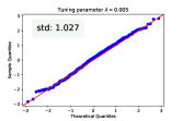
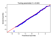
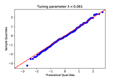
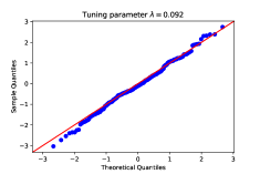
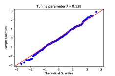
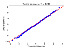
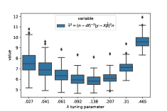
For directions such that does not hold, we expect a variance spike, i.e., an extra additive term in the variance estimate equal to in and to in . The confidence interval (3.31) that does not take into account this variance spike is expected to be too narrow and to suffer from undercoverage for directions with large . The wider confidence interval (3.32) is expected to repair this, although for directions such that does not hold the current theory does not prove whether the asymptotic distribution is normal. The theoretical evidence that the variance spike occurs is grounded in the relative asymptotic unbiasedness of in (3.23) and of in (3.25), combined with the negative result for the simpler variance estimate via Theorem 3.9 as discussed above. Figure 1 illustrates the variance spike on simulations for the Lasso and direction proportional to the first canonical basis vector.
| 0.005 | 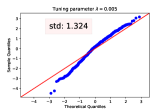 |
 |
3.23 0.45 | 0.32 0.11 |
| 0.01 | 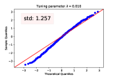 |
 |
2.62 0.41 | 0.40 0.12 |
| 0.05 | 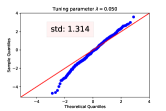 |
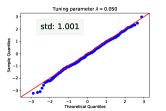 |
4.39 0.86 | 1.81 0.39 |
| 0.1 | 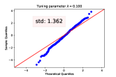 |
 |
11.70 2.40 | 5.6 1.14 |
The second term in the variance estimates (3.22) and (3.24) is necessary for certain for the estimate which corresponds to (1.2) with penalty and for . For , and ,
| (3.34) |
By the CLT, the numerator of the rightmost quantity converges to and in the denominator, by the weak law of large numbers, so that (3.34) converges in law to by Slutsky’s theorem. On the other hand, if the variance estimate is used instead of in the denominator, the CLT still holds but the asymptotic variance is .
3.8 Relaxing strong convexity when
The previous theorems are valid under Assumption 3.1: Either and is an arbitrary convex function, or and is required to be strongly convex with parameter . If and the penalty is not strongly convex, the techniques of the present paper still provide asymptotic normality results under additional assumptions as shown in the following result.
Consider either the Lasso
| (3.35) |
for some or the group Lasso norm and group Lasso defined as
| (3.36) |
where is a partition of into non-overlapping groups and are tuning parameters. If each is a singleton and for all , then (3.36) reduces to the Lasso (3.35).
Theorem 3.10.
Let be constants independent of . Consider a sequence of regression problems with and invertible . Assume that the group Lasso estimator in (3.36) satisfies
| (3.37) |
If is such that and for the in (3.26) then
| (3.38) |
Furthermore, for any with and in (3.28), the relative volume bound given after (3.28) holds, and the asymptotic normality (3.38) holds uniformly over all and uniformly over at least canonical directions in the sense that has cardinality .
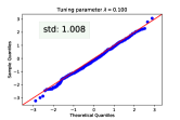
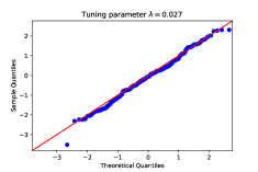
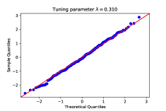
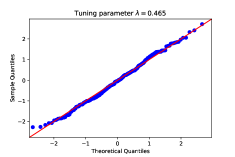
Theorem 3.10 is proved in Appendix B. The strong convexity requirement in Assumption 3.1 is relaxed and replaced by assuming the high-probability bound on the number of non-zero coordinates. Surprisingly no conditions are required on the true regression vector or on the tuning parameters, although these quantities affect whether is satisfied. Figure 2 illustrates Theorem 3.10 on simulated data.
 |
 |
 |
 |
 |
 |
 |
 |
 |
Comparison with existing works on the Lasso
The Lasso is largely the most studied initial estimator in previous literature on de-biasing and asymptotic normality, so it provides a level playing field to compare our method with existing results. In the approximate message passing (AMP) literature which includes most existing works in the regime, e.g. [20, 18, 24] or more recently [38, 29, 39, 36], it is assumed that and that the empirical distribution converges in distribution and in the second moment to some “prior” G as . Assume these conditions and consider the -th component of in (3.18) for , that is,
Then, the Lasso has the interpretation as its soft thresholded de-biased version,
and the main thrust of the AMP theory is that the joint empirical distribution of the de-biased errors and the true coefficients,
converges in distribution and the second moment to the limit with independent and components, where is characterized by a system of non-linear equations with 2 or 3 unknowns. These non-linear equations depend on the loss (here, the loss), the penalty (here, the -norm), the distribution of the noise, as well as the prior distribution that governs the empirical distribution of the coefficients of . We note that these works typically assume that has entries, so that their coefficient vector is equivalent to our . For instance, [29] characterizes the limit of the empirical distribution of in terms of two parameters, , that are defined as solutions of the non-linear equations in [29, Proposition 3.1]; see also [15, Proposition 4.3] for similar results applicable to permutation-invariant penalty. This approach presents some drawbacks: For instance it requires the convergence of the empirical distribution to a limit (which can be viewed as a prior), it yields the limiting distribution for the joint empirical distribution of the estimation errors and the unknown coefficients but not for a fixed coordinate.
The above Theorem 3.10 for the Lasso differs from this previous literature in major ways. First, it provides a limiting distribution for the de-biased version of for a single, fixed direction : Theorem 3.10 does not involve the empirical distributions of , or its de-biased version. This contrasts with previous literature on the regime where the confidence interval guarantee holds on average over the coefficients [20, 18, 24, 36]. This improvement is important in practice: if the practitioner is interested in the effect of a specific effect , it is important to construct confidence intervals with strict type I error control for , as opposed to a controlled type I error that only holds on average over all coefficients. Another feature of the results in this paper is that there is no need to assume a prior on the coefficients of in the limit.
Surprisingly, Theorems 3.6, 3.7 and 3.10 and their proofs completely bypass solving the non-linear equations that appear in the aforementioned works as the nonlinearity is directly treated here with the the normal approximation in Theorem 2.2. Moreover, Theorems 3.6, 3.7 and 3.10 handle correlations in with a direct approach, while it is still unclear whether the non-linear equations approach from previous works can be extended to .
4 Examples
We now present three penalty functions for which closed-form expressions for and are available. In this section, when computing gradients with respect to in order to find closed-form expressions for in (3.9), we consider fixed as in (3.7). Explicitly, is uniquely defined as
| (4.1) |
where and . When computing gradients with respect to in order to find closed-form expressions for in (3.3), we view as a function of and if is differentiable at for a fixed then
| (4.2) |
where is the Jacobian. Once the Jacobian is computed, in (3.3) is given by . We use the Jacobian notation when computing the derivatives with respect to to avoid confusion with the gradient in (4.1).
4.1 Twice continuously differentiable penalty
The simplest example for which closed-form expressions for can be obtained is that of twice continuously differentiable and strongly convex penalty . If is strongly convex, Lemma 5.1 proves that the Fréchet derivative of with respect to exist for almost every by Rademacher’s theorem. At a point where the derivative exist, we obtain a closed form expression for the gradient (3.9) as follows. The KKT conditions of the optimization problem (3.1) read Differentiation with respect to for a fixed as in (4.1) gives
By the product rule, this provides the derivative of , namely
| (4.3) |
Regarding involving differentiation with respect to , the Lipschitz condition of the map for strongly convex follows from (5.22) in the proof of Proposition 5.3. Hence the Jacobian in (4.2) exists almost everywhere, and differentiation of the KKT conditions for fixed gives so that
Identity (4.3) combined with this expression for provides (3.9) with
4.2 Lasso
Consider the Lasso in (3.35). For with continuous distribution such as Gaussian under consideration here, almost surely is unique and
| (4.4) |
for the Lasso as in [44, 40] and [5, Proposition 3.9], so that the Jacobian of the mapping with respect to and can be computed directly by differentiating the KKT condition as in [40, 5, 6]. The following proposition provides closed-form expressions for the gradients for the Lasso estimator which are valid almost surely and require no assumption on the sparsity of or the penalty level.
Proposition 4.1.
Proof of Proposition 4.1.
Proposition 3.9 in [5] proves, for almost every , uniqueness of and (4.4). Let be a point at which (4.4) holds. It follows from (4.4) and the Holder continuity of established after (5.2) that for almost every there is an open neighborhood in n×(p+1) in which , and are constants, so that is locally equal to with the linear penalty . In this neighborhood has the analytic expression
Differentiating the above immediately yields the formulas for , and . For , differentiating both sides of yields
due to . Finally, the formula for follows from and simple algebra. ∎
4.3 Group Lasso
Consider a partition of and the group Lasso estimator in (3.36). Let be the set of active groups and the union of all active groups. Define the block diagonal matrix by
| (4.5) |
The following proposition provides closed-form expressions for the gradients for the Group Lasso estimator and related quantities and in terms of and . Its proof is given in Appendix C. Note that the formula for was known [41].
Proposition 4.2.
The following holds for for almost every . The set of active groups is the same for all minimizers of (3.36) at and for all in a sufficiently small neighborhood of . If additionally is invertible where then the map is Lipschitz in a sufficiently small neighborhood of . In this neighborhood we have
and (3.9) holds with .
5 Proof of the main results in Section 3
In order to prove Theorems 3.6 and 3.7, we apply the bound on the normal approximation in Theorem 2.2. We recall here some notation used throughout the proof. Let be the estimator (3.1), the gradient of as in (1.8), with , and as defined in (1.15),
| (5.1) |
Vector is given by Lemma 3.1. The oracle and its associated noiseless prediction risk are given by (3.26). Throughout, denotes the conditional expectation given and the conditional variance given .
5.1 Lipschitzness of regularized least-squares and existence of
By Rademacher’s theorem, a Lipschitz function for some open set is Fréchet differentiable almost everywhere in . The following lemma is the device that verifies the Lipschitz condition for the mappings and in certain open set , and consequently differentiability almost everywhere in .
Lemma 5.1.
Let , and be two design matrices of size , and and two noise vectors in n. Let be convex such that minimizers
exist. Let , , , . Let also where is the subdifferential at given by the optimality condition of the above optimization problem and similarly for , with by the monotonicity of the subdifferential. Then
| (5.2) | |||||
| (5.3) |
If is coercive (i.e., as ) then the map is Holder continuous with coefficient on every compact. We also have
| (5.4) | |||
| (5.5) | |||
If either is strongly convex or if there exists a constant and a bounded neighborhood of such that for all then the map is Lipschitz in .
Proof of Lemma 5.1.
By optimality of , . If is coercive, this implies that for every compact , and are bounded by a constant depending only on if . In this case, (5.2) implies that for some other constant depending on only. This implies Holder continuity of with Holder coefficient on every compact.
For (5.4) and (5.5), the KKT conditions for yield
Summing the above and its counterpart yields the equality (5.4). Writing and similarly , inequality (5.5) follows. To prove the Lipschitz condition in , we note that for a fixed value of , the right hand side of (5.5) is linear in while the left-hand side is quadratic in thanks to either strong convexity of or the assumption on . This implies that is bounded uniformly for all in . Since are all bounded in , (5.5) divided by provides the desired Lipschitz property. ∎
See 3.1
Proof of Lemma 3.1.
Under Assumption 3.1, Lemma 5.1 implies that the map is Lipschitz in an open neighborhood of almost every point, and thus and are defined as Fréchet derivatives almost surely in (3.3) and (3.6) respectively. To prove (3.9), i.e. that the range of is the linear span of , we study the directional derivative in a direction . For two pairs and with and , consider the solutions and defined in Lemma 5.1 and with . When the map is Fréchet differentiable at ,
| (5.6) |
by the chain rule and the linearity of the Fréchet derivative, noting that . For this specific choice of we have
| (5.7) |
It follows that the second term in the first line of (5.2) is zero, so that (5.2) gives
due to . Consequently when . This and (5.6) give (3.9). Moreover, for , for , so that (3.10) is an upper bound for in the case of where
by the previous display. For , the above inequality gives using . For ,
with being the smallest eigenvalue of . Hence, (3.10) holds in either cases. ∎
5.2 Loss equivalence to oracle estimators
To apply Theorem 2.2 with respect to to in (5.1), we will need to control expectations involving , , and . To this end, define the random variables and by
| (5.8) |
with and the and in (3.26), and
| (5.9) |
We note that the three random vectors and have distribution, so that is of the form where each has the distribution. Thus by Proposition A.1 and properties of the distribution,
| (5.10) |
It follows from (1.17), Lemma 5.2 below and (3.10) that almost surely
| (5.11) | |||
| (5.12) |
for the in Lemma 3.1. The moment inequalities in (5.10) and the almost sure bounds (5.11)-(5.12) allow us to control expectations involving , , and throughout the proofs. The following lemma provides the first inequality in (5.11).
Lemma 5.2 (Deterministic lemma).
Proof of Lemma 5.2.
The KKT conditions for , i.e., , yield
Similarly, the KKT conditions for yield
| (5.16) |
Summing the two above displays yields
| (5.17) | |||||
| (5.18) |
For , by the triangle inequality
| (5.19) |
provides a lower bound on the left-hand side of (5.17) so that
| (5.20) | |||||
| (5.21) |
due to in the second case. This gives (5.15). For by (5.17), (5.19) and (5.20) we have
and for we have and thus (5.15) holds. ∎
5.3 Existence and properties of and
Proposition 5.3.
Let be any fixed design matrix, and . Then, the following statements hold.
-
(i)
for all , i.e., is 1-Lipschitz. Its gradient exists almost everywhere by Rademacher’s theorem, that is, for almost every there exists with such that .
-
(ii)
For almost every , matrix is symmetric with eigenvalues in . Consequently, with as degrees of freedom, .
Proof.
A proof of (i) is given in [4]. For completeness, the argument is the following: by (5.4) with , and we have
| (5.22) |
Using by monotonicity of the subdifferential and the Cauchy-Schwarz inequality yields the desired Lipschitz property. For (ii), define
The function is convex in as a supremum of affine functions, and is a subgradient of at . Alexandrov’s theorem as stated in [31, Theorem D.2.1] states that any convex is twice differentiable at for almost every in the following sense: is Fréchet differentiable at with gradient and there exists a symmetric positive semi-definite matrix such that for every there exists such that for all ,
By (i) and the definition of , for almost every it holds that . Combining these two results and taking , we get that for almost every . ∎
Lemma 5.4.
Let Assumption 3.1 be fulfilled with . Then there exists an event independent of such that
where depends on only.
Proof of Lemma 5.4.
If , the choice works with probability one because and .
If then we have in Assumption 3.1. Let . By [17, Theorem II.13], due to with . Next, we hold fixed and study the derivatives of with respect to . Let be as in Proposition 5.3. Let be the projection onto so that . Let be such that , or equivalently . By (5.22) and (3.2),
On , . Combined with the above display, this implies . With and by definition of we have for , hence . Since , by Cauchy’s interlacing theorem has at least eigenvalues no smaller than . Finally, since is symmetric with eigenvalues in by Proposition 5.3,
with thanks to . ∎
5.4 Lower bound on
The following lemmas are useful to bound from below the denominator in (3.27).
Lemma 5.5.
Proof of Lemma 5.5.
By (3.9) combined with (3.10), (5.12) and (5.10),
| (5.25) |
Similarly, by definition of in (3.21), . Using (5.11)-(5.12) we have and
| (5.26) | |||||
thanks to in (3.9), and for the first inequality, by Proposition 5.3 and (5.25) for the second inequality, and (5.11)-(5.10) for the third inequality. This provides . Next, (5.23) holds due the bound (5.25) and the relationship in (3.11) between , and the integrand in left-hand side of (5.23). Then (5.24) follows from (5.23) and by Lemma 5.4. ∎
Lemma 5.6.
Proof of Lemma 5.6.
By the triangle inequality and definitions of ,
| (5.33) | ||||
| (5.34) | ||||
where the last line follows from the weighted sum and using for the last two terms. By the KKT conditions of and ,
Summing these equalities and using the monotonicity of the subdifferential yields
| (5.35) | |||||
| (5.36) |
Combining (5.35) multiplied by with the line after (5.34) gives
using the Cauchy-Schwarz inequality and for the last inequality. Using for the right-hand side with completes the proof of (5.28). The second inequality, (5.29), then follows from (3.9), (3.21) and
which implies . ∎
Lemma 5.7.
Define where are defined in Lemma 5.6. Under Assumption 3.1 we have .
Proof of Lemma 5.7.
We bound each of separately. We have by (5.12) so that by virtue of (5.10). For we have . By the Second Order Stein formula (Proposition 2.1) with respect to conditionally on ,
where we used from Proposition 5.3 and (5.12) for the inequality. Thanks to (5.10), this shows that . Similarly for in (5.29), hence by (5.12) and (5.10). For we have for so that by (5.23). ∎
5.5 Event
5.6 Proofs of Lemmas 3.2, 3.4 and 3.5 and Theorem 3.9
See 3.2
See 3.4
Proof of Lemma 3.4.
Let be as in (5.37). The first inequality in (3.23) follows from the triangle inequality. By (5.40) we have . With in (3.21)-(3.22) and in (3.9),
Using from Proposition 5.3 and (5.11)-(5.12) we find by the Cauchy-Schwarz inequality . The proof of (3.23) is complete by virtue Holder’s inequality and the moment bounds (5.10). ∎
See 3.5
Proof of Lemma 3.5.
By the triangle inequality for the Euclidean norm in 2,
| (5.41) |
Let be as in (5.37). Using , the lower bound (5.39) and by Proposition 5.3,
so that and (5.24) completes the proof for the first term in the maximum in (3.25). For the second term in the maximum, by the triangle inequality for the norm , we have . The proof is completed by using again (5.41), the lower bound (5.40) on in and the same argument as for the first term in the maximum. ∎
See 3.9
Proof of Theorem 3.9.
(v) (iv) is due to in by Lemma 5.4 and Proposition 5.3 combined with (3.20).
(iv) (vi) follows from in .
(vi) (vii) is proved in Lemma 3.5.
(iii) (i), (iii) (vi) and (iii) (vii), are shown in the proof of Theorem 3.6.
(iii) was shown in the proof of Theorem 3.6, and implies and so that (iii) (ii) holds.
5.7 Proofs of Theorem 3.3 and asymptotic normality results
See 3.3
Proof of Theorem 3.3.
See 3.6
Proof of Theorem 3.6.
Let be as in (5.37). Let be the quantity in (3.27), omitting the dependence in as it is clear from context. Since by definition, . In , (5.40) provides a lower bound on the denominator of so that . By (5.26) and the bound (5.38) on , we obtain
| (5.42) |
Furthermore, is bounded in thanks to by (5.11) and (5.10). Since a sequence of random variables uniformly bounded in is uniformly integrable, the assumption implies and thus . This completes the proof that and that by Theorem 2.2. Next, by (3.19), also holds. It remains to prove for all four possible choices for . By (2.7), implies , while
| (5.43) |
Proposition 5.3 provides so that the numerator converges to 0 in probability thanks to assumption . The denominator is bounded from below by in by (5.39) and . This proves and follows by Lemma 3.5. Slutsky’s theorem completes the proof as for all four possible choices for . As is continuous, convergence in Kolmogorov distance is equivalent to convergence in distribution. ∎
See 3.7
Proof of Theorem 3.7.
We construct a subset of the sphere such that uniformly over all . Let be uniformly distributed on the unit Euclidean sphere , independently of , and denote by its probability measure. The vector is subgaussian in p [43, Theorem 3.4.6], in the sense that for any non-zero vector , for some absolute constant . By Jensen’s inequality and Fubini’s Theorem,
Hence by Markov’s inequality, for any positive , . Setting , we obtain that the subset defined by (3.28) has relative volume at least , and for all ,
| (5.44) |
Furthermore, the set has cardinality at least due to
To show that , thanks to (5.42) it is enough to prove that uniformly over . By the Cauchy-Schwarz inequality,
for any thanks to (5.44), while by (5.11) and (5.10). This implies and hold.
By Theorem 2.2 this shows that uniformly over . Since the bounds (3.17), (5.43) are all uniform over all with , Slutsky’s theorem implies , and uniformly over for all four possible choices for , and convergence in Kolmogorov distance follows from convergence in distribution. ∎
See 3.8
Proof of Theorem 3.8.
The first statement of the theorem follows from Lemma 5.5. Finally, if is a norm then the KKT conditions of , since for a norm . ∎
Appendix A Integrability of when
In our regression model with Gaussian covariates, the matrix has iid entries, and the inverse of its smallest singular value enjoys the following integrability property as with .
Proposition A.1.
Let and let be a matrix with rows, columns and iid entries. Then is a Wishart matrix and if with we have for any constant not growing with ,
Proof.
Throughout the proof, is an implicit function of ; we omit the subscript for brevity. Since almost surely (cf. [32]), it is enough to show that the sequence of random variables is uniformly integrable for some , i.e., that as For uniform integrability, we use the following argument from [19, Section 5]. The matrix is a Wishart matrix and the density of satisfies for ,
cf. [19, Section 5]. The density of that we are interested in, is given by for . Hence if ,
The mode of the integrand over is . Thanks to , there exists some such that for all ,
| (A.1) |
is smaller than the mode and the integral above is bounded by . Let denote the bracket of the previous display. Then using Stirling’s formula , we have for some constants possibly depending on
because the main terms (coming from in Stirling’s formula) cancel each other. Then for any ,
| (A.2) | |||||
| (A.3) |
For , (A.1) holds and if we have
which converges to as . This shows uniform integrability of the sequence and proves the claim. ∎
Appendix B Proof: without strong convexity
Lemma B.1.
Let and assume that . Then for any ,
for some constant depending only on .
Proof.
If is a subspace of dimension and then by (A.2) with , and large enough,
for constant thanks to . Applying this bound to the subspace for with and using the union bound,
using with and . Since , choosing the right-hand side of the previous display is bounded from above by . This value of provides . ∎
See 3.10
Proof of Theorem 3.10.
As in the rest of the paper, and we wish to apply Theorem 2.2 to conditionally on . Instead of applying Theorem 2.2 to , and in order to avoid certain events of small probability where the sparse eigenvalues of are not well behaved, we will apply it to a different function. Consider in (5.8) and the events
where is the constant from Lemma B.1. Finally, let be the event (C.1) that the KKT conditions of hold strictly, and set
We have by (3.37) and standard concentration bounds for random variables [26, Lemma 1] give . Lemma B.1 and [17, Theorem II.13] provide and (C.1) gives . These bounds imply by the union bound.
As the only randomness of the problem comes from , we may choose the underlying probability space as , so that are subsets of . We next prove that is open as a subset of . Indeed, because the KKT conditions are strict in , is a disjoint union of sets of the form
| (B.1) |
over all possible active groups . The sets are open as the inequalities are strict. In the function is locally Lipschitz by Lemma 5.1, hence continuous. By continuity, the preimage of the open set by the function , is open by continuity, and the preimage of the open set by the function , is also open, again by continuity. This shows that the set (B.1) is open for any fixed so that is open as the union of sets of the form (B.1) over all satisfying . This proves that is open.
For in Lemma 5.2, (5.13) is satisfied so that (5.15)-(5.15) hold. In , we thus have and . Furthermore in thanks to and the explicit expression for in Proposition 4.2. In summary we have in
| (B.2) |
which replace (5.11)-(5.12) in the present context. By the deterministic inequality (5.33), in we have since is rank at most with operator norm at most one, so that
| (B.3) |
Let both in , let , and let be as in Lemma 5.1. Thanks to event and the fact that and similarly for we have . Thus by (5.4),
Summing this inequality with the first line in (5.2) we find
| (B.4) | |||||
| (B.6) | |||||
Thanks to the bounds in (B.2), this implies if , where .
For a given , we define . In , the function is -Lipschitz. By Kirszbraun’s theorem, there exists a function that is an extension of , i.e., for , and such that is -Lipschitz in the whole n. Note that both function and implicitly depend on . Since is open, is also open, and thus conditionally on ,
| (B.7) |
(Without the openness of established above, equality of the gradients would be unclear).
Since is such that in , by (B.3)
| (B.8) | |||||
| (B.9) |
Taking conditional expectations and multiplying both sides by we find
due to for the first term and for the second. Using and ,
where we used that in since is -Lipschitz. We now prove that the three terms on the right-hand side of converge to 0. For the third term, and as has probability approaching one. For the first term, since is -Lipschitz, almost surely so that the sequence of random variables is uniformly integrable. Thanks to uniform integrability, if we can prove then holds. We use that by (B.7), and that in the gradients of with respect to are given in Proposition 4.2 so that by (B.2)
which converges to 0 in probability thanks to assumption . Thanks to uniform integrability, this proves . It remains to show . By definition of in (5.31), thanks to and (B.2) we have . For in (5.30), let be the convex projection onto the Euclidean ball of radius , then in by (B.2) so that
| (B.10) | |||||
| (B.11) | |||||
| (B.12) |
by applying Proposition 2.1 to the function which is 1-Lipschitz as the composition of two 1-Lipschitz functions (cf. Proposition 5.3(i)). For in (5.32), let by as in Lemma 5.6 and set , and note that for . Let also be the from Proposition 4.2 for . As above for , for a fixed the function is -Lipschitz in by (B.4) for the value of given after (B.4). Furthermore in . By Kirszbraun’s theorem, there exists an extension implicitly depending on such that in and by composing the extension given by Kirszbraun’s theorem by the convex projection onto the Euclidean ball of radius . By Proposition 2.1 with respect to conditionally on
For the value of given after (B.4) and using the bound (B.2) to control in , this gives .
This proves . Consequently satisfies by (2.9). Since is equal to on the event because is an extension of , we have so that as well. The conclusion (3.38) is obtained by controlling the term by which is bounded as in (B.2) in .
It remains to show that (3.38) holds uniformly over all and to derive the properties of . The proof of the relative volume bound on and the lower bound on the cardinality of is the same as in the proof of Theorem 3.7 given around (5.44), and for inequality (5.44) holds. For such , by (B.2) for the first inequality and (5.44) for the second. ∎
Appendix C Strict KKT conditions with probability one for the group Lasso
Lemma C.1.
Consider a design matrix and a response vector for which the joint distribution of admits a density with respect to the Lebesgue measure. Consider a partition of into groups and any minimizer
for some deterministic . There exists an open set such that and the KKT conditions are strict in in the sense that
| (C.1) |
Finally, is constant in a small neighborhood of any point in .
Proof of Lemma C.1.
Consider a fixed and its complementary set , and consider the Group-Lasso estimator with the additional constraint for every . Now consider a group . Since the joint distribution of has a density with respect to the Lebesgue measure, the conditional distribution of given also admits a density with respect to the Lebesgue measure. Conditionally on , two cases may appear:
-
(i)
If , the KKT condition for group hold strictly since .
-
(ii)
If , the distribution of given and the distribution of given both have a density with respect to the Lebesgue measure. The sphere of radius has measure 0 for any continuous distribution, hence
Finally, the unconditional probability is also one. Let . Then as a finite intersection of events of probability one and (C.1) holds. The set is open as a finite intersection of open sets, since is open by continuity of by the claim following (5.2).
Next, to show that is constant in a neighborhood of every point in , set for all . We have and the set is open by continuity of , which follows from the continuity of by the claim following (5.2). For any , there exists some with . Let . By continuity of thanks to the claim following (5.2), there exists a neighborhood of with such that for all , for and for . Since , implies so that that in . ∎
See 4.2
Proof of Proposition 4.2.
By Lemma C.1, and are constant in a sufficiently small neighborhood of almost every . The additional assumption that is invertible provides that is invertible by continuity of the smallest eigenvalue in a small enough compact neighborhood of , and in this neighborhood is Lipschitz by the sentence following (5.5) and thus almost everywhere differentiable by Rademacher’s theorem. The formulae for , and involving the matrix in (4.5) are then obtained by differentiating the KKT conditions restricted to in this neighborhood, that is, for all . ∎
Appendix D Proof of Theorem 2.3
Proof of Theorem 2.3.
References
- Bayati and Montanari [2012] Mohsen Bayati and Andrea Montanari. The lasso risk for gaussian matrices. IEEE Transactions on Information Theory, 58(4):1997–2017, 2012.
- Bellec [2018a] Pierre C Bellec. The noise barrier and the large signal bias of the lasso and other convex estimators. arXiv:1804.01230, 2018a. URL https://arxiv.org/pdf/1804.01230.pdf.
- Bellec [2018b] Pierre C Bellec. The noise barrier and the large signal bias of the lasso and other convex estimators. arXiv preprint arXiv:1804.01230, 2018b.
- Bellec and Tsybakov [2017] Pierre C Bellec and Alexandre B Tsybakov. Bounds on the prediction error of penalized least squares estimators with convex penalty. In Vladimir Panov, editor, Modern Problems of Stochastic Analysis and Statistics, Selected Contributions In Honor of Valentin Konakov. Springer, 2017. URL https://arxiv.org/pdf/1609.06675.pdf.
- Bellec and Zhang [2018] Pierre C Bellec and Cun-Hui Zhang. Second order stein: Sure for sure and other applications in high-dimensional inference. arXiv preprint arXiv:1811.04121, 2018.
- Bellec and Zhang [2019] Pierre C Bellec and Cun-Hui Zhang. De-biasing the lasso with degrees-of-freedom adjustment. preprint, 2019.
- Bellec et al. [2018] Pierre C. Bellec, Guillaume Lecué, and Alexandre B. Tsybakov. Slope meets lasso: Improved oracle bounds and optimality. Ann. Statist., 46(6B):3603–3642, 2018. ISSN 0090-5364. URL https://arxiv.org/pdf/1605.08651.pdf.
- Belloni et al. [2014] Alexandre Belloni, Victor Chernozhukov, and Christian Hansen. High-dimensional methods and inference on structural and treatment effects. Journal of Economic Perspectives, 28(2):29–50, 2014.
- Bickel et al. [1993] Peter J Bickel, Chris AJ Klaassen, Peter J Bickel, Y Ritov, J Klaassen, Jon A Wellner, and YA’Acov Ritov. Efficient and adaptive estimation for semiparametric models. Johns Hopkins University Press Baltimore, 1993.
- Bickel et al. [2009] Peter J. Bickel, Yaacov Ritov, and Alexandre B. Tsybakov. Simultaneous analysis of lasso and dantzig selector. Ann. Statist., 37(4):1705–1732, 08 2009. 10.1214/08-AOS620. URL http://dx.doi.org/10.1214/08-AOS620.
- Blumensath and Davies [2009] Thomas Blumensath and Mike E Davies. Iterative hard thresholding for compressed sensing. Applied and computational harmonic analysis, 27(3):265–274, 2009.
- Bogachev [1998] Vladimir Igorevich Bogachev. Gaussian measures. Number 62. American Mathematical Soc., 1998.
- Bu et al. [2019] Zhiqi Bu, Jason Klusowski, Cynthia Rush, and Weijie Su. Algorithmic analysis and statistical estimation of slope via approximate message passing. In Advances in Neural Information Processing Systems, pages 9361–9371, 2019.
- Cai and Guo [2017] T Tony Cai and Zijian Guo. Confidence intervals for high-dimensional linear regression: Minimax rates and adaptivity. The Annals of statistics, 45(2):615–646, 2017.
- Celentano and Montanari [2019] Michael Celentano and Andrea Montanari. Fundamental barriers to high-dimensional regression with convex penalties. arXiv preprint arXiv:1903.10603, 2019.
- Chatterjee [2009] Sourav Chatterjee. Fluctuations of eigenvalues and second order poincaré inequalities. Probability Theory and Related Fields, 143(1-2):1–40, 2009.
- Davidson and Szarek [2001] Kenneth R Davidson and Stanislaw J Szarek. Local operator theory, random matrices and banach spaces. Handbook of the geometry of Banach spaces, 1(317-366):131, 2001.
- Donoho and Montanari [2016] David Donoho and Andrea Montanari. High dimensional robust m-estimation: Asymptotic variance via approximate message passing. Probability Theory and Related Fields, 166(3-4):935–969, 2016.
- Edelman [1988] Alan Edelman. Eigenvalues and condition numbers of random matrices. SIAM Journal on Matrix Analysis and Applications, 9(4):543–560, 1988.
- El Karoui et al. [2013] Noureddine El Karoui, Derek Bean, Peter J Bickel, Chinghway Lim, and Bin Yu. On robust regression with high-dimensional predictors. Proceedings of the National Academy of Sciences, 110(36):14557–14562, 2013.
- Fan and Li [2001] Jianqing Fan and Runze Li. Variable selection via nonconcave penalized likelihood and its oracle properties. Journal of the American statistical Association, 96(456):1348–1360, 2001.
- Feng and Zhang [2019] Long Feng and Cun-Hui Zhang. Sorted concave penalized regression. Annals of Statistics, 47(6):3069–3098, 2019.
- Javanmard and Montanari [2014a] Adel Javanmard and Andrea Montanari. Confidence intervals and hypothesis testing for high-dimensional regression. The Journal of Machine Learning Research, 15(1):2869–2909, 2014a.
- Javanmard and Montanari [2014b] Adel Javanmard and Andrea Montanari. Hypothesis testing in high-dimensional regression under the gaussian random design model: Asymptotic theory. IEEE Transactions on Information Theory, 60(10):6522–6554, 2014b.
- Javanmard and Montanari [2018] Adel Javanmard and Andrea Montanari. Debiasing the lasso: Optimal sample size for gaussian designs. The Annals of Statistics, 46(6A):2593–2622, 2018.
- Laurent and Massart [2000] B. Laurent and P. Massart. Adaptive estimation of a quadratic functional by model selection. Ann. Statist., 28(5):1302–1338, 10 2000. 10.1214/aos/1015957395. URL http://dx.doi.org/10.1214/aos/1015957395.
- Lecué and Mendelson [2018] Guillaume Lecué and Shahar Mendelson. Regularization and the small-ball method i: Sparse recovery. Ann. Statist., 46(2):611–641, 04 2018. 10.1214/17-AOS1562. URL https://doi.org/10.1214/17-AOS1562.
- Lei et al. [2018] Lihua Lei, Peter J Bickel, and Noureddine El Karoui. Asymptotics for high dimensional regression m-estimates: fixed design results. Probability Theory and Related Fields, 172(3-4):983–1079, 2018.
- Miolane and Montanari [2018] Léo Miolane and Andrea Montanari. The distribution of the lasso: Uniform control over sparse balls and adaptive parameter tuning. arXiv preprint arXiv:1811.01212, 2018.
- Ndaoud [2020] Mohamed Ndaoud. Scaled minimax optimality in high-dimensional linear regression: A non-convex algorithmic regularization approach. arXiv preprint arXiv:2008.12236, 2020.
- Niculescu and Persson [2006] Constantin Niculescu and Lars-Erik Persson. Convex functions and their applications. Springer, 2006.
- Silverstein [1985] Jack W Silverstein. The smallest eigenvalue of a large dimensional wishart matrix. The Annals of Probability, 13(4):1364–1368, 1985.
- Stein [1981] Charles M Stein. Estimation of the mean of a multivariate normal distribution. The annals of Statistics, pages 1135–1151, 1981.
- Sun and Zhang [2012] Tingni Sun and Cun-Hui Zhang. Scaled sparse linear regression. Biometrika, 99(4):879–898, 2012.
- Sun and Zhang [2013] Tingni Sun and Cun-Hui Zhang. Sparse matrix inversion with scaled lasso. The Journal of Machine Learning Research, 14(1):3385–3418, 2013.
- Sur and Candès [2018] Pragya Sur and Emmanuel J Candès. A modern maximum-likelihood theory for high-dimensional logistic regression. arXiv preprint arXiv:1803.06964, 2018.
- Talagrand [2010] Michel Talagrand. Mean field models for spin glasses: Volume I: Basic examples, volume 54. Springer, 2010.
- Thrampoulidis et al. [2015] Christos Thrampoulidis, Ehsan Abbasi, and Babak Hassibi. Lasso with non-linear measurements is equivalent to one with linear measurements. In Advances in Neural Information Processing Systems, pages 3420–3428, 2015.
- Thrampoulidis et al. [2018] Christos Thrampoulidis, Ehsan Abbasi, and Babak Hassibi. Precise error analysis of regularized -estimators in high dimensions. IEEE Transactions on Information Theory, 64(8):5592–5628, 2018.
- Tibshirani [2013] Ryan J Tibshirani. The lasso problem and uniqueness. Electronic Journal of Statistics, 7:1456–1490, 2013.
- Vaiter et al. [2012] Samuel Vaiter, Charles Deledalle, Gabriel Peyré, Jalal Fadili, and Charles Dossal. The degrees of freedom of the group lasso. arXiv preprint arXiv:1205.1481, 2012.
- Van de Geer et al. [2014] Sara Van de Geer, Peter Bühlmann, Ya’acov Ritov, and Ruben Dezeure. On asymptotically optimal confidence regions and tests for high-dimensional models. The Annals of Statistics, 42(3):1166–1202, 2014.
- Vershynin [2018] Roman Vershynin. High-dimensional probability: An introduction with applications in data science, volume 47. Cambridge University Press, 2018.
- Zhang [2010] Cun-Hui Zhang. Nearly unbiased variable selection under minimax concave penalty. The Annals of statistics, 38(2):894–942, 2010.
- Zhang [2011] Cun-Hui Zhang. Statistical inference for high-dimensional data. Mathematisches Forschungsinstitut Oberwolfach: Very High Dimensional Semiparametric Models, Report, (48):28–31, 2011.
- Zhang and Huang [2008] Cun-Hui Zhang and Jian Huang. The sparsity and bias of the lasso selection in high-dimensional linear regression. Ann. Statist., 36(4):1567–1594, 08 2008. URL https://doi.org/10.1214/07-AOS520.
- Zhang and Zhang [2014] Cun-Hui Zhang and Stephanie S Zhang. Confidence intervals for low dimensional parameters in high dimensional linear models. Journal of the Royal Statistical Society: Series B (Statistical Methodology), 76(1):217–242, 2014.