Abstract

We consider the optimization problem associated with fitting two-layer ReLU networks with respect to the squared loss, where labels are assumed to be generated by a target network. Focusing first on standard Gaussian inputs, we show that the structure of spurious local minima detected by stochastic gradient descent (SGD) is, in a well-defined sense, the least loss of symmetry with respect to the target weights. A closer look at the analysis indicates that this principle of least symmetry breaking may apply to a broader range of settings. Motivated by this, we conduct a series of experiments which corroborate this hypothesis for different classes of non-isotropic non-product distributions, smooth activation functions and networks with a few layers.

1 Introduction

The great empirical success of artificial neural networks over the past few years has challenged the very foundations of our understanding of statistical learning processes. Although fitting generic high-dimensional nonconvex models is typicality a lost cause, multilayered ReLU networks achieve state-of-the-art performance in many machine learning tasks, while being trained using numerical solvers as simple as stochastic first-order methods. Given this perplexing state of affairs, a large body of recent works has focused on various two-layers networks as a more manageable means of investigating some of the complexity exhibited by deep models. One such major line of research has been concerned with exploring the set of assumptions under which the loss surface of Gaussian inputs qualifies convergence of various local search methods (e.g., [12, 17, 26, 19, 40, 22, 37]). Recently, Safran & Shamir [33] considered the well-studied two-layers ReLU network ${\bm{x}}\mapsto\bm{1}^{\top}_{k}\phi({\bm{W}}{\bm{x}})$, where ${\bm{x}}\in\mathbb{R}^{d},{\bm{W}}\in M\left(k,d\right)$, $\phi(z)~{}\dot{=}~{}\max\{0,z\}$ and $\bm{1}_{k}$ is the $k$-dimensional vector of all ones, and proved that the expected squared loss w.r.t. a target network with identity weight matrix, i.e.,

$${\mathcal{L}}({\bm{W}})~{}\dot{=}~{}\frac{1}{2}\mathbb{E}_{{\bm{x}}\sim\mathcal{N}({\bm{0}},{\bm{I}}_{d})}\left[(\bm{1}^{\top}_{k}\phi({\bm{W}}{\bm{x}})-\bm{1}^{\top}_{d}\phi({\bm{x}}))^{2}\right],\quad{\bm{W}}\in M\left(k,d\right),$$ (1.1)

possesses a large number of spurious local minima which can cause gradient-based methods to fail.

Unlike the existence of multiple spurious local minima, the fact that ${\mathcal{L}}$ contains many global minima should come as no surprise—it is a consequence of symmetry properties of ${\mathcal{L}}$. Indeed, assuming for the moment that $k=d$, ${\mathcal{L}}$ is invariant under all transformations of the form ${\bm{W}}\mapsto{\bm{P}}_{\pi}{\bm{W}}{\bm{P}}_{\rho}^{\top},\pi,\rho\in S_{d}$, where $S_{d}$ is the symmetric group of degree $d$, and ${\bm{P}}_{\pi},{\bm{P}}_{\rho}$ are the associated permutation matrices which permute the rows and the columns of ${\bm{W}}$ respectively (see Section 4 for more details). In particular, since the identity matrix is a global minimizer, so is every permutation matrix. Permutation matrices are highly ‘symmetric’ in the sense that the group of all row and column permutations that fix a permutation matrix ${\bm{P}}$ — the isotropy group of ${\bm{P}}$ — is isomorphic to $\Delta{S_{d}}~{}\dot{=}~{}\{{\bm{W}}\mapsto{\bm{P}}_{\pi}{\bm{W}}{\bm{P}}_{\pi}^{\top}~{}|~{}\pi\in S_{d}\}$ (this is obvious for ${\bm{W}}={\bm{I}}_{d}$, since ${\bm{I}}_{d}={\bm{P}}_{\pi}{\bm{I}}_{d}{\bm{P}}_{\pi}^{\top}$ holds trivially for any $\pi\in S_{d}$). With this in mind, one may ask

How symmetric are local minima, which are not global?

In this work, we show that, perhaps surprisingly, the isotropy subgroups of spurious local minima of ${\mathcal{L}}$ are maximal (or large) in $\Delta S_{d}$, the isotropy of the global solution ${\bm{W}}={\bm{I}}_{d}$. In other words, spurious local minima exhibit the least symmetry loss w.r.t. the symmetry of the target model. This provides a natural explanation for the patterns that appear in the local minima found in [33] (see Figure 1). Next, in examining the predictive power of such a principle, we ask how does the symmetry of local minima change if $d$ is even and the target model is of reduced symmetry, say, ${\bm{W}}={\bm{I}}_{d/2}\oplus 2{\bm{I}}_{d/2}$ whose isotropy is $\Delta S_{{d}/{2}}\times\Delta S_{{d}/{2}}$? Similarly, we find that maximal isotropy subgroups correctly predict the shape of critical points detected by SGD. A more detailed analysis reveals that the invariance properties of ${\mathcal{L}}$ do not directly depend on the rotational invariance of standard Gaussian inputs. Indeed, the same structure of critical points is observed when the input is drawn uniformly at random from $[-1,1]^{d}$, suggesting that isotropy type of critical points strongly depend on the intricate interplay between the network architecture, the input distribution and the label distribution (cf. [12, 35] and references therein, for hardness results of learnability under partial sets of assumptions).

It is noteworthy that this phenomenon, in which critical points of invariant functions exhibit maximal (or large) isotropy groups, has been observed many times in various scientific fields; for example in Higgs-Landau theory, equivariant bifurcation theory and replica symmetry breaking (see, e.g.,[29, 23, 20, 14]). It appears that ReLU networks form a rather unexpected instance for this principle.

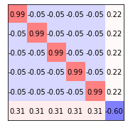
Figure 1: Top: a $6\times 6$ spurious minimum of (1.1) [33, Example 1]. Bottom: maximal isotropy $\Delta S_{5}\times\Delta S_{1}$ in $\Delta S_{6}$, the isotropy of the global solution ${\bm{I}}_{6}$ $(\alpha,\beta,\gamma,\delta,\epsilon\in\mathbb{R})$.

Our contributions (in order of appearance) can be stated as follows:

• We express the invariance properties of ReLU networks in terms of the network architecture, as well as the underlying data distribution. As a simple application, we show that the auto-balancing property introduced in [16] can be reformulated as a conservation law induced by a suitable continuous symmetry. This provides an alternative and arguably more natural derivation of this property.

• We analyze the intricate isotropy subgroup lattice of $S_{k}\times S_{d}$ and $\Delta S_{d}$, and characterize large classes of the respective maximal isotropy subgroups. Our purely theoretical analysis gives a precise description of the structure of spurious local minima detected by SGD for ReLU network (1.1). We show that this is consistent over various target weight matrices.

• We conduct a series of experiments which examine how the isotropy types of critical points depend on the joint symmetry of the target model, the underlying distribution and the network architecture. Our findings indicate that a similar phenomenon indeed applies to other related problems with, e.g., Leaky-ReLU and softplus activation functions, slightly over-specified parameterization and a few fully-connected layers. We also demonstrate some settings where this phenomenon does not occur.

The paper is organized as follows. After surveying related work below, and relevant group-theoretic background in Section 3, we present a simple derivation of the auto-balancing property based on symmetry arguments. In Section 4 we provide a detailed analysis of the invariance properties of ReLU networks and the corresponding isotropy lattice. Lastly, we present in Section 5 empirical results which examine the scope of the least (or small) symmetry breaking principle. All proofs are deferred to the appendix.

2 Related Works

Two-layer ReLU networks, the main focus of this work, have been studied under various settings which differ by their choice of, for example, activation function, underlying data distribution, number of hidden layers w.r.t. number of samples and numerical solvers ([13, 25, 36, 39, 41, 31, 18, 24]). Closer to our settings are works which consider Gaussian inputs and related obstacles for optimization methods, such as bad local minima. [40, 17, 19, 26, 37, 12, 22]. Most notably, the spurious minima addressed by [33] exhibit the very symmetry claimed in this work. Another relevant line of works have studied trainability of ReLU multilayered networks directly through the lens of symmetry. Concretely, it is shown that the rich weight-space symmetry carries important information on singularities which can significantly harm the convergence of gradient-based methods [32, 1, 38, 30, 11]. In contrast to this, symmetry here is utilized as a mean of studying the structure of critical points, rather than characterizing various regions of the loss landscape.

Symmetry breaking in nonconvex optimization

The present work has been the precursor to a rapidly growing body of work building on the phenomena of symmetry breaking first reported and studied here. In [6], path-based techniques are introduced, allowing the construction of infinite families of critical points for ReLU two-layer networks using Puiseux series. In [4], results from the representation theory of the symmetric group are used to obtain precise analytic estimates on the Hessian spectrum. In [5], it is shown that certain families of saddles transform into spurious minima at a fractional dimensionality. In addition, Hessian spectra at spurious minima are shown to coincide with that of global minima modulo $O(d^{-{1}/{2}})$-terms. In [7], it is proved that adding neurons can turn symmetric spurious minima into saddles. In [8], generic $S_{d}$-equivariant steady-state bifurcation is studied, emphasizing irreducible representations along which spurious minima may be created and annihilated. In [2], it is shown that the way subspaces invariant to the action of subgroups of $S_{d}$ are arranged relative to ones fixed by the action determines the admissible types of structure and symmetry of curves along which ${\mathcal{L}}$ is minimized and maximized. Symmetry breaking phenomena were also shown to occur for tensor decomposition problems [3], and later used for the derivation of Puiseux series of families of critical points and the construction of tangency arcs relative to third-order saddles [9].

3 Preliminaries

We briefly review some relevant background material on group actions, representations and equivariant maps and fix relevant notations (for a more complete account see [21, Chapters 1, 2]). Elementary notions and properties in group theory are assumed known. We begin by listing a few notable examples which will be referred to in later sections.

Examples 1.

1. We let $\mathbb{R}^{*}$ denote the group of positive real numbers with multiplication.

2. For any finite dimensional vector space $E$, let ${\text{\rm GL}({E})}$ denote the general linear group of invertible linear transformations of $E$ (in particular, $\mathbb{R}^{*}$ is a subgroup of ${\text{\rm GL}({})}$). Note that if we take the standard Euclidean basis of $\mathbb{R}^{d}$, then there is a natural isomorphism between ${\text{\rm GL}({\mathbb{R}^{d}})}$ and ${\text{\rm GL}({d})}$, the group of all invertible $d\times d$ real matrices, which is often regarded as an identification. If we take the standard Eucliean inner product on ^d, with the norm $\|\;\|$, then

   $${\text{\rm O}({d})}=\{A\in{\text{\rm GL}({d})}\mbox{$\;|\;$}\|A{\bm{x}}\|=\|{\bm{x}}\|,\;\text{for all }{\bm{x}}\in^{d}\},$$

   is the group of orthogonal matrices. In particular, ${\text{\rm O}({d})}=\{A\in{\text{\rm GL}({d})}\mbox{$\;|\;$}A^{-1}=A^{\top}\}$. Both ${\text{\rm GL}({d})}$ and ${\text{\rm O}({d})}$ are examples of Lie groups — groups that have the structure of a smooth manifold w.r.t. which the group operations are smooth maps.

3. The symmetric group $S_{d}$ of all permutations of $[d]~{}\dot{=}~{}\{1,\dots,d\}$ is of special interest for us. The group $S_{d}$ can be identified with the subgroup of permutation matrices of ${\text{\rm O}({d})}$ (see below). Similarly, the hyperoctahedral group $H_{d}={\mathbb{Z}}_{2}\wr S_{d}$ of symmetries of the unit hypercube in ^d can be identified with the subgroup of signed permutation matrices of ${\text{\rm O}({d})}$.

Characteristically, the groups described in (2,3) above consist of transformations of an underlying set. This leads naturally to the concept of a group action on a set $X$, i.e., a group homomorphism from $G$ to the group of bijections of $X$. For instance, the groups ${\text{\rm GL}({d})}$ and ${\text{\rm O}({d})}$ naturally act on $\mathbb{R}^{d}$ as linear maps (or via standard matrix-vector multiplication). Another example, which we use extensively in studying the invariance properties of ReLU networks, is the action of the group $\Gamma_{k,d}=S_{k}\times S_{d}\subseteq S_{k+d},~{}k,d\in\mathbb{N}$ on $[k]\times[d]$ defined by

$$(\pi,\rho)(i,j)=(\pi^{-1}(i),\rho^{-1}(j)),\;\pi\in S_{k},\rho\in S_{d},\;(i,j)\in[k]\times[d].$$ (3.2)

Given a $G$-space $X$ and $x\in X$, we define $Gx=\{gx\mbox{$\;|\;$}g\in G\}$ to be the $G$-orbit of $x$, and $G_{x}=\{g\in G\mbox{$\;|\;$}gx=x\}$ to be the isotropy subgroup of $G$ at $x$. Subgroups $H,H^{\prime}$ of $G$ are conjugate if there exists $g\in G$ such that $gHg^{-1}=H^{\prime}$. Points $x,x^{\prime}\in X$ have the same isotropy type (or same symmetry) if $G_{x},G_{x^{\prime}}$ are conjugate subgroups of $G$. Note that, points on the same $G$-orbit have the same isotropy type since $G_{gx}=gG_{x}g^{-1}$, for all $g\in G$. The action of $G$ is transitive if for any $x,y\in X$ there exists $g\in G$ such that $gx=y$, and doubly transitive if for all $x,x^{\prime},y,y^{\prime}\in G$, $x\neq x^{\prime}$, $y\neq y^{\prime}$, there exists $g\in G$ such that $gx=y$, $gx^{\prime}=y^{\prime}$. Lastly, the transitivity partition of subgroup $H\subseteq G$ is the set of all $H$-orbits $\{Hx~{}|~{}x\in X\}$.

We are mainly interested in linear actions, equivalently representations, of $G$ which are given by a homomorphism $R:G{\rightarrow}{\text{\rm GL}({E})}$, where $E$ is a vector space. For example, $R_{1}(t)=t$, $t\in\mathbb{R}^{*}$ defines a representation of $\mathbb{R}^{*}$ in ${\text{\rm GL}({1})}$ and if $R_{2}(t)$ is the $2\times 2$-diagonal matrix with entries $t,t^{-1}$, then $R_{2}$ defines a representation of $\mathbb{R}^{*}$ in ${\text{\rm GL}({2})}$. The groups ${\text{\rm GL}({d})}$ and ${\text{\rm O}({d})}$ are naturally represented on $\mathbb{R}^{d}$ through the inclusion map. The group $S_{d}$ can be represented on $\mathbb{R}^{d}$ by associating each $\pi\in S_{d}$ with the $d\times d$-permutation matrix

$$({\bm{P}}_{\pi})_{ij}=\begin{cases}1&i=\pi(j),\\ 0&\text{o.w.}.\end{cases}$$ (3.3)

Since $S_{k}$, $S_{d}$ can be identified with groups of permutation matrices, we have a representation of $\Gamma_{k,d}$ which associate a pair of permutations $(\pi,\rho)$ with the linear transformation ${\bm{W}}\mapsto{\bm{P}}_{\pi}{\bm{W}}{\bm{P}}_{\rho}^{\top}$ (equivalently, $(\pi,\rho)[{\bm{W}}_{ij}]=[{\bm{W}}_{\pi^{-1}(i),\rho^{-1}(j)}]$). Slightly abusing notation, we shall occasionally refer the permutation $(\pi,\rho)$ of $S_{k}\times S_{d}$ as a transformation of $M(k,d)$. Similarly, the group ${\text{\rm H}_{d}}$ admits a representation in ${\text{\rm GL}({d})}$ as the group of signed permutation matrices — permutation matrices with entries $\pm 1$. We note that the representations described above are the only representations we use. Given two representations of a group $G$ on vector spaces $E_{1}$ and $E_{2}$, a map $F:E_{1}{\rightarrow}E_{2}$ is $G$-equivariant if $F(g{\bm{x}})=gF({\bm{x}}),\;{\bm{x}}\in E_{1},\;g\in G$. A map $f:E_{1}{\rightarrow}\mathbb{R}$ is $G$-invariant if $f(g{\bm{x}})=f({\bm{x}}),\;{\bm{x}}\in X,\;g\in G$.

Examples 2.

1. The squared Euclidean norm $\|\cdot\|^{2}$ on $\mathbb{R}^{d}$ is $G$-invariant for all $G\subset{\text{\rm O}({d})}$.

2. The function $\theta(x,y)~{}\dot{=}~{}x^{2}y^{2}$ on $\mathbb{R}^{2}$ is $R^{*}$-invariant w.r.t. representation $R_{2}$ defined above.

3. The function $\eta({\bm{x}})~{}\dot{=}~{}\|{\bm{x}}\|^{4}+\sum^{n}_{i=1}{x_{i}^{4}}-\|{\bm{x}}\|^{2}$ on $\mathbb{R}^{d}$ is ${\text{\rm H}_{d}}$-invariant.

In the context of this work, one key feature of $G$-invariant differentiable functions is the $G$-equivariance of their gradient fields (and other higher-order derivatives). These are naturally expressed in terms of fixed point linear subspaces defined by $X^{H}~{}\dot{=}~{}\{y\in X\mbox{$\;|\;$}hy=y,\forall h\in H\},~{}H\subseteq G$.

Proposition 3.

If $G$ is a closed subgroup of ${\text{\rm O}({E})}$ and $f:E{\rightarrow}$ is $G$-invariant, then the gradient vector field of $f$, ${\nabla{f}}:E{\rightarrow}E$, is $G$-equivariant. In particular, if $H$ is a subgroup of $G$, then

1. ${\nabla{(f|\Omega^{H})}}={\nabla{f}}|\Omega^{H}$. Thus, ${\bm{c}}\in\Omega^{H}$ is a critical point of ${\nabla{(f|\Omega^{H})}}$ iff ${\bm{c}}$ is a critical point of ${\nabla{f}}$.

2. Gradient flows which are initialized in $E^{H}$ must stay in ${E^{H}}$ (‘isotropy can only grow over time’).

3. Eigenvalues of ${\nabla^{2}\!{(f|\Omega^{H})}}$ determine the subset of eigenvalues of ${\nabla^{2}\!{f}}|\Omega^{H}$ associated to directions tangent to $E^{H}$ (nothing is said about directions transverse to $E^{H}$).

Note that this immediately implies that both gradient maps ${\nabla{(}}{\|{\bm{x}}\|^{2})}$ and ${\nabla{\eta}}({\bm{x}})$ (see Example 2.3. above) are ${\text{\rm O}({d})}$- and ${\text{\rm H}_{d}}$-equivariant, respectively. In addition, a simple, yet useful, implication of Proposition 3, is that when the sublevel sets of a given invariant function are compact, any fixed subspace $X^{H}$ contains at least one critical point. In other words, for any $H\subseteq G$, there exists a critical point which remain fixed under the action of $H$.

We now present a simple application of the group-theoretic framework introduced above. The application concerns quantities conserved by gradient flows of invariant functions (which in turn implies algorithmic regularization of the vanilla gradient descent algorithm). Consider the $R_{2}$-invariant function $\theta$ introduced in Example 2.2.. Since $\theta=\theta\circ R_{2}(t),~{}t\in\mathbb{R}^{*}$, it follows that for any $(x,y)\in\mathbb{R}^{2}$

$$0=\frac{d\theta(x,y)}{dt}=\frac{d\theta(R_{2}(t)(x,y))}{dt}=D\theta(R_{2}(t)(x,y))\left(\begin{array}[]{cccccccccccccccccc}1&0\\ 0&-t^{-2}\end{array}\right)\left(\begin{array}[]{cccccccccccccccccc}x\\ y\end{array}\right).$$

In particular for $t=1$, we get $(x,-y)\nabla\theta(x,y)=0$. Therefore, any gradient flow $\gamma(s)$ of $\theta$ must satisfy $(\gamma_{1}(s),-\gamma_{2}(s))\gamma^{\prime}(s)=0$. Setting $\Phi(x,y)=(x^{2}-y^{2})/2$, this can be equivalently expressed as $d\Phi(\gamma(s))/ds=0$. Hence, for any $s>0$, it holds that $\Phi(\gamma(s))=\Phi(\gamma(0))$, implying that $\Phi$ is conserved by $\gamma(s)$. This simple example directly generalizes to ReLU networks (see Definition 4.14 below). Let $E_{1},\dots,E_{N}$ be vector spaces and let $f$ be a real-valued function defined over $E_{1}\times\cdots\times E_{N}$ such that

$$f({\bm{v}}^{(1)},\dots,{\bm{v}}^{(N)})=f({\bm{v}}^{(1)},\dots,c{\bm{v}}^{(i)}\dots,(1/c){\bm{v}}^{(j)},\dots,{\bm{v}}^{(N)}),~{}{\bm{v}}^{(i)}\in E_{i}.$$ (3.4)

Then, the same argument shows that

$$\Phi({\bm{v}}^{(1)},\dots,{\bm{v}}^{(N)})=(\|{\bm{v}}^{(i)}\|^{2}-\|{\bm{v}}^{(j)}\|^{2})/2$$ (3.5)

must be conserved by any gradient flow of $f$. Since ReLU activation functions are positively homogeneous, this gives a succinct and perhaps more intuitive symmetry-based derivation of the auto-balancing property considered in [16, Theorem 2.1]. Also note that this derivation applies to any function satisfying invariance properties (3.4) — not just ReLU networks. Likewise, if $E_{i}=M(d_{i},d_{i-1})$ and $f$ satisfies

$$f({\bm{W}}^{(1)},\dots,{\bm{W}}^{(N)})=f({\bm{W}}^{(1)},\dots,{\bm{A}}{\bm{W}}^{(i)},{\bm{W}}^{(i+1)}{\bm{A}}^{-1},\dots,{\bm{W}}^{(N)}),~{}{\bm{W}}^{(i)}\in E_{i},$$ (3.6)

for any ${\bm{A}}\in{\text{\rm GL}({M(d_{i},d_{i})})}$, then a similar argument shows that

$$\Phi({\bm{W}}^{(1)},\dots,{\bm{W}}^{(N)})=\left({\bm{W}}^{(i)}({\bm{W}}^{(i)})^{\top}-({\bm{W}}^{(i+1)})^{\top}{\bm{W}}^{(i+1)}\right)/2$$ (3.7)

is conserved by any gradient flow (see Section A.2). This holds in particular for neural networks with linear activation (see [16, Theorem 2.2]).

Whereas continuous symmetry groups are related to the dynamics of gradient flows and gradient-based optimization methods, it appears that in our setting, the most important ingredients in studying the structure of critical points are discrete symmetry groups. We devote the remainder of the paper to this topic.

4 Isotropy Types of ReLU Neural Networks

As mentioned earlier, the notion of isotropy groups provides a natural means of measuring the symmetry of points relative to a $G$-action — the more symmetric the point, the larger the isotropy group. The most symmetric points are those with isotropy group $G$, and the least symmetric are points with trivial isotropy group containing only the identity element. This naturally raises the question: How symmetric are critical and extremal points of invariant functions? In the realm of convexity, it is a nearly-trivial fact that critical points of strictly convex invariant functions must be of full isotropy type. For nonconvex invariant functions, matters are anything but trivial. For example, a straightforward analysis shows that the ${\text{\rm H}_{d}}$-invariant function $\eta$, defined in Example 2.3., has $3^{n}$ critical points specified as follows (see Section A.3 for a full derivation): For any $p\in\{0,\dots,d\}$, $\eta$ possesses $\binom{d}{p}2^{p}$ critical points of isotropy type $S_{p}\times H_{d-p}$ — all of which are maximal (w.r.t. set inclusion) proper isotropy subgroups of ${\text{\rm H}_{d}}$! In what follows, we show that a similar phenomenon is exhibited by ReLU networks. We start with a detailed examination of the simple ReLU instance (1.1), and then briefly cover some related generalizations towards the end of the section.

4.1 $\Gamma_{k,d}$-invariance of ${\mathcal{L}}$

We start by showing that ${\mathcal{L}}$ (Definition 1.1) is $\Gamma_{k,d}$-invariant. First, we make the dependence of ${\mathcal{L}}$ on the target weight $d\times d$-matrix ${\bm{V}}$ explicit:

$$\bar{\mathcal{L}}({\bm{W}},{\bm{V}}) ~{}\dot{=}~{}\frac{1}{2}{\bm{E}}_{{\bm{x}}\sim\mathcal{N}({\bm{0}},{\bm{I}}_{d})}\left[\left(\bm{1}_{k}^{\top}\phi({\bm{W}}{\bm{x}})-\bm{1}_{d}^{\top}\phi({\bm{V}}{\bm{x}})\right)^{2}\right].$$ (4.8)

Next, observe that for any $\pi\in S_{k},\rho\in S_{d}$ and ${\bm{U}}\in{\text{\rm O}({d})}$, we have

$$\bar{\mathcal{L}}({\bm{W}},{\bm{V}}) =\bar{\mathcal{L}}({\bm{P}}_{\pi}{\bm{W}},{\bm{V}})=\bar{\mathcal{L}}({\bm{W}},{\bm{P}}_{\rho}{\bm{V}}),$$ (4.9)

$$\bar{\mathcal{L}}({\bm{W}},{\bm{V}}) =\bar{\mathcal{L}}({\bm{W}}{\bm{U}},{\bm{V}}{\bm{U}}),$$ (4.10)

where the last equality follows by the ${\text{\rm O}({d})}$-invariance of the standard multivariate Gaussian distribution. Therefore, for any $\rho\in S_{d}$ and ${\bm{U}}\in{\text{\rm O}({d})}$ such that ${\bm{V}}={\bm{P}}_{\rho}{\bm{V}}{\bm{U}}^{\top}$ and any $\pi\in S_{k}$, we have

$$\bar{\mathcal{L}}({\bm{W}},{\bm{V}})=\bar{\mathcal{L}}({\bm{W}},{\bm{P}}_{\rho}{\bm{V}}{\bm{U}}^{\top})\stackrel{{\scriptstyle(\ref{property_one})}}{{=}}\bar{\mathcal{L}}({\bm{W}},{\bm{V}}{\bm{U}}^{\top})\stackrel{{\scriptstyle(\ref{property_two})}}{{=}}\bar{\mathcal{L}}({\bm{W}}{\bm{U}},{\bm{V}}{\bm{U}}^{\top}{\bm{U}})=\bar{\mathcal{L}}({\bm{W}}{\bm{U}},{\bm{V}})\stackrel{{\scriptstyle(\ref{property_one})}}{{=}}\bar{\mathcal{L}}({\bm{P}}_{\pi}{\bm{W}}{\bm{U}},{\bm{V}}).$$

In particular, for ${\bm{V}}={\bm{I}}_{d}$, we have ${\bm{V}}={\bm{P}}_{\pi}{\bm{V}}{\bm{P}}_{\pi}^{\top}$ for any $\pi\in S_{d}$, from which it follows that ${\mathcal{L}}({\bm{W}})=\bar{\mathcal{L}}({\bm{W}},{\bm{I}}_{d})$ is $\Gamma_{k,d}$-invariant w.r.t. ${\bm{W}}$. Note that here we do not exploit the rotation invariance of the standard Gaussian distribution, but rather its invariance under permutations. Hence, the same $\Gamma_{k,d}$-invariance holds for any product distribution when ${\bm{V}}={\bm{I}}_{d}$. For example, in Section 5 we show that critical points also admit maximal isotropy types when the input distribution is $\mathcal{D}=\mathcal{U}({[-1,1]^{d}})$ (but not when $\mathcal{D}=\mathcal{U}({[0,2]^{d}})$).

4.2 Isotropy Subgroups of $\Gamma_{d,d}$

Having established the $\Gamma_{k,d}$-invariance of $\mathcal{L}$, our next goal is to consider the corresponding lattice of isotropy subgroups. After some preliminary generalities and examples, we focus on isotropy subgroups of diagonal type, that is, groups which are conjugate to subgroups of $\Delta S_{d}~{}\dot{=}~{}\{(\pi,\pi)~{}|~{}\pi\in S_{d}\}\subseteq S_{d}^{2}$, the isotropy of the target weight matrix ${\bm{I}}_{d}$. Note that when the underlying distribution is unitary invariant, the same analysis applies to any orthonormal weight matrix, mutatis mutandis.

Given a subgroup $H$ of $S_{p}$, $p>1$, let $\mathcal{P}=\{P_{1},\cdots,P_{s}\}$ be the $H$-transitivity partition of ${[p]}$ (in particular, $H$ acts transitively on each $P_{j}$, $j\in{[s]}$). After a relabeling of ${[p]}$, we may assume that $P_{1}=\{1,\ldots,p_{1}\}$, $P_{2}=\{p_{1}+1,\ldots,p_{2}\}$, $\ldots$, $P_{s}=\{p_{s-1}+1,\ldots,p_{s}=d\}$, where $1\leq p_{1}<p_{2}<\cdots<p_{s}=d$. A partition $\mathcal{P}$ satisfying this condition is normalized. Suppose that $H$ is a subgroup of $\Gamma$. For $j=1,2$, let $H_{j}=\pi_{j}H\subset S_{d}$ denote the projection of $H$ onto the $j$th factor of $S_{d}\times S_{d}$. Note our convention that the group $H_{1}$ permutes rows, $H_{2}$ permutes columns. Let $\mathcal{P}=\{P_{a}\mbox{$\;|\;$}a\in{[p]}\}$, and $\mathcal{Q}=\{Q_{b}\mbox{$\;|\;$}b\in{[q]}\}$ respectively denote the transitivity partitions of the actions of $H_{1}$ and $H_{2}$ on ${[d]}$ and assume $\mathcal{P},\mathcal{Q}$ are normalized. Each rectangle $R_{ab}=P_{a}\times Q_{b}$, $a\in{[p]}$, $b\in{[q]}$, is $H$-invariant (in ${[d]}^{2}$) and $H$ acts transitively on the rows and columns of $R_{ab}$. We refer to the collection $\mathcal{R}=\{R_{ab}\mbox{$\;|\;$}a\in{[p]},b\in{[q]}\}$ as the partition of ${[d]}^{2}$ by rectangles. Note that the partition $\mathcal{R}$ is maximal: any non-empty $H$-invariant rectangle contained in $R_{ab}\in\mathcal{R}$ must equal $R_{ab}$. In general, $H$ does not act transitively on the rectangles $R_{ab}\in\mathcal{R}$. For example, take $H=\Delta S_{d}$, $d>1$. We have $H_{1},H_{2}=S_{d}$ and the transitivity partition for the action of $\Delta S_{d}$ on ${[d]}^{2}$ has two parts: the diagonal $\{(i,i)\mbox{$\;|\;$}i\in{[d]}\}$ and its complement $\{(i,j)\mbox{$\;|\;$}i,j\in{[d]},i\neq j\}$.

The arguments above allow us to reduce the analysis of $H$-actions on ${[d]}^{2}$ to the study of the $H$-action on individual rectangles of $\mathcal{R}$. Fixing $R_{ab}\in\mathcal{R}$, let $\mathcal{T}^{ab}=\mathcal{T}=\{T^{ab}_{i}\mbox{$\;|\;$}i\in{[t_{ab}]}\}$ denote the transitivity partition for the action of $H$ on $R_{ab}$. If ${\bm{W}}\in M\left(k,k\right)$, let $\mathcal{R}^{\bm{W}}=\{R_{ab}^{\bm{W}}\mbox{$\;|\;$}a\in{[p]},b\in{[q]}\}$ denote the decomposition of ${\bm{W}}$ into the submatrices of ${\bm{W}}$ induced by $\mathcal{R}$. The rectangles $R_{ab}$ share the following useful property.

Lemma 4.

Let $H$ be a subgroup of $\Gamma$ with associated partition $\mathcal{R}$ of $[d]^{2}$ by rectangles, and let $(a,b)\in[p]\times[q]$. For all $\ell\in{[t_{ab}]}$, each row and column of $R_{ab}$ contains the same number of elements of $T^{ab}_{\ell}$. In particular, if ${\bm{W}}\in M\left(d,d\right)$ and $\Gamma_{\bm{W}}=H$, then row sums and column sums for the submatrix $R_{ab}^{\bm{W}}$ are equal.

If the isotropy group is a product of subgroups of $S_{d}$, then $R_{ab}$ takes a particularly simple form.

Lemma 5.

Suppose $H=H_{1}\times H_{2}\subset S_{d}\times S_{d}$ and $H=\Gamma_{\bm{W}}$. Then each rectangle $R_{ab}^{\bm{W}}$ will have all entries equal and, if $\mathcal{P},\mathcal{Q}$ are normalized, $\Gamma_{\bm{W}}=(\prod_{j=1}^{p}S_{a_{j}})\times(\prod_{i=1}^{q}S_{b_{i}})$, where $S_{a_{j}}\times S_{b_{i}}$ fixes $R_{a_{j}b_{i}}^{\bm{W}}$.

Note, however, that while matrices with product isotropy groups have a simple structure, matters are not always so simple. For example, for any distinct $\alpha,\beta,\gamma,\delta$, the respective isotropy groups of the $4\times 4$ matrices

$$\begin{array}[]{ccccccc}\left[\begin{matrix}\alpha&\alpha&\alpha&\alpha\\ \alpha&\alpha&\alpha&\alpha\\ \beta&\beta&\beta&\beta\\ \beta&\beta&\beta&\beta\end{matrix}\right],&\quad\quad\left[\begin{matrix}\alpha&\beta&\beta&\beta\\ \alpha&\beta&\beta&\beta\\ \gamma&\delta&\delta&\delta\\ \gamma&\delta&\delta&\delta\end{matrix}\right],&\quad\quad\left[\begin{matrix}\alpha&\alpha&\beta&\beta\\ \beta&\beta&\alpha&\alpha\\ \alpha&\beta&\alpha&\beta\\ \beta&\alpha&\beta&\alpha\end{matrix}\right],\end{array}$$ (4.12)

are the product groups $K_{1}~{}\dot{=}~{}\langle(12),(34)\rangle\times S_{4}$, $K_{2}~{}\dot{=}~{}\langle(12),(34)\rangle\times(\{(1)\}\times S_{3})$ and a group $K_{3}$ which is not isomorphic to a product (but rather to the group $H_{2}$ of order $8$. See Section B.2 for more details). Clearly, the latter induces a relatively more complex structure. We remark that fixed subspaces of isotropy groups carry important information regarding the dynamics of gradient flows and gradient-based algorithms. By Proposition 3, any trajectory initialized in say $M(4,4,)^{K_{1}}$, (or close to it if the subspace is transversally stable) always stays close to the subspace (up to numerical stability). Likewise, when the weight vectors assigned to two different hidden neurons are identical (equivalently, if two rows of the weight matrix are identical), they must remain so throughout the optimization via gradient-based methods. Note that this holds regardless of the underlying distribution as ${\mathcal{L}}$ is always $S_{d}$-invariant by the left $S_{d}$-action.

Unlike the groups $K_{i}$ discussed above, some subgroups cannot be realized as isotropy groups. To show this groups, we use the following lemma.

Lemma 6.

If $H$ is a transitive subgroup of $S_{d}$ and ${\bm{W}}\in M\left(d,d\right)^{\Delta H}$ (so $\Gamma_{\bm{W}}\supset\Delta H$), then the diagonal elements of ${\bm{W}}$ are all equal. Conversely, if the rectangle partition for the action of $\Gamma_{\bm{W}}$ is $\{{[d]}^{2}\}$ and there exists $(i_{0},j_{0})\in{[d]}^{2}$ such that the $\Gamma_{\bm{W}}$-orbit of $(i_{0},j_{0})$ contains exactly $d$ points, then $\Gamma_{\bm{W}}$ is conjugate to $\Delta K$, where $K$ is a transitive subgroup of $S_{d}$. In particular, $\Gamma_{\bm{W}}=\Delta S_{d}$ iff there exists $\alpha,\beta\in$, $\alpha\neq\beta$, such that $w_{ii}=\alpha$, $i\in{[d]}$, and $w_{ij}=\beta$, $i,j\in{[d]}$, $i\neq j$.

If $K\subsetneq S_{k}$ is a doubly transitive subgroup of $S_{d}$ (for example, the alternating subgroup $A_{d}$ of $S_{d}$, $d>3$), then $\Delta K$ is not an isotropy group for the action of $\Gamma$: the double transitivity implies that if $\Gamma_{\bm{W}}=\Delta K$ then all off-diagonal entries are equal. Hence $\Gamma_{\bm{W}}=\Delta S_{d}$ by Lemma 6.

The analysis of isotropy of diagonal type can largely be reduced to the study of the diagonal action of transitive subgroups of $S_{p}$, $2\leq p\leq d$. We give two examples to illustrate the approach and then concentrate on maximal isotropy subgroups of $\Delta S_{d}$.

Examples 7.

Suppose $H={\mathbb{Z}}_{4}\subset S_{4}$ is the cyclic group of order $4$ generated by the $4$-cycle $(1234)$. Matrices with isotropy $\Delta{\mathbb{Z}}_{4}$ are circulant matrices of the form

$${\bm{W}}=\left(\begin{matrix}\alpha&\beta&\gamma&\delta\\ \delta&\alpha&\beta&\gamma\\ \gamma&\delta&\alpha&\beta\\ \beta&\gamma&\delta&\alpha\end{matrix}\right)$$ (4.13)

where $\alpha,\beta,\gamma,\delta$ are distinct (else, the matrix has a bigger isotropy group).
(2) If $d=8$ and $H={\mathbb{Z}}_{4}\times{\mathbb{Z}}_{4}$, then $\Delta H=\Delta{\mathbb{Z}}_{4}\times\Delta{\mathbb{Z}}_{4}$. Matrices with isotropy $\Delta H$ may be written in block form as ${\bm{W}}=\left(\begin{matrix}A&B\\ C&D\end{matrix}\right),$ where the matrices $A,D$ have the structure given by 4.13. Since $\Delta H$ is a product of groups of diagonal type, $B$ and $C$ have all their entries equal. We may vary this example without changing the rectangle partition. For example, if $K\subset S_{8}$ is generated by $(1234)(5678)$, then $K\approx{\mathbb{Z}}_{4}$. With $H=\Delta K$, we find that a matrix ${\bm{W}}$ with isotropy $\Delta K$ has the same block decomposition as before but now every block has the structure given by 4.13 and there will be 16 parameters, 4 for each block.

4.3 Maximal isotropy subgroups of $\Delta S_{d}$

Of special interest in this work are maximal isotropy subgroups of $\Delta S_{d}=\Gamma_{I_{d}}$. These subgroups can be conveniently characterized through maximal subgroups of $S_{d}$. Indeed, every subgroup of $\Delta S_{d}$ must be diagonal. Hence, maximal subgroups of $\Delta S_{d}$ are in one-to-one correspondence with the maximal subgroups of $S_{d}$. The latter topic has received considerable attention from group theorists in part because of connections with the classification of simple groups (see [10, Appendix 2]). Here we describe two relatively-known cases: maximal subgroups of $S_{d}$ which are instransitive (not transitive) and the class of imprimitive transitive subgroups of $S_{d}$ (primitive transitive subgroups of $S_{d}$ are addressed in [27, 15]).

Lemma 8.

1. If $p+q=d,p\neq q$, then $S_{p}\times S_{q}$ is a maximal proper subgroup of $S_{d}$ (intransitive case).

2. If $d=pq$, $p,q>1$, then the wreath product $S_{p}\wr S_{q}$ is transitive and a maximal proper subgroup of $S_{d}$ (imprimitive case).

The first category of groups in Lemma 8 corresponds to maximal subgroups of $\Delta S_{d}$ of hierarchical nature. Assuming $d\geq 3$, set $\Delta S_{p,q}=\Delta S_{p}\times\Delta S_{q},~{}p+q=d,~{}0\leq q<d/2$ (where $\Delta S_{d}\times\Delta S_{0}$ is set to be $\Delta S_{d}$). If ${\bm{W}}\in M(d,d)$ has isotropy conjugate to $\Delta S_{p,q}$ then, after a permutation of rows and columns, we may write ${\bm{W}}$ in a block matrix form $\left(\begin{array}[]{cccccccccccccccccc}A&b\mathcal{I}_{p,q}\\ c\mathcal{I}_{q,p}&D\end{array}\right)$ where $A\in M(p,p)^{\Delta S_{p}}$, $D\in M(q,q)^{\Delta S_{q}}$, $b,c\in\mathbb{R}$ and $\mathcal{I}$ is a matrix with all entries equal 1 of suitable size. It is straightforward to verify that, for sufficiently large $d$, $\dim M(d,d)^{\Delta S_{p,q}}$ is 2,5 and 6 for $q=0,~{}q=1$ and $1<q<d/2$, respectively (see Figure 2). In particular, $\dim M(d,d)^{\Delta S_{p,q}}$ does not depend on the ambient dimension $d$ (when sufficiently large).

Isotropy $\Delta S_{5}(=G_{I_{5}})$	Isotropy $\Delta S_{4}\times\Delta S_{1}$	Isotropy $\Delta S_{3}\times\Delta S_{2}$

Figure 2: A schematic description of matrices with isotropy $\Delta S_{5},\Delta S_{4}\times\Delta S_{1}$ and $\Delta S_{3}\times S_{2}$ ($\alpha,\beta,\gamma,\delta,\epsilon,\zeta\in\mathbb{R}$ are assumed sufficiently ‘distinctive’ so as to rule out larger isotropy, e.g., $\alpha$ must be different than $\beta$).

The second category of maximal subgroups in Lemma 8 induces a relatively more complicated structure. For example, the subgroup $K=S_{2}\wr S_{3}$ is a maximal transitive subgroup of $S_{6}$ and has order $48$. Hence $\Delta K$ is a maximal subgroup of $\Delta S_{6}$. Now, if $\Gamma_{\bm{W}}=\Delta K$, then

$${\bm{W}}=\left(\begin{matrix}a&b&c&c&c&c\\ b&a&c&c&c&c\\ c&c&a&b&c&c\\ c&c&b&a&c&c\\ c&c&c&c&a&b\\ c&c&c&c&b&a\end{matrix}\right)$$

and so $\text{dim}(M(6,6)^{\Delta K})=3$. More generally, if $K=S_{m}\wr S_{n}\subseteq S_{d}$, where $d=mn,~{}m,n>1$, then $\text{dim}(M(6,6)^{\Delta K})=3$. We have yet to find critical points of this diagonal type category.

The analysis above easily extends to multilayered fully-connected ReLU networks. Given $d_{i}\in\mathbb{N},~{}i=0,\dots,N$, with $d_{0}=d$ and $d_{N}=1$, we define

$$f({\bm{x}};{\bm{W}}^{(1)},\dots,{\bm{W}}^{(N)}) ~{}\dot{=}~{}{\bm{W}}^{(N)}\phi({\bm{W}}^{(N-1)}\cdots{\bm{W}}^{(2)}\phi({\bm{W}}^{(1)}{\bm{x}})),\quad{\bm{W}}^{(i)}\in M(d_{i},d_{i-1}),$$ (4.14)

where $\phi$ is some activation function acting coordinate-wise. Letting $\mathcal{W}=({\bm{W}}^{(1)},\dots,{\bm{W}}^{(N)})$ and $\mathcal{V}=({\bm{V}}^{(1)},\dots,{\bm{V}}^{(N)})$, the corresponding squared loss function is (with a slight abuse of notation)

$${\mathcal{L}}(\mathcal{W})=\bar{\mathcal{L}}(\mathcal{W},\mathcal{V})=\mathbf{E}_{{\bm{x}}\sim\mathcal{D}}\left[\frac{1}{2}\left(f({\bm{x}};\mathcal{W})-f({\bm{x}};\mathcal{V})\right)^{2}\right].$$ (4.15)

It can be easily verified that for any $\mathcal{D}$ and any $i=2\dots N$, $\bar{\mathcal{L}}$ remains invariant under pairwise transformations of the form $({\bm{W}}^{(i+1)},{\bm{W}}^{(i)})\mapsto({\bm{W}}^{(i+1)}({\bm{P}}_{\pi})^{\top},{\bm{P}}_{\pi}{\bm{W}}^{(i)})$ and $({\bm{V}}^{(i+1)},{\bm{V}}^{(i)})\mapsto({\bm{V}}^{(i+1)}({\bm{P}}_{\pi})^{\top},{\bm{P}}_{\pi}{\bm{V}}^{(i)})$ where $\pi\in S_{d_{i}}$ and $i\in[N]$. If, in addition, $\mathcal{V}=(\bm{1}^{\top},{\bm{I}}_{d},\dots,{\bm{I}}_{d})$ and $\mathcal{D}$ is invariant under permutations, then applying arguments similar to what is used in (4.1), we see that ${\mathcal{L}}$ is also invariant under

$$({\bm{W}}^{(2)},{\bm{W}}^{(1)})\mapsto({\bm{W}}^{(2)}{\bm{P}}_{\pi}^{\top},{\bm{P}}_{\pi}{\bm{W}}^{(1)}{\bm{P}}_{\rho})$$ (4.16)

for any $\pi\in S_{d_{1}},\rho\in S_{d_{0}}$. An example for a critical point empirically found for this setting is provided in Figure 5 below.

5 Empirical Results

In this section, we aim to examine the isotropy of critical points detected by plain SGD for various shallow ReLU networks. We note that providing a comprehensive study of cases where the principle of least (or small) symmetry breaking holds is outside our scope. Rather, we report the isotropy type of approximate critical points found empirically through the following procedure: In each experiment, we run 100 instantiations of SGD with Xavier standard initialization until no significant improvement in the gradient norm is observed. In all experiments, each SGD step is performed using a batch of $1000$ fresh randomly generated samples and a fixed step size of $0.01$. Note that unlike the basic variant (1.1) where some critical points are provably shown to be bad local minima (see a computer-aided proof in [33]), here we do not examine extremality properties. Lastly, we remark in passing that since gradients of invariant function are tangential to fixed subspaces (Proposition 3), one can find critical points of a given isotropy type by a suitable initialization. We shall not follow this approach here.

We start by considering the basic ReLU variant $\bar{\mathcal{L}}$ (Definition 4.8) with the identity target matrix. Following the same procedure described above for $d=20$, it is seen in Figure 3 that all approximate critical points match the first category of (‘pixelated Mondrian-like’) maximal isotropy subgroups addressed in Lemma 8. Next, we run the same experiment with target weight matrix ${\bm{V}}_{2}={\bm{I}}_{10}\oplus 2{\bm{I}}_{10}$ and ${\bm{V}}_{3}={\bm{I}}_{5}\oplus 2{\bm{I}}_{5}\oplus 3{\bm{I}}_{5}\oplus 4{\bm{I}}_{5}$. The more elaborated structure of critical points observed in this case match large isotropy types of the different weight matrix. A similar, though not identical, phenomenon is observed when the target weight matrix is set to identity and the underlying input distribution is set to zero-mean Gaussian with correlation matrix ${\bm{V}}_{1}$ and ${\bm{V}}_{2}$ (see Figure 3). When setting $k=21,22$ and ${\bm{V}}={\bm{I}}_{20}$, our findings match the empirical results reported by [33]. Here again, the structure of the local minima is consistent with large isotropy subgroups of $S_{21}\times S_{20}$. Lastly, to test the robustness of our hypothesis to smoothness and flatness of the activation function, we replace the ReLU activation function by Leaky-ReLU with parameter $0.01$ and Softplus, $z\mapsto\frac{1}{\beta}\log(1+e^{\beta z})$, with $\beta=1$; This produces the same isotropy types observed for $\bar{\mathcal{L}}$ with ${\bm{V}}={\bm{I}}_{20}$ (though convergence rates seem to be typically slower).

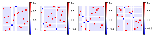
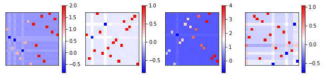
Figure 3: First row: approximate critical points of the two-layers ReLU net (4.8) with ground truth ${\bm{V}}={\bm{I}}_{20}$ and input distribution $\mathcal{D}=\mathcal{N}(0,{\bm{I}}_{20})$. The isotropy type (defined up to rows and columns permutations) coincides with the maximal isotropy groups of $\Delta S_{20}$ (see, e.g., Figure 2). Second row: approximate critical points with $({\bm{V}},\mathcal{D})$ set to $({\bm{I}}_{d/2}\oplus 2{\bm{I}}_{d/2},\mathcal{N}(0,{\bm{I}}_{20})),({\bm{I}}_{20},\mathcal{N}(0,{\bm{I}}_{d/2}\oplus{\bm{I}}_{d/2})),({\bm{I}}_{d/4}\oplus 2{\bm{I}}_{d/4}\oplus 3{\bm{I}}_{d/4}\oplus 4{\bm{I}}_{d/4},\mathcal{N}(0,{\bm{I}}_{20}))$ and $({\bm{I}}_{20},\mathcal{N}(0,{\bm{I}}_{d/4}\oplus 2{\bm{I}}_{d/4}\oplus 3{\bm{I}}_{d/4}\oplus 4{\bm{I}}_{d/4}))$, presented from left to right. The observed isotropy types adapt to the reduced joint invariance of the target model and the underlying distribution.

The least symmetry breaking principle does not always hold. A concrete counterexample, for a setting where the observed isotropy types do not match the $\Delta S_{d}$-invariance, follows by letting the underlying distribution to be $\mathcal{U}([-1+C,1+C]^{20}),~{}C\in[0,1]$. As shown by Figure 4, the symmetry of the critical points detected by SGD vanishes when $C$ approaches 1. In other cases, the principle seems to hold only partially. For example, conducting the same experiment for ReLU networks with a few fully-connected layers of constant width $d=20$ and target weights $\mathcal{V}=(\bm{1}_{20}^{\top},{\bm{I}}_{20},\dots,{\bm{I}}_{20})$ (see Definition 4.15), shows that a similar structure is apparent only at the lower levels of the network, see Figure 5.

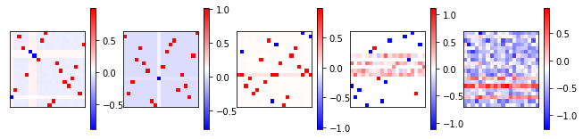
Figure 4: Critical points of the ReLU variant defined in (1.1) with an underlying distribution $\mathcal{U}([-1+C,1+C]^{20})$ where $C=0,0.25,0.5,0.75,1$, from left to right. The observed isotropy types get smaller when $C$ approaches 1.

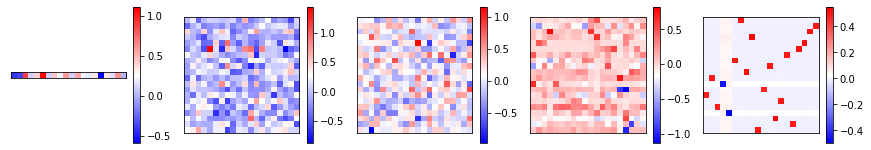
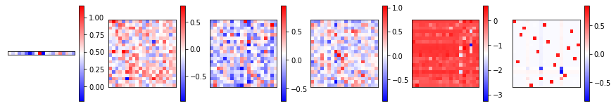
Figure 5: The weight matrices of four- and five- and six-layers fully-connected ReLU networks (the rightmost matrix corresponds to the bottom layer). The isotropy of the first and the second layers seem to be consistent with the invariance properties shown in (4.16).

6 Conclusion

In this work, we demonstrate a definite effect of the joint symmetry of various data distributions and shallow neural network architectures on the structure of critical points. In particular, the structure of spurious local minima detected by SGD in [33] are shown to be in a direct correspondence with large isotropy subgroups of the target model, suggesting a new set of complementary tools for studying loss landscapes associated with neural networks. On the flip side, so far, we have not been able to provide a rigorous proof as to why local minima tend to be highly symmetric in the settings considered in the paper. In addition, and perhaps more importantly, it is not clear at the moment how wide the phenomenon of least symmetry breaking is (e.g., Figure 4 and Figure 5), or how well it relates to realistic settings of, say, convents trained over image databases.

To conclude, the fact that a purely theoretical analysis gives a rather precise description of what is observed in practice, together with the fact that such phenomena have been encountered many times in various scientific fields are encouraging and form our main motivation for reporting these findings. Of course, isotropy analysis only characterize the landscape of generic invariant functions to a limited degree (as further demonstrated by [34]); It is for this reason that we believe that the hidden mechanism, which makes this analysis suitable for the settings considered here, merits further investigation.

7 Acknowledgments

Part of this work was completed while YA was visiting the Simons Institute for the Foundations of Deep Learning program. We thank Haggai Maron, Michelle O’Connell, Nimrod Segol, Ohad Shamir, Michal Shavit, Daniel Soudry and Alex Wein for helpful and insightful discussions.

Appendix A Proofs

A.1 Proof for Proposition 3

Proof Let $Df:E{\rightarrow}L(E,);{\bm{x}}\mapsto Df_{\bm{x}}$ denote the derivative map of $f$. It holds that for all ${\bm{x}},{\bm{e}}\in E,g\in G$

$$Df_{\bm{x}}({\bm{e}}) =\lim_{t{\rightarrow}0}\frac{f({\bm{x}}+t{\bm{e}})-f({\bm{e}})}{t}$$ (A.17)

$$=\lim_{t{\rightarrow}0}\frac{f(g({\bm{x}}+t{\bm{e}}))-f(g{\bm{e}})}{t}$$ (A.18)

$$=\lim_{t{\rightarrow}0}\frac{f(g{\bm{x}}+tg{\bm{e}})-f(g{\bm{e}})}{t}$$ (A.19)

$$=Df_{g{\bm{x}}}(g{\bm{e}}).$$ (A.20)

By definition of the gradient vector field we have for any ${\bm{e}}\in^{n}$,

$$\langle{\nabla{f}}(g{\bm{x}}),{\bm{e}}\rangle=Df_{g{\bm{x}}}({\bm{e}})=Df_{\bm{x}}(g^{-1}{\bm{e}})=\langle{\nabla{f}}({\bm{x}}),g^{-1}{\bm{e}}\rangle=\langle g^{-\top}{\nabla{f}}({\bm{x}}),{\bm{e}}\rangle.$$ (A.21)

Hence for all ${\bm{e}}\in^{n}$, $\langle{\nabla{f}}(g{\bm{x}}),{\bm{e}}\rangle=\langle g^{-\top}\,{\nabla{f}}({\bm{x}}),{\bm{e}}\rangle$ and so ${\nabla{f}}(g{\bm{x}})=g^{-\top}\,{\nabla{f}}({\bm{x}})$. In particular, if $G\subseteq{\text{\rm O}({n})}$, then $g=g^{-\top}$ and ${\nabla{f}}$ is $G$-equivariant. The rest of the properties are immediate corollaries of the $G$-equivariance of the gradient. ∎

A.2 Full Derivation of Equation 3.7

For notational convenience, we let ${\bm{U}}={\bm{W}}^{(i)}$ and ${\bm{V}}={\bm{W}}^{(i+1)}$ and focus only on these two variables. Concretely, assume $f({\bm{A}}{\bm{U}},{\bm{V}}{\bm{A}}^{-1})=f({\bm{U}},{\bm{V}})$, for any ${\bm{A}}\in{\text{\rm GL}({\mathbb{R}^{n}})}$. Define $\Pi$ to be the corresponding representation of ${\text{\rm GL}({\mathbb{R}^{n}})}$. Then,

$$\frac{\partial\Pi({\bm{A}})({\bm{U}},{\bm{V}})}{\partial{\bm{A}}}=\frac{\partial({\bm{A}}{\bm{U}},{\bm{V}}{\bm{A}}^{-1})}{\partial{\bm{A}}}=\left(\begin{array}[]{cccccccccccccccccc}{\bm{U}}^{\top}\otimes{\bm{I}}_{d_{i}}\\ -{\bm{A}}^{-\top}\otimes{\bm{V}}{\bm{A}}^{-1}\end{array}\right)$$

Thus,

$$\left.\frac{\partial\Pi({\bm{A}})({\bm{U}},{\bm{V}})}{\partial{\bm{A}}}\right|_{{\bm{A}}={\bm{I}}}=\left(\begin{array}[]{cccccccccccccccccc}{\bm{U}}^{\top}\otimes{\bm{I}}_{d_{i}}\\ -{\bm{I}}_{d_{i}}\otimes{\bm{V}}\end{array}\right).$$

On the other hand

$$D\Phi({\bm{U}},{\bm{V}})=D\left(({\bm{U}}{\bm{U}}^{\top}-{\bm{V}}^{\top}{\bm{V}})/2\right)=\left(\begin{array}[]{cccccccccccccccccc}{\bm{U}}^{\top}\otimes{\bm{I}}_{d_{i}}\\ -{\bm{I}}_{d_{i}}\otimes{\bm{V}}\end{array}\right)({\bm{I}}_{d_{i}^{2}}+{\bm{K}}_{d_{i},d_{i}}),$$

where ${\bm{K}}_{d_{i},d_{i}}$ is the respective commutation matrix (see [28, Chapter 3.7]). The rest of the proof follows mutatis mutandis.

A.3 Critical Points of $\eta$

We consider the more general real-valued function $f:\mathbb{R}^{n}\to\mathbb{R}$ defined as follows (see [21, Section 4.5.3] for a more detailed study of ${\nabla{\eta}}$ and ${\text{\rm H}_{d}}$),

$$f({\bm{x}})=\frac{a}{2}\|{\bm{x}}\|^{2}+\frac{b}{4}\|{\bm{x}}\|^{4}+\frac{c}{4}\sum^{n}_{i=1}{x_{i}^{4}}.$$ (A.22)

We have

$${\nabla{f}}({\bm{x}}) =a{\bm{x}}+b\|{\bm{x}}\|^{2}{\bm{x}}+c(x_{1}^{3},\dots,x_{n}^{3})^{\top},$$ (A.23)

$${\nabla^{2}\!{f}}({\bm{x}}) =aI+b\|{\bm{x}}\|^{2}I+2b{\bm{x}}{\bm{x}}^{\top}+3c\text{Diag}\left(x_{1}^{2},\dots,x_{n}^{2}\right).$$ (A.24)

Given $I\subset[n]$, we form a set of solutions whose zero-coordinates are specified by $I$. Indeed, assuming $\frac{-a}{b|I|+c}>0$, we set

$$x_{i}=\begin{cases}0&i\in I,\\ \sqrt{\frac{-a}{b|I|+c}}&i\notin I.\end{cases}$$

In particular, $\|{\bm{x}}\|^{2}=\frac{-a|I|}{b|I|+c}$. Therefore, for any $i\in[n]$, it follows that

$${\nabla{f}}_{i}({\bm{x}}) =x_{i}(a+b\|{\bm{x}}\|^{2}+c{x_{i}^{2}})=x_{i}\left(a-\frac{ab|I|}{b|I|+c}+c{x_{i}^{2}}\right)=\frac{x_{i}}{c}\left(\frac{a}{b|I|+c}+{x_{i}^{2}}\right)=0.$$

Clearly, any change of sign of $x_{i}$ for some $i\in I$ produces a different critical point. It is straightforward to verify that these are the only critical points which correspond to $S$. The overall number of critical points is therefore $\sum_{i=0}^{n}\binom{n}{i}2^{n-i}=3^{n}$. Moreover, it is easy to verify that the isotropy group of any critical point ${\bm{x}}\in\left\{-\sqrt{{-a}/{(b|I|+c)}},0,\sqrt{{-a}/{(b|I|+c)}}\right\}^{n}$ is conjugate to $S_{p}\times H_{n-p}$, where $p$ is the number of non-zero coordinates of ${\bm{x}}$.

Next, we compute the eigenvalues of the Hessians at the critical points of $f$ in order to determine their extremal properties. Let ${\bm{x}}\in\left\{-\sqrt{{-a}/{(b|S|+c)}},0,\sqrt{{-a}/{(b|S|+c)}}\right\}^{n}$, with at most $|S|$ nonzero entries, be a critical point and assume w.l.o.g. that the nonzero coordinates appear before the zero coordinates. Letting $M\in\mathbb{R}^{|S|\times|S|}$ be defined by $M_{ij}=\mbox{sgn}(x_{i}x_{j})$, we have by Equation A.24 that

$${\nabla^{2}\!{f}}({\bm{x}}) =aI+b\|{\bm{x}}\|^{2}I+2b{\bm{x}}{\bm{x}}^{\top}+3c\text{Diag}\left(x_{1}^{2},\dots,x_{n}^{2}\right)$$

$$=\left(a-\frac{ab|S|}{b|S|+c}\right)I-\frac{2ab}{b|S|+c}M\oplus 0_{n-|S|}-\frac{3ac}{b|S|+c}I_{|S|}\oplus 0_{n-|S|}$$

$$=\left(\frac{ac}{b|S|+c}\right)I_{|S|}\oplus I_{n-|S|}-\frac{2ab}{b|S|+c}M\oplus 0_{n-|S|}-\frac{3ac}{b|S|+c}I_{|S|}\oplus 0_{n-|S|}$$

$$=\frac{-a}{{b|S|+c}}\left[\left(2cI_{|S|}+2bM\right)\oplus-cI_{n-|S|}\right].$$

The eigenvalues of $M$ can be easily verified to be $\{|S|,0,\dots,0\}$, which implies that the eigenvalues of the Hessian are

$$\frac{-a}{{b|S|+c}}\left\{2(b|S|+c),\underbrace{2c,\dots,2c}_{|S|-1\text{ times}},\underbrace{-c,\dots,-c}_{n-|S|}\right\}.$$ (A.25)

It follows then that if $b,c>0>a$ then a critical point is extremal iff its isotropy groups is $S_{n}$ or $H_{n}$, which corresponds to a minima at $\sqrt{{-a}/{({b|S|+c})}}(\pm 1,\dots,\pm 1)$ or a maxima at ${\bm{0}}$, respectively. Additional examples for critical points of other classes of finite reflections groups, e.g., the symmetric group $S_{d}$, can be found [21].

Appendix B Complementary for Section 4

B.1 Proof of Lemma 4

$H$ acts transitively on the set of rows of $R_{ab}$. It follows that if $R$ is a row of $R_{ab}$ and $h\in H$, then for all $\ell\in[t_{ab}]$, $h:R\cap T_{\ell}^{ab}\to hR\cap T_{\ell}^{ab}$, and is a bijection. A similar proof holds for columns.

B.2 Third Examples in (4.12)

Recall our convention that the group $H_{1}$ permutes rows and $H_{2}$ permutes columns. We write elements $(\pi,\rho)\in H_{1}\times H_{2}$ as $(\pi^{r},\rho^{c})$ to emphasize this and let $e^{r}$, $e^{c}$ denote the identity elements of $H_{1}$, $H_{2}$, respectively. With these conventions, observe that $\Gamma_{\bm{W}}$ contains the seven non-trivial symmetries

$$\begin{matrix}((13)^{c}(24)^{c},(12)^{r})&((12)^{c}(34)^{c},(34)^{r})&((23)^{c}(14)^{c},(12)^{r}(34)^{r})\\ ((23)^{c},(13)^{r}(24)^{r})&((14)^{c},(14)^{4}(23)^{r})&\\ ((1342)^{c},(1324)^{r})&((3124)^{c},(3142)^{r})&\end{matrix}$$

which generate a group $H$ of order $8$, which is not isomorphic to a product (as in Lemma 4). The action of $H$ on the set of entries $w_{ij}=\alpha$ and $w_{ij}=\beta$ is transitive. If $\Gamma_{\bm{W}}(1,1)$ contains component $w_{ij}$ with a $\beta$-entry, then $\Gamma_{\bm{W}}$ must act transitively on ${[4]}^{2}$, which violates our assumption that $\alpha\neq\beta$. Therefore the only way the order of $\Gamma_{\bm{W}}$ can be greater than $8$ is if there exists $h\in\Gamma_{\bm{W}}$ which fixes $(1,1)$ but is not the identity. Necessarily, such an $h$ fixes column 1 and row 1 and preserves $\alpha,\beta$ in the complementary $3\times 3$-matrix. However, this matrix is easily seen to have trivial isotropy (within $M(3,3)$) and so $\Gamma_{\bm{W}}=H$. One can verify directly that $\Gamma_{\bm{W}}$ is isomorphic to ${\mathbb{D}}_{4}$.

B.3 Proof of Lemma 6

Proof The first statement is immediate since $H$ is transitive and so for $i\in{[k]}$, there exists $\sigma\in H$ such that $\sigma(1)=i$. Hence $(\sigma,\sigma)(1,1)=(i,i)$. The converse follows since the hypotheses imply that each row and column contain exactly one point in the $\Gamma_{\bm{W}}$-orbit of $(i_{0},j_{0})$. Hence we can permute rows and columns so that the diagonal entries are identical and differ from the off-diagonal entries (use Lemma 4). It is now easy to see that the isotropy of the permuted matrix is of diagonal type—the conjugacy with $\Gamma_{\bm{W}}$ is given by the permutation that makes the diagonal entries equal. ∎

B.4 Proof of Lemma 8

Proof (Sketch) (1) If $p=q=d/2$, we can add all permutations which map ${[p]}$ to ${[d]}\smallsetminus{[p]}$ to obtain a larger proper transitive subgroup of $S_{d}$. (2) The idea here is that the transitive partition breaks into $q$ blocks $(B_{i})_{i\in{[q]}}$ each of size $p$. Elements of the wreath product act by permuting elements in each block and then permuting the blocks (the basic wreath product structure). The order of the group is $|S_{p}|^{q}|S_{q}|=(p!)^{q}q!$. We refer the reader to [27] for details and references. ∎

References

• [1] Shun-Ichi Amari, Hyeyoung Park, and Tomoko Ozeki. Singularities affect dynamics of learning in neuromanifolds. Neural computation, 18(5):1007–1065, 2006.
• [2] Yossi Arjevani. Hidden minima in two-layer relu networks. arXiv preprint arXiv:2312.06234, 2023.
• [3] Yossi Arjevani, Joan Bruna, Michael Field, Joe Kileel, Matthew Trager, and Francis Williams. Symmetry breaking in symmetric tensor decomposition. arXiv preprint arXiv:2103.06234, 2021.
• [4] Yossi Arjevani and Michael Field. Analytic characterization of the hessian in shallow relu models: A tale of symmetry. Advances in Neural Information Processing Systems, 33:5441–5452, 2020.
• [5] Yossi Arjevani and Michael Field. Analytic study of families of spurious minima in two-layer relu neural networks: a tale of symmetry ii. Advances in Neural Information Processing Systems, 34:15162–15174, 2021.
• [6] Yossi Arjevani and Michael Field. Symmetry & critical points for a model shallow neural network. Physica D: Nonlinear Phenomena, 427:133014, 2021.
• [7] Yossi Arjevani and Michael Field. Annihilation of spurious minima in two-layer relu networks. Advances in Neural Information Processing Systems, 35:37510–37523, 2022.
• [8] Yossi Arjevani and Michael Field. Equivariant bifurcation, quadratic equivariants, and symmetry breaking for the standard representation of s k. Nonlinearity, 35(6):2809, 2022.
• [9] Yossi Arjevani and Gal Vinograd. Symmetry & critical points for symmetric tensor decompositions problems. arXiv preprint arXiv:2306.5319838, 2023.
• [10] Michael Aschbacher and Leonard Scott. Maximal subgroups of finite groups. J. Algebra, 92(1):44–80, 1985.
• [11] Johanni Brea, Berfin Simsek, Bernd Illing, and Wulfram Gerstner. Weight-space symmetry in deep networks gives rise to permutation saddles, connected by equal-loss valleys across the loss landscape. arXiv preprint arXiv:1907.02911, 2019.
• [12] Alon Brutzkus and Amir Globerson. Globally optimal gradient descent for a convnet with gaussian inputs. In Proceedings of the 34th International Conference on Machine Learning-Volume 70, pages 605–614. JMLR. org, 2017.
• [13] Alon Brutzkus, Amir Globerson, Eran Malach, and Shai Shalev-Shwartz. SGD learns over-parameterized networks that provably generalize on linearly separable data. In 6th International Conference on Learning Representations, ICLR 2018, Vancouver, BC, Canada, April 30 - May 3, 2018, Conference Track Proceedings, 2018.
• [14] Jian Ding, Allan Sly, and Nike Sun. Proof of the satisfiability conjecture for large k. In Proceedings of the Forty-Seventh Annual ACM on Symposium on Theory of Computing, STOC 2015, Portland, OR, USA, June 14-17, 2015, pages 59–68, 2015.
• [15] JohnΒ D Dixon and Brian Mortimer. Permutation groups, volume 163. Springer Science & Business Media, 1996.
• [16] SimonΒ S Du, Wei Hu, and JasonΒ D Lee. Algorithmic regularization in learning deep homogeneous models: Layers are automatically balanced. In Advances in Neural Information Processing Systems, pages 384–395, 2018.
• [17] SimonΒ S. Du, JasonΒ D. Lee, Yuandong Tian, Aarti Singh, and BarnabΓ‘s PΓ³czos. Gradient descent learns one-hidden-layer CNN: don’t be afraid of spurious local minima. In Proceedings of the 35th International Conference on Machine Learning, ICML 2018, StockholmsmΓ€ssan, Stockholm, Sweden, July 10-15, 2018, pages 1338–1347, 2018.
• [18] SimonΒ S. Du, Xiyu Zhai, BarnabΓ‘s PΓ³czos, and Aarti Singh. Gradient descent provably optimizes over-parameterized neural networks. In 7th International Conference on Learning Representations, ICLR 2019, New Orleans, LA, USA, May 6-9, 2019, 2019.
• [19] Soheil Feizi, Hamid Javadi, Jesse Zhang, and David Tse. Porcupine neural networks:(almost) all local optima are global. arXiv preprint arXiv:1710.02196, 2017.
• [20] M.Β J. Field and R.Β W. Richardson. Symmetry breaking and the maximal isotropy subgroup conjecture for reflection groups. Archive for Rational Mechanics and Analysis, 105(1):61–94, Mar 1989.
• [21] MichaelΒ J. Field. Dynamics and symmetry, volumeΒ 3 of ICP Advanced Texts in Mathematics. Imperial College Press, London, 2007.
• [22] Rong Ge, JasonΒ D. Lee, and Tengyu Ma. Learning one-hidden-layer neural networks with landscape design. In 6th International Conference on Learning Representations, ICLR 2018, Vancouver, BC, Canada, April 30 - May 3, 2018, Conference Track Proceedings, 2018.
• [23] Martin Golubitsky. The benard problem, symmetry and the lattice of isotropy subgroups. Bifurcation Theory, Mechanics and Physics. CP Boner et al., eds.(Reidel, Dordrecht, 1983), pages 225–256, 1983.
• [24] Majid Janzamin, Hanie Sedghi, and Anima Anandkumar. Beating the perils of non-convexity: Guaranteed training of neural networks using tensor methods. arXiv preprint arXiv:1506.08473, 2015.
• [25] Yuanzhi Li and Yingyu Liang. Learning overparameterized neural networks via stochastic gradient descent on structured data. In Advances in Neural Information Processing Systems, pages 8157–8166, 2018.
• [26] Yuanzhi Li and Yang Yuan. Convergence analysis of two-layer neural networks with relu activation. In Advances in Neural Information Processing Systems, pages 597–607, 2017.
• [27] MartinΒ W Liebeck, CherylΒ E Praeger, and Jan Saxl. A classification of the maximal subgroups of the finite alternating and symmetric groups. Journal of Algebra, 111(2):365–383, 1987.
• [28] JanΒ R Magnus and Heinz Neudecker. Matrix differential calculus with applications in statistics and econometrics. John Wiley & Sons, 2019.
• [29] LΒ Michel. Minima of higgs-landau polynomials. Technical report, 1979.
• [30] Emin Orhan and Xaq Pitkow. Skip connections eliminate singularities. In 6th International Conference on Learning Representations, ICLR 2018, Vancouver, BC, Canada, April 30 - May 3, 2018, Conference Track Proceedings, 2018.
• [31] Rina Panigrahy, Ali Rahimi, Sushant Sachdeva, and Qiuyi Zhang. Convergence results for neural networks via electrodynamics. In 9th Innovations in Theoretical Computer Science Conference, ITCS 2018, January 11-14, 2018, Cambridge, MA, USA, pages 22:1–22:19, 2018.
• [32] David Saad and SaraΒ A Solla. On-line learning in soft committee machines. Physical Review E, 52(4):4225, 1995.
• [33] Itay Safran and Ohad Shamir. Spurious local minima are common in two-layer relu neural networks. In Proceedings of the 35th International Conference on Machine Learning, ICML 2018, StockholmsmΓ€ssan, Stockholm, Sweden, July 10-15, 2018, pages 4430–4438, 2018.
• [34] JΓΌrgen Scheurle and Sebastian Walcher. Minima of invariant functions: The inverse problem. Acta Applicandae Mathematicae, 137(1):233–252, 2015.
• [35] Ohad Shamir. Distribution-specific hardness of learning neural networks. The Journal of Machine Learning Research, 19(1):1135–1163, 2018.
• [36] Mahdi Soltanolkotabi, Adel Javanmard, and JasonΒ D Lee. Theoretical insights into the optimization landscape of over-parameterized shallow neural networks. IEEE Transactions on Information Theory, 65(2):742–769, 2018.
• [37] Yuandong Tian. An analytical formula of population gradient for two-layered relu network and its applications in convergence and critical point analysis. In Proceedings of the 34th International Conference on Machine Learning-Volume 70, pages 3404–3413. JMLR. org, 2017.
• [38] Haikun Wei, Jun Zhang, Florent Cousseau, Tomoko Ozeki, and Shun-ichi Amari. Dynamics of learning near singularities in layered networks. Neural computation, 20(3):813–843, 2008.
• [39] BoΒ Xie, Yingyu Liang, and LeΒ Song. Diverse neural network learns true target functions. In Proceedings of the 20th International Conference on Artificial Intelligence and Statistics, AISTATS 2017, 20-22 April 2017, Fort Lauderdale, FL, USA, pages 1216–1224, 2017.
• [40] Qiuyi Zhang, Rina Panigrahy, Sushant Sachdeva, and Ali Rahimi. Electron-proton dynamics in deep learning. arXiv preprint arXiv:1702.00458, pages 1–31, 2017.
• [41] Kai Zhong, Zhao Song, Prateek Jain, PeterΒ L Bartlett, and InderjitΒ S Dhillon. Recovery guarantees for one-hidden-layer neural networks. In Proceedings of the 34th International Conference on Machine Learning-Volume 70, pages 4140–4149. JMLR. org, 2017.