Scattering-based geometric shaping of photon-photon interactions

Abstract

We construct an effective Hamiltonian of interacting bosons, based on scattered radiation off vibrational modes of designed molecular architectures. Making use of the infinite yet countable set of spatial modes representing the scattering of light, we obtain a variable photon-photon interaction in this basis. The effective Hamiltonian hermiticity is controlled by a geometric factor set by the overlaps of spatial modes. Using this mapping, we relate intensity measurements of the light to correlation functions of the interacting bosons evolving according to the effective Hamiltonian, rendering local as well as nonlocal observables accessible. This architecture may be used to simulate the dynamics of interacting bosons, as well as designing tool for multi-qubit photonic gates in quantum computing applications. Variable hopping, interaction and confinement of the active space of the bosons are demonstrated on a model system.

Quantum machines are fundamentally different from their classical counterparts (Nielsen and Chuang, 2010). Classical computers are implemented using a binary basis set. One of the benefits of this choice is minimal average energy consumption as well as minimal bit error rate in the information transmission of a noisy channel (Massoud Salehi and Proakis, 2007). For such a machine to be useful, it requires large scale integration of fundamental operations, where each level adds to the overall error rate. Deterministic intermediate quantities can be measured and corrected via feedback loops without interrupting the calculation process. In quantum machines the smallest possible unit of data (qubit) carries a phase which manifests a continuous degree of freedom. Upscaling of operations on qubits is also required for nontrivial tasks. The propagation of quantum information through such integrated system evolves errors continuously as well. This makes the realization of fault tolerant quantum processing challenging, and continues to motivate intense scientific effort (Shor, 1995; Gottesman et al., 2001; Schindler et al., 2011). Quantum simulators based on optical traps pioneered by Cirac and Zoller (Cirac and Zoller, 1995; Jaksch et al., 1998) have matured experimentally (Monroe, 2002; Kim et al., 2010). They are widely used in the study of quantum dynamics such as spin frustration (Kim et al., 2010) and thermalization and localization transitions (Schreiber et al., 2015; Smith et al., 2016). Recently more applications of lattice gauge theories have been proposed, appealing to simulations of high energy physics (Zohar et al., 2015; Rico et al., 2018; Muschik et al., 2017). While these fascinating quantum simulators offer unprecedented glimpse into nonequilibrium dynamics, upscaling the number of qubits is just as challenging.

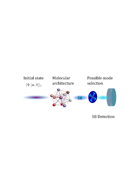
Figure 1: Proposed realization of the geometric SPC. The incident beam is scattered-off a molecular architecture, realizing interaction between its spatial components denoted SB. A single mode as well as any combination of such are addressable, rendering projective measurement in the chosen basis possible. The SBs can be mapped into discrete lattice sites for which cross-correlations can be constructed using the photon-statistics.

Here we propose a Geometric scattering-based Spatial Photon Coupler (SPC) that can be used to simulate quantum dynamics of interacting bosons. The setup is depicted in Fig.$\left(\text{\ref{fig:Setup}}\right)$, and based on off-resonant scattering of photons on geometrically arranged distribution of molecules. We show that the scattering process can be mapped into the effective Hamiltonian,

$$H_{eff}=\sum_{nk}\Theta_{nk}a_{n}^{\dagger}a_{k}-\sum_{nklm}U_{nklm}a_{n}^{\dagger}a_{k}a_{l}^{\dagger}a_{m},$$ (1)

where $a_{k}\left(a_{k}^{\dagger}\right)$ is a discrete bosonic annihilation (creation) operator. The hopping $\left(\Theta_{nk}\right)$ and the interaction $\left(U_{nklm}\right)$ terms are determined by three main quantities: (1) the geometry (design) of the microscopic building blocks (2) their internal structure (spectrum) (3) the measurement basis chosen. It holds two significant advantages. First, it can be designed to maintain hermiticity such that marginal losses in photon number occur , inelastic contributions in this case result in frequency shift of the incident photon. Second, while the number of connected modes is infinite, it can be confined with intelligent design. Our goal is to shape the induced dynamics constrained by the Hamiltonian in Eq.$\left(\text{\ref{Effective Hamiltoian}}\right)$ then read the encoded information from the final photonic wavefunction,

$$|\Psi\left[\boldsymbol{n},\tau\right]\rangle_{f}=e^{-iH_{eff}\tau}|\Psi\left[\boldsymbol{n},0\right]\rangle_{i}.$$ (2)

Intensity measurements reveal the Scattered Bosons (SBs) densities $\hat{n}_{k}\equiv a_{k}^{\dagger}a_{k}$, evolving on a network (graph) of a topology imposed by $H_{eff}$ connectivity as depicted in Fig.$\left(\text{\ref{fig:Setup}}\right)$. $\tau$ denotes the interaction time, beyond which $U_{nklm}\equiv 0$.

We consider arbitrary initial superposition of spatial modes, reflecting some initial (multiple-photon) distribution of SBs. One possibility of particular interest to the simulation of interacting bosons, is a (normalized) product of $N$ single photon states $|\boldsymbol{1}\rangle=\sum_{n}{\cal C}_{n}a_{n}^{\dagger}|0\rangle$, corresponding to initially noninteracting bosons. One way to achieve that is by direct state preparation. Another is via two-mode spontaneous parametric down converter source in which one photon is scattered while the other serves as the Reference for the SB (RSB) as was done in Asban et al. (2019) and inspired by (Fickler et al., 2016, 2012; Krenn et al., 2013; Bavaresco et al., 2018; Straupe et al., 2011), see . In both manifestations, the RSBs are used to extract the SBs statistics which is first scattered as depicted in Fig $\left(\text{\ref{fig:Setup}}\right)$. Surveying the SBs statistics using cross-correlations with RSBs, renders "local" $\propto\left\langle\hat{n}_{r}\left(\tau\right)\right\rangle$ and $\left\langle\hat{n}_{r}\left(0\right)\hat{n}_{r}\left(\tau\right)\right\rangle$, as well as "nonlocal" quantities $\propto\sum_{R}\left\langle\hat{n}_{r}\left(0\right)\hat{n}_{r+R}\left(\tau\right)\right\rangle$ accessible. While conventional quantum simulators are limited by the number of physical qubits, the proposed geometric SPC benefits from controlled - potentially infinite - number of participating modes. These characteristics are highly desirable for simulating thermodynamic properties of interacting particles.

Constructing the effective Hamiltonian. Off-resonant light-matter interaction is given by the minimal coupling Hamiltonian,

$$H_{\mu\phi}=\int d\boldsymbol{r}\sigma\left(\boldsymbol{r},t\right)\boldsymbol{A}^{2}\left(\boldsymbol{r},t\right),$$ (3)

where $\mu$ and $\phi$ denote the matter and photon fields respectively. Radiation modes interaction is mediated by the charge-density operator $\sigma\left(\boldsymbol{r}\right)$. The vector potential in the paraxial approximation takes the form $\boldsymbol{A}_{p}\left(\boldsymbol{r},t\right)=\sum_{\sigma,l,p}\underset{0}{\overset{\infty}{\int}}dk_{0}C\left(k_{0}\right)\left[A_{\sigma lp}^{\left(+\right)}\left(k_{0}\right)e^{ik_{0}\left(z-ct\right)}+h.c.\right],$ where $k_{0}$ is the wavector in the longitudinal direction, $C\left(k_{0}\right)=\left(\nicefrac{{1+\vartheta^{2}}}{{16\pi^{3}\varepsilon_{0}k_{0}}}\right)^{\nicefrac{{1}}{{2}}}$ and $\vartheta=\nicefrac{{q}}{{\sqrt{2k_{0}^{2}}}}$ is the degree of paraxiality (Aiello and Woerdman, 2005; Calvo et al., 2006). The vector potential operator is defined by $A_{\sigma lp}^{\left(+\right)}\left(k_{0}\right)=\epsilon_{\sigma}\hat{a}_{\sigma,l,p}\left(k_{0}\right)\psi_{l,p}\left(\boldsymbol{\rho},z;k_{0}\right)$ where $\hbar=c=1$. $\boldsymbol{\rho}$ is the polar distance (cylindrical coordinates) and the indices $l,p$ label the spatial basis set $\psi_{lp}\left(\boldsymbol{\rho},z;k_{0}\right)$ [in (Aiello and Woerdman, 2005; Calvo et al., 2006) Laguerre-Gauss (LG) basis is used]. Any complete basis which is a solution of the paraxial equation, such as Hermite- or Ince-Gauss (HG,IG) can be used. Here $\epsilon_{\sigma}=\nicefrac{{\left(\boldsymbol{u}_{x}-i\sigma\boldsymbol{u_{y}}\right)}}{{\sqrt{2}}}$ is the polarization vector [circular for LG modes (linear for HG)] and $\sigma=\pm 1$. The field (creation/annihilation) operators in the paraxial basis satisfy the canonical commutation relations, $\left[\hat{a}_{\sigma,l,p}\left(k_{0}\right),\hat{a}_{\sigma^{\prime},l^{\prime},p^{\prime}}^{\dagger}\left(k_{0}^{{}^{\prime}}\right)\right]=\delta_{\sigma\sigma^{\prime}}\delta_{ll^{\prime}}\delta_{pp^{\prime}}\delta\left(k_{0}-k_{0}^{{}^{\prime}}\right)$. The paraxial basis is given by the transformation of the standard operators $\hat{a}_{\sigma,l,p}\left(k_{0}\right)=\int d^{2}\boldsymbol{q}\phi_{lp}^{*}\left(\boldsymbol{q}\right)\hat{a}_{\sigma}\left(\boldsymbol{q}\right).$ This basis has the following properties,

$$\sum_{l,p}\phi_{lp}^{*}\left(\boldsymbol{q}\right)\psi_{lp}\left(\boldsymbol{\rho},z,k_{0}\right) = e^{i\boldsymbol{q}\cdot\boldsymbol{\rho}-k_{0}\vartheta^{2}z}$$ (4a)

$$\int d^{2}\boldsymbol{q}\phi_{lp}^{*}\left(\boldsymbol{q}\right)\phi_{mn}\left(\boldsymbol{q}\right) = \delta_{lm}\delta_{pn}$$ (4b)

$$\sum_{l,p}\phi_{lp}^{*}\left(\boldsymbol{q}\right)\phi_{lp}\left(\boldsymbol{q}^{\prime}\right) = \delta\left(\boldsymbol{q}-\boldsymbol{q}^{\prime}\right)$$ (4c)

where $\boldsymbol{q}$ is the transverse momentum and $\phi_{lp}\left(\boldsymbol{q}\right)$ is the LG spatial modes Fourier transform taken at $z=0$. The full Hamiltonian is given by ${\cal H}=H_{0}+H_{\mu\phi}$, where $H_{0}=H_{\phi}+H_{\mu}$ is the noninteracting Hamiltonian of the radiation $\left(\phi\right)$ and matter $\left(\mu\right)$. With these notations, the interaction Hamiltonian can be recast in the form,

$$H_{\mu\phi} =\sum_{\boldsymbol{k}\boldsymbol{q}}\sigma_{\boldsymbol{k}-\boldsymbol{q}}^{\dagger}a_{\boldsymbol{k}}^{\dagger}a_{\boldsymbol{q}}+\sigma_{\boldsymbol{k}-\boldsymbol{q}}a_{\boldsymbol{k}}a_{\boldsymbol{q}}^{\dagger},$$ (5)

where the highly oscillating terms corresponding to $a_{\boldsymbol{k}}a_{\boldsymbol{q}}$ and $a_{\boldsymbol{k}}^{\dagger}a_{\boldsymbol{q}}^{\dagger}$ are neglected. The matter Hamiltonian is given by $H_{\mu}=\sum_{\alpha,i}\epsilon_{i,\alpha}c_{i,\alpha}^{\dagger}c_{i,\alpha}$, where $c_{i,\alpha}\left(c_{i,\alpha}^{\dagger}\right)$ is the bosonic annihilation (creation) operator with the canonical commutation relations $\left[c_{i,\alpha},c_{j,\beta}^{\dagger}\right]=\delta_{\alpha\beta}\delta_{i,j}$. The vibrational modes labeled $i$, and scatters by $\alpha$. The charge-density operator reads $\sigma_{\boldsymbol{k}}=\sum_{\alpha=1}^{N}f_{\alpha}\left(\boldsymbol{k}\right)c_{i,\alpha}^{\dagger}c_{j,\alpha},$ where $f_{\alpha}\left(\boldsymbol{k}\right)=e^{i\boldsymbol{k}\cdot\boldsymbol{r}_{\alpha}}w\left(\boldsymbol{k}\right)$, $w\left(\boldsymbol{k}\right)$ are the localized molecular orbital and $\boldsymbol{r}_{\alpha}$ are scatterers positions. We then calculate the effective photon-photon interaction using the Schrieffer-Wolff transformation [see appendix (B.1) for detailed derivation], follows by a transformation of the momentum representation into superposition the SBs.

The SB representation. Using the above definitions for the Bogoliubov transformation from momentum space to the Schmidt representation $a_{\boldsymbol{k}}=\sum_{n}\phi_{n}\left(\boldsymbol{k}\right)a_{n},$ where $a_{n}$ is the Schmidt boson annihilation operator and $n$ is a shorthand notation for the two quantum numbers $l,p$ introduced in the expression for the vector potential. The free Hamiltonian reads assuming a single longitudinal mode at $\omega_{0}$ we get $H_{\phi}=\omega_{0}\sum_{n}a_{n}^{\dagger}a_{n}.$ The off-diagonal contributions to Eq.$\left(\text{\ref{Effective Hamiltoian}}\right)$ - namely, the hopping terms - are given by (see appendix for detailed derivation),

$$\hat{t}_{coh} =\sum_{nm}\theta_{nm}^{coh}a_{n}^{\dagger}a_{m}+h.c.,$$ (6a)

$$\hat{t}_{inc} =\sum_{nm}\theta_{nm}^{inc}\left(\Delta_{i}\right)a_{n}^{\dagger}a_{m}+\theta_{nm}^{inc*}\left(-\Delta_{i}\right)a_{m}^{\dagger}a_{n},$$ (6b)

with the hopping coefficients are,

$$\theta_{nm}^{coh} =2\sum_{\alpha\neq\beta}\sum_{\boldsymbol{k},\boldsymbol{q},\boldsymbol{s}}e^{-i\boldsymbol{\left(k-\boldsymbol{q}\right)}\cdot\boldsymbol{r}_{\alpha}+i\left(\boldsymbol{s}-\boldsymbol{q}\right)\cdot\boldsymbol{r}_{\beta}}$$ (7a)

$$\times \frac{\phi_{n}^{*}\left(\boldsymbol{k}\right)w_{\alpha}^{*}\left(\boldsymbol{k}-\boldsymbol{q}\right)w_{\beta}\left(\boldsymbol{s}-\boldsymbol{q}\right)\phi_{m}\left(\boldsymbol{s}\right)}{q^{2}-k^{2}},$$

$$\theta_{nm}^{inc} \left(\Delta_{i}\right)=2\sum_{\alpha}\sum_{\boldsymbol{k},\boldsymbol{q},\boldsymbol{s}}e^{-i\left(\boldsymbol{k}-\boldsymbol{s}\right)\cdot\boldsymbol{r}_{\alpha}}$$ (7b)

$$\times \frac{\phi_{n}^{*}\left(\boldsymbol{k}\right)w_{\alpha}^{*}\left(\boldsymbol{k}-\boldsymbol{q^{\prime}}\right)w_{\alpha}\left(\boldsymbol{q}-\boldsymbol{q}^{\prime}\right)\phi_{m}\left(\boldsymbol{s}\right)}{q^{\prime 2}-\left(k^{2}+\Delta_{i}\right)},$$

and $\Delta_{i}=2\omega_{0}\epsilon_{ig}$. Assuming a slowly varying orbital in momentum domain (point particle limit), significantly simplifies Eqs.$\left(\text{\ref{eq:exact coh}},\text{\ref{eq:Exact inc}}\right)$. When the inter-particle distance is much smaller than the transverse wavector $r_{\alpha\beta}\ll\lambda_{\perp}$, the coherent hopping [Eq.$\left(\text{\ref{eq:exact coh}}\right)$] is granted an intuitive form, carrying spatial contributions due to the phase-difference of scattered modes. Introducing a cutoff frequency $\Lambda$ such that $\nicefrac{{\left|r_{\beta\alpha}\right|}}{{\Lambda}}\leq\left|r_{\beta\alpha}\right|k\ll 1$ and $q>\nicefrac{{1}}{{\Lambda}}$ we obtain,

$$\theta_{nm}^{coh} =g^{coh}\sum_{\alpha\neq\beta}\psi_{n}^{*}\left(\boldsymbol{r}_{\alpha}\right)\psi_{m}\left(\boldsymbol{r}_{\beta}\right),$$ (8a)

$$\theta_{nk}^{inc}=g^{inc}\sum_{\alpha}\psi_{n}^{*}\left(r_{\alpha}\right)\psi_{k}\left(r_{\alpha}\right).$$ (8b)

Note that these approximations are not essential yet grant important intuition; see appendix B for the exact expressions. The over-all SB hopping coefficient is given by $\Theta_{nk}=\omega_{0}\left(\delta_{nk}-\theta_{nk}^{coh}-\theta_{nk}^{inc}\right)$.

The interaction term in Eq.$\left(\text{\ref{Effective Hamiltoian}}\right)$ can be displayed in a form that separates the geometrical factor from the basis dependent one $U_{nmls}=-\sum_{l^{{}^{\prime}}s^{{}^{\prime}}}S_{ll^{{}^{\prime}}ss^{{}^{\prime}}}V_{nml^{{}^{\prime}}s^{{}^{\prime}}}$. Here $V_{nlkm}$ is the basis dependent four-mode scattering potential,

$$V_{nlkm} =\sum_{i}\int d^{2}\boldsymbol{k}d^{2}\boldsymbol{q}\>\phi_{n}^{*}\left(\boldsymbol{k}\right)\phi_{k}\left(\boldsymbol{k}\right)$$ (9)

$$\times \left[\frac{1}{k^{2}-q^{2}-\Delta_{i}}-\frac{1}{k^{2}-q^{2}+\Delta_{i}}\right]\phi_{l}\left(\boldsymbol{q}\right)\phi_{m}^{*}\left(\boldsymbol{q}\right),$$

and the geometric structural tensor, $S_{ll^{{}^{\prime}}ss^{{}^{\prime}}}=\sum_{\alpha}f_{ll^{\prime}}^{\alpha*}f_{ss^{\prime}}^{\alpha},$ using concatenation of basis $\leftrightarrow$ geometry transformation $f_{nm}^{\alpha}=\psi_{n}^{*}\left(r_{\alpha}\right)\psi_{m}\left(r_{\alpha}\right)$ - isolating basis dependent properties from the geometric characteristics. The effective hamiltonian is finally given by Eq.$\left(\text{\ref{Effective Hamiltoian}}\right)$.

(a)

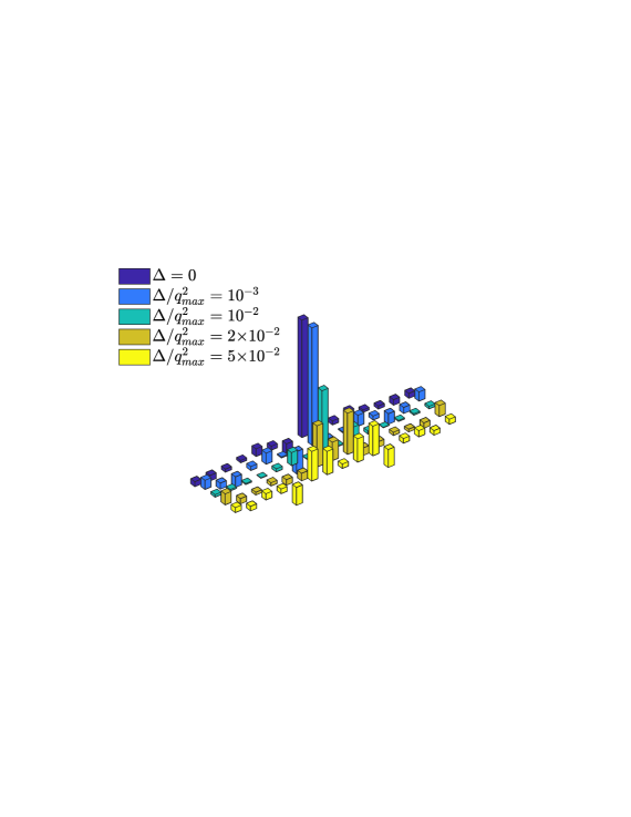
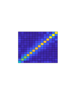
(b)(c)

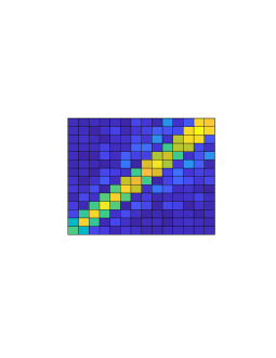
(d)(e)

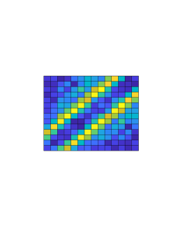
Figure 2: The scattering potential. $V_{nmkl}$ in Eq.$\left(\text{\ref{4-modes Scattering potential}}\right)$ calculated in the LG basis. Each panel corresponds to different $\Delta$ value, and panel (a) captures a summary of the diagonal crossection from the top-left to bottom-right of panels b:e. Panels b:e capture the inter-mode coupling [relations between the two middle dimensions $\left(V_{mk}=tr_{nl}V_{nmkl}\right)$], of the effective SBs scattering potential for the selected values $\nicefrac{{\Delta}}{{\boldsymbol{q}_{max}^{2}}}=\left(0.001,0.01,0.02,0.05\right)$. The calculated relations between the first two $\left(V_{nm}=tr_{kl}V_{nmkl}\right)$ and last dimensions $\left(V_{kl}=tr_{nm}V_{nmkl}\right)$ are indistinguishable from panel (b) for all values of $\Delta$ and resemble a Kronecker delta distribution.

The scattering potential in the Laguerre-Gauss basis. The target effective interaction to be simulated is manipulated and designed using three main ingredients. (i) One is purely geometric and defined by the arrangement of charges, (ii) the internal structure of each charge $\left(\Delta_{i}\right)$ and (iii) the choice of basis. While the geometric component appears in the expressions for both, the interaction and hopping terms, the charge spectral structure contributes to the scattering potential of Eq.$\left(\text{\ref{4-modes Scattering potential}}\right)$ alone. We now study the effects of $\Delta$ on the interaction which is basis dependent yet geometry independent. The scattering potential $V_{nklm}$ involves coupling between four modes. Eq.$\left(\text{\ref{4-modes Scattering potential}}\right)$ can be further simplified using the LG basis [see Eq.$\left(35B\right)$ of the supplementary material]. The structure of the scattering potential as a function of $\Delta$ for a two level system is depicted in Fig. $\left(\text{\ref{LG scattering-potential}}\right)$. For all values of $\Delta,$the relation between the first and last two modes [$n,k$ and $l,m$ of Eq.$\left(\text{\ref{Effective Hamiltoian}}\right)$] resembles a Kronecker delta . It is given by the partial traces $V_{nm}=tr_{kl}V_{nmkl}\approx\delta_{nm}$ and $V_{kl}=tr_{nm}V_{nmkl}\approx\delta_{kl}$ and depicted in Fig.$\left(\text{\ref{LG scattering-potential}}a\right)$. This property simplifies the effective Hamiltonian to,

$$H_{eff}^{LG}=\sum_{n,k}\Theta_{nk}a_{n}^{\dagger}a_{k}-\sum_{nk}\mathcal{U}_{nk}\hat{n}_{n}\hat{n}_{k},$$ (10)

where $\hat{n}_{k}=a_{k}^{\dagger}a_{k}$ is the number operator, and ${\cal U}_{nk}=\sum_{lm}U_{nlkm}\delta_{nl}\delta_{km}$. The effective potential between the first and last two modes of Eq.$\left(\text{\ref{Effective Hamiltoian}}\right)$ spreads to neighboring modes with increasing values of $\nicefrac{{\Delta}}{{\boldsymbol{q}_{max}^{2}}}$ where $\boldsymbol{q}_{max}$ is the cutoff wavector in the numerical calculation. This behavior is summarized in Fig.$\left(\text{\ref{LG scattering-potential}}a\right)$, and demonstrated separately for the selected values in Fig.$\left(\text{\ref{LG scattering-potential}}b:e\right)$. At large values of $\nicefrac{{\Delta}}{{\boldsymbol{q}_{max}^{2}}}$ the scattering occurs between more distant modes, corresponding to energy exchange with the matter. Extension of this result to a system of charges composed of a more complex internal structure, is given by a straightforward summation, resulting in longer-range interaction.

Illustrative example of the effective Hamiltonian. We derive the effective Hamiltonian for molecules in cylindrical architecture, in which controlled hopping can confine the dynamics to a restricted subspace. We consider a uniform distribution of molecules filling a hollow-cylinder (UC) of inner radius $a$ and outer radius $b$ as shown in Fig.$\left(\text{\ref{fig:Illustrative-example Uniform cylinder sketch}}\right)$. The boundary radius $c$ is defined such that 95% of the power of the incident radial mode for which $n=25$ is contained within the calculation range of the numerical simulation (the chosen cutoff mode).

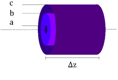
Figure 3: Uniformly distributed hollow-cylinder. Inner and outer radius $a$ and $b$ respectively, $c$ is chosen such that 95% of the power of the radial mode for which $n=25$ is contained within. $\Delta z$ is the region in which the interaction and hopping occur, corresponding to the interaction time interval $\tau$.

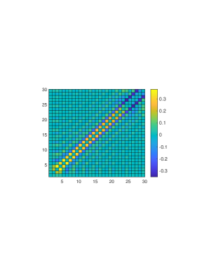
(a)(b)

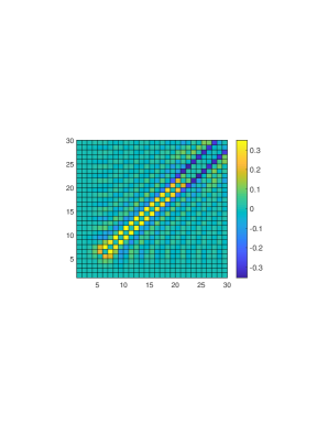
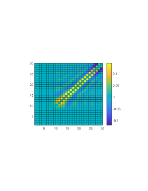
(c)(d)

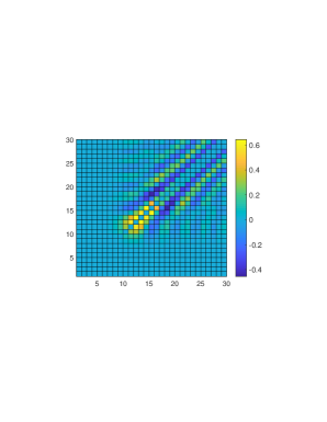
Figure 4: Geometrically controlled hopping confinement. (a-d) The geometric hopping factors $\theta_{nk}^{inc}$ presented in Eq.$\left(\text{\ref{eq:Incoherent hopping term}}\right)$ are displayed for the above geometry. Panels a-d computed with the corresponding dimensionless distance from the origin $\left(\nicefrac{{a}}{{c}},\nicefrac{{b}}{{c}}\right)$: $\left[\text{a}\left(0.1,0.9\right),\text{b}\left(0.2,0.8\right),\text{c}\left(0.4,1\right),\text{d}\left(0.4,0.6\right)\right]$. Positive contributions are energetically favorable.

In this case the geometric coefficient of the hopping terms in Eqs.$\left(\text{\ref{eq:coherent hopping term}},\text{\ref{eq:Incoherent hopping term}}\right)$ as well as the interaction can be used to confine the dynamics in a controlled subspace. By varying $a$ and $b$, the hopping range depicted in Figs.$\left(\text{\ref{fig:Hopping term from Uniform cylinder}}\right)$ a:d can be controlled. Fig.$\left(\text{\ref{fig:Hopping term from Uniform cylinder}}\right)$ along with Eqs.$\left(\text{\ref{eq:coherent hopping term}},\text{\ref{eq:Incoherent hopping term}}\right)$ show that hopping within the set of modes corresponding to positive geometric factor, is energetically favorable. These positive contributions are surrounded by negative ones which are costly energetically, resulting in effective confinement. In this setup the single-molecule field scattering presented in Eq.$\left(\text{\ref{eq:Incoherent hopping term}}\right)$ dominates the hopping dynamics and the coherent hopping term of Eq.$\left(\text{\ref{eq:coherent hopping term}}\right)$ is suppressed. This is verified by the vanishing structure factor in a disordered lattice, or equivalently from the closure relations of the LG basis combined with orthogonality [Eqs.$\left(\text{\ref{Closure}},\text{\ref{Orthonormality}}\right)$]. Using Eq.$\left(\text{\ref{Complex exponent span}}\right)$ one can estimate that for $\left|\boldsymbol{q}_{max}\right|=10^{-p}k_{0}$ and $\Delta z=10^{l}\lambda_{0}$ the modal attenuation factor is $\exp\left(-2\pi 10^{l-2p}\right)$ which yields $\approx 94\%$ of the incoming photon flux at the output for $l=p=2$. This geometry simulates the dynamics of the Hamiltonian $H_{eff}^{LG}=H_{UC}$,

$$H_{UC}=\sum_{\left\langle n,k\right\rangle\in{\cal D}_{h}}\Theta_{nk}a_{n}^{\dagger}a_{k}-\sum_{n,k\in{\cal D}_{\Delta}}\mathcal{U}_{nk}\hat{n}_{n}\hat{n}_{k},$$ (11)

where $\left\langle n,k\right\rangle$ stands for nearest neighbors. ${\cal D}_{h}$ is a domain determined by the geometry in which the hopping occurs, as shown in Fig.$\left(\text{\ref{fig:Hopping term from Uniform cylinder}}\right)$. ${\cal D}_{\Delta}$ is the domain set by $\Delta$ for which several illustrations are depicted in Fig.$\left(\text{\ref{LG scattering-potential}}\right)$.

Discussion. We have developed a geometric SPC, shaping photon-photon interactions via geometric design of the coupling between spatial modes, using the setup depicted in Fig.$\left(\text{\ref{fig:Setup}}\right)$. Quantum dynamics of interacting bosons described by the Hamiltonian of Eq.$\left(\text{\ref{Effective Hamiltoian}}\right)$ can be simulated and directly measured using the above ingredients.

The dynamics of the SBs constrained by the Eq.$\left(\text{\ref{Effective Hamiltoian}}\right)$ is controlled by the following three main quantities. The geometric distribution of molecules, their internal structure and the choice of spatial basis. The dynamics induced by the geometric SPC depicted in Fig.$\left(\text{\ref{fig:Illustrative-example Uniform cylinder sketch}}\right)$ can be restricted to a finite set of modes as demonstrated in Fig.$\left(\text{\ref{fig:Hopping term from Uniform cylinder}}\right)$. This offers a purpose-computing platform to a class of problems with exponential complexity. There is a growing interest in purpose machines, built for the solution of a specific task, e.g. coherent Ising machines (Inagaki et al., 2016; McMahon et al., 2016). These structures are designed to solve efficiently Ising models on graphs with programmable connectivity. Their usefulness stems from the well known mapping between the Ising model ground state search problem, and combinatorial optimization problems in polynomial time (Barahona, 1982) (both NP hard). The proposed setup is also applicable as a quantum (light) state-preparation technique, as well as multi-photon gate in a photonic quantum processor.

In molecular systems the number of vibrational modes $N_{vib}$ is proportional to the number of atoms $N_{a}$ according to $N_{vib}=3N_{a}-6$. The number of electronic states corresponds to the number of electrons $N_{e}$. Good candidates would be systems containing few vibrational modes while large number of electrons that potentially provide strong coupling of the vibrational modes with applied electromagnetic field. Short wavelength tabletop X-ray sources that couple off-resonantly between the vibrational modes provide intriguing possibility for source realization Rocca (2016). Longer wavelength sources for which sophisticated measurement techniques are more mature may be possible although the coupling between the modes may take more complicated forms.

Due to the structure of the LG modes, for low number of ordered scatterers, sign-flipping anti-ferromagnetic coupling has been observed that requires further characterization. Finding the molecular distribution and basis emulating the desired dynamics provides a topic for future study as well as coupling to electronic states rather than the vibrational. For this purpose, another degree of the geometric properties could be considered, the local charge distribution of a each scatterer presented in Eqs.$\left(\text{\ref{eq:exact coh},\ref{eq:Exact inc}}\right)$.

Acknowledgments. The support of the Chemical Sciences, Geosciences, and Biosciences Division, Office of Basic Energy Sciences, Office of Science, U.S. Department of Energy is gratefully acknowledged. S.M was supported by Award DE-FG02-04ER15571. S.A fellowship was supported by the National Science Foundation (Grant No. CHE-1663822).

References

- Nielsen and Chuang (2010) M. A. Nielsen and I. L. Chuang, Quantum Computation and Quantum Information: 10th Anniversary Edition (Cambridge University Press, 2010).
- Note (1) Assuming voltage levels are assigned to bit states, having ’0’ represented by zero voltage.
- Massoud Salehi and Proakis (2007) P. Massoud Salehi and J. Proakis, Digital Communications (McGraw-Hill Education, 2007).
- Shor (1995) P. W. Shor, Scheme for reducing decoherence in quantum computer memory, Phys. Rev. A 52, R2493 (1995).
- Gottesman et al. (2001) D. Gottesman, A. Kitaev, and J. Preskill, Encoding a qubit in an oscillator, Phys. Rev. A 64, 12310 (2001).
- Schindler et al. (2011) P. Schindler, J. T. Barreiro, T. Monz, V. Nebendahl, D. Nigg, M. Chwalla, M. Hennrich, and R. Blatt, Experimental Repetitive Quantum Error Correction, Science 332, 1059 (2011).
- Cirac and Zoller (1995) J. I. Cirac and P. Zoller, Quantum Computations with Cold Trapped Ions, Phys. Rev. Lett. 74, 4091 (1995).
- Jaksch et al. (1998) D. Jaksch, C. Bruder, J. I. Cirac, C. W. Gardiner, and P. Zoller, Cold Bosonic Atoms in Optical Lattices, Phys. Rev. Lett. 81, 3108 (1998).
- Monroe (2002) C. Monroe, Quantum information processing with atoms and photons, Nature 416, 238 (2002).
- Kim et al. (2010) K. Kim, M.-S. Chang, S. Korenblit, R. Islam, E. E. Edwards, J. K. Freericks, G.-D. Lin, L.-M. Duan, and C. Monroe, Quantum simulation of frustrated Ising spins with trapped ions, Nature 465, 590 (2010).
- Schreiber et al. (2015) M. Schreiber, S. S. Hodgman, P. Bordia, H. P. Lüschen, M. H. Fischer, R. Vosk, E. Altman, U. Schneider, and I. Bloch, Observation of many-body localization of interacting fermions in a quasirandom optical lattice, Science 349, 842 (2015).
- Smith et al. (2016) J. Smith, A. Lee, P. Richerme, B. Neyenhuis, P. W. Hess, P. Hauke, M. Heyl, D. A. Huse, and C. Monroe, Many-body localization in a quantum simulator with programmable random disorder, Nature Physics 12, 907 (2016).
- Zohar et al. (2015) E. Zohar, J. I. Cirac, and B. Reznik, Quantum simulations of lattice gauge theories using ultracold atoms in optical lattices, Reports on Progress in Physics 79, 14401 (2015).
- Rico et al. (2018) E. Rico, M. Dalmonte, P. Zoller, D. Banerjee, M. Bogli, P. Stebler, and U.-J. Wiese, So(3) "nuclear physics" with ultracold gases, Annals of Physics 393, 466 (2018).
- Muschik et al. (2017) C. Muschik, M. Heyl, E. Martinez, T. Monz, P. Schindler, B. Vogell, M. Dalmonte, P. Hauke, R. Blatt, and P. Zoller, U(1) wilson lattice gauge theories in digital quantum simulators, New Journal of Physics 19, 103020 (2017).
- Note (2) In linear order of the paraxiality parameter there are no losses in the longitudinal modes. Losses in the transverse modes are governed solely by the geometry. Higher orders exhibit losses and demonstrated in the illustration below.
- Asban et al. (2019) S. Asban, K. E. Dorfman, and S. Mukamel, Quantum phase-sensitive diffraction and imaging using entangled photons, Proceedings of the National Academy of Sciences 116, 11673 (2019), https://www.pnas.org/content/116/24/11673.full.pdf .
- Fickler et al. (2016) R. Fickler, G. Campbell, B. Buchler, P. K. Lam, and A. Zeilinger, Quantum entanglement of angular momentum states with quantum numbers up to 10,010, Proceedings of the National Academy of Sciences 113, 13642 (2016), arXiv:1607.00922 .
- Fickler et al. (2012) R. Fickler, R. Lapkiewicz, W. N. Plick, M. Krenn, C. Schaeff, S. Ramelow, and A. Zeilinger, Quantum Entanglement of High Angular Momenta, Science 338, 640 (2012).
- Krenn et al. (2013) M. Krenn, R. Fickler, M. Huber, R. Lapkiewicz, W. Plick, S. Ramelow, and A. Zeilinger, Entangled singularity patterns of photons in Ince-Gauss modes, Phys. Rev. A 87, 12326 (2013).
- Bavaresco et al. (2018) J. Bavaresco, N. Herrera Valencia, C. Klöckl, M. Pivoluska, P. Erker, N. Friis, M. Malik, and M. Huber, Measurements in two bases are sufficient for certifying high-dimensional entanglement, Nature Physics 14, 1032 (2018).
- Straupe et al. (2011) S. S. Straupe, D. P. Ivanov, A. A. Kalinkin, I. B. Bobrov, and S. P. Kulik, Angular schmidt modes in spontaneous parametric down-conversion, Phys. Rev. A 83, 060302(R) (2011).
- Note (3) Using entangled photon pair such that the as SB and RSB ideally results in background free signal yet harder to produce.
- Aiello and Woerdman (2005) A. Aiello and J. P. Woerdman, Exact quantization of a paraxial electromagnetic field, Phys. Rev. A 72, 060101(R) (2005).
- Calvo et al. (2006) G. F. Calvo, A. Picon, and E. Bagan, Quantum field theory of photons with orbital angular momentum, Phys. Rev. A 73, 013805 (2006).
- Inagaki et al. (2016) T. Inagaki, Y. Haribara, K. Igarashi, T. Sonobe, S. Tamate, T. Honjo, A. Marandi, P. L. McMahon, T. Umeki, K. Enbutsu, O. Tadanaga, H. Takenouchi, K. Aihara, K.-i. Kawarabayashi, K. Inoue, S. Utsunomiya, and H. Takesue, A coherent Ising machine for 2000-node optimization problems, Science 354, 603 (2016).
- McMahon et al. (2016) P. L. McMahon, A. Marandi, Y. Haribara, R. Hamerly, C. Langrock, S. Tamate, T. Inagaki, H. Takesue, S. Utsunomiya, K. Aihara, R. L. Byer, M. M. Fejer, H. Mabuchi, and Y. Yamamoto, A fully programmable 100-spin coherent Ising machine with all-to-all connections, Science 354, 614 (2016).
- Barahona (1982) F. Barahona, On the computational complexity of Ising spin glass models, Journal of Physics A: Mathematical and General 15, 3241 (1982).
- Rocca (2016) J. J. Rocca, Table-top soft x-ray lasers, in Conference on Lasers and Electro-Optics (Optical Society of America, 2016) p. AM1K.1.