Spectral fluctuations in the Sachdev-Ye-Kitaev model

Abstract

We present a detailed quantitative analysis of spectral correlations in the Sachdev-Ye-Kitaev (SYK) model. We find that the deviations from universal Random Matrix Theory (RMT) behavior are due to a small number of long-wavelength fluctuations (of the order of the number of Majorana fermions $N$) from one realization of the ensemble to the next one. These modes can be parameterized effectively in terms of Q-Hermite orthogonal polynomials, the main contribution being due to scale fluctuations for which we give a simple analytical estimate. Our numerical results for $N=32$ show that only the lowest eight polynomials are needed to eliminate the nonuniversal part of the spectral fluctuations. The covariance matrix of the coefficients of this expansion can be obtained analytically from low-order double-trace moments. We evaluate the covariance matrix of the first six moments and find that it agrees with the numerics. We also analyze the spectral correlations in terms of a nonlinear $\sigma$-model, which is derived through a Fierz transformation, and evaluate the one and two-point spectral correlation functions to two-loop order. The wide correlator is given by the sum of the universal RMT result and corrections whose lowest-order term corresponds to scale fluctuations. However, the loop expansion of the $\sigma$-model results in an ill-behaved expansion of the resolvent, and it gives universal RMT fluctuations not only for $q=4$ or higher even $q$-body interactions, but also for the $q=2$ SYK model albeit with a much smaller Thouless energy while the correct result in this case should have been Poisson statistics. In our numerical studies we analyze the number variance and spectral form factor for $N=32$ and $q=4$. We show that the quadratic deviation of the number variance for large energies appears as a peak for small times in the spectral form factor. After eliminating the long-wavelength fluctuations, we find quantitative agreement with RMT up to an exponentially large number of level spacings for the number variance or exponentially short times in the case of the spectral form factor.

1 Introduction

Starting with the seminal talk by Kitaev kitaev2015 , the Sachdev-Ye-Kitaev (SYK) model sachdev1993 has attracted a great deal of attention in recent years, in particular as a model for two-dimensional gravity. The low-energy limit of the SYK model is given by the Schwarzian action which can also be obtained from Jackiw-Teitelboim gravity maldacena2016 ; Iliesiu-ml-2019xuh . In this limit, the SYK model is dual to a black hole Sachdev_2010 , and because of this an initial state has to thermalize which is only possible if its dynamics are chaotic. In fact the SYK model turned out to be maximally chaotic shenker2013 ; maldacena2016 ; kitaev2015 ; Cotler-ml-2019egt , which was shown by the calculation of Out-of-Time-Order Correlators (OTOC) kitaev2015 ; maldacena2016 ; Borgonovi-ml-2019mrk .

A different measure of chaos in quantum systems is the extent to which correlations of eigenvalues are given by random matrix theory. This goes back to the Bohigas-Giannoni-Schmidt conjecture bohigas1984 stating that if the corresponding classical system is chaotic, the eigenvalue correlations of the quantum system are given by random matrix theory. In the SYK model this can be investigated by the exact diagonalization of the SYK Hamiltonian. It was found that level statistics are given by the random matrix theory with the same anti-unitary symmetries as the ($N$ mod 8)-dependent anti-unitary symmetries of the SYK model You-ml-2016ldz ; Garcia-Garcia-ml-2016mno ; Cotler2016 . This has been understood analytically in terms of a two-replica nonperturbative saddle point of the so called $\Sigma G$ formulation of the SYK model Saad-ml-2018bqo . However, there are also deviations from random matrix theory at many level spacings or small times which follow from a nonlinear $\sigma$-model formulation Verbaarschot1984 ; Altland-ml-2017eao or from a moment calculation of the SYK model Garcia-Garcia-ml-2018ruf ; Gharibyan-ml-2018jrp .

The so-called complex SYK model sachdev1993 was first introduced in nuclear physics french1971 ; bohigas1971 ; mon1975 to reflect the four-body nature of the nuclear interaction (known as a two-body interaction in the nuclear physics literature) as well as the exponential increase of the level density and the random matrix behavior of nuclear level correlations. The great advance that was made in sachdev1993 is to formulate the SYK model as a path integral which isolates $N$ as a prefactor of the action, making it possible to evaluate the Green’s functions of the model by mean field theory. This analysis revealed one of the most striking properties of the SYK model, namely that its ground state entropy is nonzero and extensive, making it a model for non-Fermi liquids and black hole physics alike Sachdev_2010 ; sachdev2015 . This approach also showed that the level density of the SYK model increases as $\exp\sqrt{E-E_{0}}$ Cotler2016 ; bagrets2016 ; Garcia-Garcia-ml-2017pzl ; Stanford-ml-2017thb exactly as the phenomenologically successful Bethe formula bethe1936 for the nuclear level density, which was actually not realized in the early nuclear physics literature. The randomness of the SYK model is not expected to be important, and it has been shown for several non-random SYK-like models, specifically tensor models, have a similar melonic mean field behavior Witten-ml-2016iux ; Klebanov-ml-2016xxf ; Kim-ml-2019upg .

The SYK model has become a paradigm of quantum many-body physics. It has been used to understand thermalization Kourkoulou-ml-2017zaj ; Almheiri-ml-2019jqq , eigenstate thermalization Sonner-ml-2017hxc and decay of the thermofield double state delCampo-ml-2017ftn . The chaotic-integrable phase transition has been studied in a mass-deformed SYK Nosaka-ml-2018iat ; Garcia-Garcia-ml-2017bkg . Coupled SYK models have been used to get a deeper understanding of wormholes Maldacena-ml-2018lmt ; Garcia-Garcia-ml-2019poj ; Okuyama-ml-2019xvg ; Penington-ml-2019kki ; Maldacena-ml-2019ufo and black hole microstates deBoer-ml-2019kyr . Lattices of coupled SYK models describe phase transitions involving non-Fermi liquids Kruchkov-ml-2019idx ; Altland-ml-2019czw ; Karcher-ml-2019ogt . The complex SYK model has a conserved charge (the total number of fermions) and its effects were recently analyzed in the $\Sigma G$ formulation Gu-ml-2019jub . It has also been used to construct a model for quantum batteries Rossini-ml-2019nfu . The duality been the SYK model and Jackiw-Teitelboim gravity has been further explored in random matrix theories with the spectral density of the SYK model at low energies Saad-ml-2019lba ; Stanford-ml-2019vob ; Saad-ml-2019pqd ; Garcia-Garcia-ml-2019zds ; Gross-ml-2019uxi .

There are different observables to study level correlations. The best known one is the spacing distribution of neighboring levels or the ratio of the maximum and the minimum of two consecutive spacings oganesyan2007 . The disadvantage of these measures is that they include both two-point and higher-point correlations. In this paper we will focus on the number variance, which is the variance of the number of eigenvalues in a interval that contains $n$ eigenvalues on average, and the spectral form factor which is the Fourier transform of the pair correlation function. Note that the number variance is an integral transform of both the pair correlation function (by definition) and the spectral form factor.

The average spectral density is not universal, and to analyze the universality of spectral correlators, one has to eliminate this non-universal part which appears in two different places. First, one has to subtract the disconnected part of the two-point correlator, and second, one has to unfold the spectrum by a smooth transformation resulting in a spectral density that is uniform. Note that the number variance is already defined in terms of level numbers and no further unfolding is needed (although in practice it is often convenient to do so). The number variance and the spectral form factor are complementary observables, each with their own advantages and disadvantages.

The goal of this paper is to determine quantitatively the agreement of level correlations in the SYK model with random matrix theory. To do this we distinguish between level correlations within one specific realization of the SYK model and level correlations due to fluctuations from one realization to the next. The latter are expected to be large. Since the SYK model is determined by only ${N\choose q}$ independent random variables, the relative error in a observable is of order $1/{N\choose q}^{1/2}$. Such fluctuations in the average level density result in a contribution to the number variance of $\sim n^{2}/{N\choose q}$ which for $q=4$ becomes important when $n\sim N^{2}$, which is not large in comparison to the total number of levels of $2^{N/2}/2$. This effect gives a constant contribution to the pair correlation function, and a function proportional to $\delta(\tau)$ to the spectral form factor, which becomes the dominant contribution for $\tau<{N\choose q}^{-1}$. It was already realized many years ago that these scale fluctuations can be eliminated by rescaling the eigenvalues according to the width of the spectral density for each configuration French1973 ; Flores_2001 . Recently, it was shown that the main long-range spectral fluctuations in the SYK model are of this nature Altland-ml-2017eao ; Garcia-Garcia-ml-2018ruf ; Gharibyan-ml-2018jrp . However, these are not the only long-range fluctuations: they are just the first term in a “multipole” expansion of the smoothened spectral density for each realization. In this paper we systematically study such long-range fluctuations. Since the spectral density is close to the weight function of the Q-Hermite polynomials Cotler2016 ; Garcia-Garcia-ml-2017pzl ; Klebanov-ml-2019jup , it is natural to expand the deviations in terms of Q-Hermite polynomials. It turns out that we only need a small number of polynomials, suggesting a separation of scales between long-wavelength fluctuations of the spectral density and the short-wavelength fluctuations of the universal RMT spectral correlations. The long-wavelength fluctuations are determined by low-order moments, and we present an analytical calculation of the covariance matrix of the first six moments.

We also analyze the deviations from random matrix theory in terms of the replica limit of a spectral determinant Verbaarschot1984 ; benet2003 ; Srednicki-ml-2002 ; Altland-ml-2017eao . We evaluate the wide correlator to two-loop order. The random matrix contribution to this correlator is given by the massless part of the propagator, whereas the deviations are due to massive modes. For $q=4$ these results are in agreement with Altland-ml-2017eao and the numerical results of Garcia-Garcia-ml-2016mno (for values of $N$ in the universality class of the Gaussian Unitary Ensemble (GUE)). However, the expressions for $q=2$ are qualitatively the same albeit with a Thouless energy that scales as $N$ rather than $N^{2}$ for $q=4$. It is clear though, that for $q=2$, with energies given by sums of single-particle energies, spectral correlations are given by Poisson statistics. Presently, the mechanism that nullifies the contribution from the zero modes is not clear. Both the $\Sigma G$ formulation Saad-ml-2018bqo and the spectral determinant Verbaarschot1984 ; Altland-ml-2017eao of the SYK model make use of the replica trick. Although the replica trick may result in an incorrect answer Verbaarschot1985 , we expect that at the mean field level only replica diagonal solutions contribute to one-point functions Wang_2019 while solutions that couple the two replicas, but are otherwise diagonal, appear in the calculation of the two-point function Verbaarschot1984 ; Altland-ml-2017eao ; Saad-ml-2018bqo ; Arefeva-ml-2018att ; Arefeva-ml-2018vfp ; Okuyama-ml-2019xvg .

Our strategy to eliminate the collective fluctuations of the spectral density is discussed in section 3 after introducing the SYK model in section 2. In section 4 we give a simple argument to determine the leading correction to the number variance. The $\sigma$-model formulation of the SYK model is discussed in section 5. We calculate the one-point function and the two-point function to two-loop order. We also obtain a very efficient expansion for the expansion of the resolvent in terms of powers of the resolvent of a semicircle rescaled to the actual width of the spectrum of the SYK model. This expansion is obtained by a resummation of the expansion in semicicular resolvents obtained in Altland-ml-2017eao . The covariance matrix is obtained in section 6, where we give explicit results for the first six double-trace moments. Numerical results for the number variance and spectral form factor are presented in section 7. In this section we also discuss the effects of ensemble averaging and the fluctuations relative to the ensemble average, the latter contribute to the number variance and the spectral form factor. The structure of high-order double-trace moments and the convergence to the random matrix result is discussed in section 8. Concluding remarks are made in section 9. In appendix A we derive the $\sigma$-model for the spectral determinant from a Fierz transformation. Several combinatorial formulas are given in appendix B. The replica limit of the one-point and two-point functions of the GUE are calculated in appendix C. Examples for the calculation of double-trace moments are worked out in appendix D and explicit results for low-order moments are given in appendix E.

2 The Sachdev-Ye-Kitaev (SYK) model

The SYK model is a model of $N$ interacting Majorana fermions with a $q$-body Hamiltonian given by

$$H=\sum_{\alpha}J_{\alpha}\Gamma_{\alpha},$$ (1)

with $\alpha$ being a multi-index set of $q$ integer elements:

$$\alpha:=\{i_{1},i_{2},\ldots,i_{q}\},\quad 1\leq i_{1}<i_{2}<\cdots<i_{q}\leq N,$$ (2)

and hence $\alpha$ can have $\binom{N}{q}$ configurations. Furthermore,

$$\Gamma_{\alpha}:=(\sqrt{-1})^{\frac{q(q-1)}{2}}\gamma_{i_{1}}\gamma_{i_{2}}\cdots\gamma_{i_{q}},\qquad\{\gamma_{i},\gamma_{j}\}=2\delta_{ij},$$ (3)

and the $J_{\alpha}$ are independently Gaussian distributed random variables with variance $v^{2}$ given by

$$v^{2}=\frac{J^{2}(q-1)!}{2^{q}N^{q-1}}.$$ (4)

This choice results in a many-body variance (the following bracket $\langle\cdots\rangle$ denotes ensemble average over all $J_{\alpha}$)

$$\sigma^{2}=2^{-N/2}\langle\textrm{Tr}H^{2}\rangle=\binom{N}{q}v^{2},$$ (5)

and a ground state energy that scales linearly with $N$, see equation (10). In this paper we only consider even values of $q$, especially $q=4$. The Majorana fermions are represented as Dirac $\gamma$ matrices which is an effective way to obtain a Hamiltonian that can be diagonalized numerically.

3 Spectral density

The average spectral density of the SYK model is well approximated Garcia-Garcia-ml-2017pzl ; Klebanov-ml-2019jup by the weight function of the Q-Hermite polynomials (in units where the many-body variance $\sigma^{2}$ is one) Viennot-1987 :

$$\langle\rho_{\text{SYK}}(x)\rangle\approx\rho_{\rm QH}(x)=\frac{\Gamma_{\eta^{2}}(\frac{1}{2})}{\pi\sqrt{1+\eta}}\sqrt{1-\frac{1}{4}(1-\eta)x^{2}}\prod_{k=1}^{\infty}\left[1-\frac{x^{2}(1-\eta)\eta^{k}}{(1+\eta^{k})^{2}}\right],$$ (6)

where

$$\eta=2^{-N/2}{N\choose q}^{-1}\sum_{\beta}\textrm{Tr}\Gamma_{\alpha}\Gamma_{\beta}\Gamma_{\alpha}\Gamma_{\beta}={N\choose q}^{-1}\sum_{k=0}^{q}(-1)^{q-k}{q\choose k}{N-q\choose q-k},$$ (7)

and $\Gamma_{u}(x)$ is defined by

$$\Gamma_{u}(s)=(1-u)^{1-s}\frac{\prod_{j=0}^{\infty}(1-u^{j+1})}{\prod_{j=0}^{\infty}(1-u^{j+s})}.$$ (8)

In physical units the energy $E$ is related to dimensionless energy $x$ by

$$x=\frac{E}{\sigma},$$ (9)

and the ground state energy is given by

$$E_{0}^{2}=\frac{4\sigma^{2}}{1-\eta},$$ (10)

where $\sigma^{2}$ was given in (5). Note that $E_{0}$ is extensive in $N$. This results in the dimensionful spectral density

$$\rho_{\rm QH}(E)=\frac{\Gamma_{\eta^{2}}(\frac{1}{2})}{\pi\sigma\sqrt{1+\eta}}\sqrt{1-(E/E_{0})^{2}}\prod_{k=1}^{\infty}\left[1-\frac{4E^{2}\eta^{k}}{E_{0}^{2}(1+\eta^{k})^{2}}\right].$$ (11)

In this paper we will only use the dimensionless energy $x$.

The average spectral density of the SYK model can be expanded in terms of the orthogonal polynomials corresponding to this weight function,

$$\langle\rho_{\rm SYK}(x)\rangle=\rho_{QH}(x)\left(1+\sum_{k=1}^{\infty}\langle c_{k}\rangle H^{\eta}_{k}\left(x\right)\right).$$ (12)

The average spectral density is even in $x$ so that all odd coefficients vanish after averaging. Since the second and fourth moments of the SYK model coincide with those of the Q-Hermite spectral density we also have

$$\langle c_{2}\rangle=0,\qquad\langle c_{4}\rangle=0.$$ (13)

Both $\rho_{\rm SYK}$ and $\rho_{\rm QH}$ are normalized to unity.

The Q-Hermite polynomials satisfy the recursion relation Viennot-1987

$$H_{n+1}^{\eta}(x)=xH_{n}^{\eta}(x)-\sum_{k=0}^{n-1}\eta^{k}H_{n-1}^{\eta}(x)$$ (14)

with

$$H_{0}^{\eta}(x)=1\qquad{\rm and}\qquad H_{1}^{\eta}(x)=x.$$ (15)

The orthogonality relations are given by

$$\int_{-\frac{2}{\sqrt{1-\eta}}}^{\frac{2}{\sqrt{1-\eta}}}dx\rho_{QH}(x)H_{n}^{\eta}\left(x\right)H_{m}^{\eta}\left(x\right)=\delta_{nm}n_{\eta}!,$$ (16)

where $n_{\eta}!$ is the Q-factorial defined as

$$n_{\eta}!=\prod_{k=1}^{n-1}\left(\sum_{s=0}^{k}\eta^{s}\right).$$ (17)

The expansion (12) is a generalization of the Gram-Charlier expansion — for $\eta=1$ it becomes the Gram-Charlier expansion. It is only positive-definite when the expansion coefficients are sufficiently small. For the SYK model with $N=32$ and $q=4$ we find that $|\langle c_{k}\rangle|<0.01$ and it decreases for larger values of $k$. The expansion converges very well in this case.

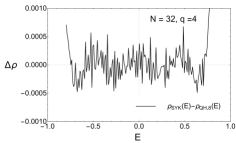
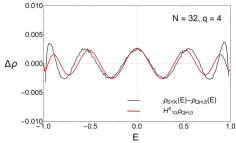
Figure 1: Difference of the of the ensemble average of the spectral density of the SYK Hamiltonian and the eighth order Q-Hermite approximation (black curve). In the left figure, the coefficients are calculated by minimization, and in the right figure by calculating scalar products. The red curve in the right figure is a fit of the contribution of the tenth order Q-Hermite polynomial.

The expansion coefficients can be calculated in two ways. First, from the scalar product of the numerically calculated average spectral density and the Q-Hermite orthogonal polynomials, and second, from minimizing the $L_{2}$ norm of the difference between the numerical result and the expansion up to a given order. The two should give the same results. However, an expansion in orthogonal polynomials does not converge well near the end points of the spectrum, and a much better fit is obtained by excluding a small fraction of the spectrum in this region. In that case, the coefficients cannot be obtained by taking scalar products, but they still can be obtained by minimization. We illustrate this in figure 1 for the average spectral density of an ensemble of 400 SYK Hamiltonians for $N=32$ and $q=4$. What is plotted is the difference of the average spectral density and the eighth order Q-Hermite approximation. In the right figure the coefficients are obtained by calculating the scalar products and the difference (black curve) is close to the contribution of the tenth order Q-Hermite polynomial (red curve). In the left figure, the coefficients are obtained by minimization of $\chi^{2}$ value of the difference not taking into account 2.5% of the total number of eigenvalues at each end of the spectrum. This gives a fit that is a factor 10 better with an accuracy of 1 part in 10000.

We can also expand the spectral density of the SYK Hamiltonian for each configuration in terms of Q-Hermite polynomials

$$\rho_{\rm SYK}(x)=\rho_{\rm QH}(x)\left[1+\sum_{k=1}^{\infty}c_{k}H^{\eta}_{k}\left(x\right)\right].$$ (18)

Now, the $c_{k}$ are stochastic variables whose averages give the expansion coefficients $\langle c_{k}\rangle$ of the average spectral density in equation (12). The fluctuations of $c_{k}$ correspond to spectral fluctuations with wavelength scale of $E_{0}/k$. We expect that these fluctuations are non-universal for small values of $k$, but for large values of $k$, they will correspond to universal random matrix correlations. The aim of this paper is to study at which scale this transition to universal random matrix behavior takes place.

Since the coefficients $c_{k}$ are determined by ${N\choose q}$ independent stochastic variables, the relative error of the $c_{k}$ as well as of $\rho(x)$ is of order $1/{N\choose q}^{1/2}$. We thus expect that the variance of the number of levels in an interval containing $\bar{n}$ levels on average behaves as

$$\Sigma^{2}(\bar{n})\sim\bar{n}^{2}{N\choose q}^{-1}$$ (19)

in agreement with the explicit calculation of $\langle\textrm{Tr}H^{2}\textrm{Tr}H^{2}\rangle$ for the SYK model Altland-ml-2017eao ; Gharibyan-ml-2018jrp . The covariance matrix $\langle c_{k}c_{l}\rangle$ can be calculated analytically for small values for $k$ and $l$ by calculation double-trace moments using methods similar to those first introduced for the calculation of the single-trace moments mon1975 ; Garcia-Garcia-ml-2018kvh ; Berkooz-ml-2018qkz ; Berkooz-ml-2018jqr , see section 6.

4 Collective fluctuations of eigenvalues

As was noticed in earlier work, the main contribution to the number variances comes from overall rescaling of the eigenvalues from one configuration to the next French1973 ; Flores_2001 ; Altland-ml-2017eao ; Garcia-Garcia-ml-2018ruf ; Gharibyan-ml-2018jrp . Such fluctuations can be written as

$$x_{n}\to x_{n}(1+\xi)$$ (20)

where $\xi$ is a stochastic variable with a zero average and a finite variance. The corresponding spectral density fluctuates as

$$\rho(x)=\sum_{k}\delta(x-x_{k}(1+\xi))=\sum_{k}\frac{1}{1+\xi}\delta(\frac{x}{1+\xi}-x_{k})\approx\frac{1}{1+\xi}\overline{\rho}\left(\frac{x}{1+\xi}\right),$$ (21)

where $\overline{\rho}$ is the ensemble-averaged spectral density function so that $\overline{\rho}(z)=\langle\rho(z)\rangle$. This results in a contribution to the two-point correlation function

$$\langle\rho_{2}(x,y)\rangle=\langle\rho(x)\rho(y)\rangle-\langle\rho(x)\rangle\langle\rho(y)\rangle=\langle\xi^{2}\rangle\langle\rho(x)\rangle\langle\rho(y)\rangle+O(\xi^{4}),$$ (22)

where $\langle\xi^{2}\rangle$ denotes averaging over the square of the stochastic variable $\xi$. Since we consider spectral correlations on a scale $|x-y|\ll 1$, terms involving the first and second derivative of $\rho(x)$ can be ignored. The expectation value of $\xi^{2}$ can be obtained from the normalized (by Hilbert space dimension) and rescaled (by variance) double-trace moment $\tilde{M}_{2,2}$, with $\tilde{M}_{m,n}$ defined as

$$\tilde{M}_{m,n}:=\frac{\langle\textrm{Tr}H^{m}\textrm{Tr}H^{n}\rangle}{2^{N}\sigma^{m+n}},$$ (23)

where $\sigma$ is given by (5). As a special case we introduce the notation for (normalized and rescaled) single-trace moments

$$\tilde{M}_{n}:=\tilde{M}_{0,n}.$$ (24)

The $\tilde{M}_{2,2}$ in terms of scale fluctuations is given by

$$\tilde{M}_{2,2}-\tilde{M}_{2}^{2} \approx\int dxdy\left[\left\langle\frac{x^{2}y^{2}}{(1+\xi)^{2}}\overline{\rho}\left(\!\frac{x}{1+\xi}\right)\overline{\rho}\left(\!\frac{y}{1+\xi}\right)\!\right\rangle-\left\langle\frac{x^{2}}{1+\xi}\overline{\rho}\left(\!\frac{x}{1+\xi}\right)\!\right\rangle\left\langle\frac{y^{2}}{1+\xi}\overline{\rho}\left(\!\frac{y}{1+\xi}\right)\!\right\rangle\right]$$

$$\approx\left\langle(1+\xi)^{4}\right\rangle-\left\langle(1+\xi)^{2}\right\rangle^{2}$$

$$\approx 4\left\langle\xi^{2}\right\rangle.$$ (25)

On the other hand, this quantity can be calculated directly in the SYK model Gharibyan-ml-2018jrp :

$$\tilde{M}_{2,2}-\tilde{M}_{2}^{2}=2{N\choose q}^{-1}.$$ (26)

We thus find

$$\langle\xi^{2}\rangle=\frac{1}{2}{N\choose q}^{-1}.$$ (27)

This results in the number variance

$$\Sigma^{2}(\bar{n}) =\int_{x-\Delta/2}^{x+\Delta/2}\int_{x-\Delta/2}^{x+\Delta/2}\langle\xi^{2}\rangle\langle\rho(y)\rangle\langle\rho(z)\rangle dydz$$

$$=\langle\xi^{2}\rangle\bar{n}^{2}$$ (28)

with the average number of levels in the interval given by

$$\bar{n}=\int_{x-\Delta/2}^{x+\Delta/2}dy\langle\rho(y)\rangle.$$ (29)

We can also calculate the contribution of scale fluctuations to arbitrary double-trace moments:

$$\tilde{M}_{2m,2n}-\tilde{M}_{2m}\tilde{M}_{2n}\approx 2mn{N\choose q}^{-1}\tilde{M}_{2m}\tilde{M}_{2n}$$ (30)

This follows from the elementary calculation

$$\tilde{M}_{2m,2n}-\tilde{M}_{2m}\tilde{M}_{2n} \approx\left[\langle(1+\xi)^{2m}(1+\xi)^{2n}\rangle-\langle(1+\xi)^{2m}\rangle\langle(1+\xi)^{2n}\rangle\right]\tilde{M}_{2m}\tilde{M}_{2n}$$

$$\approx 4mn\langle\xi^{2}\rangle\tilde{M}_{2m}\tilde{M}_{2n}$$

$$=2mn{N\choose q}^{-1}\tilde{M}_{2m}\tilde{M}_{2n}.$$ (31)

We will see below that in the SYK model, this result is equal to the average double-trace moment with two cross contractions, see equation (107).

5 Nonlinear $\sigma$-model

Using standard random matrix techniques it is possible to derive a nonlinear $\sigma$-model for the SYK model. For the complex SYK model this was done already in the early eighties Verbaarschot1984 but because of the coupling between the massive and massless modes, it was hard to analyze the $\sigma$-model reliably. The SYK model with Majorana fermions is simpler and Altland and Bagrets obtained Altland-ml-2017eao the following nonlinear $\sigma$-model for the $\beta=2$ universality class (see appendix A for a derivation),

$$Z=\int Da_{\mu}e^{-\frac{1}{2}\sum{}^{{}^{\prime}}_{\mu}T_{\mu}^{-1}{\rm tr}a_{\mu}^{2}-{\rm Tr}\log\left(z+\frac{\sigma}{\sqrt{D}}\sum{}^{{}^{\prime}}_{\mu}a_{\mu}X^{U}_{\mu}\right)}.$$ (32)

The coefficient of $a_{\mu}^{2}$ is not positive definite, but the integrals can be made convergent by an appropriate rotation of the integration contour in the complex plane Altland-ml-2017eao . However, we evaluate the integral perturbatively in a loop expansion about its saddle point when the choice of the integration contour is irrelevant. The $X_{\mu}$’s are all the linearly independent products of Dirac matrices in $N$ dimensions and they form a basis for the vector space of all $2^{N/2}\times 2^{N/2}$ matrices. Because the Hamiltonian commutes with the Dirac chirality matrix $\gamma_{c}$, the Hamiltonian splits into two blocks, and the partition function is for one of the two blocks. Therefore, the sum over $\mu$ is, as indicated by the prime, over the upper block of the $X_{\mu}$ with even $|\mu|$ (the length of the multi-index $\mu$), and only ranges from $0\leq|\mu|\leq N/2$ (with only half the generators for $|\mu|=N/2$, see appendix A). We use the normalization convention that $X_{\mu}^{2}=1$ and denote the upper block by $X_{\mu}^{U}$. As an example, for $N=4$ we have

$$\begin{split}|\mu|=0:\{X_{\mu}\}&=\{\mathbb{1}\},\\ |\mu|=1:\{X_{\mu}\}&=\{\gamma_{i}|i=1,2,3,4\},\\ |\mu|=2:\{X_{\mu}\}&=\{i\gamma_{i_{1}}\gamma_{i_{2}}|1\leq i_{1}<i_{2}\leq 4\},\\ |\mu|=3:\{X_{\mu}\}&=\{i\gamma_{i_{1}}\gamma_{i_{2}}\gamma_{i_{3}}|1\leq i_{1}<i_{2}<i_{3}\leq 4\},\\ |\mu|=4:\{X_{\mu}\}&=\{\gamma_{1}\gamma_{2}\gamma_{3}\gamma_{4}\},\end{split}$$

and in this case the $\sum{}^{{}^{\prime}}_{\mu}$ would be a sum over the set $\{\mathbb{1},i\gamma_{1}\gamma_{2},i\gamma_{1}\gamma_{3},i\gamma_{1}\gamma_{4}\}$. In the analytical calculation we sum over all $\mu$ and correct for that by including the appropriate combinatorial factor. Note that contrary to Altland-ml-2017eao we use Hermitian generators ${X_{\mu}}^{\dagger}=X_{\mu}$. The matrix $a_{\mu}$ is an $2n\times 2n$ matrix in replica space and

$$z=(\underbrace{x+i\epsilon,\cdots,x+i\epsilon}_{n},\underbrace{y-i\epsilon,\cdots,y-i\epsilon}_{n}).$$ (33)

The matrix block corresponding to $x$ or $y$ will be denoted by $11$ or $22$, respectively. The trace over the $2n$-dimensional replica space ($n$-dimensional in case of the one-point function) is denoted by ${\rm tr}$, while the combined trace over the Clifford algebra and the replica space is denoted by Tr. The coefficient $T_{\mu}$ is a combinatorial factor due to the commutation of the $\gamma$ matrices:

$$T_{\mu}=\frac{1}{{N\choose q}}\sum_{j=0}^{q}(-1)^{j}{|\mu|\choose j}{N-|\mu|\choose q-j}$$ (34)

with $|\mu|$ the cardinality of index set $\mu$. It is a Fierz coefficient of the Fierz transformation that arises in the derivation of the $\sigma$-model, see appendix A:

$$T_{\mu}=\frac{1}{D}{N\choose q}^{-1}\sum_{\alpha}\textrm{Tr}\,X^{U}_{\mu}\Gamma^{U}_{\alpha}X^{U}_{\mu}\Gamma^{U}_{\alpha}=2^{-\frac{N}{2}}{N\choose q}^{-1}\sum_{\alpha}\textrm{Tr}\,X_{\mu}\Gamma_{\alpha}X_{\mu}\Gamma_{\alpha}$$ (35)

with $\Gamma_{\alpha}$ the $q$-body operator defined in equation (3) and $D=2^{N/2}/2$.

The pair correlation function is given by

$$C(x,y) =\lim_{n\to 0}\frac{1}{n^{2}}\frac{1}{D^{2}}\frac{d}{dx}\frac{d}{dy}Z(x,y)$$

$$=\lim_{n\to 0}\frac{1}{n^{2}}\frac{1}{D}\frac{1}{\sigma^{2}}\left\langle{\rm tr}P_{11}a_{0}\;{\rm tr}P_{22}a_{0}\right\rangle,$$ (36)

where $P_{pp}$ are the projections onto the $11$ block and $22$ block for $p=1$ and $p=2$, respectively. To obtain this expression we have written the derivatives with respect to $x$ and $y$ as a derivative with respect to $a_{0}$.

The generating function for the one-point function has the same form as in the case of the two-point function, (32), but now $a_{\mu}$ is an $n\times n$ matrix and $z=\text{diag}(\underbrace{x,\cdots,x}_{n})$. The resolvent is given by

$$G(z) =-\frac{1}{n}\frac{1}{D}\textrm{Tr}\frac{d}{dz}\log Z$$

$$=-\lim_{n\to 0}\frac{1}{n}\frac{1}{\sigma\sqrt{D}}\left\langle{\rm tr}\;a_{0}\right\rangle,$$ (37)

where the right-hand side is obtained after a partial integration by expressing the $z$-derivative as a derivative with respect to $a_{0}$.

The aim of this section is to show that the $\sigma$ model (32) reduces to the universal $\sigma$ model of the Gaussian Unitary Ensemble which is given in appendix C.2. The model (32) spontaneouls breaks the ${\rm U}(n,n)$ symmetry of the replica space of the advanced and retarded sectors to ${\rm U}(n)\times{\rm U}(n)$. Because of that we know that the low energy effective Lagrangian is based on this pattern of spontaneous symmetry breaking and is given by the one of the GUE. However, this argument does not determine the prefactor of this universal term, and neither do we know the effect of the coupling between the Goldstone modes and massive modes. As was already realized in 1984 Verbaarschot1984 , these couplings give large corrections which ultimately should cancel in order to arrive at the universal GUE result. However, to this date it has not been shown that such cancellations indeed do happen. The goal of this paper is more modest. We show by a perturbative calculation that the $\sigma$ model (32) gives rise to long range eigenvalue correlations scaling as $1/(x-y)^{2}$, as in case of the GUE, and are consistent with low order moments which can be calculated independently. We also address, the issue, that for the $q=2$ case, which is integrable and should have Poisson statistics, the corrections terms should nullify the universal term. Also in this case we were not able to solve this problem, but we do find a significant quantitative difference between the spectral correlator for $q=2$ and $q=4$.

5.1 One-point function

To better understand the convergence properties of the nonlinear sigma model, it is instructive to work out the one-point function. The generating function for the one-point function has the same form as in the case of the two-point function, (32), but now $a_{\mu}$ is an $n\times n$ matrix and $z=(\underbrace{x,\cdots,x}_{n})$. The resolvent is given by

$$G(z)=\int Da_{\mu}\frac{\sqrt{D}}{\sigma}(-a_{0})e^{-\frac{1}{2}\sum{}^{{}^{\prime}}_{\mu}T_{\mu}^{-1}{\rm tr}a_{\mu}^{2}-{\rm Tr}\log\left(z+\frac{\sigma}{\sqrt{D}}\sum{}^{{}^{\prime}}_{\mu}a_{\mu}X^{U}_{\mu}\right)},$$ (38)

where $a_{0}$ is the diagonal element of the replica matrix. We evaluate the integral by a loop expansion about the saddle point. The saddle point equation is given by

$$T_{\mu}^{-1}a_{\mu}+\textrm{Tr}\frac{\sigma X^{U}_{\mu}/\sqrt{D}}{z+\sigma\sum{}^{{}^{\prime}}_{\mu}X^{U}_{\mu}a_{\mu}/\sqrt{D}}=0,$$ (39)

where the trace Tr is over the gamma matrices. By inspection one realizes that a solution is given by Verbaarschot1984

$$a_{\mu}=\bar{a}\delta_{\mu 0},$$ (40)

with

$$\bar{a}+\frac{\sigma\sqrt{D}}{z+\sigma\bar{a}/\sqrt{D}}=0.$$ (41)

For $\mu\neq 0$ this follows from the fact that $\textrm{Tr}X^{U}_{\mu}=0$. The saddle point result for the resolvent is equal to

$$\bar{G}(z)=-\frac{\bar{a}}{\sigma\sqrt{D}}.$$ (42)

The resolvent thus satisfies the saddle point equation

$$\bar{G}+\frac{1}{z+\sigma^{2}\bar{G}}=0,$$ (43)

and is given by

$$\bar{G}=\frac{z}{2\sigma^{2}}-\frac{1}{2\sigma^{2}}\sqrt{z^{2}-4\sigma^{2}}.$$ (44)

We expand $a_{\mu}$ about its saddle point

$$a_{\mu}=\bar{a}+\alpha_{\mu}.$$ (45)

Using the saddle point equation for $\overline{a}$, we expand the logarithm as

$$-\textrm{Tr}\log(z+\frac{\sigma}{\sqrt{D}}\sum_{\mu}{}^{{}^{\prime}}a_{\mu}X^{U}_{\mu}) =\textrm{Tr}\sum_{k=1}^{\infty}\frac{1}{k}\left(\frac{\bar{a}}{D}\sum{}^{{}^{\prime}}_{\mu}\alpha_{\mu}X^{U}_{\mu}\right)^{k}$$ (46)

$$=\textrm{Tr}\sum_{k=1}^{\infty}\frac{1}{k}\left(\frac{-\bar{G}\sigma}{\sqrt{D}}\sum{}^{{}^{\prime}}_{\mu}\alpha_{\mu}X^{U}_{\mu}\right)^{k}.$$ (47)

This results in the propagator

$$\langle\alpha_{\mu}^{kl}\alpha_{\nu}^{mn}\rangle=\delta_{\mu\nu}\delta_{lm}\delta_{kn}\frac{T_{\mu}}{1-T_{\mu}\left(\;{\bar{G}\sigma}\right)^{2}},$$ (48)

while the vertices of the loop expansion are given by

$$\textrm{Tr}\sum_{k=3}^{\infty}\frac{1}{k}\left(\frac{-\bar{G}\sigma}{\sqrt{D}}\sum_{\mu}{}^{{}^{\prime}}\alpha_{\mu}X^{U}_{\mu}\right)^{k}.$$ (49)

We now calculate the resolvent to two-loop order in this expansion. The one-loop contribution, $\langle\textrm{Tr}a_{0}\textrm{Tr}(\sum{}^{{}^{\prime}}_{\mu}\alpha_{\mu}X^{U}_{\mu})^{3}\rangle$, vanishes in the replica limit. The first nonvanishing contribution, $\langle\textrm{Tr}a_{0}\textrm{Tr}(\sum{}^{{}^{\prime}}_{\mu}\alpha_{\mu}X^{U}_{\mu})^{5}\rangle$, is given by the diagram

$$\mathchoice{\vbox{\hbox to0.0pt{\kern 9.4722pt\kern 3.1985pt\hbox{\vrule width=0.50003pt,height=0.0pt,depth=4.30554pt\vrule width=17.53584pt,height=0.0pt,depth=0.50003pt\vrule width=0.50003pt,height=0.0pt,depth=4.30554pt}\hss}\vskip 2.15277pt\vskip 4.30554pt}}{\vbox{\hbox to0.0pt{\kern 9.4722pt\kern 3.1985pt\hbox{\vrule width=0.50003pt,height=0.0pt,depth=4.30554pt\vrule width=17.53584pt,height=0.0pt,depth=0.50003pt\vrule width=0.50003pt,height=0.0pt,depth=4.30554pt}\hss}\vskip 2.15277pt\vskip 4.30554pt}}{\vbox{\hbox to0.0pt{\kern 7.13052pt\kern 2.23895pt\hbox{\vrule width=0.50003pt,height=0.0pt,depth=4.30554pt\vrule width=13.27505pt,height=0.0pt,depth=0.50003pt\vrule width=0.50003pt,height=0.0pt,depth=4.30554pt}\hss}\vskip 2.15277pt\vskip 3.01389pt}}{\vbox{\hbox to0.0pt{\kern 5.5694pt\kern 1.59924pt\hbox{\vrule width=0.50003pt,height=0.0pt,depth=4.30554pt\vrule width=10.43452pt,height=0.0pt,depth=0.50003pt\vrule width=0.50003pt,height=0.0pt,depth=4.30554pt}\hss}\vskip 2.15277pt\vskip 2.15277pt}}\mathchoice{\vbox{\hbox to0.0pt{\kern 33.40506pt\kern 3.1985pt\hbox{\vrule width=0.50003pt,height=0.0pt,depth=8.61108pt\vrule width=12.79404pt,height=0.0pt,depth=0.50003pt\vrule width=0.50003pt,height=0.0pt,depth=8.61108pt}\hss}\vskip 2.15277pt\vskip 4.30554pt}}{\vbox{\hbox to0.0pt{\kern 33.40506pt\kern 3.1985pt\hbox{\vrule width=0.50003pt,height=0.0pt,depth=8.61108pt\vrule width=12.79404pt,height=0.0pt,depth=0.50003pt\vrule width=0.50003pt,height=0.0pt,depth=8.61108pt}\hss}\vskip 2.15277pt\vskip 4.30554pt}}{\vbox{\hbox to0.0pt{\kern 24.88348pt\kern 2.23895pt\hbox{\vrule width=0.50003pt,height=0.0pt,depth=8.61108pt\vrule width=8.95581pt,height=0.0pt,depth=0.50003pt\vrule width=0.50003pt,height=0.0pt,depth=8.61108pt}\hss}\vskip 2.15277pt\vskip 3.01389pt}}{\vbox{\hbox to0.0pt{\kern 19.20242pt\kern 1.59924pt\hbox{\vrule width=0.50003pt,height=0.0pt,depth=8.61108pt\vrule width=6.397pt,height=0.0pt,depth=0.50003pt\vrule width=0.50003pt,height=0.0pt,depth=8.61108pt}\hss}\vskip 2.15277pt\vskip 2.15277pt}}\mathchoice{\vbox{\hbox to0.0pt{\kern 39.80208pt\kern 3.1985pt\hbox{\vrule width=0.50003pt,height=0.0pt,depth=12.91663pt\vrule width=12.79404pt,height=0.0pt,depth=0.50003pt\vrule width=0.50003pt,height=0.0pt,depth=12.91663pt}\hss}\vskip 2.15277pt\vskip 4.30554pt}}{\vbox{\hbox to0.0pt{\kern 39.80208pt\kern 3.1985pt\hbox{\vrule width=0.50003pt,height=0.0pt,depth=12.91663pt\vrule width=12.79404pt,height=0.0pt,depth=0.50003pt\vrule width=0.50003pt,height=0.0pt,depth=12.91663pt}\hss}\vskip 2.15277pt\vskip 4.30554pt}}{\vbox{\hbox to0.0pt{\kern 29.36139pt\kern 2.23895pt\hbox{\vrule width=0.50003pt,height=0.0pt,depth=12.91663pt\vrule width=8.95581pt,height=0.0pt,depth=0.50003pt\vrule width=0.50003pt,height=0.0pt,depth=12.91663pt}\hss}\vskip 2.15277pt\vskip 3.01389pt}}{\vbox{\hbox to0.0pt{\kern 22.40092pt\kern 1.59924pt\hbox{\vrule width=0.50003pt,height=0.0pt,depth=12.91663pt\vrule width=6.397pt,height=0.0pt,depth=0.50003pt\vrule width=0.50003pt,height=0.0pt,depth=12.91663pt}\hss}\vskip 2.15277pt\vskip 2.15277pt}}{\rm tr}\,\alpha\,{\rm tr}\,\alpha\alpha\alpha\alpha\alpha.$$ (50)

Writing out the indices and the traces over the replica space we obtain

(51)

From the progator (48) it is immediately clear that the only nonvanishing contractions are those with replica indices $k=l$. Since the propagtor is replica symmetric, the sum over $k$ gives an overall factor $n$ which is cancelled by the $1/n$ factor of the replica limit (37). Combining this with the factors $X_{\mu}^{U}$ we obtain

$$\sum_{\mu}{}^{{}^{\prime}}\sum_{\nu}{}^{{}^{\prime}}\frac{\bar{G}^{5}\sigma^{4}}{D^{2}(1-\bar{G}^{2})}\frac{T_{\mu}}{1-T_{\mu}\left({\bar{G}\sigma}\right)^{2}}\frac{T_{\nu}}{1-T_{\nu}\left(\bar{G}\sigma\right)^{2}}\frac{1}{D}\textrm{Tr}X^{U}_{\mu}X^{U}_{\nu}X^{U}_{\mu}X^{U}_{\nu}.$$ (52)

The trace can be evaluated by observing that $X^{U}_{\mu}$ and $X^{U}_{\nu}$ commute or anti-commute depending on the number of gamma matrices they have in common, while $T_{\mu}$ only depends on the number of indices in $\mu$. This results in

$$\sum_{m}{}^{{}^{\prime}}\sum_{n}{}^{{}^{\prime}}{N\choose m}\frac{\bar{G}^{5}\sigma^{4}}{D^{2}(1-\bar{G}^{2})}\frac{T_{m}}{1-T_{m}\left({\bar{G}\sigma}\right)^{2}}\frac{T_{n}}{1-T_{n}\left(\bar{G}\sigma\right)^{2}}\sum_{p=0}^{m}(-1)^{p}{m\choose p}{N-m\choose n-p}$$

$$=\frac{\sigma^{4}\eta}{z^{5}}+\frac{\sigma^{6}(6\eta+2\eta^{2})}{z^{7}}+O(1/z^{9}).$$ (53)

The coefficients of the $1/z$ expansion can be obtained by using various combinatorial identities, see appendix B. The normalized fourth moment is thus given by

$$\frac{M_{4}}{\sigma^{4}}=2+\eta.$$ (54)

Next we consider the contribution

$$\lim_{n\to 0}\frac{1}{n}\frac{1}{D}\left\langle\frac{1}{12}\bar{G}(z){\rm tr}\alpha_{0}{\textrm{Tr}}\left(\frac{\bar{G}(z)\sigma}{\sqrt{D}}\sum_{\mu}{}^{{}^{\prime}}\alpha_{\mu}X^{U}_{\mu}\right)^{3}{\textrm{Tr}}\left(\frac{\bar{G}(z)\sigma}{\sqrt{D}}\sum_{\mu}{}^{{}^{\prime}}\alpha_{\mu}X^{U}_{\mu}\right)^{4}\right\rangle,$$ (55)

which permits two different contraction patterns. For the diagram

$$\mathchoice{\vbox{\hbox to0.0pt{\kern 9.4722pt\kern 3.1985pt\hbox{\vrule width=0.50003pt,height=0.0pt,depth=4.30554pt\vrule width=47.86572pt,height=0.0pt,depth=0.50003pt\vrule width=0.50003pt,height=0.0pt,depth=4.30554pt}\hss}\vskip 2.15277pt\vskip 4.30554pt}}{\vbox{\hbox to0.0pt{\kern 9.4722pt\kern 3.1985pt\hbox{\vrule width=0.50003pt,height=0.0pt,depth=4.30554pt\vrule width=47.86572pt,height=0.0pt,depth=0.50003pt\vrule width=0.50003pt,height=0.0pt,depth=4.30554pt}\hss}\vskip 2.15277pt\vskip 4.30554pt}}{\vbox{\hbox to0.0pt{\kern 7.13052pt\kern 2.23895pt\hbox{\vrule width=0.50003pt,height=0.0pt,depth=4.30554pt\vrule width=35.50592pt,height=0.0pt,depth=0.50003pt\vrule width=0.50003pt,height=0.0pt,depth=4.30554pt}\hss}\vskip 2.15277pt\vskip 3.01389pt}}{\vbox{\hbox to0.0pt{\kern 5.5694pt\kern 1.59924pt\hbox{\vrule width=0.50003pt,height=0.0pt,depth=4.30554pt\vrule width=27.26605pt,height=0.0pt,depth=0.50003pt\vrule width=0.50003pt,height=0.0pt,depth=4.30554pt}\hss}\vskip 2.15277pt\vskip 2.15277pt}}\mathchoice{\vbox{\hbox to0.0pt{\kern 27.00804pt\kern 3.1985pt\hbox{\vrule width=0.50003pt,height=0.0pt,depth=8.61108pt\vrule width=36.7269pt,height=0.0pt,depth=0.50003pt\vrule width=0.50003pt,height=0.0pt,depth=8.61108pt}\hss}\vskip 2.15277pt\vskip 4.30554pt}}{\vbox{\hbox to0.0pt{\kern 27.00804pt\kern 3.1985pt\hbox{\vrule width=0.50003pt,height=0.0pt,depth=8.61108pt\vrule width=36.7269pt,height=0.0pt,depth=0.50003pt\vrule width=0.50003pt,height=0.0pt,depth=8.61108pt}\hss}\vskip 2.15277pt\vskip 4.30554pt}}{\vbox{\hbox to0.0pt{\kern 20.40558pt\kern 2.23895pt\hbox{\vrule width=0.50003pt,height=0.0pt,depth=8.61108pt\vrule width=26.70877pt,height=0.0pt,depth=0.50003pt\vrule width=0.50003pt,height=0.0pt,depth=8.61108pt}\hss}\vskip 2.15277pt\vskip 3.01389pt}}{\vbox{\hbox to0.0pt{\kern 16.00392pt\kern 1.59924pt\hbox{\vrule width=0.50003pt,height=0.0pt,depth=8.61108pt\vrule width=20.03003pt,height=0.0pt,depth=0.50003pt\vrule width=0.50003pt,height=0.0pt,depth=8.61108pt}\hss}\vskip 2.15277pt\vskip 2.15277pt}}\mathchoice{\vbox{\hbox to0.0pt{\kern 33.40506pt\kern 3.1985pt\hbox{\vrule width=0.50003pt,height=0.0pt,depth=12.91663pt\vrule width=36.7269pt,height=0.0pt,depth=0.50003pt\vrule width=0.50003pt,height=0.0pt,depth=12.91663pt}\hss}\vskip 2.15277pt\vskip 4.30554pt}}{\vbox{\hbox to0.0pt{\kern 33.40506pt\kern 3.1985pt\hbox{\vrule width=0.50003pt,height=0.0pt,depth=12.91663pt\vrule width=36.7269pt,height=0.0pt,depth=0.50003pt\vrule width=0.50003pt,height=0.0pt,depth=12.91663pt}\hss}\vskip 2.15277pt\vskip 4.30554pt}}{\vbox{\hbox to0.0pt{\kern 24.88348pt\kern 2.23895pt\hbox{\vrule width=0.50003pt,height=0.0pt,depth=12.91663pt\vrule width=26.70877pt,height=0.0pt,depth=0.50003pt\vrule width=0.50003pt,height=0.0pt,depth=12.91663pt}\hss}\vskip 2.15277pt\vskip 3.01389pt}}{\vbox{\hbox to0.0pt{\kern 19.20242pt\kern 1.59924pt\hbox{\vrule width=0.50003pt,height=0.0pt,depth=12.91663pt\vrule width=20.03003pt,height=0.0pt,depth=0.50003pt\vrule width=0.50003pt,height=0.0pt,depth=12.91663pt}\hss}\vskip 2.15277pt\vskip 2.15277pt}}\mathchoice{\vbox{\hbox to0.0pt{\kern 39.80208pt\kern 3.1985pt\hbox{\vrule width=0.50003pt,height=0.0pt,depth=17.22217pt\vrule width=36.7269pt,height=0.0pt,depth=0.50003pt\vrule width=0.50003pt,height=0.0pt,depth=17.22217pt}\hss}\vskip 2.15277pt\vskip 4.30554pt}}{\vbox{\hbox to0.0pt{\kern 39.80208pt\kern 3.1985pt\hbox{\vrule width=0.50003pt,height=0.0pt,depth=17.22217pt\vrule width=36.7269pt,height=0.0pt,depth=0.50003pt\vrule width=0.50003pt,height=0.0pt,depth=17.22217pt}\hss}\vskip 2.15277pt\vskip 4.30554pt}}{\vbox{\hbox to0.0pt{\kern 29.36139pt\kern 2.23895pt\hbox{\vrule width=0.50003pt,height=0.0pt,depth=17.22217pt\vrule width=26.70877pt,height=0.0pt,depth=0.50003pt\vrule width=0.50003pt,height=0.0pt,depth=17.22217pt}\hss}\vskip 2.15277pt\vskip 3.01389pt}}{\vbox{\hbox to0.0pt{\kern 22.40092pt\kern 1.59924pt\hbox{\vrule width=0.50003pt,height=0.0pt,depth=17.22217pt\vrule width=20.03003pt,height=0.0pt,depth=0.50003pt\vrule width=0.50003pt,height=0.0pt,depth=17.22217pt}\hss}\vskip 2.15277pt\vskip 2.15277pt}}{\rm tr}\,\alpha\,{\rm tr}\,\alpha\alpha\alpha\,{\rm tr}\,\alpha\alpha\alpha\alpha$$ (56)

we find after taking the replica limit

$$\frac{1}{D^{4}}\frac{\bar{G}^{7}\sigma^{6}}{1-\sigma^{2}\bar{G}^{2}}\sum_{\mu\nu\rho}{}^{{}^{\prime}}\frac{T_{\mu}}{1-T_{\mu}\left({\bar{G}\sigma}\right)^{2}}\frac{T_{\nu}}{1-T_{\nu}\left({\bar{G}\sigma}\right)^{2}}\frac{T_{\rho}}{1-T_{\rho}\left({\bar{G}\sigma}\right)^{2}}\textrm{Tr}X^{U}_{\mu}X^{U}_{\nu}X^{U}_{\rho}\textrm{Tr}X^{U}_{\mu}X^{U}_{\nu}X^{U}_{\rho}.$$ (57)

The traces are only nonzero if $X^{U}_{\rho}$ contains the gamma matrices that $X^{U}_{\mu}$ and $X^{U}_{\nu}$ do not have in common. For $m_{1}$ gamma matrices in $X^{U}_{\mu}$, $m_{2}$ gamma matrices in $X^{U}_{\nu}$ and $s$ common gamma matrices this gives the combinatorial factor

$$D^{2}{N\choose m_{1}}{m_{1}\choose s}{N-m_{1}\choose m_{2}-s}(-1)^{s},$$ (58)

where the phase factor is due to the fact that only $i^{s}X^{U}_{\mu}X^{U}_{\nu}$ is Hermitian. The diagram (57) is thus equal to

$$\frac{1}{D^{2}}\frac{\bar{G}^{7}\sigma^{6}}{1-\sigma^{2}\bar{G}^{2}}\frac{1}{4}\sum_{m_{1}=0}^{N}\sum_{m_{2}=0}^{N}\sum_{s=0}^{m_{1}}\frac{T_{m_{1}}}{1-T_{m_{1}}\left({\bar{G}\sigma}\right)^{2}}\frac{T_{m_{2}}}{1-T_{m_{2}}\left({\bar{G}\sigma}\right)^{2}}\frac{T_{m_{1}+m_{2}-2s}}{1-T_{m_{1}+m_{2}-2s}\left({\bar{G}\sigma}\right)^{2}}$$

$$\times{N\choose m_{1}}{m_{1}\choose s}{N-m_{1}\choose m_{2}-s}(-1)^{s}.$$ (59)

The sums for the leading order term in the $1/z$ expansion of the resolvent can be evaluated as the contribution $T_{6}$ Garcia-Garcia-ml-2018kvh , see appendix B. The combinatorial factor $1/4$ is to account for the prime on the sums in equation (57). Note that the sum over $m_{1}$ and $m_{2}$ only runs up to $N/2$ while the sum over odd $m_{1}$ and $m_{2}$ vanishes anyway. We thus obtain the large $z$ expansion of the correction

$$\frac{T_{6}}{z^{7}}+O(1/z^{9}).$$ (60)

The second diagram

$$\mathchoice{\vbox{\hbox to0.0pt{\kern 9.4722pt\kern 3.1985pt\hbox{\vrule width=0.50003pt,height=0.0pt,depth=4.30554pt\vrule width=17.53584pt,height=0.0pt,depth=0.50003pt\vrule width=0.50003pt,height=0.0pt,depth=4.30554pt}\hss}\vskip 2.15277pt\vskip 4.30554pt}}{\vbox{\hbox to0.0pt{\kern 9.4722pt\kern 3.1985pt\hbox{\vrule width=0.50003pt,height=0.0pt,depth=4.30554pt\vrule width=17.53584pt,height=0.0pt,depth=0.50003pt\vrule width=0.50003pt,height=0.0pt,depth=4.30554pt}\hss}\vskip 2.15277pt\vskip 4.30554pt}}{\vbox{\hbox to0.0pt{\kern 7.13052pt\kern 2.23895pt\hbox{\vrule width=0.50003pt,height=0.0pt,depth=4.30554pt\vrule width=13.27505pt,height=0.0pt,depth=0.50003pt\vrule width=0.50003pt,height=0.0pt,depth=4.30554pt}\hss}\vskip 2.15277pt\vskip 3.01389pt}}{\vbox{\hbox to0.0pt{\kern 5.5694pt\kern 1.59924pt\hbox{\vrule width=0.50003pt,height=0.0pt,depth=4.30554pt\vrule width=10.43452pt,height=0.0pt,depth=0.50003pt\vrule width=0.50003pt,height=0.0pt,depth=4.30554pt}\hss}\vskip 2.15277pt\vskip 2.15277pt}}\mathchoice{\vbox{\hbox to0.0pt{\kern 33.40506pt\kern 3.1985pt\hbox{\vrule width=0.50003pt,height=0.0pt,depth=8.61108pt\vrule width=23.93286pt,height=0.0pt,depth=0.50003pt\vrule width=0.50003pt,height=0.0pt,depth=8.61108pt}\hss}\vskip 2.15277pt\vskip 4.30554pt}}{\vbox{\hbox to0.0pt{\kern 33.40506pt\kern 3.1985pt\hbox{\vrule width=0.50003pt,height=0.0pt,depth=8.61108pt\vrule width=23.93286pt,height=0.0pt,depth=0.50003pt\vrule width=0.50003pt,height=0.0pt,depth=8.61108pt}\hss}\vskip 2.15277pt\vskip 4.30554pt}}{\vbox{\hbox to0.0pt{\kern 24.88348pt\kern 2.23895pt\hbox{\vrule width=0.50003pt,height=0.0pt,depth=8.61108pt\vrule width=17.75296pt,height=0.0pt,depth=0.50003pt\vrule width=0.50003pt,height=0.0pt,depth=8.61108pt}\hss}\vskip 2.15277pt\vskip 3.01389pt}}{\vbox{\hbox to0.0pt{\kern 19.20242pt\kern 1.59924pt\hbox{\vrule width=0.50003pt,height=0.0pt,depth=8.61108pt\vrule width=13.63303pt,height=0.0pt,depth=0.50003pt\vrule width=0.50003pt,height=0.0pt,depth=8.61108pt}\hss}\vskip 2.15277pt\vskip 2.15277pt}}\mathchoice{\vbox{\hbox to0.0pt{\kern 39.80208pt\kern 3.1985pt\hbox{\vrule width=0.50003pt,height=0.0pt,depth=12.91663pt\vrule width=30.32988pt,height=0.0pt,depth=0.50003pt\vrule width=0.50003pt,height=0.0pt,depth=12.91663pt}\hss}\vskip 2.15277pt\vskip 4.30554pt}}{\vbox{\hbox to0.0pt{\kern 39.80208pt\kern 3.1985pt\hbox{\vrule width=0.50003pt,height=0.0pt,depth=12.91663pt\vrule width=30.32988pt,height=0.0pt,depth=0.50003pt\vrule width=0.50003pt,height=0.0pt,depth=12.91663pt}\hss}\vskip 2.15277pt\vskip 4.30554pt}}{\vbox{\hbox to0.0pt{\kern 29.36139pt\kern 2.23895pt\hbox{\vrule width=0.50003pt,height=0.0pt,depth=12.91663pt\vrule width=22.23087pt,height=0.0pt,depth=0.50003pt\vrule width=0.50003pt,height=0.0pt,depth=12.91663pt}\hss}\vskip 2.15277pt\vskip 3.01389pt}}{\vbox{\hbox to0.0pt{\kern 22.40092pt\kern 1.59924pt\hbox{\vrule width=0.50003pt,height=0.0pt,depth=12.91663pt\vrule width=16.83153pt,height=0.0pt,depth=0.50003pt\vrule width=0.50003pt,height=0.0pt,depth=12.91663pt}\hss}\vskip 2.15277pt\vskip 2.15277pt}}\mathchoice{\vbox{\hbox to0.0pt{\kern 63.73494pt\kern 3.1985pt\hbox{\vrule width=0.50003pt,height=0.0pt,depth=17.22217pt\vrule width=12.79404pt,height=0.0pt,depth=0.50003pt\vrule width=0.50003pt,height=0.0pt,depth=17.22217pt}\hss}\vskip 2.15277pt\vskip 4.30554pt}}{\vbox{\hbox to0.0pt{\kern 63.73494pt\kern 3.1985pt\hbox{\vrule width=0.50003pt,height=0.0pt,depth=17.22217pt\vrule width=12.79404pt,height=0.0pt,depth=0.50003pt\vrule width=0.50003pt,height=0.0pt,depth=17.22217pt}\hss}\vskip 2.15277pt\vskip 4.30554pt}}{\vbox{\hbox to0.0pt{\kern 47.11435pt\kern 2.23895pt\hbox{\vrule width=0.50003pt,height=0.0pt,depth=17.22217pt\vrule width=8.95581pt,height=0.0pt,depth=0.50003pt\vrule width=0.50003pt,height=0.0pt,depth=17.22217pt}\hss}\vskip 2.15277pt\vskip 3.01389pt}}{\vbox{\hbox to0.0pt{\kern 36.03395pt\kern 1.59924pt\hbox{\vrule width=0.50003pt,height=0.0pt,depth=17.22217pt\vrule width=6.397pt,height=0.0pt,depth=0.50003pt\vrule width=0.50003pt,height=0.0pt,depth=17.22217pt}\hss}\vskip 2.15277pt\vskip 2.15277pt}}{\rm tr}\,\alpha\,{\rm tr}\,\alpha\alpha\alpha\,{\rm tr}\,\alpha\alpha\alpha\alpha$$ (61)

is equal to

$$\frac{1}{D^{4}}\frac{\bar{G}^{7}\sigma^{6}}{1-\sigma^{2}\bar{G}^{2}}\sum_{\mu\nu}{}^{{}^{\prime}}\frac{T_{\mu}^{2}}{(1-T_{\mu}\left({\bar{G}\sigma}\right)^{2})^{2}}\frac{T_{\nu}}{1-T_{\nu}\left({\bar{G}\sigma}\right)^{2}}\textrm{Tr}X^{U}_{\mu}X^{U}_{\mu}\textrm{Tr}X^{U}_{\mu}X^{U}_{\nu}X^{U}_{\mu}X^{U}_{\nu}$$

$$=\frac{\sigma^{6}\eta^{2}}{z^{7}}+O(1/z^{9}),$$ (62)

where we have used combinatorial identities to obtain the coefficient of $1/z^{7}$.

To summarize, starting from the generating function $Z$, we have obtained the normalized sixth moment

$$\frac{M_{6}}{\sigma^{6}}=5+6\eta+3\eta^{2}+T_{6}$$ (63)

in agreement with an explicit moment calculation of the SYK model Garcia-Garcia-ml-2016mno .

If we continue this expansion we will recover the full $1/z$ expansion of the resolvent of the SYK model. This expansion is not well behaved for $z$ close to the support of the spectrum and will have to be resummed to obtain nonperturbative results, see section 5.3 for more discussion of this issue.

5.2 Loop expansion of the two-point function

The saddle-point equation for the two-point function has the same form as equation (39) but now $z$ is a vector of length $2n$, see equation (33), and $a_{\mu}$ is a $2n\times 2n$ matrix. The solution with $a_{\mu}^{12}=0$ is the same as for the one-point function with $z$ replaced by $x$ and $y$ for the 11-sector and the 22-sector, respectively,

$$\bar{a}^{11}+\frac{\sigma\sqrt{D}}{x+\sigma\bar{a}^{11}/\sqrt{D}}=0,\qquad\bar{a}^{22}+\frac{\sigma\sqrt{D}}{y+\sigma\bar{a}^{22}/\sqrt{D}}=0.$$ (64)

The saddle point value of the resolvent is thus given by

$$\bar{G}=\left(\begin{array}[]{cc}\bar{G}(x)\mathbb{I}_{n}&0\\ 0&\bar{G}(y)\mathbb{I}_{n}\end{array}\right),$$ (65)

where $\bar{G}(x)$ and $\bar{G}(y)$ are related to $\bar{a}_{11}$ and $\bar{a}_{22}$ according to equation (42), in this order.

The propagator and vertices follow from the expansion of the logarithm in the action

$$-\textrm{Tr}\log(z+\frac{\sigma}{\sqrt{D}}\sum_{\mu}{}^{{}^{\prime}}a_{\mu}X^{U}_{\mu}) =\textrm{Tr}\sum_{k=1}^{\infty}\frac{1}{k}\left(\frac{\bar{a}}{D}\sum_{\mu}{}^{{}^{\prime}}\alpha_{\mu}X^{U}_{\mu}\right)^{k}$$ (66)

$$=\textrm{Tr}\sum_{k=1}^{\infty}\frac{1}{k}\left(\frac{-\bar{G}\sigma}{\sqrt{D}}\sum_{\mu}{}^{{}^{\prime}}\alpha_{\mu}X^{U}_{\mu}\right)^{k}.$$ (67)

The propagator is thus given by

$$\langle\alpha_{\mu}^{pq}\alpha_{\nu}^{qp}\rangle=\delta_{\mu\nu}\frac{T_{\mu}}{1-T_{\mu}\sigma^{2}\bar{G}(x_{p})\bar{G}(x_{q})}.$$ (68)

We first calculate the one-loop contribution to the two-point correlator

$$C(x,y)=\left\langle\frac{1}{n}\frac{1}{D}\frac{\sqrt{D}}{\sigma}{\rm tr}P_{11}\alpha_{0}\frac{1}{n}\frac{1}{D}\frac{\sqrt{D}}{\sigma}{\rm tr}P_{22}\alpha_{0}\right\rangle.$$ (69)

As is the case for the GUE (see appendix C.2) we have two contributions. The first contribution is given by

$$\frac{1}{n}\frac{1}{D}\left\langle\frac{\sqrt{D}}{\sigma}{\rm tr}P_{11}\alpha_{0}\frac{1}{n}\frac{1}{D}\frac{\sqrt{D}}{\sigma}{\rm tr}P_{22}\alpha_{0}\frac{1}{4}\textrm{Tr}\left(\frac{-\bar{G}\sigma}{\sqrt{D}}\sum_{\mu}{}^{{}^{\prime}}\alpha_{\mu}X^{U}_{\mu}\right)^{4}\right\rangle$$

$$=\frac{1}{n^{2}}\frac{1}{D^{3}}\sigma^{2}\bar{G}^{2}(x)\bar{G}^{2}(y)\left\langle{\rm tr}\alpha^{11}_{0}{\rm tr}\alpha^{22}_{0}\sum_{\mu}{}^{{}^{\prime}}\textrm{Tr}\alpha^{11}_{0}\alpha_{\mu}^{12}X^{U}_{\mu}\alpha_{0}^{22}\alpha_{\mu}^{21}X^{U}_{\mu}\right\rangle$$

$$=\frac{\sigma^{2}}{D^{2}}\sum_{\mu}{}^{{}^{\prime}}\frac{\bar{G}^{2}(x)\bar{G}^{2}(y)T_{\mu}}{(1-T_{\mu}\sigma^{2}\bar{G}(x)\bar{G}(y))(1-\sigma^{2}\bar{G}^{2}(x))(1-\sigma^{2}\bar{G}^{2}(y))}$$

$$=\left(\sigma^{4}\frac{1}{x^{3}y^{3}}+2\sigma^{6}\frac{1}{x^{4}y^{4}}\right){N\choose q}^{-1}+\frac{\sigma^{6}}{D^{2}}\frac{1}{x^{4}y^{4}}\sum_{\mu}{}^{{}^{\prime}}T_{\mu}^{3}+\cdots\,$$ (70)

where we have used that

$$\sum_{\mu}{}^{{}^{\prime}}T_{\mu}=0,\qquad\frac{1}{D^{2}}\sum_{\mu}{}^{{}^{\prime}}T_{\mu}^{2}=\frac{1}{D^{2}}\frac{1}{4}\sum_{|\mu|=0}^{N}{N\choose|\mu|}T_{\mu}^{2}={N\choose q}^{-1},$$ (71)

and that the sum over $\mu$ in equation (70), as indicated by the primes, only runs over the even values of $\mu<N/2$ resulting in the combinatorial factor of $1/4$.

The second one-loop contribution to the two-point function is given by

$$\frac{1}{n}\frac{1}{D}\left\langle\frac{\sqrt{D}}{\sigma}{\rm tr}P_{11}\alpha_{0}\frac{1}{n}\frac{1}{D}\frac{\sqrt{D}}{\sigma}{\rm tr}P_{22}\alpha_{0}\frac{1}{18}\textrm{Tr}^{2}\left(\frac{-\bar{G}\sigma}{\sqrt{D}}\sum_{\mu}{}^{{}^{\prime}}\alpha_{\mu}X^{U}_{\mu}\right)^{3}\right\rangle$$

$$=\frac{1}{n^{2}}\frac{1}{D^{4}}\sigma^{4}\bar{G}^{3}(x)\bar{G}^{3}(y)\left\langle{\rm tr}\alpha^{11}_{0}{\rm tr}\alpha^{22}_{0}\sum_{\mu}{}^{{}^{\prime}}\textrm{Tr}\alpha^{11}_{0}\alpha_{\mu}^{12}X^{U}_{\mu}\alpha_{\mu}^{21}X^{U}_{\mu}\sum_{\nu}{}^{{}^{\prime}}\textrm{Tr}\alpha^{22}_{0}\alpha_{\nu}^{21}X^{U}_{\nu}\alpha_{\nu}^{12}X^{U}_{\nu}\right\rangle$$

$$=\frac{\sigma^{4}}{D^{2}}\sum_{\mu}{}^{{}^{\prime}}\frac{\bar{G}^{3}(x)\bar{G}^{3}(y)T_{\mu}^{2}}{(1-T_{\mu}\sigma^{2}\bar{G}(x)\bar{G}(y))^{2}(1-\sigma^{2}\bar{G}^{2}(x))(1-\sigma^{2}\bar{G}^{2}(y))}$$

$$=\left(\sigma^{4}\frac{1}{x^{3}y^{3}}-2\sigma^{6}\frac{1}{x^{4}y^{4}}\right){{N\choose q}}^{-1}+2\frac{\sigma^{6}}{D^{2}}\frac{1}{x^{4}y^{4}}\sum_{\mu}{}^{{}^{\prime}}T_{\mu}^{3}+\cdots\$$ (72)

after taking the replica limit.

The sum of the two contributions is equal to

$$\frac{\sigma^{2}}{D^{2}}\sum_{\mu}{}^{{}^{\prime}}\frac{\bar{G}^{2}(x)\bar{G}^{2}(y)T_{\mu}}{(1-T_{\mu}\sigma^{2}\bar{G}(x)\bar{G}(y))^{2}(1-\sigma^{2}\bar{G}(x)\bar{G}(x))(1-\sigma^{2}\bar{G}(y)\bar{G}(y))}$$

$$=2\sigma^{4}\frac{1}{x^{3}y^{3}}{{N\choose q}}^{-1}+3\frac{\sigma^{6}}{D^{2}}\frac{1}{x^{4}y^{4}}\sum_{\mu}{}^{{}^{\prime}}T_{\mu}^{3}+\cdots\,$$ (73)

The $\mu=0$ term is the large $N$ limit of the two-point correlator for the GUE (see appendix C.2). It is given by

$$\frac{1}{D^{2}}\frac{\sigma^{2}\bar{G}^{2}(x)\bar{G}^{2}(y)}{(1-\sigma^{2}\bar{G}(x)\bar{G}(y))^{2}(1-\sigma^{2}\bar{G}^{2}(x))(1-\sigma^{2}\bar{G}^{2}(y))}.$$ (74)

The corresponding spectral correlation function follows from the discontinuity across the real axis

$$\langle\rho(x)\rho(y)\rangle_{c} =-\frac{1}{4\pi^{2}}\langle(G(x+i\epsilon)-G(x-i\epsilon))(G(y+i\epsilon)-G(y-i\epsilon))\rangle$$

$$=-\frac{1}{2\pi^{2}}\frac{1}{(x-y)^{2}2^{N}/4}.$$ (75)

This is exactly the asymptotic behavior of

$$-\frac{\sin^{2}[\pi(x-y)D]}{(D\pi(x-y))^{2}}\approx-\frac{1}{2\pi^{2}}\frac{1}{D^{2}(x-y)^{2}},$$ (76)

where $D$ is the total number of eigenvalues, $D=2^{N/2}/2$. In figure 2 we show the GUE result $\mu=0$ and the sum of the correction terms $\mu\neq 0$) both for $q=2$ and $q=4$. The correction of the $q=2$ result is much larger, by a factor of order $N^{2}$, but is not qualitatively different from that of the $q=4$ result. We observe that in both cases we have a scale separation between the GUE result and the correction due to the massive modes. Since other correction terms are of higher order in $1/D$, it is puzzling how the correction terms for $q=2$ can nullify the GUE contribution in order to get Poisson statistics.

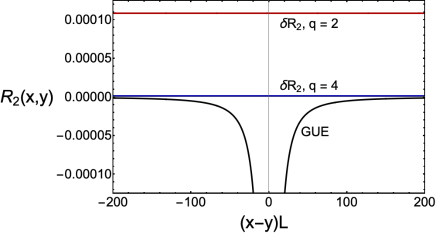
Figure 2: Perturbative calculation of the two-point correlator. The GUE result is the $\mu=0$ term in (73), while the correction $\delta R_{2}$ for $q=2$ (red) and $q=4$ (blue) is due to the $\mu\neq 0$ terms. The ratio of the $q=2$ and $q=4$ correction scales as $N^{2}$, and in the figure its value is 142.

The only way out seems to be that interaction terms between the zero modes ($|\mu|=0$ or $|\mu|=N$ terms) and the massive modes ($|\mu|\neq 0,N$ terms) are important for $q=2$ while their contributions cancel for $q=4$. The details of this cancellation are not clear, in particular because the lowest order contribution of such terms was large in the complex SYK model Verbaarschot1984 . Since $T_{\mu}\sim 1-2|\mu|q/N+\cdots$, the $|\mu|\neq 0$ terms are strongly suppressed with respect to the $|\mu|=0$ or $|\mu|=N$ terms for $x\to y$. For $\mu$ values with ${N\choose|\mu|}\gg 1$ we have that $T_{\mu}\ll 1$. Therefore, we can approximate the correction to the GUE result by expanding the denominator to first order in $T_{\mu}$. In the center of the spectrum this gives the result

$$-\frac{1}{2D^{2}}\sum_{|\mu|}{N\choose|\mu|}T_{\mu}^{2}=-2{N\choose q}^{-1},$$ (77)

so that the correction to the two point correlator is given by

$$\delta R_{2}=\frac{1}{2\pi^{2}}{N\choose q}^{-1}.$$ (78)

In terms of the unfolded energy difference $\omega=(x-y)\rho(0)$, we find

$$\frac{\bar{\rho}_{2c}(\omega)}{\bar{\rho}^{2}(0)}=\rho_{2}^{\rm GUE}(\omega)+\frac{1}{2}{N\choose q}^{-1},$$ (79)

which is in agreement with the results in figure 2. Note that we only get the universal GUE result if we rescale by the saddle point result for the spectral density which differs by $O(1)$ from the correct SYK result.

This result agrees with Altland-ml-2017eao , where it was argued that the corrections to the two-point spectral correlation function are of the form

$$\rho_{2}(\omega)=\rho_{2}^{\rm GUE}(\omega)+\frac{\Delta^{2}}{2\pi^{2}}{\rm Re}\sum_{k=1}^{N/4}{N\choose 2k}\frac{1}{(i\omega+\epsilon(2k))^{2}},$$ (80)

where ${N\choose 2k}$ is the degeneracy of massive modes with mass $\epsilon(k)$, and $\Delta=\pi\sigma/D$ is the level spacing in the center of the band. The $\epsilon(k)$ are given by

$$\epsilon(k)=\sigma(T_{k}^{-1}-1).$$ (81)

Since $T_{k}\sim 1/N^{q}$, the $\epsilon(k)$ are much larger than the span of the spectrum, while $\omega\ll N$. The correlator of Altland-ml-2017eao is thus well-approximated by

$$\rho_{2}(\omega)=\rho_{2}^{\rm GUE}(\omega)+\frac{1}{2}{N\choose q}^{-1},$$ (82)

which is exactly the result from the above perturbative calculation.

Although the $\sigma$-model was derived for arbitrary $N$ and even $q$, it cannot be naively applied to cases with Dyson index $\beta=1$ or $\beta=4$. As was discussed at end of appendix A, the reason is that the $|\mu|=0$ term after the Fierz transformation, gives the GUE result. To extract the GOE result, we have exploited the symmetry of the $\gamma$ matrices for $N\pmod{8}=0$ before the Fierz transformation. Then the $|\mu|=0$ terms include the Cooperon contributions characteristic of the GOE result. Similar arguments can be made for the $\beta=4$ case.

5.2.1 Higher order corrections

It becomes increasingly hard to calculate higher order corrections to the loop-expansion of the two-point correlation function. Such terms are important for ensemble fluctuations that go beyond scale fluctuations. We only calculate the three-loop diagram given by

$$\mathchoice{\vbox{\hbox to0.0pt{\kern 21.21461pt\kern 3.1985pt\hbox{\vrule width=0.50003pt,height=0.0pt,depth=4.30554pt\vrule width=46.8141pt,height=0.0pt,depth=0.50003pt\vrule width=0.50003pt,height=0.0pt,depth=4.30554pt}\hss}\vskip 2.15277pt\vskip 4.30554pt}}{\vbox{\hbox to0.0pt{\kern 21.21461pt\kern 3.1985pt\hbox{\vrule width=0.50003pt,height=0.0pt,depth=4.30554pt\vrule width=46.8141pt,height=0.0pt,depth=0.50003pt\vrule width=0.50003pt,height=0.0pt,depth=4.30554pt}\hss}\vskip 2.15277pt\vskip 4.30554pt}}{\vbox{\hbox to0.0pt{\kern 14.93022pt\kern 2.23895pt\hbox{\vrule width=0.50003pt,height=0.0pt,depth=4.30554pt\vrule width=34.34981pt,height=0.0pt,depth=0.50003pt\vrule width=0.50003pt,height=0.0pt,depth=4.30554pt}\hss}\vskip 2.15277pt\vskip 3.01389pt}}{\vbox{\hbox to0.0pt{\kern 11.80728pt\kern 1.59924pt\hbox{\vrule width=0.50003pt,height=0.0pt,depth=4.30554pt\vrule width=27.10693pt,height=0.0pt,depth=0.50003pt\vrule width=0.50003pt,height=0.0pt,depth=4.30554pt}\hss}\vskip 2.15277pt\vskip 2.15277pt}}\mathchoice{\vbox{\hbox to0.0pt{\kern 50.49287pt\kern 3.1985pt\hbox{\vrule width=0.50003pt,height=0.0pt,depth=8.61108pt\vrule width=30.32988pt,height=0.0pt,depth=0.50003pt\vrule width=0.50003pt,height=0.0pt,depth=8.61108pt}\hss}\vskip 2.15277pt\vskip 4.30554pt}}{\vbox{\hbox to0.0pt{\kern 50.49287pt\kern 3.1985pt\hbox{\vrule width=0.50003pt,height=0.0pt,depth=8.61108pt\vrule width=30.32988pt,height=0.0pt,depth=0.50003pt\vrule width=0.50003pt,height=0.0pt,depth=8.61108pt}\hss}\vskip 2.15277pt\vskip 4.30554pt}}{\vbox{\hbox to0.0pt{\kern 36.00497pt\kern 2.23895pt\hbox{\vrule width=0.50003pt,height=0.0pt,depth=8.61108pt\vrule width=22.23087pt,height=0.0pt,depth=0.50003pt\vrule width=0.50003pt,height=0.0pt,depth=8.61108pt}\hss}\vskip 2.15277pt\vskip 3.01389pt}}{\vbox{\hbox to0.0pt{\kern 28.47969pt\kern 1.59924pt\hbox{\vrule width=0.50003pt,height=0.0pt,depth=8.61108pt\vrule width=16.83153pt,height=0.0pt,depth=0.50003pt\vrule width=0.50003pt,height=0.0pt,depth=8.61108pt}\hss}\vskip 2.15277pt\vskip 2.15277pt}}\mathchoice{\vbox{\hbox to0.0pt{\kern 76.09236pt\kern 3.1985pt\hbox{\vrule width=0.50003pt,height=0.0pt,depth=12.91663pt\vrule width=25.58807pt,height=0.0pt,depth=0.50003pt\vrule width=0.50003pt,height=0.0pt,depth=12.91663pt}\hss}\vskip 2.15277pt\vskip 4.30554pt}}{\vbox{\hbox to0.0pt{\kern 76.09236pt\kern 3.1985pt\hbox{\vrule width=0.50003pt,height=0.0pt,depth=12.91663pt\vrule width=25.58807pt,height=0.0pt,depth=0.50003pt\vrule width=0.50003pt,height=0.0pt,depth=12.91663pt}\hss}\vskip 2.15277pt\vskip 4.30554pt}}{\vbox{\hbox to0.0pt{\kern 55.42456pt\kern 2.23895pt\hbox{\vrule width=0.50003pt,height=0.0pt,depth=12.91663pt\vrule width=17.91162pt,height=0.0pt,depth=0.50003pt\vrule width=0.50003pt,height=0.0pt,depth=12.91663pt}\hss}\vskip 2.15277pt\vskip 3.01389pt}}{\vbox{\hbox to0.0pt{\kern 43.77934pt\kern 1.59924pt\hbox{\vrule width=0.50003pt,height=0.0pt,depth=12.91663pt\vrule width=12.794pt,height=0.0pt,depth=0.50003pt\vrule width=0.50003pt,height=0.0pt,depth=12.91663pt}\hss}\vskip 2.15277pt\vskip 2.15277pt}}\mathchoice{\vbox{\hbox to0.0pt{\kern 88.8864pt\kern 3.1985pt\hbox{\vrule width=0.50003pt,height=0.0pt,depth=17.22217pt\vrule width=19.19106pt,height=0.0pt,depth=0.50003pt\vrule width=0.50003pt,height=0.0pt,depth=17.22217pt}\hss}\vskip 2.15277pt\vskip 4.30554pt}}{\vbox{\hbox to0.0pt{\kern 88.8864pt\kern 3.1985pt\hbox{\vrule width=0.50003pt,height=0.0pt,depth=17.22217pt\vrule width=19.19106pt,height=0.0pt,depth=0.50003pt\vrule width=0.50003pt,height=0.0pt,depth=17.22217pt}\hss}\vskip 2.15277pt\vskip 4.30554pt}}{\vbox{\hbox to0.0pt{\kern 64.38037pt\kern 2.23895pt\hbox{\vrule width=0.50003pt,height=0.0pt,depth=17.22217pt\vrule width=13.43372pt,height=0.0pt,depth=0.50003pt\vrule width=0.50003pt,height=0.0pt,depth=17.22217pt}\hss}\vskip 2.15277pt\vskip 3.01389pt}}{\vbox{\hbox to0.0pt{\kern 50.17635pt\kern 1.59924pt\hbox{\vrule width=0.50003pt,height=0.0pt,depth=17.22217pt\vrule width=9.5955pt,height=0.0pt,depth=0.50003pt\vrule width=0.50003pt,height=0.0pt,depth=17.22217pt}\hss}\vskip 2.15277pt\vskip 2.15277pt}}\mathchoice{\vbox{\hbox to0.0pt{\kern 95.28342pt\kern 3.1985pt\hbox{\vrule width=0.50003pt,height=0.0pt,depth=21.52771pt\vrule width=19.19106pt,height=0.0pt,depth=0.50003pt\vrule width=0.50003pt,height=0.0pt,depth=21.52771pt}\hss}\vskip 2.15277pt\vskip 4.30554pt}}{\vbox{\hbox to0.0pt{\kern 95.28342pt\kern 3.1985pt\hbox{\vrule width=0.50003pt,height=0.0pt,depth=21.52771pt\vrule width=19.19106pt,height=0.0pt,depth=0.50003pt\vrule width=0.50003pt,height=0.0pt,depth=21.52771pt}\hss}\vskip 2.15277pt\vskip 4.30554pt}}{\vbox{\hbox to0.0pt{\kern 68.85828pt\kern 2.23895pt\hbox{\vrule width=0.50003pt,height=0.0pt,depth=21.52771pt\vrule width=13.43372pt,height=0.0pt,depth=0.50003pt\vrule width=0.50003pt,height=0.0pt,depth=21.52771pt}\hss}\vskip 2.15277pt\vskip 3.01389pt}}{\vbox{\hbox to0.0pt{\kern 53.37485pt\kern 1.59924pt\hbox{\vrule width=0.50003pt,height=0.0pt,depth=21.52771pt\vrule width=9.5955pt,height=0.0pt,depth=0.50003pt\vrule width=0.50003pt,height=0.0pt,depth=21.52771pt}\hss}\vskip 2.15277pt\vskip 2.15277pt}}{\rm tr}P_{11}\alpha\,{\rm tr}P_{22}\alpha\,{\rm tr}\,\alpha\alpha\alpha\alpha\alpha\alpha\alpha\alpha.$$ (83)

We find

$$\frac{1}{n}\frac{1}{D}\left\langle\frac{\sqrt{D}}{\sigma}{\rm tr}P_{11}\alpha_{0}\frac{1}{n}\frac{1}{D}\frac{\sqrt{D}}{\sigma}{\rm tr}P_{22}\alpha_{0}\frac{1}{8}\textrm{Tr}\left(\frac{-\bar{G}\sigma}{\sqrt{D}}\sum_{\mu}{}^{{}^{\prime}}\alpha_{\mu}X^{U}_{\mu}\right)^{8}\right\rangle$$ (84)

$$=3\frac{1}{n^{2}D^{5}}\sigma^{6}\bar{G}^{4}(x)\bar{G}^{4}(y)\scalebox{0.97}{\mbox{$\displaystyle\left\langle\!\!{\rm tr}\,\alpha^{11}_{0}{\rm tr}\,\alpha^{22}_{0}\sum_{\mu}{}^{{}^{\prime}}\textrm{Tr}a^{11}_{0}\alpha_{\mu}^{12}X^{U}_{\mu}\alpha_{0}^{22}\alpha_{\nu}^{21}X^{U}_{\nu}\alpha_{\rho}^{12}X^{U}_{\rho}\alpha_{\mu}^{12}X^{U}_{\mu}\alpha_{\nu}^{21}X^{U}_{\nu}\alpha_{\rho}^{12}X^{U}_{\rho}\!\!\right\rangle$}}$$

$$=3\frac{\sigma^{6}}{D^{5}}\frac{\bar{G}^{4}(x)\bar{G}^{4}(y)}{(1-\bar{G}^{2}(x))(1-\bar{G}^{2}(y))}$$

$$\quad\times\sum_{\mu\nu\rho}{}^{{}^{\prime}}\frac{T_{\mu}}{1-T_{\mu}\sigma^{2}G(x)G(y)}\frac{T_{\nu}}{1-T_{\nu}\sigma^{2}G(x)G(y)}\frac{T_{\rho}}{1-T_{\rho}\sigma^{2}G(x)G(y)}\textrm{Tr}X^{U}_{\mu}X^{U}_{\nu}X^{U}_{\rho}X^{U}_{\mu}X^{U}_{\nu}X^{U}_{\rho}.$$

There is another remarkable combinatorial identity (note that there is no prime)

$$\frac{1}{D^{4}}\sum_{\mu\nu\rho}T_{\mu}T_{\nu}T_{\rho}\textrm{Tr}X^{U}_{\mu}X^{U}_{\nu}X^{U}_{\rho}X^{U}_{\mu}X^{U}_{\nu}X^{U}_{\rho}=16(-1)^{q/2}{N\choose q}^{-3}\frac{N!}{(N-3q/2)!((q/2)!)^{3}},$$ (85)

which can be proved by applying the Fierz transformation (161) to $\sum_{\mu}T_{\mu}X^{U}_{\mu}X^{U}_{\nu}$ and the same for the sum over $\nu$ and $\rho$. The sum is only nonzero when the summation indices are either all even or all odd. Since the sum over the many-body space is only over the even indices up to $N/2$, we thus get an overall combinatorial factor of 1/16, so that the total contribution of the diagram (83) to the 33 moment is given by

$$3(-1)^{q/2}{N\choose q}^{-3}\frac{N!}{(N-3q/2)!((q/2)!)^{3}},$$ (86)

which together with the last term of equation (73) gives the correct result for the 33 moment after using the identity

$$\frac{1}{D^{2}}\frac{1}{4}\sum_{|\mu|=0}^{N}{N\choose|\mu|}T_{\mu}^{3}={N\choose q}^{-3}\frac{N!}{(N-3q/2)!((q/2)!)^{3}}.$$ (87)

This agrees with the moment calculation in section 6, and is a very nontrivial check of the correctness of the $\sigma$-model calculation.

5.3 Does the expansion in powers of the resolvent of the semicircle make
sense?

The $\sigma$-model results in an expansion of the resolvent of the SYK model in powers of $g_{0}(z)=z/2-\sqrt{z^{2}-4}/2$:

$$G(z)=\sum_{k}a_{k}g_{0}^{2k+1}(z).$$ (88)

Each of the terms has a cut in the complex plane on the interval $[-2,2]$, while the resolvent of the SYK model has a cut beyond that. In the Q-Hermite approximation, the cut is located on the interval

$$\left[-\frac{2}{1-\eta},\frac{2}{1-\eta}\right],$$ (89)

where $\eta$ is given in equation (7). Since the resolvent of the Q-Hermite spectral density is known analytically, we can get the coefficients $a_{k}$ in this case,

$$a_{k}=\sum_{p=0}^{k}(-1)^{k+p}{k+p\choose k-p}\tilde{M}^{\text{QH}}_{2p}(\eta)$$ (90)

with

$$\tilde{M}^{\text{QH}}_{2p}(\eta)=\frac{1}{(1-\eta)^{p}}\sum_{k=-p}^{p}(-1)^{k}\eta^{k(k-1)/2}{2p\choose p+k}.$$ (91)

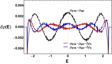
Figure 3: The difference of the spectral density of the SYK model, $\rho_{\rm SYK}(E)$, and three different approximations. First, the Q-Hermite approximation, $\rho_{\rm QH}(E)$ (black curve). Second and third, the expansion in powers of the resolvent of the semicircle scaled to the support of the Q-Hermite result to 7th order, $\rho_{\rm QH}(E)+\delta\rho_{3}$ (blue curve), and 9th order, $\rho_{\rm QH}(E)+\delta\rho_{4}$ (red curve).

The spectral density that can be derived from derived from (90) is strongly oscillating, and to make sense of the result, the asymptotic series has to be resummed. Based on the case $\eta=1$, one might think that a Borel resummation might lead to a convergent result Verbaarschot1984 , but we were not able to work out the sums for arbitrary $\eta$. However, we can also expand the resolvent in powers of

$$g_{0\eta}(z)=\sqrt{1-\eta}\left({\frac{z}{2}\sqrt{1-\eta}}-\frac{1}{2}\sqrt{z^{2}(1-\eta)-4}\right).$$ (92)

Naively, because the spectrum corresponding to this resolvent has the same support as the weight function of the Q-Hermite polynomials, we expect that this gives a much better expansion. It turns out that the expansion is surprisingly simple Cappelli-1998 ; Berkooz-ml-2018jqr

$$G_{\rm QH}(z)=\sum_{k=0}^{\infty}\frac{\eta^{k(k+1)/2}}{(\eta-1)^{k}}g_{0\eta}^{2k+1}(z).$$ (93)

Since $|g_{0\eta}|=\sqrt{1-\eta}$ and $|\eta|<1$, this expansion is convergent for the Q-Hermite spectral density.

We could also expand the exact resolvent of the SYK model in powers of $g_{0\eta}^{2k+1}(z)$, by requiring that the moments up to a given order are the same. To the eighth order in the moments this gives

$$G_{\rm SYK}(z) =G^{\rm QH}(z)+(M_{6}^{\rm SYK}-M_{6}^{\rm QH})g_{0\eta}^{7}(z)$$

$$\quad+\left(M_{8}^{\rm SYK}-M_{8}^{\rm QH}+\frac{7(M_{6}^{\rm SYK}-M_{6}^{\rm QH})}{-1+\eta}\right)g_{0\eta}^{9}(z)$$ (94)

with corresponding corrections $\delta\rho_{3}$ ($k=3$) and $\delta\rho_{4}$ ($k=4$) to the spectral density.

For $N=32$ the sixth order result agrees better than $0.1\%$ with the exact result, which is much better than the Q-Hermite approximation, see figure 3. The eighth order correction only gives a slight improvement.

6 Analytical calculation of the fluctuations of the expansion coefficients

In this section, we calculate the covariance matrix of the expansion coefficients of the spectral density in terms of the Q-Hermite density and the Q-Hermite polynomials,

$$\rho(x)=\rho_{QH}(x)\sum_{i=0}c_{i}H_{i}^{\eta}(x).$$ (95)

We will obtain explicit results for the expectation values $\langle c_{k}c_{l}\rangle$ for $k,l\leq 6$. Since the numerics in this paper are done in dimensionless units, and spectral densities are normalized to one, it is convenient to study the rescaled (by the many-body variance $\sigma$), and normalized moments

$$\tilde{M}_{m,n}:=\frac{\langle\textrm{Tr}H^{m}\textrm{Tr}H^{n}\rangle}{2^{N}\sigma^{m+n}},\qquad\tilde{M}_{n}:=\tilde{M}_{0,n},$$ (96)

which were already introduced in section 4.

The covariances of the stochastic coefficients $c_{i}$ are related to the double-trace moments by

$$\begin{split}\tilde{M}_{m,n}&=\sum_{i,j=0}\langle c_{i}c_{j}\rangle\int dxdyx^{m}y^{n}\rho_{QH}(x)\rho_{QH}(y)H_{i}^{\eta}(x)H_{j}^{\eta}(y)\\ &=\sum_{i,j}f_{mi}f_{nj}\langle c_{i}c_{j}\rangle=\sum_{i,j}f_{mi}\langle c_{i}c_{j}\rangle(f^{T})_{jn},\end{split}$$ (97)

where

$$f_{mi}=\int dxx^{m}\rho_{QH}(x)H_{i}^{\eta}(x).$$ (98)

Note that because the $H_{i}^{\eta}(x)$ are orthogonal with respect to $\rho_{QH}(x)$ we have $f_{mi}=0$ for $m<i$, which means $f_{mi}$ forms a triangular matrix of infinite size. The coefficients $c_{mi}$ also vanish when $m+i$ is odd. The covariance matrix $\langle c_{i}c_{j}\rangle$ is given by

$$\langle c_{i}c_{j}\rangle=\sum_{m,n}(f^{-1})_{im}\tilde{M}_{m,n}((f^{T})^{-1})_{nj}.$$ (99)

Since the inverse of the triangular matrix $f_{mi}$ must also be triangular, we can consistently truncate equation (99) up to some finite values of $i,j,m$ and $n$. An efficient way to calculate the $f_{mi}$, using that $H_{i}^{\eta}(x)=\sum_{k}a_{ik}^{\eta}x^{k}$, is

$$f_{mi}=\sum_{k=0}^{i}a_{ik}^{\eta}\tilde{M}_{m+k}^{\text{QH}}(\eta),$$ (100)

where the moments $\tilde{M}_{m+k}^{\text{QH}}(\eta)$ can be obtained from Riordan-Touchard formula, introduced earlier as equation (91):

$$\tilde{M}^{\text{QH}}_{2p}=\frac{1}{(1-\eta)^{p}}\sum_{k=-p}^{p}(-1)^{k}\eta^{k(k-1)/2}{2p\choose p+k}.$$ (101)

An important caveat is in order: in the numerics we used an irreducible block of the random Hamiltonians to calculate the two-point correlations, which is the appropriate thing to do for probing RMT universalities. This means we really should be looking at

$$2^{-N+2}\sigma^{-m-n}\left\langle\textrm{Tr}\left(\frac{1+\gamma_{c}}{2}H^{m}\right)\textrm{Tr}\left(\frac{1+\gamma_{c}}{2}H^{n}\right)\right\rangle$$ (102)

instead of $\tilde{M}_{m,n}$, where $\gamma_{c}$ is the chirality Dirac matrix in even dimensions. However, since $\gamma_{c}$ is a product of $N$ different Dirac matrices, we have $\textrm{Tr}\left(\gamma_{c}H^{m}\right)=0$ realization by realization if $m<N/q$. For $N=32$ and $q=4$, this means equation (102) coincide with $\tilde{M}_{m,n}$ for the double-trace moments up to $m=7$ and $n=7$, which means we might as well use $\tilde{M}_{m,n}$ for the calculation of $\langle c_{i}c_{j}\rangle$ up to $i=7$ and $j=7$. In this paper we will not go beyond $\tilde{M}_{6,6}$ due to computational complexity, but we do caution that $\textrm{Tr}\left(\gamma_{c}H^{m}\right)$ must be confronted for higher moments.

6.1 General expression for double-trace Wick contractions

In this section we give a general expression for double-trace contractions contributing to rescaled double-trace moments $\tilde{M}_{m,n}$.

Figure 4: Three contractions in $\tilde{M}_{4,4}$: ($a$) is part of the disconnected piece in $\tilde{M}_{4,4}$; ($b$) has four cross links; ($c$) has two cross links and two single-trace links.

Since the ensemble average is taken over a Gaussian distribution and thus reduced to a sum over Wick contractions, we can represent the double traces as chord diagrams. Since there are two traces, we will use two different horizontal lines to attach the chords on. Such horizontal lines are called backbones in some of the chord diagram literature. For example, in figure 4 we draw three chord diagrams with two backbones that represent some of the contractions that contribute to $\tilde{M}_{4,4}$. In a self-evident manner they represent (we will not adopt Einstein’s summation convention unless otherwise stated)

$$\begin{split}&(a)\quad 2^{-N}\binom{N}{q}^{-4}\sum_{\alpha_{1},\alpha_{2},\beta_{1},\beta_{2}}\textrm{Tr}(\Gamma_{\alpha_{1}}\Gamma_{\alpha_{2}}\Gamma_{\alpha_{2}}\Gamma_{\alpha_{1}})\textrm{Tr}(\Gamma_{\beta_{1}}\Gamma_{\beta_{2}}\Gamma_{\beta_{1}}\Gamma_{\beta_{2}})\\ &(b)\quad 2^{-N}\binom{N}{q}^{-4}\sum_{a_{1},a_{2},a_{3},a_{4}}\textrm{Tr}(\Gamma_{a_{1}}\Gamma_{a_{2}}\Gamma_{a_{3}}\Gamma_{a_{4}})\textrm{Tr}(\Gamma_{a_{1}}\Gamma_{a_{4}}\Gamma_{a_{3}}\Gamma_{a_{2}})\\ &(c)\quad 2^{-N}\binom{N}{q}^{-4}\sum_{a_{1},a_{2},\beta_{1},\beta_{2}}\textrm{Tr}(\Gamma_{a_{1}}\Gamma_{\beta_{1}}\Gamma_{a_{2}}\Gamma_{\beta_{1}})\textrm{Tr}(\Gamma_{a_{2}}\Gamma_{a_{1}}\Gamma_{\beta_{2}}\Gamma_{\beta_{2}})\end{split}$$

Note ($a$) belongs to the disconnected part of $\tilde{M}_{4,4}$, since all the chords connect only within single traces, and we call such chords single-trace links; on the other hand ($b$) and ($c$) belong to the connected part of $\tilde{M}_{4,4}$ because both contain chords that go from one backbone to the other, and we call such chords cross links. It is important to keep in mind that notationally we used

• Latin-letter subscripts on the cross-linked $\Gamma$’s and

• Greek-letter subscripts on the single-trace-linked $\Gamma$’s.

The combinatorics for double-trace moments are much like the single-trace moments discussed in Garcia-Garcia-ml-2018kvh , with two additional rules for the $d$ variables which are the cardinality of the regions in the Venn diagram of overlapping indices. In other words, $d_{a_{i_{1}}a_{i_{2}}\ldots a_{i_{k}}}$ is the number of elements common and only common to the sets $a_{i_{1}},a_{i_{2}},\ldots,a_{i_{k}}$ (naturally, $i_{1},\ldots,i_{k}$ are all different from each other in this definition). The additional rules are as follows:

• The $d$-variables with odd number of Latin-letter subscripts (and an arbitrary number of Greek-letter subscripts) must be set to zero.

• Kronecker deltas are needed to enforce that the total number of indices corresponding to one vertex is $q$.

More explicitly, a double-trace chord diagram $G$ has a value of

$$\begin{split}(-1)^{qE_{G}}\binom{N}{q}^{-V_{G}}\sum_{\{d\}}^{q}&(-1)^{c(G)}\mathcal{M}(\{d\})\Delta(\{d\}),\end{split}$$ (103)

where

$$\begin{split}V_{G}&=\text{number of chords in }G,\\ E_{G}&=\text{number of chord intersections in }G,\\ c(G)&=\text{sum of $c$-variables whose subscripts denote intersecting chords,}\\ &\quad\text{ see equation~{}(\ref{c-def}) for a definition},\\ \{d\}&=\text{set of all $d$-variables with even number of Latin-letter subscripts,}\\ \mathcal{M}&=\text{multiplicity factor due to partitioning $N$,}\\ \Delta&=\text{product of Kronecker deltas enforcing the constraints $d_{a_{i}}=0$.}\end{split}$$ (104)

More specifically, if there are $L$ cross links and $V_{G}-L$ single-trace links,

$$\{d\} =\{d_{a_{i_{1}}\ldots a_{i_{r}}\beta_{j_{1}}\ldots\beta_{j_{s}}}|r\text{ is even},\{i_{1},\ldots,i_{r}\}\subset\{1,\ldots,L\},\{j_{1},\ldots,j_{s}\}\subset\{1,\ldots,V_{G}-L\}\},$$

$$\mathcal{M}(\{d\}) =\frac{N!}{(N-qV_{G}+\sum_{k=2}^{V_{G}}(k-1)d_{k})!}\frac{1}{\prod_{\{d\}}d_{\{a\}\{\beta\}}!},$$

$$\Delta(\{d\}) =\prod_{i=1}^{L}\delta\left(q-\sum_{\cdots}d_{a_{i}\ldots}\right),$$ (105)

in which

$$\begin{split}d_{k}&=\text{sum of all $d$-variables with $k$ subscripts,}\\ \prod_{\{d\}}d_{\{a\}\{\beta\}}!&=\text{product of the factorials of all $d$-variables in $\{d\},$}\\ \sum_{\cdots}d_{a_{i}\ldots}&=\text{sum of all $d$-variables containing $a_{i}$ as one of the subscripts.}\end{split}$$ (106)

As one can see, the most general description of the double trace combinatorics is unfortunately convoluted. We encourage the readers to look into the application of (103)–(106) to the examples of $\tilde{M}_{3,3}$ and $\tilde{M}_{3,5}$ illustrated in appendix D.

6.2 Some useful properties of double-trace moments

There are a few other properties of double-trace contractions that will be useful for evaluating double-trace averages:

1. $\tilde{M}_{m,n}=0$ if $m+n$ is odd. Hence we only need to concern ourselves with the cases of $m+n$ being even.

2. $\textrm{Tr}H=0$ even before taking average, so $\tilde{M}_{1,n}=0$ for all $n$.

3. $\textrm{Tr}(\Gamma_{\alpha}\Gamma_{\beta})=\delta_{\alpha\beta}$, this implies $\tilde{M}_{2,2n}-\tilde{M}_{2}\tilde{M}_{2n}=\binom{N}{q}^{-1}2n\tilde{M}_{2n}$, or more generally

   $$\tilde{M}_{m,n}^{(2)}=\binom{N}{q}^{-1}2mn\tilde{M}_{2m}\tilde{M}_{2n},$$ (107)

   where $\tilde{M}_{m,n}^{(2)}$ denotes the sum over all contractions that contribute to $\tilde{M}_{m,n}$ with exactly two cross links. This gives a precise meaning to equation (30).

4. For any $N$, there exists a charge conjugation matrix, either $C_{+}$ or $C_{-}$ (or both), such that $C^{-1}_{\pm}\gamma_{i}C_{\pm}=\pm\gamma_{i}^{T}$, this implies the following reflection identity

   $$\textrm{Tr}\left(\Gamma_{\alpha_{1}}\Gamma_{\alpha_{2}}\ldots\Gamma_{\alpha_{k}}\right)=(-1)^{kq(q-1)/2}\textrm{Tr}\left(\Gamma_{\alpha_{k}}\Gamma_{\alpha_{k-1}}\ldots\Gamma_{\alpha_{1}}\right),$$ (108)

   where we also used

   $$\gamma_{i_{q}}\gamma_{i_{q-1}}\cdots\gamma_{i_{2}}\gamma_{i_{1}}=(-1)^{q(q-1)/2}\gamma_{i_{1}}\gamma_{i_{2}}\cdots\gamma_{i_{q-1}}\gamma_{i_{q}}.$$ (109)

   This reflection, together with the cyclic permutations of the $\Gamma$’s, gives rise to a natural dihedral group action on the traces.

5. If all but one subscript in the traces are summed, the result is a constant independent of the remaining unsummed subscript, see appendix D of reference Garcia-Garcia-ml-2018kvh . This implies every contraction’s value must contain a factor of $\binom{N}{q}$. This means each term contributing to $2^{-N}\langle\textrm{Tr}H^{m}\textrm{Tr}H^{n}\rangle$ will factorize into $\binom{N}{q}$ times another integer (and times $\sigma^{m+n}$). Analogous to the single trace situation, this implies a further factorization property of a special class of double-trace contractions: if a single-trace link intersects with exactly one cross link and nothing else, then this chord diagram factorizes into a double-trace diagram with this single-trace link removed and a single-trace diagram of two chords with one intersection (whose value is $\eta$ of (7)). Figure 5 illustrates such an example.

   Figure 5: The factorization of a chord diagram.

6.3 Low-order covariances of Q-Hermite expansion coefficients

In this section we give explicit results for the covariances up to sixth order for $N=32$ and $q=4$ which is the case we study numerically later. Apart from the moments $\tilde{M}_{2,2m}$ given by equation (107), we also need the following results:

$$\tilde{M}_{3,3} =\frac{1701}{161640200} \qquad\tilde{M}_{3,5} =\frac{4835943}{72657269900}$$

$$\tilde{M}_{4,4} =\frac{14912736088383}{2906290796000} \qquad\tilde{M}_{4,6} =\frac{201028717157105439}{13063777128020000}$$

$$\tilde{M}_{5,5} =\frac{8812289619}{20902043404832} \qquad\tilde{M}_{6,6} =\frac{2710088957667107403387}{58721678190449900000}.$$

Then using equation (99) up to $i,j,m,n=6$, we obtain for $N=32,q=4$ the following nonzero covariances up to $i,j\leq 6$:

$$\langle c_{0}^{2}\rangle =1, \quad\langle c_{0}c_{6}\rangle =-6.4397\times 10^{-3}, \langle c_{0}c_{2}\rangle =0,\quad\langle c_{0}c_{7}\rangle=0,$$

$$\langle c_{2}^{2}\rangle =3.47581\times 10^{-5}, \quad\langle c_{2}c_{4}\rangle =1.78799\times 10^{-5}, \quad\langle c_{2}c_{6}\rangle =1.11629\times 10^{-5},$$

$$\langle c_{3}^{2}\rangle =3.68918\times 10^{-6}, \quad\langle c_{3}c_{5}\rangle =2.74962\times 10^{-6},$$

$$\langle c_{4}^{2}\rangle =9.59628\times 10^{-6}, \quad\langle c_{4}c_{6}\rangle =6.154203\times 10^{-6},$$

$$\langle c_{5}^{2}\rangle =2.11476\times 10^{-6}, \quad\langle c_{6}^{2}\rangle =4.55032\times 10^{-5}.$$

Note that $c_{0}=1$ and $c_{1}=0$ even before averaging. These numbers agree reasonably well with the numerical results presented in figure 10. General expressions for low-order moments are given in appendix E.

7 Numerical analysis of spectral correlations

In this section we analyze the spectral correlations of the eigenvalues obtained by diagonalization of the SYK Hamiltonian for $N=32$. In section 7.1 we discuss the number variance. The fluctuations due to ensemble averaging are analyzed in section 7.2 and spectral form factor is evaluated in 7.3.

7.1 Number variance

If $\langle\rho(x)\rangle$ is the average spectral density, then the average number of levels in an interval of width $\Delta$ is given by

$$\bar{n}=\int_{x-\Delta/2}^{x+\Delta/2}\langle\rho(y)\rangle dy.$$ (110)

The actual number of levels in the interval is equal to

$$n=\int_{x-\Delta/2}^{x+\Delta/2}\rho(y)dy,$$ (111)

so that the deviation from the average number is given by

$$\delta n=\int_{x-\Delta/2}^{x+\Delta/2}(\rho(y)-\langle\rho(y)\rangle)dy.$$ (112)

The variance of $\delta n$ as a function of $\bar{n}$ is known as the number variance,

$$\Sigma^{2}(\bar{n})\equiv{\rm var}\{\delta n\}.$$ (113)

The average eigenvalue density can be obtained in two ways. First as the ensemble average of the spectral density for a very large ensemble. Second, for large matrices, as a fit of a smooth function, $\rho_{\text{smo}}(x)$, to the spectral density of a single disorder realization. If the two are the same for $N\to\infty$, we speak of spectral ergodicity Pandey-1979 . Even if $\rho_{\text{smo}}(x)-\langle\rho(x)\rangle\sim 1/N$, it can give a large contribution to the number variance for intervals where $n$ is no longer much smaller than $N$. In particular, this may happen in many-body systems where the number of levels increases exponentially with the number of particles.

To calculate the number variance as a function of the average number of levels in an interval we need to know $x$ as a function of the number of levels with energy less than $x$. In other words, we have to invert the mode number function defined as

$$N(x)=\int_{-\infty}^{x}\langle\rho(y)\rangle dy.$$ (114)

Since the number of eigenvalues in an interval does not change under a coordinate transformation, it is simplest to invert (114) in coordinates where the level density is constant. If the constant is equal to one, the transformation is particularly simple:

$$dx^{\prime}=\langle\rho(x)\rangle dx.$$ (115)

The spacing of the levels in the new coordinates is thus given by

$$x_{k+1}^{\prime}-x_{k}^{\prime}=\langle\rho(x_{k})\rangle(x_{k+1}-x_{k}),$$ (116)

and the new level sequence is obtained by adding the differences,

$$x_{k}^{\prime}=\sum_{p=1}^{k-1}\langle\rho(x_{p-1})\rangle(x_{p}-x_{p-1})\approx\int_{-\infty}^{x_{k}}dy\langle\rho(y)\rangle.$$ (117)

This procedure is usually referred to as unfolding. We emphasize that this procedure is not necessary for the calculation of the number variance, but it makes it much more convenient to invert the mode number function $N(x)$.

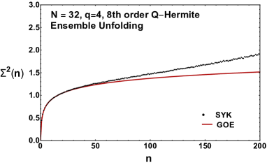
Figure 6: The number variance of the eigenvalues of an ensemble of 400 SYK Hamiltonians versus the length of the interval $n$. In the left figure we also show a quadratic fit (red curve) and the grey band depicts the error bars. The right figure which is a blow-up of the left figure also shows the number variance of the GOE (red curve).

As was argued in section 4, due to the relative error in the spectral density of ${N\choose q}^{-1/2}$, for large $\bar{n}$ the number variance behaves as

$$\Sigma^{2}(\bar{n})\sim\frac{1}{2}{N\choose q}^{-1}\bar{n}^{2},$$ (118)

which agrees with results obtained previously Altland-ml-2017eao ; Garcia-Garcia-ml-2018ruf for $q=4$ and $q=3$. The Thouless energy scale can thus be estimated as

$$n_{\rm Th}\sim{N\choose q}^{1/2}.$$ (119)

To calculate the number variance, we unfold the spectrum by means of a fit to the ensemble average of the spectral density including up to eighth order Q-Hermitian polynomials. The results are shown in figure 6 where we plot $\Sigma^{2}(\bar{n})$ (black points) versus the average number of levels $\bar{n}$ in an interval for an ensemble of 400 SYK Hamiltonians with $N=32$. For small $\bar{n}<40$ we see excellent agreement with the GOE (red curve) (see right figure), but for large distances, the number variance grows quadratically, $\Sigma^{2}(\bar{n})\sim(\bar{n}/293)^{2}$. The latter result is in good agreement with analytical result of $\bar{n}^{2}/2{N\choose q}$ (which gives $(\bar{n}/268)^{2}$ for $N=32$ and $q=4$).

7.2 The effect of ensemble averaging

As mentioned before, the ensemble fluctuations contribute to the number variance as

$$\Sigma^{2}(\bar{n})=\frac{1}{2}{N\choose q}^{-1}\bar{n}^{2}.$$ (120)

This contribution can be subtracted by rescaling the eigenvalues of each realization of the ensemble according to its width French1973 ; Flores_2001 ; Altland-ml-2017eao ; Garcia-Garcia-ml-2018ruf ; Gharibyan-ml-2018jrp . However, this is only the first term in a “multi-pole” expansion, and in this section we systematically study the long-wavelength fluctuations that give rise to the discrepancy between spectral correlations in the SYK model and random matrix theory.

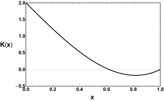
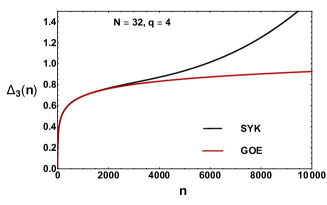
Figure 7: The kernel of the $\Delta_{3}$ statistic (left) projects out the quadratic part of the number variance resulting in agreement with random matrix theory to much larger distances (right figure).

This quadratic contribution (120) due to the scale fluctuations is projected out in the $\Delta_{3}$ statistic defined by

$$\Delta_{3}(\bar{n})=\int_{0}^{1}duK(u)\Sigma^{2}(u\bar{n}),$$ (121)

with smoothening kernel $K(u)$ given by (see figure 7)

$$K(u)=2(1-2u+u^{3}).$$ (122)

Since $\int_{\sqrt{2}-1}^{1}K(u)du=0$, in case where the number variance depends only weakly on $\bar{n}$, the $\Delta_{3}(\bar{n})$ statistic in essence only measures level fluctuations up to $(\sqrt{2}-1)\bar{n}$ and roughly corresponds to the number variance at $\bar{n}/4$. Indeed, as is shown in figure 7, the $\Delta_{3}$ statistic agrees with the GOE to much larger values of $\bar{n}$ with a Thouless energy that is about 2000 level spacings.

Next we explore the origin of other contributions to the discrepancy between the SYK model and the Wigner-Dyson ensembles. We do this by eliminating the “collective” fluctuations of the eigenvalues of each realization of the ensemble in which a macroscopic number of eigenvalues moves together relative to the ensemble average. This is achieved by calculating the average mode number by fitting a smooth function to the spectral density of a single configuration. The smoothened spectral density can be obtained in a systematic way by expanding it in Q-Hermite polynomials, truncated at $l$-th order:

$$\bar{\rho}_{QH,l}(x)=\rho_{QH}(x)\left[1+\sum_{k=1}^{l}c_{k}H^{\eta}_{k}(x)\right].$$ (123)

The coefficients $c_{k}$ can be calculated by minimizing the $L_{2}$ norm excluding a small fraction of the eigenvalues in both tails of the spectrum. Generically, all even and odd coefficients are nonvanishing with an ensemble average that agrees with the fit to the average spectral density obtained in equation (12).

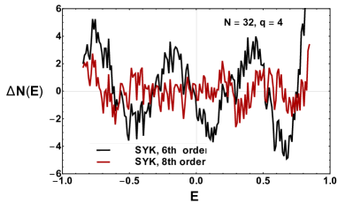
Figure 8: The difference between the mode number function of the SYK model and the Q-Hermite approximation to order 2 (left, black), 4 (left, red), 6 (right, black) and 8 (right, red). At order 8, the systematic fluctuations are of the same order as the statistical fluctuations.

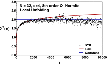
Figure 9: Number variance (black points) versus the average number of levels $n$ in the interval. The average number of eigenvalues in the interval is calculated from an eighth order Q-Hermite fit to the mode number density of each configuration. In the left figure we compare the data to a constant determined by the data for $2500<\bar{n}<4000$. The right figure is a blow-up of the left figure for smaller $\bar{n}$. In both figures, the GOE result is depicted by the red curve.

In figure 8 we show the difference of the cumulative spectral density of the SYK model and $\bar{\rho}_{\rm QH,2}$, $\bar{\rho}_{\rm QH,4}$, $\bar{\rho}_{\rm QH,6}$ and $\bar{\rho}_{\rm QH,8}$. It is clear that for $l=8$ the systematic dependence is of the same order as the statistical fluctuations, and no further gains can be made by including higher values of $l$.

We now calculate the number variance using $\bar{\rho}_{QH,l}$ to determine the number of eigenvalues in the interval for each configuration. We use both ensemble and spectral averaging to reduce the statistical fluctuations. For the latter we choose half-overlapping intervals. In figure 9 we show results for $l=8$. The Thouless energy is about 2000 level spacings, but for large $\bar{n}$ the number variance saturates to a constant and decreases beyond $\bar{n}\approx 6000$. This has two reasons. First, by unfolding configuration by configuration, we have eliminated fluctuations with wavelength larger than about $2^{N/2}/16=2048$. Second, because the total number of eigenvalues is fixed, the variance is suppressed when $\bar{n}$ becomes of the same order as $2^{N/2}/2$.

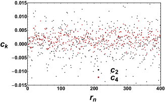
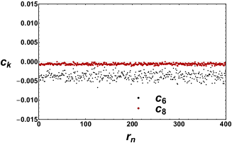
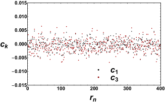
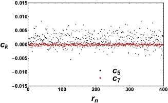
Figure 10: The expansion coefficients $c_{k}$ of the mode number $N(x)$ in the first eight Q-Hermite polynomials versus the realization number $r_{n}$ for an ensemble of 400 realizations.

The coefficients of the expansion of the mode number function $N(x)$ in Q-Hermite polynomials as a function of the ensemble realization number are shown in figure 10. In agreement with our analytical results, the first four coefficients and $c_{5}$ and $c_{7}$ fluctuate about zero, while $c_{6}$ and $c_{8}$ fluctuate about a nonzero value.

Next we study the dependence of the deviation of the number variance from the GOE result on the number of Q-Hermite polynomials that have been taken into account. In figure 11 we show the number variance when an increasing number of coefficients has been fitted to the spectral density of each configuration. In the upper row only $c_{2}$ has been fitted while $c_{3}$ until $c_{8}$ have been put to the their ensemble-averaged values.

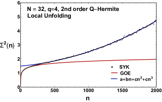
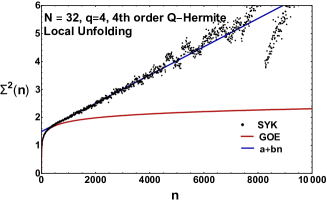
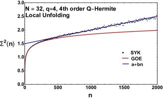
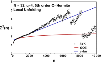
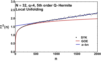
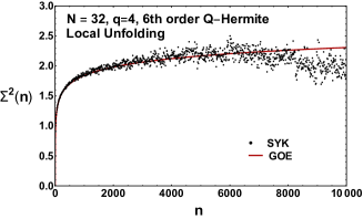
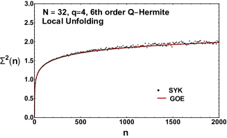
Figure 11: Number variance (black points) versus the average number of levels $n$ in the interval. In the upper row $c_{1}$ and $c_{2}$ are fitted to the mode number for each configuration, in the second row the same for $c_{1},c_{2},c_{3},c_{4}$, and in the third (fourth) row the same for $c_{1},c_{2},c_{3},c_{4},c_{5},(c_{6})$. In the first row the SYK data are fitted to a quadratic $\bar{n}$-dependence, and in the next two rows to a linear one (blue curve). The GOE result is depicted by the red curve. A blow-up of the left figures for smaller $n$ values is shown in the right column.

In the second row, $c_{2}$, $c_{3}$ and $c_{4}$ have been fitted and $c_{5}$, $c_{6}$, $c_{7}$ and $c_{8}$ have been put equal to their ensemble-averaged values. In the third (fourth) row, the first five (six) coefficients have been obtained by fitting while the remaining ones up to order eight have been put equal to their ensemble-averaged values. Because the bulk of the deviation of the spectral density from the Q-Hermite approximation is given by a sixth order polynomial, the number variance is sensitive to whether the length of the interval is commensurate with the distance of the zeros of the polynomial. That is why we observe large jumps (see figure 11 lower left) when the number of intervals used to calculate the number variance changes. When the length of the interval becomes smaller than about half the distance between the zeros of the sixth order Q-Hermite polynomial, this effect is no longer visible. The right column which shows a blow-up of the figures in the left column for small $\bar{n}$ illustrates that the Thouless energy increases gradually with the number of Q-Hermite polynomials that have been taken into account in fitting the local spectral density, until it saturates at a value of $\bar{n}$ corresponding to the shortest wavelength used for unfolding.

For second-order local unfolding, the number variance for large $\bar{n}$ is still quite accurately given by a quadratic $\bar{n}$-dependence, but with a much smaller coefficient than in the case of ensemble averaging, For fourth order and beyond, the quadratic contribution is negligible and the number variance beyond the Thouless energy is very well fitted by a linear $\bar{n}$-dependence.

7.3 Spectral form factor

Alternatively spectral correlations can be studied by means of the connected spectral form factor defined as

$$K_{c}(t)=\int dxdye^{it(x-y)}\rho_{2c}(x,y)=\int dxdye^{it(x-y)}(\langle\rho(x)\rho(y)\rangle-\langle\rho(x)\rangle\langle\rho(y)\rangle).$$ (124)

The second term is the disconnected part. One could also study the spectral form factor without this subtraction Cotler2016 , but in this paper we only consider the connected spectral form factor. Since spectral correlations are universal on the scale of the average level spacing, we have

$$\rho_{2c}(x,y)=\langle\rho(x)\rangle\langle\rho(y)\rangle\rho_{\rm 2,unv}\left((x-y)\langle\rho(x)\rangle\right),$$ (125)

where $\rho_{\rm 2,unv}$ is the universal random matrix result. Therefore, the spectral form factor becomes universal in terms of the variable $t/\langle\rho(x)\rangle$. Its large $N$ limit is thus given by a double scaling limit which receives contributions from all orders in $1/N$ of moments.

We calculate the spectral form factor for the eigenvalues of the Hamiltonian of the SYK model. In order to have a well-behaved sum in equation (124) we need to perform some degree of smoothening which we will do by introducing a Gaussian cutoff of width $w$ with centroid $\bar{E}=0$ Saad-ml-2018bqo ,

$$K_{c}(t)=2\sqrt{\pi}w\int dxdye^{it(x-y)}\frac{e^{-(x-\bar{E})^{2}/2w^{2}}}{\sqrt{2\pi}w}\frac{e^{-(y-\bar{E})^{2}/2w^{2}}}{{\sqrt{2\pi}w}}\rho_{2c}(x,y).$$ (126)

We will evaluate the spectral form factor for the unfolded spectrum with $\langle\rho_{\rm unf}(x)\rangle=1$ and have chosen the prefactor such that for large $t$, when we can use the diagonal approximation, it is equal to unity.

In figures 12 and 14 we show the spectral form factor for the unfolded spectra that were used to calculate the number variance in the previous section. In figure 12, the results for unfolding with the ensemble average are given in the left figure, and for unfolding configuration by configuration with eighth order Q-Hermite polynomials, in the right figure. We used four different values for the width of the Gaussian cutoff. For still larger values of the cutoff, the results are affected significantly by finite size effects. Already for $w=4000$ we observe considerable finite size effects. The GOE result given by

$$K_{\rm GOE}(t/2\pi)=\left.\theta(1-u)\left(2u-u\log(1+2u)\right)+\theta(u-1)\left(2-u\log\frac{2u+1}{2u-1}\right)\right|_{u\to t/2\pi}$$ (127)

is represented by the red curve in both figures. It agrees with the SYK spectra up to very short times. Comparing the two figures, we observe that the spectral fluctuations due to the ensemble average result in a peak at small times. The peak should not be confused with the contribution from the disconnected part of the two-point correlator which is many orders of magnitude larger. For local unfolding there is no peak, and spectral form factor approaches zero for $t\to 0$. Note that without the Gaussian cut-off the spectral form factor $K_{c}(t=0)=0$ because of the normalization of the spectral density. With the cut-off, the spectral form factor at $t=0$ measures the fluctuations of the number of levels inside the Gaussian window. It becomes only zero when the window is larger than the spectral support.

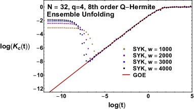
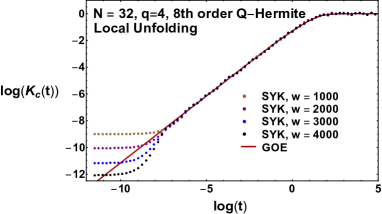
Figure 12: The connected spectral form factor $K_{c}(t)$ versus $t$ using the ensemble averaging for unfolding (left) and unfolding configuration by configuration including Q-Hermite polynomials up to eighth order (right).

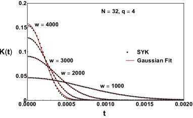
Figure 13: The spectral form factor for small $t$ obtained by using the ensemble average of the spectral density for unfolding (black points). The results are fitted to a Gaussian (red curve).

In figure 13 we show the form factor for small times on a linear scale. Then the constant part of the two-point correlator gives the contribution

$$2\sqrt{\pi}wb_{N}e^{-t^{2}w^{2}}.$$ (128)

For $w\to\infty$ this converges to the $\delta$-function

$$2\pi b_{N}\delta(t).$$ (129)

The constant $b_{N}$ can be approximated by (see equation (27))

$$b_{N}=\frac{1}{2}{N\choose q}^{-1}=1.39\times 10^{-5}.$$ (130)

In figure 13, we fit the parameters $b_{N}$ and $w$ to the SYK data. For $w\leq 3000$, the fitted value of $b_{N}\approx 1.26\times 10^{-5}\approx 1/282^{2}$ is close to the theoretical value given in equation (130), while for $w=4000$ it is 15 % smaller.

The number variance is related to the spectral form factor by a an integral over a smoothening kernel Delon-1991 :

$$\Sigma^{2}(\bar{n})=\frac{\bar{n}^{2}}{2\pi}\int_{-\infty}^{\infty}dtK(t)\left(\frac{\sin(\bar{n}t/2)}{\bar{n}t/2}\right)^{2}.$$ (131)

Therefore, the $\delta(t)$ contribution to the spectral form factor leads to a quadratic dependence of the number variance,

$$\Sigma^{2}(\bar{n})=b_{N}\bar{n}^{2}.$$ (132)

If $K(t)$ remains finite for $t\to 0$ the large $\bar{n}$ limit of the number variance is given by

$$\Sigma^{2}(\bar{n})\approx\bar{n}\lim_{\bar{n}\to\infty}K(1/\bar{n}).$$ (133)

In figure 14 we show the spectral form factor for an increasing number of fitted coefficients while the remaining ones up to eighth order are kept equal to the ensemble average. For a fourth or fifth order fit, the spectral form factor seems to approach a constant for $t\to 0$. From equation (131) it is clear that this will result in a linear dependence of the number variance. The coefficient of the linear term for fifth order unfolding is equal to $3.9\times 10^{-4}$ which is in good agreement with the spectral form factor for $t\to 0$ (which is $5.7\times 10^{-4}$, $7.1\times 10^{-4}$, $5.7\times 10^{-4}$ and $3.0\times 10^{-4}$ for $w=1000$, $w=2000$, $w=3000$ and $w=4000$, respectively.)

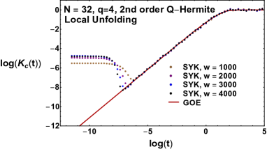
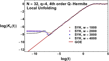
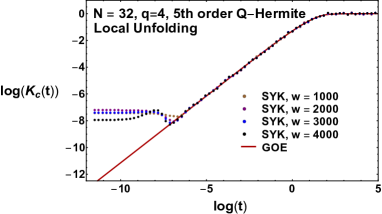
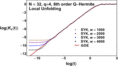
Figure 14: Double logarithmic plot of the spectral form factor for increasing order of the Q-Hermite polynomial used to fit the smoothened spectral density for each configuration.

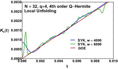
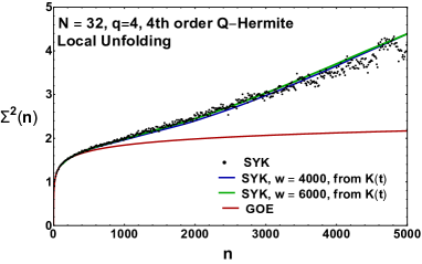
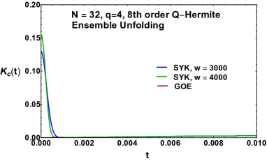
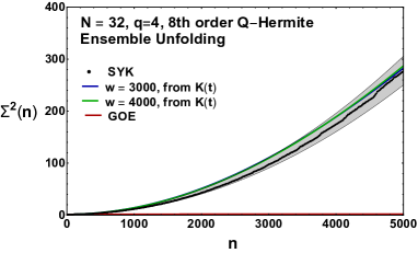
Figure 15: Number variances in the right figures are obtained from the spectral form factor in the left figures by evaluating the integral (131). The deviations in the number variance from the GOE result are due to the small $t$ peak in the spectral form factor.

In order to see the consistency of the calculation we compare two different ways to calculate the number variance: directly from eigenvalues and from using equation (131). The results are shown in figure 15. We conclude that a seemingly insignificant deviation of the form factor from the GOE result gives rise to a large deviation from the random matrix result for the $\bar{n}$-dependence of the number variance.

8 Double-trace moments and the validity of random matrix correlations

In this section we explore the question whether double-trace moments can shed light on the convergence to random matrix correlations. In subsection 8.1 we discuss the calculation of high-order double-trace moments, and in section 8.2 we evaluate the subleading corrections to estimate the convergence to the RMT result.

8.1 The calculation of high-order moments

The connected two-point correlator is given by

$$\langle\rho(x)\rho(y)\rangle_{c}=\frac{1}{4\pi^{2}}\int_{-\infty}^{\infty}\int_{-\infty}^{\infty}dsdte^{-ixs}e^{-iyt}\sum_{m,n}\frac{(it)^{m}(is)^{n}}{m!n!}\left(\tilde{M}_{m,n}-\tilde{M}_{m}\tilde{M}_{n}\right)$$ (134)

Since the universal random matrix result scales as

$$\frac{1}{D^{2}(x-y)^{2}},$$ (135)

high-order moments have to be suppressed by $2^{N}$, yet a naive subscripts counting when Wick-contracting $\Gamma$’s would suggest double traces are suppressed by a power law $N^{-kq}$ where $k$ is the number of cross links.

An important observation was first made in the appendix F of Cotler2016 on the nested cross-linked-only chord diagrams. The authors of Cotler2016 proved that

$$\begin{split}t_{1234\ldots k|k(k-1)\ldots 1}:\!&=2^{-N}\binom{N}{q}^{-k}\sum_{a_{1}\ldots a_{k}}\textrm{Tr}\left(\Gamma_{a_{1}}\Gamma_{a_{2}}\ldots\Gamma_{a_{k}}\right)\textrm{Tr}\left(\Gamma_{a_{k}}\Gamma_{a_{k-1}}\ldots\Gamma_{a_{1}}\right)\\ &=2^{-N}\sum_{m=0}^{N}\binom{N}{m}T_{m}(N,q)^{k},\end{split}$$ (136)

where $T_{m}$ was first defined in equation (34):

$$T_{m}:=\binom{N}{q}^{-1}\sum_{p=0}^{q}\binom{m}{p}\binom{N-m}{q-p}(-1)^{p}.$$

The observation was that

$$\lim_{k\to\infty}t_{1234\ldots k|k(k-1)\ldots 1}=2^{1-N}$$ (137)

for the simple reason that this limit is dominated by only two terms $m=0,N$, both of which give $T_{m}=1$ (other terms have $|T_{m}|<1$). This shows the naive expectation for moments is wrong and may serve as a starting point for understanding the RMT ramp from a moment method perspective.

In this section we offer a proof of a generalized version of equation (136), and in turn offer an interesting generalization of the limiting scenario (137).

The starting point of our proof is the completeness relation

$$2^{-N/2}\sum_{\mu}\left(X_{\mu}\right)_{ij}\left(X_{\mu}\right)_{kl}=\delta_{il}\delta_{jk}.$$ (138)

The $X_{\mu}$’s are as defined at the beginning of section 5: $\{X_{\mu}\}$ is the set of all linearly independent matrices formed by products of Dirac gamma matrices, with appropriate prefactors such that $X_{\mu}^{2}=\mathbb{1}$, and $\mu$ is a multi-index containing all the subscripts of the Dirac matrices in the product. The set $\{X_{\mu}\}$ has $2^{N}$ elements because they form a basis for the vector space of $2^{N/2}\times 2^{N/2}$ matrices. It will be useful to organize $X_{\mu}$’s by the number of Dirac matrices in the product, that is, the length $|\mu|$ of the multi-index $\mu$, then the completeness relation can be rewritten as

$$2^{-N/2}\sum_{m=0}^{N}\sum_{\mu_{m}}\left(X_{\mu_{m}}\right)_{ij}\left(X_{\mu_{m}}\right)_{kl}=\delta_{il}\delta_{jk},$$ (139)

where $\mu_{m}$ is a multi-index of length $m$, namely $|\mu_{m}|=m$.

Figure 16: Diagrammatic representation of equation (140). The dashed chord represents the inserted $X_{\mu_{m}}$. Chords can intersect in arbitrary ways in the shaded regions.

Inserting the completeness relation (138) in to double-trace moments, we have

$$\tilde{M}_{l,n}=2^{-N}\sum_{m=0}^{N}\sum_{\mu_{m}}\binom{N}{m}\frac{\langle\textrm{Tr}\left(X_{\mu_{m}}H^{l}X_{\mu_{m}}H^{n}\right)\rangle}{2^{N/2}\binom{N}{m}\sigma^{l+n}},$$ (140)

thus reducing every double trace to a sum over single traces. At the level of chord diagrams, this means every double-trace chord diagram can be written as a sum of single trace diagrams with one extra chord inserted, see figure 16 for illustration. From equation (140) we can further calculate each single trace by the combinatorics developed in Garcia-Garcia-ml-2018kvh , however, this does not warrant a straightforward application of the Q-Hermite approximation because this approximation has errors in polynomials of $1/N$, whereas the $\binom{N}{m}$ term is exponentially large in $N$ when $m\sim N/2$.

Let us calculate the contraction $t_{1234\ldots k|k(k-1)\ldots 1}$ which in terms of a single trace is given by

$$t_{1234\ldots k|k(k-1)\ldots 1}=2^{-N}\sum_{m=0}^{N}\binom{N}{m}\sum_{\mu_{m}}\sum_{a_{1},\ldots,a_{k}}\frac{\textrm{Tr}\left(X_{\mu_{m}}\Gamma_{a_{1}}\ldots\Gamma_{a_{k}}X_{\mu_{m}}\Gamma_{a_{k}}\ldots\Gamma_{a_{1}}\right)}{2^{N/2}\binom{N}{m}\binom{N}{q}^{k}}.$$ (141)

Since (with $c_{a\mu_{m}}$ the number of indices that $a$ and $\mu_{m}$ have in common)

$$X_{\mu_{m}}\Gamma_{a}=(-1)^{mq+c_{a\mu_{m}}}\Gamma_{a}X_{\mu_{m}},$$ (142)

we have for fixed $m$ that

$$\begin{split}\sum_{\mu_{m}}\sum_{a}\frac{\textrm{Tr}\left(X_{\mu_{m}}\Gamma_{a}X_{\mu_{m}}\Gamma_{a}\right)}{2^{N/2}\binom{N}{m}\binom{N}{q}}&=(-1)^{mq}\sum_{c_{a\mu_{m}}=0}^{q}\binom{m}{c_{a\mu_{m}}}\binom{N-m}{q-c_{a\mu_{m}}}(-1)^{c_{a\mu_{m}}}\\ &=(-1)^{mq}T_{m}.\end{split}$$ (143)

Substituting equation (143) into equation (141), we arrive at

$$t_{1234\ldots k|k(k-1)\ldots 1}=2^{-N}\sum_{m=0}^{N}\binom{N}{m}(-1)^{kmq}T_{m}^{k}.$$ (144)

This result is an application of the so-called “cut-vertex factorization” property for single traces Garcia-Garcia-ml-2018kvh . This property states that the chord intersections that do not form a closed loop factorize into products of individual intersections. In this instance we have $k$ independent intersections, each giving a factor of $(-1)^{mq}T_{m}$.

We thus have demonstrated that equation (140) reproduces equation (136) for even $q$ and even $k$, and trivially for when both $q$ and $k$ are odd because both formulas give zero. We will now use (140) to derive a modest generalization to equations (136) and (137). The diagrams we consider are the ones with a number of intersecting cross links and a number of nested links. Repeating the previous analysis, we conclude that these contributions are of the form

$$2^{-N}\sum_{m=0}^{N}\binom{N}{m}(-1)^{kmq}T_{m}^{k}\times\text{rest}(N,m,q),$$ (145)

where $k$ is the number of nested cross links and $\text{rest}(N,m,q)$ is whatever remains of the single-trace chord diagram after taking out the intersections between the dashed chord and nested links. We remind the reader that the dashed chord represents the insertion of $X_{\mu}$’s. Again in this limit the sum is dominated by two terms $m=0$ and $m=N$, so the limit is simply

$$2^{-N}\left[\text{rest}(N,0,q)+\text{rest}(N,N,q)\right].$$ (146)

Note that

$$\text{rest}(N,0,q)=\text{rest}(N,N,q)=\text{single-trace diagram with dashed chord removed},$$ (147)

because the $m=0$ and $m=N$ terms correspond to the insertions of identity matrix and Dirac chirality matrix in equation (140), and the chirality matrix insertion is equivalent to the identity matrix insertion when $q$ is even, we conclude that a diagram with a large number of nested cross links is equal to $2^{1-N}$ times the corresponding single-trace diagram with all nested links removed — see figure 17 for a concrete example.

The approach developed in this section can be viewed as complementary to that of section 6.1: the method of section 6.1 gives a completely combinatorial formula (103)–(106) in which the number of summations scales as a power in $q$ and is independent of $N$, hence is useful for calculating exact numerics for low-order moments with large $N$, as we have seen. However, for exactly the same reason it is not very useful for discussing the large $q$ behaviors, neither is it helpful for discussing the asymptotic behavior with large number of cross links due to its complexity. On the other hand, the approach of this section gives a symbolically simple formula in terms of single traces, hence makes various asymptotic behaviors amenable to discussion for a large number of nested cross links as we have seen and will see more soon.

Figure 17: An example of equation (146). The ellipses on the left represent infinite number of nested cross links. On the right we have same contraction with all the nested links removed, as a single trace diagram.

8.2 Long-wavelength fluctuations

Previously we saw a somewhat mysterious numerical phenomenon: we do not need to remove exponentially many long-range modes to get very close to the random matrix result. With the techniques discussed in section 8, we give a partial explanation to this phenomenon and estimate how the number of subtractions scales with $N$. We first summarize the gist of this section:

• The mode numbers correspond to the numbers of cross links in double-trace contractions.

• The double-trace contractions converge rapidly to the RMT result as the number of cross links increases.

Here by “RMT result” we simply mean the weak statement that after a certain point the contractions stop being suppressed by the number of cross links but by $2^{-N}$ instead, as would be the case for an RMT theory. As we have seen in equations (31) and (107), the double traces from diagrams with precisely two cross links can be entirely attributed to scale fluctuations — the lowest long-wavelength mode. For higher modes and larger number of cross links, we cannot make the correspondence as precise, but it is intuitively clear that both probe finer structures of the correlations. In the case of actual RMT ensembles, such a correspondence can be made precise brody1981 . Since the goal of this section is humble, this level of understanding should suffice as a starting point.

We will estimate speed of convergence of equation (137). In fact $t_{1234\ldots k|k(k-1)\ldots 1}$ is not quite the right quantity to study. Near equation (102), it was pointed out that for higher moments (large number of cross links) the contribution $\langle\textrm{Tr}\left(\gamma_{c}H^{m}\right)\left(\textrm{Tr}\gamma_{c}H^{n}\right)\rangle$ must be included. The completely nested diagram contribution in this double trace is

$$\begin{split}u_{1234\ldots k|k(k-1)\ldots 1}:\!&=2^{-N}\binom{N}{q}^{-k}\sum_{a_{1}\ldots a_{k}}\textrm{Tr}\left(\gamma_{c}\Gamma_{a_{1}}\Gamma_{a_{2}}\ldots\Gamma_{a_{k}}\right)\textrm{Tr}\left(\gamma_{c}\Gamma_{a_{k}}\Gamma_{a_{k-1}}\ldots\Gamma_{a_{1}}\right)\\ &=2^{-N}\sum_{m=0}^{N}\binom{N}{m}(-1)^{m}T_{m}^{k},\end{split}$$ (148)

where the second equality can again be proved by the insertion of completeness relation (138). Hence we have

$$t_{1234\ldots k|k(k-1)\ldots 1}+u_{1234\ldots k|k(k-1)\ldots 1}=2^{1-N}\sum_{m=0}^{N}\frac{1}{2}[1+(-1)^{m}]\binom{N}{m}T_{m}^{k},$$ (149)

and so we see only the even $m$ terms contribute. It is clear

$$\lim_{k\to\infty}[t_{1234\ldots k|k(k-1)\ldots 1}+u_{1234\ldots k|k(k-1)\ldots 1}]=2^{2-N},$$ (150)

and this is the quantity whose speed of convergence we wish to study. Its finite-$k$ relative deviation from the limiting result is

$$\frac{1}{2^{2-N}}\left(t_{1234\ldots k|k(k-1)\ldots 1}+u_{1234\ldots k|k(k-1)\ldots 1}\right)-1=\frac{1}{2}\sum_{m=2}^{N-2}\frac{1}{2}[1+(-1)^{m}]\binom{N}{m}T_{m}^{k}.$$ (151)

For $m\neq 0,N$, we have $|T_{m}|<1$, and the remaining largest terms are

$$T_{2}=T_{N-2}=1-\frac{4q}{N-1}+\frac{4q^{2}}{N(N-1)}.$$ (152)

So for large enough $k$, we would expect the summand $\binom{N}{m}T_{m}^{k}$ to be sharply peaked near $m=2,N-2$. Hence

$$\frac{1}{2}\sum_{m=2}^{N-2}\frac{1}{2}[1+(-1)^{m}]\binom{N}{m}T_{m}^{k}\approx\binom{N}{2}\left(1-\frac{4q}{N-1}+\frac{4q^{2}}{N(N-1)}\right)^{k}$$ (153)

So we see that contractions with $k>N/(2q)\log N$ are suppressed, and to obtain the RMT result we only have to subtract long wavelength fluctuations with $k<N/(2q)\log N$. For $N=32$ and $q=4$, we subtracted the first eight long-range modes to get a decent agreement to the RMT result, which is in the right ball park of our estimate $N/(2q)\log N\approx 14$. This analysis also applies to the slightly broader class of diagrams that include the ones described near equation (146).

For a more complete analysis, we would need to get a handle on the cases with linked intersections and the unfolding, which is outside the scope of this paper.

9 Discussion and conclusions

How can we analytically understand the observations of this paper? To get some perspective, we first discuss spectral correlations of the eigenvalues of the QCD Dirac operator. The first results were obtained in Halasz-ml-1995vd were the number variance was calculated from the quenched Dirac eigenvalues of a single lattice QCD configuration. Agreement with random matrix theory was found up to as many level spacings as allowed by the statistics (which is about 100 level spacings for a $12^{4}$ lattice). However, it was soon realized that when we compare to the ensemble average, which is what should be done, deviations are already visible on the scale of a couple of level spacings. The deviations are now well understood and can be obtained analytically from chiral perturbation theory Osborn-ml-1998qb ; BerbenniBitsch-ml-1999ti . The scale where deviations from random matrix theory occur is the quark mass scale for which the corresponding pion Compton wave length is equal to the size of the box.

The situation with the SYK model is similar. Comparing the estimate of the scale where spectral correlations start deviating from RMT with statistical fluctuations of the spectral density from one realization of the ensemble to the next, we see that the deviations from the RMT predictions can mostly be accounted for by such long-wavelength fluctuations. This is further confirmed by our numerical study, where after the first few long-wavelength modes are subtracted realization by realization of the ensemble, the spectral form factor becomes RMT-behaved until very short times and the number variance has RMT spectral rigidity until the energy scale given by the wavelength of the subtracted modes. This can be partly explained by the fact that the Hilbert space is $2^{N/2}$-dimensional whereas there are only $\binom{N}{q}$ model parameters $J_{\alpha}$, implying that very few matrix entries of the Hamiltonian can fluctuate independently. This scenario is to be contrasted with actual random matrix ensembles, where all matrix entries (barring Hermiticity and symmetry constraints) can fluctuate independently. However, this does not quite explain the separation of scales between the long-wavelength modes and scale of universal RMT fluctuations. We have gained some insight into this scale separation by looking at the convergence of a class of double-trace chord diagrams toward those of RMT, and analytically demonstrated that their early convergence behavior is consistent with our numerical results. It is desirable to have analytically controlled estimates of all chord diagrams to make more quantitative comparisons. We did develop a combinatorial formula for all chord diagrams in section 6.1, and it has been used to calculate the first few moments, but it is complicated and hard to apply to general high-order moments. We hope to investigate this in future works.

In the same vein of understanding QCD Dirac operator’s spectral statistics through chiral perturbation theory, we studied the nonlinear sigma model formulation of the spectral determinant of the SYK model. Although it is reassuring that the large energy expansion of the sigma model correctly reproduces the moments in a nontrivial manner, and that the wide correlator is given by the sum of the GUE result and corrections that are in agreement with numerical results, only few low-order correction terms could be calculated and it is not clear how the contribution of all other corrections to the two-point function cancels. In our view the following two issues have to be addressed to complete our understanding of the spectral density and spectral correlations in terms of the $\sigma$-model:

1. The most straightforward calculation gives a one-point resolvent that has the wrong branch cut. It is not known how to perform a resummation at the level of the $\sigma$-model action. In particular, we have not been able to obtain a Gaussian spectral density when $N\gg q$.

2. Although the correction terms to the RMT result explain the numerical results for $q=4$, it has not been shown that all other corrections in the loop expansion are small — in fact we do not know the range of validity of the loop expansion. Since naive application of the result to $q=2$, which has Poisson statistics, also gives RMT spectral correlations albeit with a much smaller Thouless energy, and we conclude that the loop expansion has to break down in this case.

Neither issue implies that the $\sigma$-model approach is inherently flawed, but they do suggest that our understanding of the $\sigma$-model is not complete. Similar issues arise in the calculation of nested cross-linked diagrams where the $q=2$ case is not qualitatively different from the $q=4$ case. We hope to address some of these questions in future work.

Appendix A Derivation of the $\sigma$-model

In this section we derive the nonlinear $\sigma$-model for the SYK model, see Verbaarschot1984 for the complex SYK model, and Altland-ml-2017eao for the Majorana SYK model. Our derivation follows a different route using the Fierz transformation, see also Liu-ml-2016rdi . Since $[\gamma_{c},H]=0$ we have the Hamiltonian in the block-diagonal form

$$H=\begin{pmatrix}H^{U}&\\ &H^{L}\end{pmatrix}=\sum_{\alpha}J_{\alpha}\Gamma_{\alpha}=\begin{pmatrix}\sum_{\alpha}J_{\alpha}\Gamma_{\alpha}^{U}&\\ &\sum_{\alpha}J_{\alpha}\Gamma_{\alpha}^{L}\end{pmatrix}$$ (154)

in the chiral basis where

$$\gamma_{c}=\text{diag}(\underbrace{1,\ldots,1}_{2^{N/2-1}},\underbrace{-1,\ldots,-1}_{2^{N/2-1}}).$$ (155)

Taking into account the unitary symmetries as required for universal RMT correlations, we focus on the upper block and define the generating function as

$$Z(x,y) =\left\langle{\det}^{-n}\left(x+H^{U}\right){\det}^{-n}\left(y+H^{U}\right)\right\rangle$$

$$=\left\langle\int\mathcal{D}\phi\mathcal{D}\phi^{*}e^{i\sum_{k}\phi_{1k}^{*}\cdot(x+H^{U})\cdot\phi_{1k}-i\sum_{k}\phi_{2k}^{*}\cdot(y+H^{U})\cdot\phi_{2k}}\right\rangle,$$ (156)

where $k$ is the replica index. We should think of $\phi$ as also having an implicit index of the $D=2^{N/2-1}$ dimensional Hilbert space (the index of the block Hamiltonian $H^{U}$) and “$\ \cdot\$” indicates summation over the Hilbert space index. The integrals are convergent because ${\rm Im}(x)=i\epsilon$ and ${\rm Im}(y)=-i\epsilon$. We also introduce the sign factor

$$\eta_{p}=(-1)^{p+1},$$ (157)

which will be inserted in the definition of the partition function such that the integrals are convergent. The correlation function of two resolvents is given by

$$\left\langle G(x)G(y)\right\rangle=\lim_{n\to 0}\frac{1}{n^{2}}\frac{1}{D^{2}}\frac{d}{dx}\frac{d}{dy}Z(x,y).$$ (158)

Recall that the disordered average is over Gaussian variables $J_{\alpha}$ with variance $v^{2}$, so after averaging we obtain

$$Z(x,y)=\int\mathcal{D}\phi e^{i\sum_{p,k}z_{pk}\eta_{p}\phi_{pk}^{*}\cdot\phi_{pk}-\frac{v^{2}}{2}\sum_{\alpha}\left(\sum_{p,k}\eta_{p}\phi^{*}_{pk}\cdot\left(\Gamma^{U}_{\alpha}\right)\cdot\phi_{pk}\right)^{2}},$$ (159)

where $p=1,2$, $k=1,2,\ldots,n$ and $z_{pk}$ can be viewed as the diagonal entries of

$$z:=\text{diag}(\overbrace{x,\cdots,x}^{n},\overbrace{y,\cdots,y}^{n})$$ (160)

defined in the replica space. Next we apply the Fierz transformation

$$\left(\Gamma_{\alpha}\right)_{ij}\left(\Gamma_{\alpha}\right)_{kl}=2^{-N}\sum_{\mu}\textrm{Tr}(\Gamma_{\alpha}X_{\mu}\Gamma_{\alpha}X_{\mu})\left(X_{\mu}\right)_{il}\left(X_{\mu}\right)_{kj},$$ (161)

where the $X_{\mu}$’s are defined in equation (138). Restricting this equation to the left-upper block, we get

$$\left(\Gamma^{U}_{\alpha}\right)_{ij}\left(\Gamma^{U}_{\alpha}\right)_{kl}=2^{1-N}\sum_{\mu,|\mu|\text{ even}}\textrm{Tr}(\Gamma^{U}_{\alpha}X^{U}_{\mu}\Gamma^{U}_{\alpha}X^{U}_{\mu})\left(X^{U}_{\mu}\right)_{il}\left(X^{U}_{\mu}\right)_{kj}.$$ (162)

We summed over $\mu$’s with even string length because only a product of even number of Dirac matrices has a non-zero left-upper block, and we denote the left-upper block of $X_{\mu}$ by ${X}^{U}_{\mu}$. We also used that

$$\textrm{Tr}(\Gamma_{\alpha}X_{\mu}\Gamma_{\alpha}X_{\mu})=2\textrm{Tr}\left(\Gamma^{U}_{\alpha}X^{U}_{\mu}\Gamma^{U}_{\alpha}X^{U}_{\mu}\right).$$ (163)

We can further reduce the number of generators in equation (162) by half by noticing that generators of $X_{\mu}$ with $|\mu|>N/2$ are related to $|\mu|<N/2$ one-to-one by multiplication of $\gamma_{c}$, and half of $X_{\mu}$’s with $|\mu|=N/2$ is related to the other half in the same way. On the other hand $\gamma_{c}$ is the identity matrix when restricted to upper block, so within the upper block the above-mentioned pairs are identical. This allows us to reduce the number of generators to $2^{N-2}=D^{2}$, and

$$\left(\Gamma^{U}_{\alpha}\right)_{ij}\left(\Gamma^{U}_{\alpha}\right)_{kl}=\frac{1}{D^{2}}\sum_{\mu}{}^{{}^{\prime}}\textrm{Tr}(\Gamma^{U}_{\alpha}X^{U}_{\mu}\Gamma^{U}_{\alpha}X^{U}_{\mu})\left(X^{U}_{\mu}\right)_{il}\left(X^{U}_{\mu}\right)_{kj},$$ (164)

where $\sum{}^{{}^{\prime}}_{\mu}$ denotes the sum over $\mu$’s with even $|\mu|$ and $|\mu|<N/2$ if $N/2$ is odd, and also over half of $\mu$’s with $|\mu|=N/2$ if $N/2$ is even. After the Fierz transformation we thus obtain the generating function

$$Z(x,y)=\int\mathcal{D}\phi\mathcal{D}\phi^{*}e^{i\sum_{p,k}\eta_{p}z_{pk}\phi_{pk}^{*}\cdot\phi_{pk}-\frac{\sigma^{2}}{2}\frac{1}{D}\sum_{pkql}\eta_{p}\eta_{q}\sum{}^{{}^{\prime}}_{\mu}T_{\mu}\phi^{*}_{pk}\cdot X^{U}_{\mu}\cdot\phi_{ql}\phi^{*}_{ql}\cdot X^{U}_{\mu}\cdot\phi_{pk}},$$ (165)

where $\sigma^{2}=\binom{N}{q}v^{2}$ is the multi-particle variance and

$$T_{\mu}=\frac{1}{D}\binom{N}{q}^{-1}\sum_{\alpha}\textrm{Tr}(\Gamma^{U}_{\alpha}X^{U}_{\mu}\Gamma^{U}_{\alpha}X^{U}_{\mu}).$$ (166)

Now we use that

$$\int da_{\mu}e^{-\frac{1}{2\sigma^{2}T_{\mu}}(a_{\mu}-i\sigma^{2}T_{\mu}\frac{1}{\sqrt{D}}\phi^{*}\cdot X^{U}_{\mu}\cdot\phi)^{2}}={\rm constant}.$$ (167)

This results in

$$Z(x,y)=\int\mathcal{D}a_{\mu}\mathcal{D}\phi\mathcal{D}\phi^{*}e^{i\sum_{pk}\eta_{p}z_{pk}\phi_{pk}^{*}\cdot\phi_{pk}}e^{-\sum{}^{{}^{\prime}}_{\mu}\frac{1}{2\sigma^{2}T_{\mu}}{\rm tr}a_{\mu}^{2}+\sum_{pkql}\eta_{p}\eta_{q}\sum{}^{{}^{\prime}}_{\mu}a_{\mu}^{pk;ql}i\frac{1}{\sqrt{D}}\phi_{pk}^{*}\cdot X^{U}_{\mu}\cdot\phi_{ql}}.$$ (168)

We can now perform the Gaussian integral over $\phi$ and $\phi^{*}$ resulting in the partition function

$$Z(x,y)=\int\mathcal{D}a_{\mu}e^{-\sum{}^{{}^{\prime}}_{\mu}\frac{1}{2\sigma^{2}T_{\mu}}{\rm tr}a_{\mu}^{2}-\textrm{Tr}\log(z+\sum{}^{{}^{\prime}}_{\mu}\frac{1}{\sqrt{D}}a_{\mu}X^{U}_{\mu})}.$$ (169)

A rescaling of the integration variable $a_{\mu}\to\sigma a_{\mu}$ gives equation (32). This is the partition function obtained by Altland and Bagrets Altland-ml-2017eao .

Note that the $\mu=0$ term in this sum is exactly the GUE result. This derivation raises an important concern. The $\mu=0$ term in (165) consists of $4n^{2}D^{2}{N\choose q}$ terms of the form $\phi^{i*}_{pk}\phi_{ql}^{i}\phi^{j*}_{ql}\phi_{pk}^{j}$ each with weight $\sigma^{2}/2D$. However, the expression before the Fierz transformation (159) has only $4n^{2}D{N/2\choose q}$ such terms from the diagonal $\Gamma^{\alpha}$ (there are ${N/2\choose q}$ of them) and $4n^{2}D\left[{N\choose q}-{N/2\choose q}\right]$ such terms from the off-diagonal $\Gamma^{\alpha}$, each with weight $\sigma^{2}/2$. Note that all $\Gamma^{\alpha}$ have only one nonzero matrix element in each column and in each row in the representation we are working in. So in total we have $4n^{2}D{N\choose q}$ terms of this form in equation (159) which is an exponentially smaller number than in equation (165), and most terms of the form $\phi^{i*}_{pk}\phi_{ql}^{i}\phi^{j*}_{ql}\phi_{pk}^{j}$ in (165) are actually canceled by the other terms obtained after the Fierz transformation. Indeed, the dominance of the GUE contribution has to break down for $q=2$, where the eigenvalues are uncorrelated. Yet, there is no qualitative difference between the $\sigma$-model for $q=2$ and $q=4$.

For $N\mod 8=0$ the $\gamma$ matrices are real and the spectral correlations are in the universality class of the Gaussian Orthogonal Ensemble (GOE). In this case, the term in (159)

$$\phi^{*}_{pk}\cdot\left(\Gamma^{U}_{\alpha}\right)\cdot\phi_{pk}$$ (170)

can be written as

$$\frac{1}{2}\left(\phi^{*}_{pk}\cdot\left(\Gamma^{U}_{\alpha}\right)\cdot\phi_{pk}+\phi_{pk}\cdot\left(\Gamma^{U}_{\alpha}\right)\cdot\phi^{*}_{pk}\right).$$ (171)

After applying the Fierz transformation, we obtain additional terms of the form

$$\sum_{pkql}\sum{}^{{}^{\prime}}_{\mu}T_{\mu}\phi^{*}_{pk}\cdot X^{U}_{\mu}\cdot\phi^{*}_{ql}\phi_{ql}\cdot X^{U}_{\mu}\cdot\phi_{pk},$$ (172)

which is the so-called Cooperon contribution to the GOE result. Note that in order to get a $\beta$-independent spectral density for the Wigner-Dyson ensemble, we have to scale the variance of the random matrix Hamiltonian as $1/\beta$. For the SYK model we do not have such rescaling and we expect an additional $\sqrt{\beta}$ dependence in the saddle-point equation and the corresponding resolvent and semi-circular spectral density.

Appendix B Some combinatorial identities

One can easily prove the identity

$$\frac{1}{D^{2}}\sum_{|\mu|=0}^{N}{N\choose|\mu|}T_{\mu}^{2}=4{N\choose q}^{-1}.$$ (173)

For arbitrary $p$ the sum behaves as

$$\frac{1}{D^{2}}\sum_{|\mu|=0}^{N}{N\choose|\mu|}T_{\mu}^{p}\sim N^{-qp/2}.$$ (174)

If $\nu$ is summed over with $|\nu|$ fixed we have

$$\frac{1}{D}\sum_{\nu,|\nu|{\rm fixed}}\textrm{Tr}X_{\mu}X_{\nu}X_{\mu}X_{\nu}=\sum_{s}(-1)^{s}{N\choose|\mu|}{N-|\mu|\choose|\nu|-s}{|\mu|\choose s}$$ (175)

Using this we obtain the identity

$$\frac{1}{D^{3}}\sum_{|\mu|=0}^{N}{N\choose|\mu|}\sum_{|\nu|=0}^{N}{N\choose|\nu|}\sum_{\nu}T_{\mu}^{p}T_{\nu}\textrm{Tr}X_{\mu}X_{\nu}X_{\mu}X_{\nu}=4\eta^{p},$$ (176)

which can also be shown by applying the Fierz transformation to $T_{\nu}X_{\nu}X_{\nu}$. To obtain the sixth moment from the $\sigma$-model calculation we need the identity

$$\sum_{m_{1}=0}^{N}\sum_{m_{2}=0}^{N}\sum_{s=0}^{m_{1}}{N\choose m_{1}}{m_{1}\choose s}{N-m_{1}\choose m_{2}-s}(-1)^{s}T_{m_{1}}T_{m_{2}}T_{m_{1}+m_{2}-2s}$$

$$=4{N\choose q}^{-2}\sum_{k=0}^{q}\sum_{m=0}^{q}(-1)^{q-k-m}{N-2k\choose q-m}{2k\choose m}{N-q\choose k}{q\choose k}.$$

$$\equiv 4T_{6}.$$ (177)

Here $T_{6}$ denotes the value of the single-trace diagram with three chords all intersecting with each other, see the footnote near the end of section 5.1.

Appendix C Replica limit of the GUE partition function

C.1 One-point function

The GUE partition function for $n$ replicas is given by

$$Z(z)=\int d\sigma\frac{1}{\det^{N}(z+\sigma)}e^{-\frac{N}{2}\sigma^{2}},$$ (178)

where the integral is over $n\times n$ Hermitian matrices $\sigma$. Using that the replica limit of the partition function is equal to one, we find that the resolvent is given by

$$G(z)=-\lim_{n\to 0}\frac{1}{n}\frac{1}{N}\frac{d}{dz}\log Z(z)=\lim_{n\to 0}\frac{1}{n}\int d\tilde{\sigma}{\rm tr}\tilde{\sigma}e^{-\frac{N}{2}\tilde{\sigma}^{2}-N{\rm tr}\log(z+\tilde{\sigma})},$$ (179)

where we have expressed the derivative with respect $z$ in terms of a derivative with respect to the $\tilde{\sigma}_{kk}$ and partially integrated these variables. We evaluate the resolvent in powers of $1/z$ and in powers of $1/N$. The saddle point equation is given by

$$\tilde{\sigma}+\frac{1}{\tilde{\sigma}+z}=0.$$ (180)

Expanding around the physical solution $\bar{\sigma}$ that asymptotes as $1/z$ for large $z$,

$$\tilde{\sigma}=\bar{\sigma}+\sigma,$$ (181)

and using the saddle point equation we obtain the expansion

$$G(z) =\bar{G}(z)+\lim_{n\to 0}\frac{1}{n}\int d\sigma{\rm tr}\sigma e^{-\frac{N}{2}(1-\bar{\sigma}^{2})\sigma^{2}+\sum_{k=3}^{\infty}\frac{1}{k}{\rm tr}\bar{\sigma}^{k}\sigma^{k}}$$

$$=\bar{G}(z)+\lim_{n\to 0}\frac{1}{n}\!\left(\!\frac{N}{3}\left\langle{\rm tr}\sigma{\rm tr}(\bar{\sigma}\sigma)^{3}\right\rangle+\frac{N}{5}\left\langle{\rm tr}\sigma{\rm tr}(\bar{\sigma}\sigma)^{5}\right\rangle+\frac{N}{7}\left\langle{\rm tr}\sigma{\rm tr}(\bar{\sigma}\sigma)^{7}\right\rangle+\frac{N}{9}\left\langle{\rm tr}\sigma{\rm tr}(\bar{\sigma}\sigma)^{9}\right\rangle\right.$$

$$\quad+\frac{N^{2}}{12}\left\langle{\rm tr}\sigma{\rm tr}(\bar{\sigma}\sigma)^{3}{\rm tr}(\bar{\sigma}\sigma)^{4}\right\rangle+\frac{N^{2}}{18}\left\langle{\rm tr}\sigma{\rm tr}(\bar{\sigma}\sigma)^{3}{\rm tr}(\bar{\sigma}\sigma)^{6}\right\rangle+\frac{N^{2}}{20}\left\langle{\rm tr}\sigma{\rm tr}(\bar{\sigma}\sigma)^{4}{\rm tr}(\bar{\sigma}\sigma)^{5}\right\rangle$$

$$\quad\left.+\frac{N^{3}}{162}\left\langle{\rm tr}\sigma({\rm tr}(\bar{\sigma}\sigma)^{3})^{3}\right\rangle\right)+\cdots,$$ (182)

where the expectation values are given by the sum over all corresponding Wick contractions. The terms with an odd number of factors of $\sigma$ vanish and we have not included them in the above. One can easily show that the following terms vanish in the replica limit

$$\lim_{n\to 0}\frac{1}{n}\left\langle{\rm tr}\sigma{\rm tr}\sigma^{3}\right\rangle =0,$$

$$\lim_{n\to 0}\frac{1}{n}\left\langle{\rm tr}\sigma{\rm tr}\sigma^{7}\right\rangle =0,$$

$$\lim_{n\to 0}\frac{1}{n}\left\langle{\rm tr}\sigma{\rm tr}\sigma^{3}{\rm tr}\sigma^{6}\right\rangle =0,$$

$$\lim_{n\to 0}\frac{1}{n}\left\langle{\rm tr}\sigma{\rm tr}\sigma^{4}{\rm tr}\sigma^{5}\right\rangle =0.$$ (183)

This leaves us with the following nonvanishing contributions

$$A_{1} =\lim_{n\to 0}\frac{1}{n}\frac{N}{5}\left\langle{\rm tr}\sigma{\rm tr}(\bar{\sigma}\sigma)^{5}\right\rangle=\frac{1}{N^{2}}\frac{\bar{\sigma}^{5}}{(1-\bar{\sigma}^{2})^{3}}=\frac{1}{N^{2}}\left[\frac{1}{z^{5}}+8\frac{1}{z^{7}}+47\frac{1}{z^{9}}+\cdots\right],$$

$$A_{2} =\lim_{n\to 0}\frac{1}{n}\frac{N}{9}\left\langle{\rm tr}\sigma{\rm tr}(\bar{\sigma}\sigma)^{9}\right\rangle=\frac{21}{N^{4}}\frac{\bar{\sigma}^{9}}{(1-\bar{\sigma}^{2})^{5}}=\frac{21}{N^{4}}\frac{1}{z^{9}},$$

$$A_{3} =\lim_{n\to 0}\frac{1}{n}\frac{N^{2}}{12}\left\langle{\rm tr}\sigma{\rm tr}(\bar{\sigma}^{3}\sigma)^{3}\textrm{Tr}(\bar{\sigma}\sigma)^{4}\right\rangle=\frac{1}{N^{2}}\frac{\bar{\sigma}^{7}}{(1-\bar{\sigma}^{2})^{4}}=\frac{1}{N^{2}}\left[\frac{1}{z^{7}}+11\frac{1}{z^{9}}+\cdots\right],$$

$$A_{4} =\lim_{n\to 0}\frac{1}{n}\frac{N^{2}}{12}\left\langle{\rm tr}\sigma{\rm tr}(\bar{\sigma}\sigma)^{3}\textrm{Tr}(\bar{\sigma}\sigma)^{4}\right\rangle=\frac{1}{N^{2}}\frac{\bar{\sigma}^{7}}{(1-\bar{\sigma}^{2})^{3}}=\frac{1}{N^{2}}\left[\frac{1}{z^{7}}+11\frac{1}{z^{9}}+\cdots\right],$$

$$A_{6} =\lim_{n\to 0}\frac{1}{n}\frac{N^{3}}{162}\left\langle{\rm tr}\sigma({\rm tr}(\bar{\sigma}\sigma)^{3})^{3}\right\rangle=\frac{1}{N^{2}}\frac{\bar{\sigma}^{9}}{(1-\bar{\sigma}^{2})^{5}}=\frac{1}{N^{2}}\left[\frac{1}{z^{9}}+\cdots\right].$$ (184)

A few comments on the evaluation of the contractions are in order. In total $9\times 105$ different diagrams contribute to $\langle{\rm tr}\sigma{\rm tr}\sigma^{9}\rangle$ but only $9\times 21$ of them do not vanish in the replica limit. The expression for $A_{3}$ and $A_{4}$ correspond to two different contraction patterns, namely,

$$\mathchoice{\vbox{\hbox to0.0pt{\kern 7.80557pt\kern 2.85706pt\hbox{\vrule width=0.50003pt,height=0.0pt,depth=4.30554pt\vrule width=13.5197pt,height=0.0pt,depth=0.50003pt\vrule width=0.50003pt,height=0.0pt,depth=4.30554pt}\hss}\vskip 2.15277pt\vskip 4.30554pt}}{\vbox{\hbox to0.0pt{\kern 7.80557pt\kern 2.85706pt\hbox{\vrule width=0.50003pt,height=0.0pt,depth=4.30554pt\vrule width=13.5197pt,height=0.0pt,depth=0.50003pt\vrule width=0.50003pt,height=0.0pt,depth=4.30554pt}\hss}\vskip 2.15277pt\vskip 4.30554pt}}{\vbox{\hbox to0.0pt{\kern 5.4639pt\kern 1.99994pt\hbox{\vrule width=0.50003pt,height=0.0pt,depth=4.30554pt\vrule width=9.46379pt,height=0.0pt,depth=0.50003pt\vrule width=0.50003pt,height=0.0pt,depth=4.30554pt}\hss}\vskip 2.15277pt\vskip 3.01389pt}}{\vbox{\hbox to0.0pt{\kern 3.90277pt\kern 1.42853pt\hbox{\vrule width=0.50003pt,height=0.0pt,depth=4.30554pt\vrule width=6.75983pt,height=0.0pt,depth=0.50003pt\vrule width=0.50003pt,height=0.0pt,depth=4.30554pt}\hss}\vskip 2.15277pt\vskip 2.15277pt}}\mathchoice{\vbox{\hbox to0.0pt{\kern 27.0394pt\kern 2.85706pt\hbox{\vrule width=0.50003pt,height=0.0pt,depth=8.61108pt\vrule width=19.23383pt,height=0.0pt,depth=0.50003pt\vrule width=0.50003pt,height=0.0pt,depth=8.61108pt}\hss}\vskip 2.15277pt\vskip 4.30554pt}}{\vbox{\hbox to0.0pt{\kern 27.0394pt\kern 2.85706pt\hbox{\vrule width=0.50003pt,height=0.0pt,depth=8.61108pt\vrule width=19.23383pt,height=0.0pt,depth=0.50003pt\vrule width=0.50003pt,height=0.0pt,depth=8.61108pt}\hss}\vskip 2.15277pt\vskip 4.30554pt}}{\vbox{\hbox to0.0pt{\kern 18.92758pt\kern 1.99994pt\hbox{\vrule width=0.50003pt,height=0.0pt,depth=8.61108pt\vrule width=13.46368pt,height=0.0pt,depth=0.50003pt\vrule width=0.50003pt,height=0.0pt,depth=8.61108pt}\hss}\vskip 2.15277pt\vskip 3.01389pt}}{\vbox{\hbox to0.0pt{\kern 13.51965pt\kern 1.42853pt\hbox{\vrule width=0.50003pt,height=0.0pt,depth=8.61108pt\vrule width=9.61688pt,height=0.0pt,depth=0.50003pt\vrule width=0.50003pt,height=0.0pt,depth=8.61108pt}\hss}\vskip 2.15277pt\vskip 2.15277pt}}\mathchoice{\vbox{\hbox to0.0pt{\kern 32.75352pt\kern 2.85706pt\hbox{\vrule width=0.50003pt,height=0.0pt,depth=12.91663pt\vrule width=24.94795pt,height=0.0pt,depth=0.50003pt\vrule width=0.50003pt,height=0.0pt,depth=12.91663pt}\hss}\vskip 2.15277pt\vskip 4.30554pt}}{\vbox{\hbox to0.0pt{\kern 32.75352pt\kern 2.85706pt\hbox{\vrule width=0.50003pt,height=0.0pt,depth=12.91663pt\vrule width=24.94795pt,height=0.0pt,depth=0.50003pt\vrule width=0.50003pt,height=0.0pt,depth=12.91663pt}\hss}\vskip 2.15277pt\vskip 4.30554pt}}{\vbox{\hbox to0.0pt{\kern 22.92747pt\kern 1.99994pt\hbox{\vrule width=0.50003pt,height=0.0pt,depth=12.91663pt\vrule width=17.46358pt,height=0.0pt,depth=0.50003pt\vrule width=0.50003pt,height=0.0pt,depth=12.91663pt}\hss}\vskip 2.15277pt\vskip 3.01389pt}}{\vbox{\hbox to0.0pt{\kern 16.37671pt\kern 1.42853pt\hbox{\vrule width=0.50003pt,height=0.0pt,depth=12.91663pt\vrule width=12.47394pt,height=0.0pt,depth=0.50003pt\vrule width=0.50003pt,height=0.0pt,depth=12.91663pt}\hss}\vskip 2.15277pt\vskip 2.15277pt}}\mathchoice{\vbox{\hbox to0.0pt{\kern 51.98735pt\kern 2.85706pt\hbox{\vrule width=0.50003pt,height=0.0pt,depth=17.22217pt\vrule width=11.42825pt,height=0.0pt,depth=0.50003pt\vrule width=0.50003pt,height=0.0pt,depth=17.22217pt}\hss}\vskip 2.15277pt\vskip 4.30554pt}}{\vbox{\hbox to0.0pt{\kern 51.98735pt\kern 2.85706pt\hbox{\vrule width=0.50003pt,height=0.0pt,depth=17.22217pt\vrule width=11.42825pt,height=0.0pt,depth=0.50003pt\vrule width=0.50003pt,height=0.0pt,depth=17.22217pt}\hss}\vskip 2.15277pt\vskip 4.30554pt}}{\vbox{\hbox to0.0pt{\kern 36.39116pt\kern 1.99994pt\hbox{\vrule width=0.50003pt,height=0.0pt,depth=17.22217pt\vrule width=7.99979pt,height=0.0pt,depth=0.50003pt\vrule width=0.50003pt,height=0.0pt,depth=17.22217pt}\hss}\vskip 2.15277pt\vskip 3.01389pt}}{\vbox{\hbox to0.0pt{\kern 25.99359pt\kern 1.42853pt\hbox{\vrule width=0.50003pt,height=0.0pt,depth=17.22217pt\vrule width=5.71411pt,height=0.0pt,depth=0.50003pt\vrule width=0.50003pt,height=0.0pt,depth=17.22217pt}\hss}\vskip 2.15277pt\vskip 2.15277pt}}{\rm tr}\sigma{\rm tr}\sigma\sigma\sigma{\rm tr}\sigma\sigma\sigma\sigma$$ (185)

and

$$\mathchoice{\vbox{\hbox to0.0pt{\kern 7.80557pt\kern 2.85706pt\hbox{\vrule width=0.50003pt,height=0.0pt,depth=4.30554pt\vrule width=38.46765pt,height=0.0pt,depth=0.50003pt\vrule width=0.50003pt,height=0.0pt,depth=4.30554pt}\hss}\vskip 2.15277pt\vskip 4.30554pt}}{\vbox{\hbox to0.0pt{\kern 7.80557pt\kern 2.85706pt\hbox{\vrule width=0.50003pt,height=0.0pt,depth=4.30554pt\vrule width=38.46765pt,height=0.0pt,depth=0.50003pt\vrule width=0.50003pt,height=0.0pt,depth=4.30554pt}\hss}\vskip 2.15277pt\vskip 4.30554pt}}{\vbox{\hbox to0.0pt{\kern 5.4639pt\kern 1.99994pt\hbox{\vrule width=0.50003pt,height=0.0pt,depth=4.30554pt\vrule width=26.92737pt,height=0.0pt,depth=0.50003pt\vrule width=0.50003pt,height=0.0pt,depth=4.30554pt}\hss}\vskip 2.15277pt\vskip 3.01389pt}}{\vbox{\hbox to0.0pt{\kern 3.90277pt\kern 1.42853pt\hbox{\vrule width=0.50003pt,height=0.0pt,depth=4.30554pt\vrule width=19.23376pt,height=0.0pt,depth=0.50003pt\vrule width=0.50003pt,height=0.0pt,depth=4.30554pt}\hss}\vskip 2.15277pt\vskip 2.15277pt}}\mathchoice{\vbox{\hbox to0.0pt{\kern 21.32527pt\kern 2.85706pt\hbox{\vrule width=0.50003pt,height=0.0pt,depth=8.61108pt\vrule width=30.66208pt,height=0.0pt,depth=0.50003pt\vrule width=0.50003pt,height=0.0pt,depth=8.61108pt}\hss}\vskip 2.15277pt\vskip 4.30554pt}}{\vbox{\hbox to0.0pt{\kern 21.32527pt\kern 2.85706pt\hbox{\vrule width=0.50003pt,height=0.0pt,depth=8.61108pt\vrule width=30.66208pt,height=0.0pt,depth=0.50003pt\vrule width=0.50003pt,height=0.0pt,depth=8.61108pt}\hss}\vskip 2.15277pt\vskip 4.30554pt}}{\vbox{\hbox to0.0pt{\kern 14.92769pt\kern 1.99994pt\hbox{\vrule width=0.50003pt,height=0.0pt,depth=8.61108pt\vrule width=21.46347pt,height=0.0pt,depth=0.50003pt\vrule width=0.50003pt,height=0.0pt,depth=8.61108pt}\hss}\vskip 2.15277pt\vskip 3.01389pt}}{\vbox{\hbox to0.0pt{\kern 10.6626pt\kern 1.42853pt\hbox{\vrule width=0.50003pt,height=0.0pt,depth=8.61108pt\vrule width=15.331pt,height=0.0pt,depth=0.50003pt\vrule width=0.50003pt,height=0.0pt,depth=8.61108pt}\hss}\vskip 2.15277pt\vskip 2.15277pt}}\mathchoice{\vbox{\hbox to0.0pt{\kern 27.0394pt\kern 2.85706pt\hbox{\vrule width=0.50003pt,height=0.0pt,depth=12.91663pt\vrule width=30.66208pt,height=0.0pt,depth=0.50003pt\vrule width=0.50003pt,height=0.0pt,depth=12.91663pt}\hss}\vskip 2.15277pt\vskip 4.30554pt}}{\vbox{\hbox to0.0pt{\kern 27.0394pt\kern 2.85706pt\hbox{\vrule width=0.50003pt,height=0.0pt,depth=12.91663pt\vrule width=30.66208pt,height=0.0pt,depth=0.50003pt\vrule width=0.50003pt,height=0.0pt,depth=12.91663pt}\hss}\vskip 2.15277pt\vskip 4.30554pt}}{\vbox{\hbox to0.0pt{\kern 18.92758pt\kern 1.99994pt\hbox{\vrule width=0.50003pt,height=0.0pt,depth=12.91663pt\vrule width=21.46347pt,height=0.0pt,depth=0.50003pt\vrule width=0.50003pt,height=0.0pt,depth=12.91663pt}\hss}\vskip 2.15277pt\vskip 3.01389pt}}{\vbox{\hbox to0.0pt{\kern 13.51965pt\kern 1.42853pt\hbox{\vrule width=0.50003pt,height=0.0pt,depth=12.91663pt\vrule width=15.331pt,height=0.0pt,depth=0.50003pt\vrule width=0.50003pt,height=0.0pt,depth=12.91663pt}\hss}\vskip 2.15277pt\vskip 2.15277pt}}\mathchoice{\vbox{\hbox to0.0pt{\kern 32.75352pt\kern 2.85706pt\hbox{\vrule width=0.50003pt,height=0.0pt,depth=17.22217pt\vrule width=30.66208pt,height=0.0pt,depth=0.50003pt\vrule width=0.50003pt,height=0.0pt,depth=17.22217pt}\hss}\vskip 2.15277pt\vskip 4.30554pt}}{\vbox{\hbox to0.0pt{\kern 32.75352pt\kern 2.85706pt\hbox{\vrule width=0.50003pt,height=0.0pt,depth=17.22217pt\vrule width=30.66208pt,height=0.0pt,depth=0.50003pt\vrule width=0.50003pt,height=0.0pt,depth=17.22217pt}\hss}\vskip 2.15277pt\vskip 4.30554pt}}{\vbox{\hbox to0.0pt{\kern 22.92747pt\kern 1.99994pt\hbox{\vrule width=0.50003pt,height=0.0pt,depth=17.22217pt\vrule width=21.46347pt,height=0.0pt,depth=0.50003pt\vrule width=0.50003pt,height=0.0pt,depth=17.22217pt}\hss}\vskip 2.15277pt\vskip 3.01389pt}}{\vbox{\hbox to0.0pt{\kern 16.37671pt\kern 1.42853pt\hbox{\vrule width=0.50003pt,height=0.0pt,depth=17.22217pt\vrule width=15.331pt,height=0.0pt,depth=0.50003pt\vrule width=0.50003pt,height=0.0pt,depth=17.22217pt}\hss}\vskip 2.15277pt\vskip 2.15277pt}}{\rm tr}\sigma{\rm tr}\sigma\sigma\sigma{\rm tr}\sigma\sigma\sigma\sigma.$$ (186)

This result (184) for the moments is in agreement with the general formula obtained by Mehta Mehta-2004 (see also Witte-ml-2013cea )

$$M_{2p}=(2p-1)!!\sum_{j=0}^{p}{p\choose j}{N\choose j+1}2^{j},$$ (187)

by comparing to $M_{2p}/(NM_{2}^{p})$.

C.2 Two-point function

The generating function for the two-point function of the GUE is given by

$$Z(z)=\int d\sigma\frac{1}{\det^{N}(z+\sigma)}e^{-\frac{N}{2}\sigma^{2}},$$ (188)

with $\sigma$ a Hermitian $2n\times 2n$ matrix and $z=\underbrace{(x,\cdots,x}_{n},\underbrace{y,\cdots,y}_{n})$. The corresponding blocks of the $\sigma$ matrix are referred to as the 11 block, the 12 block, the 21 block and the 22 block. For $x=y$ and both with the same infinitesimal increment, this becomes the generating function for the one-point function but now with $2n$ replicas. Note that for the two-point function, $x$ and $y$ have an opposite infinitesimal imaginary part, while for the one-point function, the imaginary parts of all $z$ have the same sign.

The two-point correlation function is given by

$$C(x,y) =\left.\lim_{n\to 0}\frac{1}{n^{2}N^{2}}\frac{d}{dx}\frac{d}{dy}\log Z(z)\right|_{\rm connected},$$

$$=\lim_{n\to 0}\frac{1}{n^{2}}\int d\sigma{\rm tr}P_{11}\sigma{\rm tr}P_{22}\sigma\frac{1}{\det^{N}(z+\sigma)}e^{-\frac{N}{2}\sigma^{2}}$$ (189)

with $P_{kk}$ the projection on the $kk$ block. The differentiation gives other contributions but they do not contribute to the connected two-point function. We evaluate the integral by a saddle point approximation. The saddle point equation is given by

$$\frac{1}{z+\sigma}+\sigma=0.$$ (190)

In a 12 block notation, the solution with $\sigma_{12}=0$ has the replica-diagonal form

$$\bar{\sigma}=\left(\begin{array}[]{cc}\bar{\sigma}(x)&0\\ 0&\bar{\sigma}(y)\end{array}\right).$$ (191)

The propagators and the vertices follow from the expansion of the logarithm

$$-{\rm tr}\log(z+\sigma)=\sum_{k=1}^{\infty}\frac{1}{k}(\bar{\sigma}\sigma)^{k}.$$ (192)

This results in the following quadratic part of the action

$$-\frac{N}{2}\left[(1-\bar{\sigma}(x)^{2}){\rm tr}\sigma_{11}^{2}+(1-\bar{\sigma}(y)^{2})\textrm{Tr}\sigma_{22}^{2}+2(1-\bar{\sigma}(x)\bar{\sigma}(y)){\rm tr}\sigma_{12}\sigma_{21}\right].$$ (193)

To leading order in $1/N^{2}$ two diagrams contribute to the two-point function:

$$\lim_{n\to 0}\frac{1}{n^{2}N^{2}}\left\langle{\rm tr}P_{11}\sigma{\rm tr}P_{22}\sigma\frac{1}{4}{\rm tr}(\bar{\sigma}\sigma)^{4}\right\rangle,$$ (194)

and

$$\lim_{n\to 0}\frac{1}{n^{2}N^{2}}\left\langle{\rm tr}P_{11}\sigma{\rm tr}P_{22}\sigma\frac{1}{18}{\rm tr}^{2}(\bar{\sigma}\sigma)^{3}\right\rangle.$$ (195)

The connected part of the first diagram is given by

$$\lim_{n\to 0}\frac{1}{n^{2}N^{2}}\left\langle{\rm tr}\sigma_{11}{\rm tr}\sigma_{22}{\rm tr}\sigma_{11}\sigma_{12}\sigma_{22}\sigma_{21}\right\rangle_{c}$$

$$=\frac{1}{N^{2}}\frac{(\bar{\sigma}(x)\bar{\sigma}(y))^{2}}{(1-\bar{\sigma}(x)\bar{\sigma}(y))(1-\bar{\sigma}^{2}(x))(1-\bar{\sigma}^{2}(x))}$$

$$=\frac{1}{N^{2}}\left(\frac{1}{x^{2}y^{2}}+\frac{1}{x^{3}y^{3}}+\cdots\right).$$ (196)

The connect part of the second diagram can be evaluated as

$$\lim_{n\to 0}\frac{1}{n^{2}N^{2}}\left\langle{\rm tr}\sigma_{11}{\rm tr}\sigma_{22}{\rm tr}\sigma_{11}\sigma_{12}\sigma_{21}{\rm tr}\sigma_{22}\sigma_{21}\sigma_{12}\right\rangle_{c}$$

$$=\frac{1}{N^{2}}\frac{(\bar{\sigma}(x)\bar{\sigma}(y))^{3}}{(1-\bar{\sigma}(x)\bar{\sigma}(y))^{2}(1-\bar{\sigma}^{2}(x))(1-\bar{\sigma}^{2}(x))}$$

$$=\frac{1}{N^{2}}\left(\frac{1}{x^{3}y^{3}}+\cdots\right).$$ (197)

The sum of the two contributions is equal to

$$=\frac{1}{N^{2}}\frac{(\bar{\sigma}(x)\bar{\sigma}(y))^{2}}{(1-\bar{\sigma}(x)\bar{\sigma}(y))^{2}(1-\bar{\sigma}^{2}(x))(1-\bar{\sigma}^{2}(x))}$$

$$=\frac{1}{N^{2}}\left(\frac{1}{x^{2}y^{2}}+\frac{2}{x^{3}y^{3}}+\cdots\right),$$ (198)

which gives the correct result for two-point correlator to order $1/N^{2}$ (see Verbaarschot1984 ) and the $M_{1,1}$ and $M_{2,2}$ moments. Note that in the normalization of this appendix, $\bar{\sigma}(x)\bar{\sigma}(y)\to 1$ for $x\to y$, so that the two-point function behaves as $1/(N^{2}(x-y)^{2})$ in this limit.

Appendix D Illustration of (103)–(106) by 3-cross-linked examples

To illustrate the general prescription for the evaluation double-trace diagrams (see section 6.1) we work out two double-trace diagrams with three cross-links in this appendix.

The starting point is the fact that $2^{-N/2}\textrm{Tr}(\Gamma_{a_{1}}\Gamma_{a_{2}}\ldots\Gamma_{a_{m}})$ can only be $0$ or $\pm 1$. This implies

$$2^{-N}\textrm{Tr}(\Gamma_{a_{1}}\Gamma_{a_{2}}\ldots\Gamma_{a_{m}})\textrm{Tr}(\Gamma_{a_{m}}\Gamma_{a_{m-1}}\ldots\Gamma_{a_{1}})=2^{-N}|\textrm{Tr}(\Gamma_{a_{1}}\Gamma_{a_{2}}\ldots\Gamma_{a_{m}})|^{2}=0\text{ or }1.$$ (199)

This particular simplicity motivates us to shuffle the $\Gamma$’s to the above “canonical” ordering. The shuffling will introduce phase factors due to the relation

$$\Gamma_{\alpha}\Gamma_{\beta}=(-1)^{q+c_{\alpha\beta}}\Gamma_{\beta}\Gamma_{\alpha},$$ (200)

where $c_{\alpha\beta}=|\alpha\cap\beta|$ is the number of common elements in sets $\alpha$ and $\beta$. For example let us consider the contraction $\textrm{Tr}(\Gamma_{a_{1}}\Gamma_{a_{2}}\Gamma_{a_{3}})\textrm{Tr}(\Gamma_{a_{1}}\Gamma_{a_{3}}\Gamma_{a_{2}})$, the shuffling (see figure 18) will introduce a phase factor of $(-1)^{c_{a_{1}a_{2}}+c_{a_{1}a_{3}}}$, and hence

$$\sum_{a_{1},a_{2},a_{3}}\textrm{Tr}(\Gamma_{a_{1}}\Gamma_{a_{2}}\Gamma_{a_{3}})\textrm{Tr}(\Gamma_{a_{1}}\Gamma_{a_{3}}\Gamma_{a_{2}})=\sum_{a_{1},a_{2},a_{3}}(-1)^{c_{a_{1}a_{2}}+c_{a_{1}a_{3}}}|\textrm{Tr}(\Gamma_{a_{1}}\Gamma_{a_{2}}\Gamma_{a_{3}})|^{2}.$$ (201)

In fact in this particular case we can get rid of the phase factor by cyclically permuting the $\Gamma$’s in the second trace, so we must have

$$\sum_{a_{1},a_{2},a_{3}}(-1)^{c_{a_{1}a_{2}}+c_{a_{1}a_{3}}}|\textrm{Tr}(\Gamma_{a_{1}}\Gamma_{a_{2}}\Gamma_{a_{3}})|^{2}=\sum_{a_{1},a_{2},a_{3}}|\textrm{Tr}(\Gamma_{a_{1}}\Gamma_{a_{2}}\Gamma_{a_{3}})|^{2}.$$

However we want to illustrate a general point beyond this simple example, so we keep the phase factors in our discussion. We see in general each intersection among the chords introduces a phase factor of $(-1)^{q+c_{\alpha\beta}}$. We would still like to get rid of the trace in our equation (201) in favor of a purely combinatorial term, so that it can be effectively handled by computers. The key question is, when is $2^{-N}|\textrm{Tr}(\Gamma_{a_{1}}\Gamma_{a_{2}}\Gamma_{a_{3}})|^{2}$ equal to $0$ and when is it equal to $1$?

Figure 18: Shuffling a double trace to its canonical ordering (subscripts not summed over).

Recall that each $\Gamma$ is a product of $q$ different Dirac matrices. The necessary and sufficient condition for $\textrm{Tr}(\Gamma_{a_{1}}\Gamma_{a_{2}}\Gamma_{a_{3}})$ to be nonvanishing is that every one of the $N$ Dirac matrices occurs exactly even number (including zero) of times in the totality of $\Gamma_{a_{1}},\Gamma_{a_{2}}$ and $\Gamma_{a_{3}}$.

This suggests that a useful perspective will be provided by the $d$-variables: $d_{a_{i_{1}}a_{i_{2}}\ldots a_{i_{k}}}$ is the number of elements common and only common to the sets $a_{i_{1}},a_{i_{2}},\ldots,a_{i_{k}}$ (naturally, $i_{1},\ldots,i_{k}$ are all different from each other in this definition). In the case of three index sets ($k=3$), we have the $d$-variables $\{d_{a_{1}a_{2}},d_{a_{1}a_{3}},d_{a_{2}a_{3}},d_{a_{1}a_{2}a_{3}}\}$. There are also $\{d_{a_{1}},d_{a_{2}},d_{a_{3}}\}$ which count the number of subscripts that occur exactly once in only $a_{1},a_{2}$ or $a_{3}$, but they are not independent variables due to the constraint that each index set has $q$ elements. Both the $c$-variables ($c_{a_{i_{1}}a_{i_{2}}}$) and the $d$-variables have played an important role in calculating single-trace contractions, and the relations between them were discussed in Garcia-Garcia-ml-2018kvh . Here we cite one diagram that makes their relation clear, see figure 19:

$$\begin{split}c_{a_{1}a_{2}}&=d_{a_{1}a_{2}}+d_{a_{1}a_{2}a_{3}};\\ c_{a_{1}a_{3}}&=d_{a_{1}a_{3}}+d_{a_{1}a_{2}a_{3}};\\ c_{a_{2}a_{3}}&=d_{a_{2}a_{3}}+d_{a_{1}a_{2}a_{3}}.\end{split}$$ (202)

In general,

$$c_{a_{i_{1}}a_{i_{2}}}=d_{a_{i_{1}}a_{i_{2}}}+\sum_{i_{3}\notin\{i_{1},i_{2}\}}d_{a_{i_{1}}a_{i_{2}}a_{i_{3}}}+\sum_{i_{3},i_{4}\notin\{i_{1},i_{2}\}}d_{a_{i_{1}}a_{i_{2}}a_{i_{3}}a_{i_{4}}}+\cdots+\sum_{i_{3},\ldots,i_{k}\notin\{i_{1},i_{2}\}}d_{a_{i_{1}}a_{i_{2}}a_{i_{3}}\ldots a_{i_{k}}}.$$ (203)

We come back to the case of $|\textrm{Tr}(\Gamma_{a_{1}}\Gamma_{a_{2}}\Gamma_{a_{3}})|^{2}$. Here $d_{a_{1}a_{2}}$ counts the number of Dirac matrices of which the subscripts appear exactly in sets $a_{1}$ and $a_{2}$, no less and no more. So there the Dirac matrices appear exactly twice in the totality of $\Gamma_{a_{1}},\Gamma_{a_{2}}$ and $\Gamma_{a_{3}}$.

Figure 19: Venn diagrams with three index sets. Each index set is represented by a circle, containing $q$ elements. The box is the set of all possible values an index can take, which has cardinality $N$. The box is partitioned into eight regions. (Taken from Garcia-Garcia-ml-2018kvh .)

The same can be said about $d_{a_{1}a_{3}}$ and $d_{a_{2}a_{3}}$. The total number of Dirac matrices that appear exactly twice in the totality of $\Gamma_{a_{1}},\Gamma_{a_{2}},\Gamma_{a_{3}}$ is thus

$$d_{2}=d_{a_{1}a_{2}}+d_{a_{1}a_{3}}+d_{a_{2}a_{3}}.$$ (204)

On the other hand $d_{a_{1}a_{2}a_{3}}$ counts the number of Dirac matrices that appear exactly three times in the totality of $\Gamma_{a_{1}},\Gamma_{a_{2}},\Gamma_{a_{3}}$. Hence if $d_{a_{1}a_{2}a_{3}}\neq 0$, $|\textrm{Tr}(\Gamma_{a_{1}}\Gamma_{a_{2}}\Gamma_{a_{3}})|^{2}=0$. We also want to know how many Dirac matrices appear exactly once:

$$\begin{split}\text{Exactly once in $a_{1}:$}&\ d_{a_{1}}=q-d_{a_{1}a_{2}}-d_{a_{1}a_{3}}-d_{a_{1}a_{2}a_{3}};\\ \text{Exactly once in $a_{2}:$}&\ d_{a_{2}}=q-d_{a_{1}a_{2}}-d_{a_{2}a_{3}}-d_{a_{1}a_{2}a_{3}};\\ \text{Exactly once in $a_{3}:$}&\ d_{a_{3}}=q-d_{a_{1}a_{3}}-d_{a_{2}a_{3}}-d_{a_{1}a_{2}a_{3}}.\end{split}$$ (205)

And $|\textrm{Tr}(\Gamma_{a_{1}}\Gamma_{a_{2}}\Gamma_{a_{3}})|^{2}=0$ also if any of the $\{d_{a_{1}},d_{a_{2}},d_{a_{3}}\}$ is nonzero. Synthesizing everything discussed so far, we arrive at the formula

$$\begin{split}&2^{-N}\sum_{a_{1},a_{2},a_{3}}\textrm{Tr}(\Gamma_{a_{1}}\Gamma_{a_{2}}\Gamma_{a_{3}})\textrm{Tr}(\Gamma_{a_{1}}\Gamma_{a_{3}}\Gamma_{a_{2}})\\ &=2^{-N}\sum_{a_{1},a_{2},a_{3}}(-1)^{c_{a_{1}a_{2}}+c_{a_{1}a_{3}}}|\textrm{Tr}(\Gamma_{a_{1}}\Gamma_{a_{2}}\Gamma_{a_{3}})|^{2}\\ &=\sum_{d_{a_{1}a_{2}}=0}^{q}\sum_{d_{a_{1}a_{3}}=0}^{q}\sum_{d_{a_{2}a_{3}}=0}^{q}(-1)^{d_{a_{1}a_{2}}+d_{a_{1}a_{3}}}\frac{N!}{(N-3q+d_{2})!d_{a_{1}a_{2}}!d_{a_{1}a_{3}}!d_{a_{2}a_{3}}!}\\ &\quad\qquad\qquad\qquad\times\delta(q-d_{a_{1}a_{2}}-d_{a_{1}a_{3}})\delta(q-d_{a_{1}a_{2}}-d_{a_{2}a_{3}})\delta(q-d_{a_{1}a_{3}}-d_{a_{2}a_{3}}).\end{split}$$ (206)

Note for the second equality we replaced the sum over index sets $a_{1},a_{2},a_{3}$ by a sum over numbers $d_{a_{1}a_{2}},d_{a_{1}a_{3}},d_{a_{2}a_{3}}$. In principle there is also a sum over $d_{a_{1}a_{2}a_{3}}$, but we have argued only the $d_{a_{1}a_{2}a_{3}}=0$ case contributes. It is clear that in this case there is only one scenario where the three Kronecker $\delta$ constraint is satisfied:

$$d_{a_{1}a_{2}}=d_{a_{1}a_{3}}=d_{a_{2}a_{3}}=\frac{q}{2},$$ (207)

which implies

$$2^{-N}\sum_{a_{1},a_{2},a_{3}}(-1)^{c_{a_{1}a_{2}}+c_{a_{1}a_{3}}}|\textrm{Tr}(\Gamma_{a_{1}}\Gamma_{a_{2}}\Gamma_{a_{3}})|^{2}=\begin{cases}0\ \,\quad\qquad\qquad\qquad\text{for odd }q,\\ \frac{N!}{\left(N-\frac{3q}{2}\right)!\left(\left(\frac{q}{2}\right)!\right)^{3}}\qquad\text{for even }q.\end{cases}$$ (208)

In more general cases no such drastic simplification can be expected.

Figure 20: The single trace chord diagram that has the same intersection structure as that of figure 18, note here all chords are attached to a single backbone as opposed to two in figure 18.

It is instructive to contrast equation (206) with the single trace contraction that has the same intersection structure (figure 20), using the results of Garcia-Garcia-ml-2018kvh :

$$2^{-N}\sum_{\alpha_{1},\alpha_{2},\alpha_{3}}\textrm{Tr}(\Gamma_{\alpha_{1}}\Gamma_{\alpha_{2}}\Gamma_{\alpha_{3}}\Gamma_{\alpha_{1}}\Gamma_{\alpha_{3}}\Gamma_{\alpha_{2}})$$

$$=\sum_{\alpha_{1},\alpha_{2},\alpha_{3}}(-1)^{c_{\alpha_{1}\alpha_{2}}+c_{\alpha_{1}\alpha_{3}}}$$

$$=\sum_{d_{\alpha_{1}\alpha_{2}\alpha_{3}}}\sum_{d_{\alpha_{1}\alpha_{2}}}\sum_{d_{\alpha_{1}\alpha_{3}}}\sum_{d_{\alpha_{2}\alpha_{3}}}(-1)^{d_{\alpha_{1}\alpha_{2}}+d_{\alpha_{1}\alpha_{3}}}\frac{N!}{(N-3q+d_{2}+2d_{\alpha_{1}\alpha_{2}\alpha_{3}})!d_{\alpha_{1}\alpha_{2}}!d_{\alpha_{1}\alpha_{3}}!d_{\alpha_{2}\alpha_{3}}!}$$

$$\quad\qquad\qquad\times\frac{1}{d_{\alpha_{1}\alpha_{2}\alpha_{3}}!}\frac{1}{(q-d_{\alpha_{1}\alpha_{2}}-d_{\alpha_{1}\alpha_{3}}-d_{\alpha_{1}\alpha_{2}\alpha_{3}})!}\frac{1}{(q-d_{\alpha_{1}\alpha_{2}}-d_{\alpha_{2}\alpha_{3}}-d_{\alpha_{1}\alpha_{2}\alpha_{3}})!}$$

$$\quad\qquad\qquad\times\frac{1}{(q-d_{\alpha_{1}\alpha_{3}}-d_{\alpha_{2}\alpha_{3}}-d_{\alpha_{1}\alpha_{2}\alpha_{3}})!}.$$ (209)

How about cases with both single-trace links and cross links? Let us consider the example in figure 21, we would need to calculate

$$\begin{split}&2^{-N}\sum_{a_{1},a_{2},a_{3},\beta}\textrm{Tr}(\Gamma_{a_{1}}\Gamma_{a_{2}}\Gamma_{a_{3}})\textrm{Tr}(\Gamma_{a_{1}}\Gamma_{a_{3}}\Gamma_{\beta}\Gamma_{a_{2}}\Gamma_{\beta})\\ &=2^{-N}\sum_{a_{1},a_{2},a_{3},\beta}(-1)^{q+c_{a_{1}a_{2}}+c_{a_{1}a_{3}}+c_{a_{2}\beta}}|\textrm{Tr}(\Gamma_{a_{1}}\Gamma_{a_{2}}\Gamma_{a_{3}})|^{2}.\end{split}$$ (210)

Now the $d$-variables are

$$\{d_{a_{1}a_{2}},d_{a_{1}a_{3}},d_{a_{2}a_{3}},d_{a_{1}\beta},d_{a_{2}\beta},d_{a_{3}\beta},d_{a_{1}a_{2}a_{3}},d_{a_{1}a_{2}\beta},d_{a_{1}a_{3}\beta},d_{a_{2}a_{3}\beta},d_{a_{1}a_{2}a_{3}\beta}\}.$$ (211)

However the constraint of the sum on the right-hand side is still given by the Kronecker deltas arising from $|\textrm{Tr}(\Gamma_{a_{1}}\Gamma_{a_{2}}\Gamma_{a_{3}})|^{2}$, just as in equation (206), so we may say similar things about the conditions on the contributing summands:

Figure 21: A chord diagram with three cross links and one single-trace link.

the traces with Dirac matrices whose subscripts appear odd number of times in the totality of $a_{1},a_{2},a_{3}$ are vanishing. This means

$$d_{a_{1}\beta},d_{a_{2}\beta},d_{a_{3}\beta},d_{a_{1}a_{2}a_{3}},d_{a_{1}a_{2}a_{3}\beta}$$

must all be zero. So the list (211) is shortened to

$$\{d_{a_{1}a_{2}},d_{a_{1}a_{3}},d_{a_{2}a_{3}},d_{a_{1}a_{2}\beta},d_{a_{1}a_{3}\beta},d_{a_{2}a_{3}\beta}\}.$$ (212)

We still need to take into account the Dirac matrices whose subscripts only appear once exclusively in either $a_{1}$, $a_{2}$ or $a_{3}$, and they are counted respectively by

$$\begin{split}d_{a_{1}}&=q-d_{a_{1}a_{2}}-d_{a_{1}a_{3}}-d_{a_{1}a_{2}\beta}-d_{a_{1}a_{3}\beta},\\ d_{a_{2}}&=q-d_{a_{1}a_{2}}-d_{a_{2}a_{3}}-d_{a_{1}a_{2}\beta}-d_{a_{2}a_{3}\beta},\\ d_{a_{3}}&=q-d_{a_{1}a_{3}}-d_{a_{2}a_{3}}-d_{a_{2}a_{3}\beta}-d_{a_{1}a_{3}\beta}.\end{split}$$ (213)

So these must also be zero. We also have

$$\begin{split}c_{a_{1}a_{2}}&=d_{a_{1}a_{2}}+d_{a_{1}a_{2}\beta},\\ c_{a_{1}a_{3}}&=d_{a_{1}a_{3}}+d_{a_{1}a_{3}\beta},\\ c_{a_{2}\beta}&=d_{a_{1}a_{2}\beta}+d_{a_{2}a_{3}\beta}.\end{split}$$ (214)

We conclude then that equation (210) is equal to

$$\begin{split}&\sum_{d_{a_{1}a_{2}}}\sum_{d_{a_{1}a_{3}}}\sum_{d_{a_{2}a_{3}}}\sum_{d_{a_{1}a_{2}\beta}}\sum_{d_{a_{1}a_{3}\beta}}\sum_{d_{a_{2}a_{3}\beta}}(-1)^{q+d_{a_{1}a_{2}}+d_{a_{1}a_{3}}+d_{a_{1}a_{3}\beta}+d_{a_{2}a_{3}\beta}}\\ &\qquad\qquad\times\frac{N!}{(N-4q+d_{2}+2d_{3})!}\frac{1}{d_{a_{1}a_{2}}!d_{a_{1}a_{3}}!d_{a_{2}a_{3}}!d_{a_{1}a_{2}\beta}!d_{a_{1}a_{3}\beta}!d_{a_{2}a_{3}\beta}!}\\ &\qquad\qquad\times\delta(q-d_{a_{1}a_{2}}-d_{a_{1}a_{3}}-d_{a_{1}a_{2}\beta}-d_{a_{1}a_{3}\beta})\\ &\qquad\qquad\times\delta(q-d_{a_{1}a_{2}}-d_{a_{2}a_{3}}-d_{a_{1}a_{2}\beta}-d_{a_{2}a_{3}\beta})\\ &\qquad\qquad\times\delta(q-d_{a_{1}a_{3}}-d_{a_{2}a_{3}}-d_{a_{2}a_{3}\beta}-d_{a_{1}a_{3}\beta}),\end{split}$$ (215)

where

$$\begin{split}d_{2}&=d_{a_{1}a_{2}}+d_{a_{1}a_{3}}+d_{a_{2}a_{3}},\\ d_{3}&=d_{a_{1}a_{2}\beta}+d_{a_{1}a_{3}\beta}+d_{a_{2}a_{3}\beta}.\end{split}$$ (216)

These examples enable us to see how the general situation can be handled, which is summarized in equations (103)–(106).

Appendix E Low-order double-trace moments

Using the properties of double traces discussed so far, we can sort out the following few nontrivial low-order double-trace moments:

$$\tilde{M}_{3,3} =3\left(1+(-1)^{q(q-1)/2}\right)t_{123|321},$$ (217)

$$\tilde{M}_{4,4} =\tilde{M}_{4}^{2}+8\binom{N}{q}^{-1}\tilde{M}_{4}^{2}+8t_{1234|4321}+16t_{1234|3421},$$ (218)

$$\tilde{M}_{3,5} =15(1+\eta)\left(1+(-1)^{q(q-1)/2}\right)t_{123|321},$$ (219)

$$\tilde{M}_{4,6} =\tilde{M}_{4}\tilde{M}_{6}+12\binom{N}{q}^{-1}\tilde{M}_{4}\tilde{M}_{6}+6(1+\eta)\left(8t_{1234|4321}+16t_{1234|3421}\right)$$

$$\quad+24\left(t_{1234|43\alpha 21\alpha}+t_{1234|34\alpha 21\alpha}+t_{1234|42\alpha 31\alpha}\right),$$ (220)

$$\tilde{M}_{5,5} =75\left(1+(-1)^{q(q-1)/2}\right)(1+\eta)^{2}t_{123|321}+5\left(1+(-1)^{q(q-1)/2}\right)$$

$$\quad\qquad\quad\times\left(t_{12345|54321}+5t_{12345|45321}+5t_{12345|35421}+t_{12345|42531}\right),$$ (221)

$$\tilde{M}_{6,6} =\tilde{M}_{6}^{2}+18\binom{N}{q}^{-1}\tilde{M}_{6}^{2}+36(1+\eta)^{2}\left(8t_{1234|4321}+16t_{1234|3421}\right)$$

$$\quad+36\times 8(1+\eta)\left(t_{1234|43\alpha 21\alpha}+t_{1234|34\alpha 21\alpha}+t_{1234|42\alpha 31\alpha}\right)$$

$$\quad+36\left(t_{\alpha 12\alpha 34|43\beta 21\beta}+t_{\alpha 12\alpha 34|34\beta 21\beta}+t_{\alpha 12\alpha 34|42\beta 31\beta}\right.$$

$$\quad\qquad\qquad\qquad\qquad\quad\left.+2t_{\alpha 12\alpha 34|24\beta 31\beta}+t_{\alpha 12\alpha 34|23\beta 41\beta}\right)$$

$$\quad+12\left(t_{123456|654321}+6t_{123456|564321}+12t_{123456|465321}\right.$$

$$\quad\left.\qquad\qquad+3t_{123456|456321}+9t_{123456|563421}+12t_{123456|536421}\right.$$

$$\quad\left.\qquad\qquad\qquad+12t_{123456|356421}+2t_{123456|436521}+3t_{123456|462531}\right).$$ (222)

The $t$-variables with subscripts denote chord diagrams, whose meaning should be evident from the two examples in figure 22.

Figure 22: Definition of the $t$-variables.

We are interested in the case of $N=32$ and $q=4$ for comparison with the numerical results. Every term in these low-order double-trace moments can be calculated using the formulas developed in section 6.1. We only present the final values of these terms in the next subsection of this appendix.

E.1 Values for low-order double-trace contractions ($N=32,q=4$)

In this appendix we list the explicit values of the terms that appeared in the low-order double -trace moments. Some of the contributing terms are purely single-trace ($\eta,M_{4},M_{6}$), and are thoroughly discussed in Garcia-Garcia-ml-2018kvh :

$$\begin{split}\eta&=1191/4495,\\ \tilde{M}_{4}&=10181/4495,\\ \tilde{M}_{6}&=137227959/20205025.\end{split}$$ (223)

The rest of the terms are the connected double-trace contractions that can be calculated by the method laid out in section 6.1:

$$\begin{split}t_{123|321}&=567/323280400,\\ t_{1234|4321}&=7168277/23250326368000,\\ t_{1234|3421}&=-555243/23250326368000,\\ t_{1234|43\alpha 21\alpha}&=5928671067/104510217024160000,\\ t_{1234|34\alpha 21\alpha}&=518354267/104510217024160000,\\ t_{1234|42\alpha 31\alpha}&=-711893157/104510217024160000,\\ t_{12345|54321}&=8116630557/104510217024160000,\\ t_{12345|45321}&=-462480963/104510217024160000,\\ t_{12345|35421}&=160002717/104510217024160000,\\ t_{12345|42531}&=-6933507/104510217024160000,\\ t_{\alpha 12\alpha 34|43\beta 21\beta}&=7519992447797/469773425523599200000,\\ t_{\alpha 12\alpha 34|34\beta 21\beta}&=520655935797/469773425523599200000,\\ t_{\alpha 12\alpha 34|42\beta 31\beta}&=-368559700939/469773425523599200000,\\ t_{\alpha 12\alpha 34|24\beta 31\beta}&=120146887221/469773425523599200000,\\ t_{\alpha 12\alpha 34|23\beta 41\beta}&=4043901987381/469773425523599200000,\\ t_{123456|654321}&=6135081997081/234886712761799600000,\\ t_{123456|564321}&=-60665945079/234886712761799600000,\\ t_{123456|465321}&=-687382239/234886712761799600000,\\ t_{123456|456321}&=31234591/7576990734251600000,\\ t_{123456|563421}&=89686592361/234886712761799600000,\\ t_{123456|536421}&=3173529/234886712761799600000,\\ t_{123456|356421}&=-19709513199/234886712761799600000,\\ t_{123456|436521}&=5189715001/234886712761799600000,\\ t_{123456|462531}&=589707393/234886712761799600000.\end{split}$$ (224)

References

- (1)
- (2) A. Kitaev, A simple model of quantum holography, KITP strings seminar and Entanglement 2015 program, 12 February, 7 April and 27 May 2015 [http://online.kitp.ucsb.edu/online/entangled15/].
- (3) S. Sachdev and J. Ye, Gapless spin fluid ground state in a random, quantum Heisenberg magnet, Phys. Rev. Lett. 70 (1993) 3339 [cond-mat/9212030] [INSPIRE].
- (4) J. Maldacena and D. Stanford, Remarks on the Sachdev-Ye-Kitaev model, Phys. Rev. D 94 (2016) 106002 [arXiv:1604.07818] [INSPIRE].
- (5) L.V. Iliesiu, S.S. Pufu, H. Verlinde and Y. Wang, An exact quantization of Jackiw-Teitelboim gravity, JHEP 11 (2019) 091 [arXiv:1905.02726] [INSPIRE].
- (6) S. Sachdev, Holographic metals and the fractionalized Fermi liquid, Phys. Rev. Lett. 105 (2010) 151602 [arXiv:1006.3794] [INSPIRE].
- (7) S.H. Shenker and D. Stanford, Black holes and the butterfly effect, JHEP 03 (2014) 067 [arXiv:1306.0622] [INSPIRE].
- (8) J. Cotler and N. Hunter-Jones, Spectral decoupling in many-body quantum chaos, arXiv:1911.02026 [INSPIRE].
- (9) F. Borgonovi, F.M. Izrailev and L.F. Santos, Timescales in the quench dynamics of many-body quantum systems: Participation ratio versus out-of-time ordered correlator, Phys. Rev. E 99 (2019) 052143 [arXiv:1903.09175] [INSPIRE].
- (10) O. Bohigas, M.J. Giannoni and C. Schmit, Characterization of chaotic quantum spectra and universality of level fluctuation laws, Phys. Rev. Lett. 52 (1984) 1 [INSPIRE].
- (11) Y.-Z. You, A.W.W. Ludwig and C. Xu, Sachdev-Ye-Kitaev Model and Thermalization on the Boundary of Many-Body Localized Fermionic Symmetry Protected Topological States, Phys. Rev. B 95 (2017) 115150 [arXiv:1602.06964] [INSPIRE].
- (12) A.M. García-García and J.J.M. Verbaarschot, Spectral and thermodynamic properties of the Sachdev-Ye-Kitaev model, Phys. Rev. D 94 (2016) 126010 [arXiv:1610.03816] [INSPIRE].
- (13) J.S. Cotler et al., Black Holes and Random Matrices, JHEP 05 (2017) 118 [Erratum ibid. 09 (2018) 002] [arXiv:1611.04650] [INSPIRE].
- (14) P. Saad, S.H. Shenker and D. Stanford, A semiclassical ramp in SYK and in gravity, arXiv:1806.06840 [INSPIRE].
- (15) J.J.M Verbaarschot and M.R Zirnbauer, Replica variables, loop expansion and spectral rigidity of random-matrix ensembles, Annals Phys. 158 (1984) 78.
- (16) A. Altland and D. Bagrets, Quantum ergodicity in the SYK model, Nucl. Phys. B 930 (2018) 45 [arXiv:1712.05073] [INSPIRE].
- (17) A.M. García-García, Y. Jia and J.J.M. Verbaarschot, Universality and Thouless energy in the supersymmetric Sachdev-Ye-Kitaev Model, Phys. Rev. D 97 (2018) 106003 [arXiv:1801.01071] [INSPIRE].
- (18) H. Gharibyan, M. Hanada, S.H. Shenker and M. Tezuka, Onset of Random Matrix Behavior in Scrambling Systems, JHEP 07 (2018) 124 [Erratum ibid. 02 (2019) 197] [arXiv:1803.08050] [INSPIRE].
- (19) J.B. French and S.S.M. Wong, Some random-matrix level and spacing distributions for fixed-particle-rank interactions, Phys. Lett. B 35 (1971) 5 [INSPIRE].
- (20) O. Bohigas and J. Flores, Two-body random hamiltonian and level density, Phys. Lett. B 34 (1971) 261 [INSPIRE].
- (21) K. Mon and J.B. French, Statistical Properties of Many Particle Spectra, Annals Phys. 95 (1975) 90 [INSPIRE].
- (22) S. Sachdev, Bekenstein-Hawking Entropy and Strange Metals, Phys. Rev. X 5 (2015) 041025 [arXiv:1506.05111] [INSPIRE].
- (23) D. Bagrets, A. Altland and A. Kamenev, Sachdev-Ye-Kitaev model as Liouville quantum mechanics, Nucl. Phys. B 911 (2016) 191 [arXiv:1607.00694] [INSPIRE].
- (24) A.M. García-García and J.J.M. Verbaarschot, Analytical Spectral Density of the Sachdev-Ye-Kitaev Model at finite N, Phys. Rev. D 96 (2017) 066012 [arXiv:1701.06593] [INSPIRE].
- (25) D. Stanford and E. Witten, Fermionic Localization of the Schwarzian Theory, JHEP 10 (2017) 008 [arXiv:1703.04612] [INSPIRE].
- (26) H.A. Bethe, An Attempt to Calculate the Number of Energy Levels of a Heavy Nucleus, Phys. Rev. 50 (1936) 332 [INSPIRE].
- (27) E. Witten, An SYK-Like Model Without Disorder, J. Phys. A 52 (2019) 474002 [arXiv:1610.09758] [INSPIRE].
- (28) I.R. Klebanov and G. Tarnopolsky, Uncolored random tensors, melon diagrams and the Sachdev-Ye-Kitaev models, Phys. Rev. D 95 (2017) 046004 [arXiv:1611.08915] [INSPIRE].
- (29) J. Kim, I.R. Klebanov, G. Tarnopolsky and W. Zhao, Symmetry Breaking in Coupled SYK or Tensor Models, Phys. Rev. X 9 (2019) 021043 [arXiv:1902.02287] [INSPIRE].
- (30) I. Kourkoulou and J. Maldacena, Pure states in the SYK model and nearly- gravity, arXiv:1707.02325 [INSPIRE].
- (31) A. Almheiri, A. Milekhin and B. Swingle, Universal Constraints on Energy Flow and SYK Thermalization, arXiv:1912.04912 [INSPIRE].
- (32) J. Sonner and M. Vielma, Eigenstate thermalization in the Sachdev-Ye-Kitaev model, JHEP 11 (2017) 149 [arXiv:1707.08013] [INSPIRE].
- (33) A. del Campo, J. Molina-Vilaplana, L.F. Santos and J. Sonner, Decay of a Thermofield-Double State in Chaotic Quantum Systems, Eur. Phys. J. ST 227 (2018) 247 [arXiv:1709.10105] [INSPIRE].
- (34) T. Nosaka, D. Rosa and J. Yoon, The Thouless time for mass-deformed SYK, JHEP 09 (2018) 041 [arXiv:1804.09934] [INSPIRE].
- (35) A.M. García-García, B. Loureiro, A. Romero-Bermúdez and M. Tezuka, Chaotic-Integrable Transition in the Sachdev-Ye-Kitaev Model, Phys. Rev. Lett. 120 (2018) 241603 [arXiv:1707.02197] [INSPIRE].
- (36) J. Maldacena and X.-L. Qi, Eternal traversable wormhole, arXiv:1804.00491 [INSPIRE].
- (37) A.M. García-García, T. Nosaka, D. Rosa and J.J.M. Verbaarschot, Quantum chaos transition in a two-site Sachdev-Ye-Kitaev model dual to an eternal traversable wormhole, Phys. Rev. D 100 (2019) 026002 [arXiv:1901.06031] [INSPIRE].
- (38) K. Okuyama, Replica symmetry breaking in random matrix model: a toy model of wormhole networks, Phys. Lett. B 803 (2020) 135280 [arXiv:1903.11776] [INSPIRE].
- (39) G. Penington, S.H. Shenker, D. Stanford and Z. Yang, Replica wormholes and the black hole interior, arXiv:1911.11977 [INSPIRE].
- (40) J. Maldacena and A. Milekhin, SYK wormhole formation in real time, arXiv:1912.03276 [INSPIRE].
- (41) J. De Boer, R. Van Breukelen, S.F. Lokhande, K. Papadodimas and E. Verlinde, Probing typical black hole microstates, JHEP 01 (2020) 062 [arXiv:1901.08527] [INSPIRE].
- (42) A. Kruchkov, A. Patel, P. Kim and S. Sachdev, Thermoelectric power of Sachdev-Ye-Kitaev islands: Probing Bekenstein-Hawking entropy in quantum matter experiments, Phys. Rev. B 101 (2020) 205148 [arXiv:1912.02835] [INSPIRE].
- (43) A. Altland, D. Bagrets and A. Kamenev, Sachdev-Ye-Kitaev Non-Fermi-Liquid Correlations in Nanoscopic Quantum Transport, Phys. Rev. Lett. 123 (2019) 226801 [arXiv:1908.11351] [INSPIRE].
- (44) J.F. Karcher, M. Sonner and A.D. Mirlin, Disorder and interaction in chiral chains: Majoranas versus complex fermions, Phys. Rev. B 100 (2019) 134207 [arXiv:1905.12743] [INSPIRE].
- (45) Y. Gu, A. Kitaev, S. Sachdev and G. Tarnopolsky, Notes on the complex Sachdev-Ye-Kitaev model, JHEP 02 (2020) 157 [arXiv:1910.14099] [INSPIRE].
- (46) D. Rossini, G.M. Andolina, D. Rosa, M. Carrega and M. Polini, Quantum charging supremacy via Sachdev-Ye-Kitaev batteries, arXiv:1912.07234 [INSPIRE].
- (47) P. Saad, S.H. Shenker and D. Stanford, JT gravity as a matrix integral, arXiv:1903.11115 [INSPIRE].
- (48) D. Stanford and E. Witten, JT Gravity and the Ensembles of Random Matrix Theory, arXiv:1907.03363 [INSPIRE].
- (49) P. Saad, Late Time Correlation Functions, Baby Universes and ETH in JT Gravity, arXiv:1910.10311 [INSPIRE].
- (50) A.M. García-García and S. Zacarías, Quantum Jackiw-Teitelboim gravity, Selberg trace formula and random matrix theory, arXiv:1911.10493 [INSPIRE].
- (51) D.J. Gross, J. Kruthoff, A. Rolph and E. Shaghoulian, Hamiltonian deformations in quantum mechanics, and SYK, arXiv:1912.06132 [INSPIRE].
- (52) V. Oganesyan and D.A. Huse, Localization of interacting fermions at high temperature, Phys. Rev. B 75 (2007) 155111.
- (53) J.B. French, Analysis of distant-neighbor spacing distributions for k-body interaction ensembles, Rev. Mex. Fis. 22 (1973) 221.
- (54) J. Flores, M. Horoi, M. Müller and T.H. Seligman, Spectral statistics of the two-body random ensemble revisited, Phys. Rev. E 63 (2001) 026204 [cond-mat/0006144] [INSPIRE].
- (55) I.R. Klebanov, P.N. Pallegar and F.K. Popov, Majorana Fermion Quantum Mechanics for Higher Rank Tensors, Phys. Rev. D 100 (2019) 086003 [arXiv:1905.06264] [INSPIRE].
- (56) L. Benet and H.A. Weidenmüller, Review of the k body embedded ensembles of Gaussian random matrices, J. Phys. A 36 (2003) 3569 [cond-mat/0207656] [INSPIRE].
- (57) M. Srednicki, Spectral statistics of the k-body random-interaction model, Phys. Rev. E 66 (2002) 046138.
- (58) J.J.M. Verbaarschot and M.R. Zirnbauer, Critique of the Replica Trick, J. Phys. A 18 (1985) 1093 [INSPIRE].
- (59) H. Wang, D. Bagrets, A.L. Chudnovskiy and A. Kamenev, On the replica structure of Sachdev-Ye-Kitaev model, JHEP 09 (2019) 057 [arXiv:1812.02666] [INSPIRE].
- (60) I. Aref’eva, M. Khramtsov, M. Tikhanovskaya and I. Volovich, On replica-nondiagonal large saddles in the SYK model, EPJ Web Conf. 191 (2018) 06007 [INSPIRE].
- (61) I. Aref’eva, M. Khramtsov, M. Tikhanovskaya and I. Volovich, Replica-nondiagonal solutions in the SYK model, JHEP 07 (2019) 113 [arXiv:1811.04831] [INSPIRE].
- (62) M.E.H. Ismail, C. Stanton and G. Viennot, The Combinatorics of q-Hermite polynomials and the Askey-Wilson Integral, Eur. J. Combinatorics 8 (1987) 379.
- (63) A.M. García-García, Y. Jia and J.J.M. Verbaarschot, Exact moments of the Sachdev-Ye-Kitaev model up to order , JHEP 04 (2018) 146 [arXiv:1801.02696] [INSPIRE].
- (64) M. Berkooz, P. Narayan and J. Simon, Chord diagrams, exact correlators in spin glasses and black hole bulk reconstruction, JHEP 08 (2018) 192 [arXiv:1806.04380] [INSPIRE].
- (65) M. Berkooz, M. Isachenkov, V. Narovlansky and G. Torrents, Towards a full solution of the large double-scaled SYK model, JHEP 03 (2019) 079 [arXiv:1811.02584] [INSPIRE].
- (66) A. Cappelli and F. Colomo, Solving the frustrated spherical model with q polynomials, J. Phys. A 31 (1998) 3141 [hep-th/9710071] [INSPIRE].
- (67) Y. Jia and J.J.M. Verbaarschot, Large expansion of the moments and free energy of Sachdev-Ye-Kitaev model and the enumeration of intersection graphs, JHEP 11 (2018) 031 [arXiv:1806.03271] [INSPIRE].
- (68) A. Pandey, Statistical properties of many-particle spectra: III. ergodic behavior in random-matrix ensembles, Annals Phys. 118 (1979) 511.
- (69) A. Delon, R. Jost and M. Lombardi, NO2 jet cooled visible excitation spectrum-vibronic chaos induced by the - interaction, J. Chem. Phys. 95 (1991) 5701.
- (70) T.A. Brody, J. Flores, J.B. French, P.A. Mello, A. Pandey and S.S.M. Wong, Random matrix physics: Spectrum and strength fluctuations, Rev. Mod. Phys. 53 (1981) 385 [INSPIRE].
- (71) A.M. Halasz and J.J.M. Verbaarschot, Universal fluctuations in spectra of the lattice Dirac operator, Phys. Rev. Lett. 74 (1995) 3920 [hep-lat/9501025] [INSPIRE].
- (72) J.C. Osborn, D. Toublan and J.J.M. Verbaarschot, From chiral random matrix theory to chiral perturbation theory, Nucl. Phys. B 540 (1999) 317 [hep-th/9806110] [INSPIRE].
- (73) M.E. Berbenni-Bitsch et al., Random matrix theory, chiral perturbation theory and lattice data, Phys. Lett. B 466 (1999) 293 [hep-lat/9907014] [INSPIRE].
- (74) Y. Liu, M.A. Nowak and I. Zahed, Disorder in the Sachdev-Yee-Kitaev Model, Phys. Lett. B 773 (2017) 647 [arXiv:1612.05233] [INSPIRE].
- (75) M. Lal Mehta, Random Matrices, 3rd ed., Pure and Applied Mathematics, volume 142, Elsevier, Amsterdam (2004).
- (76) N.S. Witte and P.J. Forrester, Moments of the Gaussian Ensembles and the large- expansion of the densities, J. Math. Phys. 55 (2014) 083302 [arXiv:1310.8498] [INSPIRE].