We conduct a study of the aliased spectral densities of Matérn covariance functions on a regular grid of points, providing clarity on the properties of a popular approximation based on stochastic partial differential equations; while others have shown that it can approximate the covariance function well, we find that it assigns too much power at high frequencies and does not provide increasingly accurate approximations to the inverse as the grid spacing goes to zero, except in the one-dimensional exponential covariance case. We provide numerical results to support our theory, and in a simulation study, we investigate the implications for parameter estimation, finding that the SPDE approximation tends to overestimate spatial range parameters.

1 Introduction

The Matérn covariance between two points in $\mathbb{R}^{d}$ separated by lag $h\in\mathbb{R}^{d}$ is

$$M[\,h\,;\,\nu,d\,]=\frac{\sigma^{2}}{2^{\nu-1}\Gamma(\nu)}(\alpha\|h\|)^{\nu}K_{\nu}(\alpha\|h\|),$$ (1)

where $\sigma^{2}$ is a variance parameter, $\alpha$ is an inverse range parameter, $\nu$ is a smoothness parameter, and $K_{\nu}$ is the modified Bessel function of the second kind. Guttorp and Gneiting, (2006) provide a summary of its important properties and a detailed discussion of its history. Our article presents a theoretical and numerical study of properties of the spectral density of the Matérn covariance when aliased to regular grids of points in one and two dimensions. We apply our results to study a popular approximation to the inverse of Matérn covariance matrices that is motivated by connections between the Matérn covariance and a class of stochastic partial differential equations (SPDEs) (Lindgren et al.,, 2011).

Building on work by Whittle, (1954), Whittle, (1963), and Besag, (1981), Lindgren et al., (2011) proposed that the inverse of Matérn covariance matrices can be represented by sparse matrices whenever $\nu+d/2$ is an integer, which is why our notation for $M$ includes $\nu$ and $d$. The resulting approximation is commonly referred to as the SPDE approximation. In this paper, we use the terms “SPDE approach” and “SPDE approximation” to refer specificially to the methods in Lindgren et al., (2011). We investigate the sparsity of Matérn inverses and find that there is nothing particularly special with regards to sparsity about the $d=1,\nu=3/2$ case or the $d=2,\nu=1$ case, relative to other values of $\nu$. Further, by studying the spectral densities implied by the SPDE approximation, we show that the SPDE over-approximates power at the highest frequencies by a factor of 3 in the $d=1$, $\nu=3/2$ case and by as much as a factor of 2.7 in the $d=2$, $\nu=1$ case.

In the discussion of Lindgren et al., (2011), Lee and Kaufman noted that the likelihood implied by the SPDE approximation overestimates spatial range parameters. The discussion of the bias was centered on boundary effects. Though boundary effects are important for approximations to the inverse covariance matrix, the present paper suggests instead that the overestimation stems from the fact that the SPDE approximation has too much power at the highest frequencies, causing the likelihood to select a larger range parameter to compensate. Section 4 of the present paper contains a simulation study that corroborates Lee and Kaufman’s results. Our results also suggest an explanation for why Guinness, (2018) found that SPDE approximations were less accurate in terms of KL-divergence than Vecchia’s approximation (Vecchia,, 1988).

To set the stage, consider a Matérn covariance matrix $\Sigma$ for a large grid of points in one dimension with spacing 1, ordered left to right. Then let $Q=\Sigma^{-1}$, and consider the values $Q_{i,i+h}/Q_{i,i}$, where $i$ is the index for a location near the center of the domain. Figure 1 plots these values for $h=1,2,3$, and $4$ over a range of smoothness and inverse range parameters. When $\nu=0.5$, the values are zero for $h>1$, and they generally appear to converge as the inverse range decreases, but not to zero when $\nu=3/2$, which is the approximation used in the SPDE approach. The rest of the present paper aims to explore properties of the Matérn model and the SPDE approximation, with an aim of understanding these numerical results.

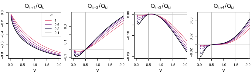
Figure 1: For dimension $d=1$, $Q_{i,i+h}/Q_{i,i}$ as a function of $\nu$ for various values of $h$ and several inverse range parameters $\alpha$. Vertical lines indicate values set to zero in the SPDE approximation.

Section 2 contains a general background on spectral theory for stationary random fields on grids of points. Section 3 provides a theoretical study of spectral properties of Matérn covariances in particular, and of the SPDE approximation. Section 4 includes numerical and simulation results, and Section 5 concludes with a discussion. The appendix has an extended background and proofs of theorems.

2 Background

The details for all derivations in this section are spelled out in Appendix A. Let $Y:\mathbb{R}^{d}\to\mathbb{R}$ be a stationary process with autocovariance function $A[\,h\,]=\mathrm{Cov}\{Y[\,x+h\,],Y[\,x\,]\}$. Due to Bochner’s theorem (cf. Stein,, 1999), $A[\,\,]$ is positive definite when

$$\int_{\mathbb{R}^{d}}A[\,h\,]e^{-i2\pi\omega\cdot h}dh\coloneqq{A}(\omega)>0\quad\mbox{for all }\omega\in\mathbb{R}^{d}.$$ (2)

We call ${A}()$ the spectral density for $A[\,\,]$. Our notational convention uses the same letter for the spectral density and covariance function, distinguishing the two with the type of bracket: round for spectral densities and square for covariances. For $\Delta>0$, define the interval $\mathbb{T}_{\Delta}=[0,1/\Delta]$ and hypercube $\mathbb{T}_{\Delta}^{d}$. When $h\in\mathbb{Z}^{d}$, the inverse Fourier transform can be rewritten as

$$A[\,\Delta h\,]=\int_{\mathbb{T}_{\Delta}^{d}}\,\,\sum_{k\in\mathbb{Z}^{d}}{A}(\omega+k/\Delta)e^{i2\pi\Delta\omega\cdot h}d\omega\eqqcolon A_{\Delta}[\,h\,],$$ (3)

which uses the aliasing property of complex exponentials and introduces a notation $A_{\Delta}[\,\,]:\mathbb{Z}^{d}\to\mathbb{R}$ for covariances on a grid of points with spacing $\Delta$. We define

$${A}_{\Delta}(\omega)=\sum_{k\in\mathbb{Z}^{d}}{A}(\omega+k/\Delta)$$ (4)

to be the aliased spectral density for $A$ on a grid with spacing $\Delta$. The discrete covariances and the aliased spectral density are related via

$$A_{\Delta}[\,h\,]=\int_{\mathbb{T}_{\Delta}^{d}}A_{\Delta}(\omega)e^{i2\pi\Delta\omega\cdot h}d\omega,\quad A_{\Delta}(\omega)=\Delta^{d}\sum_{h\in\mathbb{Z}^{d}}A_{\Delta}[\,h\,]e^{-i2\pi\Delta\omega\cdot h},$$ (5)

so that $A_{\Delta}[\,\,]$ is the integral Fourier transform of $A_{\Delta}()$ over $\mathbb{T}_{\Delta}^{d}$, and $A_{\Delta}()$ is the infinite discrete Fourier transform of $A_{\Delta}[\,\,]$. We say that $A_{\Delta}^{-1}[\,\,]$ is the inverse of $A_{\Delta}[\,\,]$ if

$$\Delta^{d}\sum_{k\in\mathbb{Z}^{d}}A_{\Delta}[\,h-k\,]A_{\Delta}^{-1}[\,k\,]=\mathbbm{1}[\,h\,].$$ (6)

where $\mathbbm{1}[\,h\,]=1$ when $h=0$ and $0$ otherwise. We call $A_{\Delta}^{-1}[\,\,]$ the inverse operator. Taking the infinite discrete Fourier transform of both sides of (6) reveals that

$$A_{\Delta}(\omega)A^{-1}_{\Delta}(\omega)=\Delta^{d},$$ (7)

meaning that the spectrum of $A_{\Delta}^{-1}$ is the $\Delta^{d}$ times the reciprocal of the spectrum of $A_{\Delta}$.

We can also define the square root of $A_{\Delta}$ to be the operator $A^{1/2}_{\Delta}$ for which

$$A_{\Delta}[\,h\,]=\Delta^{d}\sum_{k\in\mathbb{Z}^{d}}A^{1/2}_{\Delta}[\,h-k\,]A^{1/2}_{\Delta}[\,-k\,]$$ (8)

Note the difference between (6), which is meant to mimic the matrix multiplication $BB^{-1}$, and (8), which is meant to mimic the matrix multiplication $BB^{T}$. Taking the Fourier transform of both sides reveals that

$$A_{\Delta}^{1/2}(\omega)A_{\Delta}^{1/2}(\omega)^{*}=A_{\Delta}(\omega),$$ (9)

where $*$ denotes complex conjugate. The spectral density of $A_{\Delta}^{1/2}$ is the complex square root of the spectral density of $A_{\Delta}$. This means that the square root spectral density is unique only up to multiplication by $\exp(i2\pi\omega x)$. This is a necessary consequence of the translation-invariance property of stationary processes, since multiplication by $\exp(i2\pi\omega x)$ in the spectral domain corresponds to translation by $x$ in the natural domain. Square root operators may also have inverses; their spectral densities again follow the reciprocal relationship.

Square root operators are useful for the simulation of processes that have particular covariances. Let $W:\mathbb{Z}^{d}\to\mathbb{R}$ be a white noise process defined on a the integer lattice, that is, its autocovariance function is the identity function $\mathbbm{1}[\,h\,]$. Define $Y:(\Delta\mathbb{Z})^{d}\to\mathbb{R}$ as

$$Y[\,\Delta j\,]=\Delta^{d/2}\sum_{k\in\mathbb{Z}^{d}}A_{\Delta}^{1/2}[\,j-k\,]W[\,k\,].$$ (10)

The covariance function for $Y$ is $A_{\Delta}$. The representation in (10) is exploited in the convolution method of Higdon, (1998). The inverse of the square root operator can be used to decorrelate a process. For a process $Y$ on $(\Delta\mathbb{Z})^{d}$ with autocovariance function $A_{\Delta}$, let $A_{\Delta}^{-1/2}$ be the square root operator for $A_{\Delta}^{-1}$, and define $W$ on $\mathbb{Z}^{d}$ as

$$W[\,j\,]=\Delta^{d/2}\sum_{k\in\mathbb{Z}^{d}}A_{\Delta}^{-1/2}[\,k-j\,]Y[\,\Delta k\,].$$ (11)

The process $W$ has covariance function $\mathbbm{1}[\,h\,]$ and is thus a white noise process.

3 Matérn Covariances and SPDE Approximations

The stationary Matérn covariance function is

$$M[\,h\,;\,\nu,d\,]=\frac{\sigma^{2}(\alpha\|h\|)^{\nu}K_{\nu}(\alpha\|h\|)}{\Gamma(\nu)2^{\nu-1}}=\int_{\mathbb{R}^{d}}\frac{\sigma^{2}N_{\alpha,\nu,d}}{\big{(}\alpha^{2}+4\pi^{2}\|\omega\|^{2}\big{)}^{\nu+d/2}}e^{i2\pi\omega\cdot h}d\omega,$$ (12)

where $N_{\alpha,\nu,d}=2^{d}\pi^{d/2}\alpha^{2\nu}\Gamma(\nu+d/2)/\Gamma(\nu)$ is a normalizing constant (Williams and Rasmussen,, 2006). The aliased spectral density is

$${M}_{\Delta}(\omega\,;\,\nu,d)=\sum_{k\in\mathbb{Z}^{d}}\sigma^{2}N_{\alpha,\nu,d}\big{(}\alpha^{2}+4\pi^{2}\|\omega+k/\Delta\|^{2}\big{)}^{-\nu-d/2}.$$ (13)

3.1 One Dimension, $\nu=1/2$

From here on, we set $\sigma^{2}=1$ to simplify the expressions. When $d=1$ and $\nu=1/2$, the aliased spectral density has the closed form

$$M_{\Delta}(\omega\,;\,1/2,1)=\Delta\frac{1-e^{-2\Delta\alpha}}{1+e^{-2\Delta\alpha}-e^{-\Delta\alpha}e^{-i\omega 2\pi\Delta}-e^{-\Delta\alpha}e^{+i\omega 2\pi\Delta}},$$ (14)

which can be proven by taking the discrete Fourier transform of the covariance function. The inverse spectral density is $\Delta$ times the reciprocal,

$$M^{-1}_{\Delta}(\omega\,;\,1/2,1)=\frac{1+e^{-2\Delta\alpha}-e^{-\Delta\alpha}e^{-i\omega 2\pi\Delta}-e^{-\Delta\alpha}e^{+i\omega 2\pi\Delta}}{1-e^{-2\Delta\alpha}},$$ (15)

and thus the inverse operator is

$$M^{-1}_{\Delta}[\,h\,;\,1/2,1\,]=\left\{\begin{array}[]{ll}(1+e^{-2\Delta\alpha})/(1-e^{-2\Delta\alpha})&h=0\\ -e^{-\Delta\alpha}/(1-e^{-2\Delta\alpha})&|h|=1\\ 0&|h|>1.\end{array}\right.$$ (19)

The SPDE approximation for the inverse operator in Lindgren et al., (2011) is

$$\widetilde{M}_{\Delta}^{-1}[\,h\,;\,1/2,1\,]=\left\{\begin{array}[]{ll}\frac{\alpha\Delta}{2}+\frac{1}{\alpha\Delta}&\hskip 3.69885pth\hskip 2.84526pt=0\\ -\frac{1}{2\alpha\Delta}&|h|=1\\ 0&|h|>1.\end{array}\right.$$ (23)

which corresponds to spectral density

$$\widetilde{M}_{\Delta}(\omega\,;\,1/2,1)=\Delta\Big{(}\frac{\alpha\Delta}{2}+\frac{1}{\alpha\Delta}-\frac{1}{2\alpha\Delta}e^{-i\omega 2\pi\Delta}-\frac{1}{2\alpha\Delta}e^{+i\omega 2\pi\Delta}\Big{)}^{-1}.$$ (24)

Our first theorem establishes that the true and SPDE spectral densities for $d=1,\nu=1/2$ converge to the same values at frequencies $0$ and $1/(2\Delta)$ for small $\alpha\Delta$.

Theorem 1.

$$\frac{M_{\Delta}(0\,;\,1/2,1)}{2/\alpha} =1+O(\alpha^{2}\Delta^{2}) \frac{M_{\Delta}\big{(}\frac{1}{2\Delta}\,;\,1/2,1\big{)}}{2/\alpha} =\frac{\alpha^{2}\Delta^{2}}{4}+O(\alpha^{4}\Delta^{4})$$

$$\frac{\widetilde{M}_{\Delta}(0\,;\,1/2,1)}{2/\alpha} =1 \frac{\widetilde{M}_{\Delta}\big{(}\frac{1}{2\Delta}\,;\,1/2,1\big{)}}{2/\alpha} =\frac{\alpha^{2}\Delta^{2}}{4}+O(\alpha^{4}\Delta^{4}).$$

Proofs for all theoretical results are in Appendix B. Thorem 1 provides evidence that the SPDE approximation for $\nu=1/2$, $d=1$ is a good approximation to the true model when $\alpha\Delta$ is small; their spectral densities are similar at the lowest frequency ($\omega=0$) when the power is greatest and at the highest frequency ($\omega=\Delta^{-1}/2$) when the power is smallest, implying that the both the SPDE spectral density and its reciprocal may be good approximations to the truth, which in turn implies that both the covariance operator and its inverse may be good approximations.

3.2 One Dimension, $\nu=3/2$

When $\nu=3/2$, the aliased spectral density is

$${M}_{\Delta}(\omega\,;\,3/2,1) =\sum_{k\in\mathbb{Z}}\frac{4\alpha^{3}}{[\alpha^{2}+4\pi^{2}(\omega+k/\Delta)^{2}]^{2}}.$$ (25)

The SPDE approximation in Lindgren et al., (2011) to the inverse operator is simply the convolution of the $\nu=1/2$ approximation (23) with itself (here, normalizing constants are chosen so that $M_{\Delta}(0\,;\,3/2,1)\to\widetilde{M}_{\Delta}(0\,;\,3/2,1)=4/\alpha$ as $\alpha\Delta\to 0$),

$$(\alpha\Delta)\widetilde{M}_{\Delta}^{-1}[\,h\,;\,3/2,1\,]=\left\{\begin{array}[]{ll}\Big{(}\frac{\alpha\Delta}{2}+\frac{1}{\alpha\Delta}\Big{)}^{2}+\frac{1}{2\alpha^{2}\Delta^{2}}&\hskip 3.69885pth\hskip 2.84526pt=0\\ -\frac{1}{2}-\frac{1}{\alpha^{2}\Delta^{2}}&|h|=1\\ \frac{1}{4\alpha^{2}\Delta^{2}}&|h|=2\\ 0&|h|>2,\end{array}\right.$$ (30)

which means that the spectral density for the $\nu=3/2$ SPDE inverse operator is simply the square of spectral density for the $\nu=1/2$ SPDE inverse operator (24),

$$\widetilde{M}_{\Delta}^{-1}(\omega\,;\,3/2,1)=\frac{1}{\alpha\Delta}\Big{(}\frac{\alpha\Delta}{2}+\frac{1}{\alpha\Delta}-\frac{1}{2\alpha\Delta}e^{-i\omega 2\pi\Delta}-\frac{1}{2\alpha\Delta}e^{+i\omega 2\pi\Delta}\Big{)}^{2},$$ (31)

and the spectral density for the $\nu=3/2$ SPDE covariance operator is

$$\widetilde{M}_{\Delta}(\omega\,;\,3/2,1)=\alpha\Delta^{2}\Big{(}\frac{\alpha\Delta}{2}+\frac{1}{\alpha\Delta}-\frac{1}{2\alpha\Delta}e^{-i\omega 2\pi\Delta}-\frac{1}{2\alpha\Delta}e^{+i\omega 2\pi\Delta}\Big{)}^{-2}.$$ (32)

Note however, that the aliased Matérn spectral density for $\nu=3/2$ in (25) is not simply the square of the aliased $\nu=1/2$ spectral density in (14); rather, we alias the square of the unaliased $\nu=1/2$ spectral density. The SPDE appproximation reverses the order of operations, squaring the aliased spectral density. This subtle difference leads to the SPDE approximation assigning too much power at the highest frequencies, made explicit in the following theorem:

Theorem 2.

$$\frac{M_{\Delta}(0\,;\,3/2,1)}{4/\alpha} =1+O(\alpha^{4}\Delta^{4}) \frac{M_{\Delta}\big{(}\frac{1}{2\Delta}\,;\,3/2,1\big{)}}{4/\alpha} =\frac{\alpha^{4}\Delta^{4}}{48}+O(\alpha^{6}\Delta^{6})$$

$$\frac{\widetilde{M}_{\Delta}(0\,;\,3/2,1)}{4/\alpha} =1 \frac{\widetilde{M}_{\Delta}\big{(}\frac{1}{2\Delta}\,;\,3/2,1\big{)}}{4/\alpha} =\frac{\alpha^{4}\Delta^{4}}{16}+O(\alpha^{6}\Delta^{6}).$$

When scaled by $4/\alpha$, both spectral densities converge to 1 when $\omega=0$ and $\alpha\Delta\to 0$, but they converge to two different values, $\alpha^{4}\Delta^{4}/48$ and $\alpha^{4}\Delta^{4}/16$, when $\omega=\Delta^{-1}/2$, meaning that the SPDE spectral density assigns three times too much power at the highest frequency. The inaccuracy of the spectral density at high frequencies impacts the quality of the approximation to the reciprocal of the spectral density, seen in Figure 2, and to the inverse operator, as evidenced in Figure 1.

Figure 2: For $d=1$, $\nu=3/2$, $\alpha=0.4$, true aliased spectral density and its reciprocal (lines) and SPDE approximation to the aliased spectral density and its reciprocal (circles).

3.3 Two Dimensions

The aliased spectral density for the Matérn in two dimensions is

$$M_{\Delta}(\omega\,;\,\nu,2)=4\pi\alpha^{2}\sum_{k\in\mathbb{Z}^{2}}\big{[}\alpha^{2}+4\pi^{2}(\omega_{1}+k_{1}/\Delta)^{2}+4\pi^{2}(\omega_{2}+k_{2}/\Delta)^{2}\big{]}^{-\nu-1}.$$ (33)

The following theorem establishes properties of the aliased Matérn spectral density for $\nu=1$ at the lowest frequency and at high frequencies in one and both spatial dimensions.

Theorem 3.

$$\frac{M_{\Delta}((0,0)\,;\,1,2)}{4\pi/\alpha^{2}} =1+\frac{\alpha^{4}\Delta^{4}}{258.6}+O(\alpha^{6}\Delta^{6})$$ (34)

$$\frac{M_{\Delta}\big{(}(\frac{1}{2\Delta},0)\,;\,1,2\big{)}}{4\pi/\alpha^{2}} =\frac{\alpha^{4}\Delta^{4}}{43.10}+O(\alpha^{6}\Delta^{6})$$ (35)

$$\frac{M_{\Delta}\big{(}(\frac{1}{2\Delta},\frac{1}{2\Delta})\,;\,1,2\big{)}}{4\pi/\alpha^{2}} =\frac{\alpha^{4}\Delta^{4}}{86.20}+O(\alpha^{6}\Delta^{6})$$ (36)

The numbers 258.6, 43.10, and 86.20 are the result of numerical calculations and are rounded to one or two decimals. They are available to higher accuracy. Details are given in the proof in the supplementary material. The SPDE approximation to the inverse operator is

$$4\pi(\alpha\Delta)^{2}\widetilde{M}_{\Delta}^{-1}[\,h\,;\,1,2\,]=\left\{\begin{array}[]{rl}(4+\alpha^{2}\Delta^{2})^{2}+4&\quad h=(0,0)\\ -2(4+\alpha^{2}\Delta^{2})&\quad h=(0,1),(0,-1),(1,0),(-1,0)\\ 2&\quad h=(1,1),(1,-1),(-1,1),(-1,-1)\\ 1&\quad h=(2,0),(0,2),(-2,0),(0,-2)\\ 0&\quad\mbox{otherwise},\end{array}\right.$$ (42)

which corresponds to the spectral density

$$\widetilde{M}_{\Delta}(\omega\,;\,1,2)=4\pi\alpha^{2}\Delta^{4}\Big{(}4+\alpha^{2}\Delta^{2}-e^{i2\pi\Delta\omega_{1}}-e^{-i2\pi\Delta\omega_{1}}-e^{i2\pi\Delta\omega_{2}}-e^{-i2\pi\Delta\omega_{2}}\Big{)}^{-2}.$$ (43)

The normalizing constants are chosen so that $M_{\Delta}((0,0)\,;\,1,2)\to\widetilde{M}_{\Delta}((0,0)\,;\,1,2)=4\pi/\alpha^{2}$ as $\alpha\Delta\to 0$. The following theorem establishes the behavior of $\widetilde{M}_{\Delta}(\omega\,;\,1,2)$ at the same frequencies in Theorem 3.

Theorem 4.

$$\frac{\widetilde{M}_{\Delta}((0,0)\,;\,1,2)}{4\pi/\alpha^{2}} =1$$ (44)

$$\frac{\widetilde{M}_{\Delta}\big{(}(\frac{1}{2\Delta},0)\,;\,1,2\big{)}}{4\pi/\alpha^{2}} =\frac{\alpha^{4}\Delta^{4}}{16}+O(\alpha^{6}\Delta^{6})$$ (45)

$$\frac{\widetilde{M}_{\Delta}\big{(}(\frac{1}{2\Delta},\frac{1}{2\Delta})\,;\,1,2\big{)}}{4\pi/\alpha^{2}} =\frac{\alpha^{4}\Delta^{4}}{64}+O(\alpha^{6}\Delta^{6})$$ (46)

Theorems 3 and 4 imply that when $\alpha\Delta$ is small, the SPDE approach over-approximates the spectral density by a factor of $43.1/16=2.69$ at $\omega=(\Delta^{-1}/2,0)$ and $86.2/64=1.35$ at $\omega=(\Delta^{-1}/2,\Delta^{-1}/2)$. Figure 3 contains an example where the ratio between the SPDE spectral density and the true spectral density varies between 0.999 at $\omega=(0,0)$, 2.680 at $\omega=(\Delta^{-1}/2,0)$ and 1.345 at $\omega=(\Delta^{-1}/2,\Delta^{-1}/2)$.

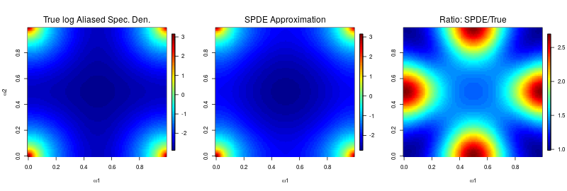
Figure 3: True spectral density for $\nu=1$, $\alpha=0.5$, SPDE approximation to the spectral density, and the ratio of the two. The ratio is near 1.00 at $(0,0)$, near 2.69 at $(1/2\Delta,0)$ and near 1.35 at $(1/2\Delta,1/2\Delta)$, as predicted by the theory.

4 Numerical and Simulation Results

4.1 Dependence of Inverse Operator on Smoothness

In Figures 4 and 5, we plot $M^{-1}_{\Delta}[\,0\,;\,\nu,d\,]$ and $M^{-1}_{\Delta}[\,h\,;\,\nu,d\,]/M^{-1}_{\Delta}[\,0\,;\,\nu,d\,]$ for $\Delta=1$, $d=1,2$, and for a range of values of smoothness parameter $\nu$ and inverse range $\alpha$. First consider $d=1$. When $h=1$, the operator is always negative. When $h=2$, the operator is exactly 0 for $\nu=0.5$, agreeing with the theory from Section 3 of the main document, which says that the operator is exactly zero when $\nu=0.5$ for all $|h|>1$. When $h=3$, there is an additional zero near $\nu=0.7$ but there is no zero at $\nu=1.5$; the SPDE approximation (Lindgren et al.,, 2011) sets the operator equal to zero when $\nu=1.5$ for all $|h|>2$. When $h=4$, the only zero is at $\nu=0.5$. For $d=2$, the SPDE approximation sets the inverse operator to zero when $\nu=1.0$ and $|h_{1}|+|h_{2}|>2$. Figure 5 shows that while there are some zeros in the inverse operator, they generally do not appear at or near $\nu=1.0$. For example, when $h=(1,2)$, the inverse operator is nearly at its maximum when $\nu=1.0$. While the magnitudes of the operators generally decrease as $\|h\|$ increases, there does not appear to be anything particularly sparse about the cases $d=1,\nu=3/2$ or $d=2,\nu=1$.

4.2 Simulation Study

We simulated two-dimensional data on a $(30,30)$ grid under a Matérn model with $\sigma^{2}=2$, $\alpha=0.2$, and $\nu=1$, and with three noise levels, $\tau^{2}=0$, $\tau^{2}=0.01$, and $\tau^{2}=0.1$. The model is parameterized so that the total variance is $\sigma^{2}(1+\tau^{2})$, which means that $1/\tau^{2}$ is the signal to noise ratio. Data are simulated using a standard method of forming the $900\times 900$ true covariance matrix and multiplying its Cholesky factor by a vector of standard normals. We assumed that the mean was known to be zero, and the smoothness parameter $\nu$ was known to be 1. In the zero noise case ($\tau^{2}=0$), we assumed that the noise parameter was known to be zero; otherwise, we estimated the noise parameter $\tau^{2}$ along with $\sigma^{2}$ and $\alpha$.

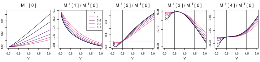
Figure 4: For dimension $d=1$, $M_{1}^{-1}[\,h\,;\,\nu,1\,]/M_{1}^{-1}[\,0\,;\,\nu,1\,]$ as a function of $\nu$ for various values of $h$ and several inverse range parameters $\alpha$. Vertical lines indicate values set to zero in the SPDE approximation.

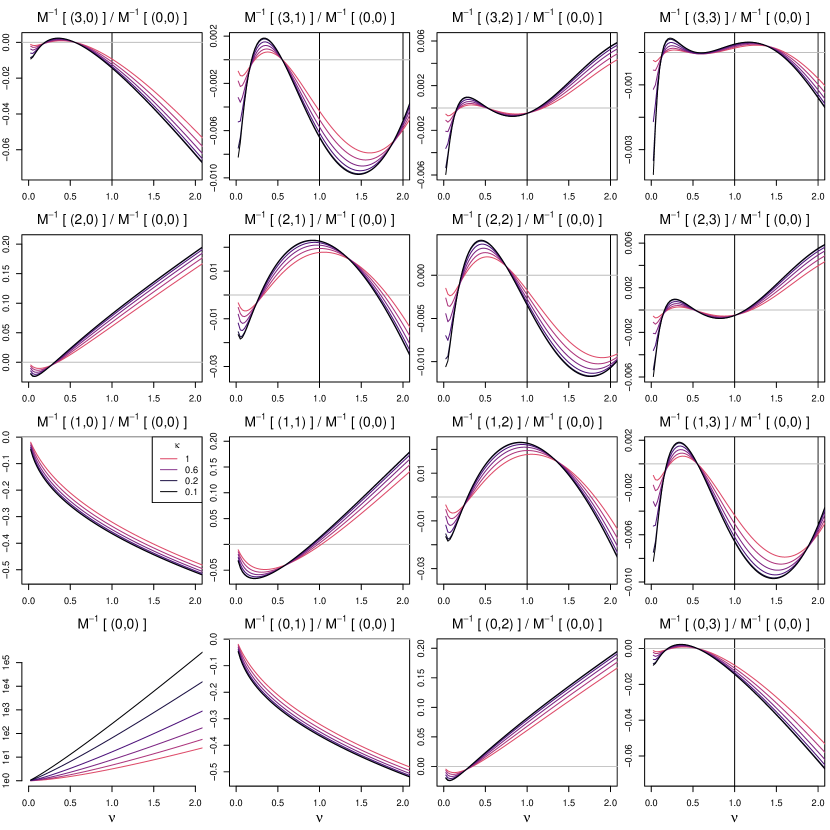
Figure 5: For dimension $d=2$, $M_{1}^{-1}[\,h\,;\,\nu,2\,]/M_{1}^{-1}[\,0\,;\,\nu,2\,]$ as a function of $\nu$ for various values of $h$ and several inverse range parameters $\alpha$. Vertical lines indicate values set to zero in the SPDE approximation.

Parameters were estimated via maximum likelihood under each of the following scenarios:

1. true model

2. Vecchia’s approximation using GpGp R package.

3. SPDE approximation

4. SPDE approximation double resolution

For the SPDE methods, we ameliorate edge effects by using the approximations to compute covariances under periodic boundary conditions on a $(100,100)$ grid and extract the covariances from a $(30,30)$ subgrid. Whereas the data grid has $\Delta=1$, the SPDE double resolution method computes covariances using $\Delta=1/2$, leading to different covariances than those obtained by the SPDE approximation with $\Delta=1$. Vecchia’s approximation (Vecchia,, 1988) is implemented in the GpGp R package (Guinness and Katzfuss,, 2020). GpGp estimates a constant mean parameter and has minor penalties on small nuggets; see Guinness, (2019) for details.

Figure 6 contains results of the simulation study over 500 simulation replicates. Each black point in the plot is an estimate of the microergodic parameter (Zhang,, 2004) $\widehat{\sigma}^{2}\widehat{\alpha}^{2}$. The estimates are sorted and evenly spaced in the horizontal direction, creating a visualization of the empirical quantile function of the estimates. We include a magenta line for the true value $2(0.2)^{2}=0.08$. Several interesting things arise from the simulation study. Focusing on the zero noise case first, the SPDE approximations underestimate the microergodic parameter. This corresponds to an overestimation of the spatial range since $\alpha$ is an inverse range parameter. This makes sense given that the SPDE approximation assigns too much power at the highest frequencies; the likelihood must select a larger range parameter to dampen the power. The estimates improve somewhat in SPDE Double Resolution but still have a bias. When noise is added, the SPDE approximations begin to improve. Vecchia’s approximation is accurate in every case.

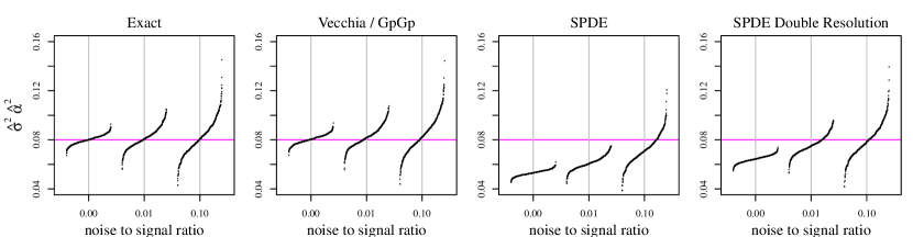
Figure 6: Estimates of $\widehat{\sigma}^{2}\widehat{\alpha}^{2}$, over 500 simulation replicates of data on grid of size $(30,30)$ for three noise levels. Each black point is a parameter estimate. Estimates are sorted and spaced evenly in the horizontal direction to create visualization of empirical quantile function. True value $\sigma^{2}\alpha^{2}=2(0.2)^{2}=0.08$ indicated in magenta.

5 Discussion

The SPDE approximation has proven to be useful as a computational tool and as a conceptual tool for defining extensions to irregularly-spaced data, models on manifolds, and to non-stationary models (Fuglstad et al.,, 2015; Bakka et al.,, 2018). This paper does not question the usefulness of the SPDE approach as a tool for data analysis. Rather, it is a study of the ability of the SPDE approach to approximate Matérn models on grids.

We study SPDE approximations to Matérn fields observed at point locations on a grid, as opposed to observations of gridbox averages. While SPDE approximations have been applied in both cases, the spectral properties of gridbox average fields are different, and it is not clear to the author whether the SPDE approximations would be more or less accurate in the gridbox average case. This is certainly and interesting question worthy of future study. In addition, it would be interesting to explore extensions to irregularly sampled locations. In both of these cases, a study of the impact of the approximations on predictions is also warranted. It seems plausible that if the approximate model is used for both inferring parameters and generating predictions, the resulting predictions would be reasonably accurate.

Acknowledgements

This work was supported by the National Science Foundation under grant No. 1916208 and the National Institutes of Health under grant No. R01ES027892. The author is grateful to have received helpful feedback on an early draft from Matthias Katzfuss, Michael Stein, and Ethan Anderes, and from an Associate Editor and two anonymous reviewers, one of which pointed out an mistake in the first version.

Appendix A Extended Background

The first proposition establishes the aliasing property of complex exponential and uses it to express the covariances as an integral on a bounded domain instead of an infinite domain. Note that we define $\mathbb{T}_{\Delta}=[0,\Delta^{-1}]$ as opposed to $[-\Delta^{-1}/2,\Delta^{-1}/2]$, which is perhaps a more common convention. Both lead to equivalent integrals, as all of the aliased functions are periodic on $\mathbb{T}_{\Delta}$. We prefer this convention because it more closely maps onto how most software organizes their fast Fourier transform functions. For example, in R, the ‘fft’ function returns a vector whose first entry corresponds to frequency $0$ instead of frequency $-\Delta^{-1}/2$.

Proposition 1.

(Aliasing) For $h\in\mathbb{Z}^{d}$,

$$A[\,\Delta h\,]=\int_{\mathbb{T}_{\Delta}^{d}}\Big{[}\sum_{k\in\mathbb{Z}^{d}}{A}(\omega+k/\Delta)\Big{]}\exp({i2\pi\Delta\omega\cdot h})d\omega$$ (47)

Proof.

Using Bochner’s theorem and splitting the integral into domains of size $\mathbb{T}_{\Delta}^{d}$,

$$A[\,\Delta h\,]=\sum_{k\in\mathbb{Z}^{d}}\int_{\mathbb{T}^{d}_{\Delta}}A(\omega+k/\Delta)\exp(i2\pi(\omega+k/\Delta)\cdot\Delta h)d\omega.$$ (48)

Exchanging sum with integral gives

$$A[\,\Delta h\,]=\int_{\mathbb{T}^{d}_{\Delta}}\sum_{k\in\mathbb{Z}^{d}}A(\omega+k/\Delta)\exp(i2\pi(\omega+k/\Delta)\cdot\Delta h)d\omega.$$ (49)

The complex exponential can be expanded as

$$\exp(i2\pi(\omega+k/\Delta)\cdot\Delta h)=\exp(i2\pi\Delta\omega\cdot h+i2\pi k\cdot h)=\exp(i2\pi\Delta\omega\cdot h)\exp(i2\pi k\cdot h).$$ (50)

Since $k\in\mathbb{Z}^{2}$ and $h\in\mathbb{Z}^{2}$, $k\cdot h=n$ is an integer, and thus the complex exponential is

$$\exp(i2\pi\Delta\omega\cdot h)\exp(i2\pi n)=\exp(i2\pi\Delta\omega\cdot h).$$ (51)

Plugging this expression back into the integral gives

$$A[\,\Delta h\,]=\int_{\mathbb{T}^{d}_{\Delta}}\Big{[}\sum_{k\in\mathbb{Z}^{d}}A(\omega+k/\Delta)\Big{]}\exp(i2\pi\Delta\omega\cdot h)d\omega,$$ (52)

as desired. ∎

The second proposition establishes the reciprocal relationship between the spectral density of the covariance operator and the spectral density of the inverse operator.

Proposition 2.

(Reciprocal Relationship of Inverse) For all $\omega\in\mathbb{T}_{\Delta}^{d}$,

$$A_{\Delta}(\omega)A_{\Delta}^{-1}(\omega)=\Delta^{d}.$$ (53)

Proof.

By definition, the inverse satisfies

$$\Delta^{d}\sum_{k\in\mathbb{Z}^{d}}A_{\Delta}[\,h-k\,]A_{\Delta}^{-1}[\,k\,]=\mathbbm{1}[\,h\,].$$ (54)

Take the infinite DFT of both sides,

$$\Delta^{2d}\sum_{h\in\mathbb{Z}^{d}}\sum_{k\in\mathbb{Z}^{d}}A_{\Delta}[\,h-k\,]A_{\Delta}^{-1}[\,k\,]e^{-i2\pi\Delta\omega\cdot h} =\Delta^{d}\sum_{h\in\mathbb{Z}^{d}}\mathbbm{1}[\,h\,]e^{-i2\pi\Delta\omega\cdot h}$$ (55)

$$\Delta^{d}\sum_{k\in\mathbb{Z}^{d}}A_{\Delta}^{-1}[\,k\,]e^{-i2\pi\Delta\omega\cdot k}\Delta^{d}\sum_{h\in\mathbb{Z}^{d}}A_{\Delta}[\,h-k\,]e^{-i2\pi\Delta\omega\cdot(h-k)} =\Delta^{d}$$ (56)

$$A_{\Delta}^{-1}(\omega)A_{\Delta}(\omega) =\Delta^{d}.$$ (57)

∎

Proposition 3.

(Square Root spectral density) For all $\omega\in\mathbb{T}_{\Delta}^{d}$,

$$A_{\Delta}^{1/2}(\omega)A_{\Delta}^{1/2}(\omega)^{*}=A_{\Delta}(\omega).$$ (58)

Proof.

By definition, the square root operator satisfies

$$\Delta^{d}\sum_{k\in\mathbb{Z}^{d}}A_{\Delta}^{1/2}[\,h-k\,]A_{\Delta}^{1/2}[\,-k\,]=A_{\Delta}[\,h\,].$$ (59)

Taking the infinite DFT of both sides,

$$\Delta^{2d}\sum_{h\in\mathbb{Z}^{d}}\sum_{k\in\mathbb{Z}^{d}}A_{\Delta}^{1/2}[\,h-k\,]A_{\Delta}^{1/2}[\,-k\,]e^{-i2\pi\Delta\omega\cdot h} =\Delta^{d}\sum_{h\in\mathbb{Z}^{d}}A_{\Delta}[\,h\,]e^{-i2\pi\Delta\omega\cdot h}$$ (60)

$$\Delta^{d}\sum_{k\in\mathbb{Z}^{d}}A_{\Delta}^{1/2}[\,-k\,]e^{-i2\pi\Delta\omega\cdot k}\Delta^{d}\sum_{h\in\mathbb{Z}^{d}}A_{\Delta}^{1/2}[\,h-k\,]e^{-i2\pi\Delta\omega\cdot(h-k)} =A_{\Delta}(\omega)$$ (61)

$$A_{\Delta}^{1/2}(\omega)^{*}A_{\Delta}^{1/2}(\omega) =A_{\Delta}(\omega).$$ (62)

∎

Proposition 4.

(Convolution Method of Simulation) If the mean-zero process $W:\mathbb{Z}^{d}\to\mathbb{R}$ has covariance operator $\mathbbm{1}[\,h\,]$, and

$$Y[\,\Delta h\,]=\Delta^{d/2}\sum_{k\in\mathbb{Z}^{d}}A_{\Delta}^{1/2}[\,h-k\,]W[\,k\,],$$ (63)

then $\mathrm{Cov}(Y[\,\Delta(h)\,],Y[\,\Delta j\,])=A_{\Delta}[\,h-j\,]$.

Proof.

$$\mathrm{Cov}(Y[\,\Delta h\,],Y[\,\Delta j\,]) =E\Big{[}\Delta^{d/2}\sum_{k\in\mathbb{Z}^{d}}A_{\Delta}^{1/2}[\,h-k\,]W[\,k\,]\Delta^{d/2}\sum_{m\in\mathbb{Z}^{d}}A_{\Delta}^{1/2}[\,j-m\,]W[\,m\,]\Big{]}$$ (64)

$$=\Delta^{d}\sum_{k\in\mathbb{Z}^{d}}A_{\Delta}^{1/2}[\,h-k\,]A_{\Delta}^{1/2}[\,j-k\,]$$ (65)

$$=\Delta^{d}\sum_{\ell\in\mathbb{Z}^{d}}A_{\Delta}^{1/2}[\,h-j-\ell\,]A_{\Delta}^{1/2}[\,-\ell\,]$$ (66)

$$=A_{\Delta}[\,h-j\,].$$ (67)

∎

Proposition 5.

If the mean-zero process $Y:(\Delta\mathbb{Z})^{d}\to\mathbb{R}$ has covariance operator $A_{\Delta}$, and

$$W[\,h\,]=\Delta^{d/2}\sum_{k\in\mathbb{Z}^{d}}A_{\Delta}^{-1/2}[\,h-k\,]Y[\,\Delta k\,],$$ (68)

then $\mathrm{Cov}(W[\,h\,],W[\,j\,])=\mathbbm{1}[\,h-j\,]$.

Proof.

$$\mathrm{Cov}( W[\,h\,],W[\,j\,])$$ (69)

$$=E\Big{[}\Delta^{d/2}\sum_{k\in\mathbb{Z}^{d}}A_{\Delta}^{-1/2}[\,h-k\,]Y[\,\Delta k\,]\Delta^{d/2}\sum_{m\in\mathbb{Z}^{d}}A_{\Delta}^{-1/2}[\,j-m\,]Y[\,\Delta m\,]\Big{]}$$ (70)

$$=\Delta^{d}\sum_{k\in\mathbb{Z}^{d}}\sum_{m\in\mathbb{Z}^{d}}A_{\Delta}^{-1/2}[\,h-k\,]A_{\Delta}^{-1/2}[\,j-m\,]A_{\Delta}[\,m-k\,]$$ (71)

$$=\Delta^{d}\sum_{k\in\mathbb{Z}^{d}}\sum_{m\in\mathbb{Z}^{d}}A_{\Delta}^{-1/2}[\,h-k\,]A_{\Delta}^{-1/2}[\,j-m\,]\Delta^{d}\sum_{\ell\in\mathbb{Z}^{d}}A_{\Delta}^{1/2}[\,m-k-\ell\,]A_{\Delta}^{1/2}[\,-\ell\,]$$ (72)

$$=\Delta^{d}\sum_{k\in\mathbb{Z}^{d}}\sum_{\ell\in\mathbb{Z}^{d}}A_{\Delta}^{-1/2}[\,h-k\,]A_{\Delta}^{1/2}[\,-\ell\,]\Delta^{d}\sum_{m\in\mathbb{Z}^{d}}A_{\Delta}^{1/2}[\,m-k-\ell\,]A_{\Delta}^{-1/2}[\,j-m\,]$$ (73)

$$=\Delta^{d}\sum_{k\in\mathbb{Z}^{d}}\sum_{\ell\in\mathbb{Z}^{d}}A_{\Delta}^{-1/2}[\,h-k\,]A_{\Delta}^{1/2}[\,-\ell\,]\Delta^{d}\sum_{n\in\mathbb{Z}^{d}}A_{\Delta}^{1/2}[\,j-k-\ell-n\,]A_{\Delta}^{-1/2}[\,n\,]$$ (74)

$$=\Delta^{d}\sum_{k\in\mathbb{Z}^{d}}\sum_{\ell\in\mathbb{Z}^{d}}A_{\Delta}^{-1/2}[\,h-k\,]A_{\Delta}^{1/2}[\,-\ell\,]\mathbbm{1}[\,j-k-\ell\,]$$ (75)

$$=\Delta^{d}\sum_{k\in\mathbb{Z}^{d}}A_{\Delta}^{-1/2}[\,h-k\,]A_{\Delta}^{1/2}[\,k-j\,]$$ (76)

$$=\mathbbm{1}[\,h-j\,]$$ (77)

∎

Appendix B Proofs for Matérn Model

This section contains proofs of Theorems 1-4 from the main document. Theorems 1-3 have precise coefficients on higher-order terms that were omitted from the main document to conserve space. We first state a lemma that is a consequence of Taylor’s Theorem:

Lemma 1.

For $x>0$,

$$(1+x)^{-1} =1-x+x^{2}c(x),\quad 0<c(x)<1$$

$$(1+x)^{-2} =1-2x+x^{2}d(x),\quad 0<d(x)<3$$

Proof.

By Taylor’s Theorem, $(1+x)^{-1}=1-x+x^{2}(1+a(x))^{-3}$, where $0<a(x)<x$. Therefore, $(1+x)^{-1}=1-x+x^{2}c(x),\mbox{where}\quad 0<c(x)<1$. Similarly, $(1+x)^{-2}=1-2x+3x^{2}(1+b(x))^{-4}$, where $0<b(x)<x$. Therefore, $(1+x)^{-2}=1-2x+x^{2}d(x),\mbox{where}\quad 0<d(x)<3$. ∎

Theorem 1.

$$\frac{M_{\Delta}(0\,;\,1/2,1)}{2/\alpha} =1+O(\alpha^{2}\Delta^{2}) \frac{M_{\Delta}\big{(}\frac{1}{2\Delta}\,;\,1/2,1\big{)}}{2/\alpha} =\frac{\alpha^{2}\Delta^{2}}{4}+O(\alpha^{4}\Delta^{4})$$

$$\frac{\widetilde{M}_{\Delta}(0\,;\,1/2,1)}{2/\alpha} =1 \frac{\widetilde{M}_{\Delta}\big{(}\frac{1}{2\Delta}\,;\,1/2,1\big{)}}{2/\alpha} =\frac{\alpha^{2}\Delta^{2}}{4}+O(\alpha^{4}\Delta^{4}).$$

Proof.

We establish each of the four relations in turn. Rearranging terms gives

$$\frac{M_{\Delta}(0:1/2,1)}{2/\alpha}=\alpha^{2}\sum_{k\in\mathbb{Z}}\Big{(}\alpha^{2}+4\pi^{2}k^{2}/\Delta^{2}\Big{)}^{-1}=1+\frac{\alpha^{2}\Delta^{2}}{2\pi^{2}}\sum_{k=1}^{\infty}\frac{1}{k^{2}}\Big{(}1+\frac{\alpha^{2}\Delta^{2}}{4\pi^{2}k^{2}}\Big{)}^{-1}.$$

Applying Lemma 1,

$$\frac{M_{\Delta}(0:1/2,1)}{2/\alpha}=1+\frac{\alpha^{2}\Delta^{2}}{2\pi^{2}}\sum_{k=1}^{\infty}\frac{1}{k^{2}}\Big{(}1-\frac{\alpha^{2}\Delta^{2}}{4\pi^{2}k^{2}}+q_{k}\frac{\alpha^{4}\Delta^{4}}{16\pi^{4}k^{4}}\Big{)},$$

where $0<q_{k}<1$. Evaluating the sums gives

$$\frac{M_{\Delta}(0:1/2,1)}{2/\alpha}=1+\frac{\alpha^{2}\Delta^{2}}{12}-\frac{\alpha^{4}\Delta^{4}}{720}+O(\alpha^{6}\Delta^{6}).$$

The second relation follows directly from plugging $\omega=0$ into the SPDE spectral density. For the third relation, rearranging terms gives

$$\frac{M_{\Delta}(\Delta^{-1}/2:1/2,1)}{2/\alpha} =\alpha^{2}\sum_{k\in\mathbb{Z}}\Big{[}\alpha^{2}+4\pi^{2}\Big{(}\frac{1}{2\Delta}+\frac{k}{\Delta}\Big{)}^{2}\Big{]}^{-1}$$

$$=\frac{2\alpha^{2}\Delta^{2}}{\pi^{2}}\sum_{k=0}^{\infty}\frac{1}{(2k+1)^{2}}\Big{[}1+\frac{\alpha^{2}\Delta^{2}}{\pi^{2}}\frac{1}{(2k+1)^{2}}\Big{]}^{-1}.$$

Applying Lemma 1,

$$\frac{M_{\Delta}(\Delta^{-1}/2:1/2,1)}{2/\alpha}=\frac{2\alpha^{2}\Delta^{2}}{\pi^{2}}\sum_{k=0}^{\infty}\frac{1}{(2k+1)^{2}}\Big{[}1-\frac{\alpha^{2}\Delta^{2}}{\pi^{2}}\frac{1}{(2k+1)^{2}}+p_{k}\frac{\alpha^{4}\Delta^{4}}{\pi^{4}}\frac{1}{(2k+1)^{4}}\Big{]},$$

where $0<p_{k}<1$. Evaluating the sums,

$$\frac{M_{\Delta}(\Delta^{-1}/2:1/2,1)}{2/\alpha}=\frac{\alpha^{2}\Delta^{2}}{4}-\frac{\alpha^{4}\Delta^{4}}{48}+O(\alpha^{6}\Delta^{6}),$$

establishing the third relation. For the fourth relation,

$$\frac{\widetilde{M}(\Delta^{-1}/2:1/2,1)}{2/\alpha}=\frac{\alpha\Delta}{2}\Big{(}\frac{\alpha\Delta}{2}+\frac{2}{\alpha\Delta}\Big{)}^{-1}=\frac{\alpha^{2}\Delta^{2}}{4}\Big{(}1+\frac{\alpha^{2}\Delta^{2}}{4}\Big{)}^{-1}.$$

Applying Lemma 1, for $0<q<1$,

$$\frac{\widetilde{M}(\Delta^{-1}/2:1/2,1)}{2/\alpha}=\frac{\alpha^{2}\Delta^{2}}{4}\Big{(}1-\frac{\alpha^{2}\Delta^{2}}{4}+q\frac{\alpha^{4}\Delta^{4}}{16}\Big{)}=\frac{\alpha^{2}\Delta^{2}}{4}-\frac{\alpha^{4}\Delta^{4}}{16}+O(\alpha^{6}\Delta^{6}).$$

∎

Theorem 2.

$$\frac{M_{\Delta}(0\,;\,3/2,1)}{4/\alpha} =1+O(\alpha^{4}\Delta^{4}) \frac{M_{\Delta}\big{(}\frac{1}{2\Delta}\,;\,3/2,1\big{)}}{4/\alpha} =\frac{\alpha^{4}\Delta^{4}}{48}+O(\alpha^{6}\Delta^{6})$$

$$\frac{\widetilde{M}_{\Delta}(0\,;\,3/2,1)}{4/\alpha} =1 \frac{\widetilde{M}_{\Delta}\big{(}\frac{1}{2\Delta}\,;\,3/2,1\big{)}}{4/\alpha} =\frac{\alpha^{4}\Delta^{4}}{16}+O(\alpha^{6}\Delta^{6}).$$

Proof.

We establish each of the four relations in turn. Rearranging terms gives

$$\frac{M_{\Delta}(0:3/2,1)}{4/\alpha}=\alpha^{4}\sum_{k\in\mathbb{Z}}\Big{(}\alpha^{2}+4\pi^{2}k^{2}/\Delta^{2}\Big{)}^{-2}=1+\frac{\alpha^{4}\Delta^{4}}{8\pi^{4}}\sum_{k=1}^{\infty}\frac{1}{k^{4}}\Big{(}1+\frac{\alpha^{2}\Delta^{2}}{4\pi^{2}k^{2}}\Big{)}^{-2}.$$

Applying Lemma 1,

$$\frac{M_{\Delta}(0:3/2,1)}{4/\alpha}=1+\frac{\alpha^{4}\Delta^{4}}{8\pi^{4}}\sum_{k=1}^{\infty}\frac{1}{k^{4}}\Big{(}1-\frac{\alpha^{2}\Delta^{2}}{2\pi^{2}k^{2}}+\frac{\alpha^{4}\Delta^{4}}{16\pi^{4}k^{4}}q_{k}\Big{)}.$$

where $0<q_{k}<3$. Evaluating the sums gives

$$\frac{M_{\Delta}(0:3/2,1)}{2/\alpha}=1+\frac{\alpha^{4}\Delta^{4}}{720}-\frac{\alpha^{6}\Delta^{6}}{15120}+O(\alpha^{8}\Delta^{8}).$$

The second relation follows directly from plugging $\omega=0$ into the SPDE spectral density. For the third relation, rearranging terms gives

$$\frac{M_{\Delta}(\Delta^{-1}/2:3/2,1)}{4/\alpha} =\alpha^{4}\sum_{k\in\mathbb{Z}}\Big{[}\alpha^{2}+4\pi^{2}\Big{(}\frac{1}{2\Delta}+\frac{k}{\Delta}\Big{)}^{2}\Big{]}^{-2}$$

$$=\frac{2\alpha^{4}\Delta^{4}}{\pi^{4}}\sum_{k=0}^{\infty}\frac{1}{(2k+1)^{4}}\Big{[}1+\frac{\alpha^{2}\Delta^{2}}{\pi^{2}}\frac{1}{(2k+1)^{2}}\Big{]}^{-2}.$$

Applying Lemma 1,

$$\frac{M_{\Delta}(\Delta^{-1}/2:3/2,1)}{4/\alpha} =\frac{2\alpha^{4}\Delta^{4}}{\pi^{4}}\sum_{k=0}^{\infty}\frac{1}{(2k+1)^{4}}\Big{[}1-\frac{2\alpha^{2}\Delta^{2}}{\pi^{2}}\frac{1}{(2k+1)^{2}}+p_{k}\frac{\alpha^{4}\Delta^{4}}{\pi^{4}}\frac{1}{(2k+1)^{4}}\Big{]}$$

where $0<p_{k}<3$. Evaluating the sums,

$$\frac{M_{\Delta}(\Delta^{-1}/2:3/2,1)}{4/\alpha}=\frac{\alpha^{4}\Delta^{4}}{48}-\frac{\alpha^{6}\Delta^{6}}{240}+O(\alpha^{8}\Delta^{8}),$$

establishing the third relation. For the fourth relation,

$$\frac{\widetilde{M}(\Delta^{-1}/2:3/2,1)}{4/\alpha}=\frac{\alpha^{2}\Delta^{2}}{4}\Big{(}\frac{\alpha\Delta}{2}+\frac{2}{\alpha\Delta}\Big{)}^{-2}=\frac{\alpha^{4}\Delta^{4}}{16}\Big{(}1+\frac{\alpha^{2}\Delta^{2}}{4}\Big{)}^{-2}.$$

Applying Lemma 1, for $0<q<3$,

$$\frac{\widetilde{M}(\Delta^{-1}/2:3/2,1)}{4/\alpha}=\frac{\alpha^{4}\Delta^{4}}{16}\Big{(}1-\frac{\alpha^{2}\Delta^{2}}{2}+q\frac{\alpha^{4}\Delta^{4}}{16}\Big{)}=\frac{\alpha^{4}\Delta^{4}}{16}-\frac{\alpha^{6}\Delta^{6}}{32}+O(\alpha^{8}\Delta^{8}).$$

∎

Theorem 3.

$$\frac{M_{\Delta}((0,0)\,;\,1,2)}{4\pi/\alpha^{2}} =1+\frac{\alpha^{4}\Delta^{4}}{258.6}+O(\alpha^{6}\Delta^{6})$$ (78)

$$\frac{M_{\Delta}\big{(}(\frac{1}{2\Delta},0)\,;\,1,2\big{)}}{4\pi/\alpha^{2}} =\frac{\alpha^{4}\Delta^{4}}{43.10}+O(\alpha^{6}\Delta^{6})$$ (79)

$$\frac{M_{\Delta}\big{(}(\frac{1}{2\Delta},\frac{1}{2\Delta})\,;\,1,2\big{)}}{4\pi/\alpha^{2}} =\frac{\alpha^{4}\Delta^{4}}{86.20}+O(\alpha^{6}\Delta^{6})$$ (80)

Proof.

For the first relationship,

$$\frac{M_{\Delta}((0,0):1,2)}{4\pi/\alpha^{2}} =\alpha^{4}\sum_{k\in\mathbb{Z}^{2}}\Big{(}\alpha^{2}+4\pi^{2}k_{1}^{2}/\Delta^{2}+4\pi^{2}k_{2}^{2}/\Delta^{2}\Big{)}^{-2}$$

$$=1+\alpha^{4}\sum_{k\neq(0,0)}\Big{(}\alpha^{2}+4\pi^{2}k_{1}^{2}/\Delta^{2}+4\pi^{2}k_{2}^{2}/\Delta^{2}\Big{)}^{-2}$$

$$=1+\frac{\alpha^{4}\Delta^{4}}{16\pi^{4}}\sum_{k\neq(0,0)}(k_{1}^{2}+k_{2}^{2})^{-2}\bigg{(}1+\frac{\alpha^{2}\Delta^{2}}{4\pi^{2}}\frac{1}{k_{1}^{2}+k_{2}^{2}}\bigg{)}^{-2}$$

Applying Lemma 1,

$$\frac{M_{\Delta}((0,0):1,2)}{4\pi/\alpha^{2}} =1+\frac{\alpha^{4}\Delta^{4}}{16\pi^{4}}\sum_{k\neq(0,0)}(k_{1}^{2}+k_{2}^{2})^{-2}\bigg{[}1-\frac{\alpha^{2}\Delta^{2}}{2\pi^{2}}\frac{1}{k_{1}^{2}+k_{2}^{2}}+q_{k_{1},k_{2}}\frac{\alpha^{4}\Delta^{4}}{16\pi^{4}}\frac{1}{(k_{1}^{2}+k_{2}^{2})^{2}},\bigg{]}$$

for $0<q_{k_{1},k_{2}}<3$. Evaluating the sums numerically,

$$\frac{M_{\Delta}((0,0):1,2)}{4\pi/\alpha^{2}} =1+\frac{\alpha^{4}\Delta^{4}}{258.602}+\frac{\alpha^{6}\Delta^{6}}{6603.35}+O(\alpha^{8}\Delta^{8}),$$

proving the first relationship. For the second relationship,

$$\frac{M_{\Delta}((\frac{1}{2\Delta},0):1,2)}{4\pi/\alpha^{2}} =\alpha^{4}\sum_{k\in\mathbb{Z}^{2}}\Big{[}\alpha^{2}+4\pi^{2}\Big{(}\frac{1}{2\Delta}+\frac{k_{1}}{\Delta}\Big{)}^{2}+4\pi^{2}k_{2}^{2}/\Delta^{2}\Big{]}^{-2}$$

$$=\frac{\alpha^{4}\Delta^{4}}{\pi^{4}}\sum_{k\in\mathbb{Z}^{2}}\Big{[}(2k_{1}+1)^{2}+(2k_{2})^{2}\Big{]}^{-2}\bigg{[}1+\frac{\alpha^{2}\Delta^{2}}{\pi^{2}}\frac{1}{(2k_{1}+1)^{2}+(2k_{2})^{2}}\bigg{]}^{-2}$$

Applying Lemma 1,

$$\frac{M_{\Delta}((\frac{1}{2\Delta},0):1,2)}{4\pi/\alpha^{2}} =\frac{\alpha^{4}\Delta^{4}}{\pi^{4}}\sum_{k\in\mathbb{Z}^{2}}\Big{[}(2k_{1}+1)^{2}+(2k_{2})^{2}\Big{]}^{-2}$$

$$\hskip 56.9055pt\bigg{[}1-\frac{2\alpha^{2}\Delta^{2}/\pi^{2}}{(2k_{1}+1)^{2}+(2k_{2})^{2}}+q_{k_{1},k_{2}}\frac{\alpha^{4}\Delta^{4}/\pi^{4}}{[(2k_{1}+1)^{2}+(2k_{2})^{2}]^{2}}\bigg{]}^{-2}$$

for $0<q_{k_{1},k_{2}}<3$. Evaluating the sums numerically,

$$\frac{M_{\Delta}((\frac{1}{2\Delta},0):1,2)}{4\pi/\alpha^{2}} =\frac{\alpha^{4}\Delta^{4}}{43.1003}+\frac{\alpha^{6}\Delta^{6}}{23.8950}+O(\alpha^{8}\Delta^{8}),$$

proving the second relationship. For the third relationship,

$$\frac{M_{\Delta}((\frac{1}{2\Delta},\frac{1}{2\Delta}):1,2)}{4\pi/\alpha^{2}} =\alpha^{4}\sum_{k\in\mathbb{Z}^{2}}\Big{[}\alpha^{2}+4\pi^{2}\Big{(}\frac{1}{2\Delta}+\frac{k_{1}}{\Delta}\Big{)}^{2}+4\pi^{2}\Big{(}\frac{1}{2\Delta}+\frac{k_{2}}{\Delta}\Big{)}^{2}\Big{]}$$

$$=\frac{\alpha^{4}\Delta^{4}}{\pi^{4}}\sum_{k\in\mathbb{Z}^{2}}\Big{[}(2k_{1}+1)^{2}+(2k_{2})^{2}\Big{]}^{-2}\bigg{[}1+\frac{\alpha^{2}\Delta^{2}}{\pi^{2}}\frac{1}{(2k_{1}+1)^{2}+(2k_{2}+1)^{2}}\bigg{]}^{-2}$$

Applying Lemma 1,

$$\frac{M_{\Delta}((\frac{1}{2\Delta},\frac{1}{2\Delta}):1,2)}{4\pi/\alpha^{2}} =\frac{\alpha^{4}\Delta^{4}}{\pi^{4}}\sum_{k\in\mathbb{Z}^{2}}\Big{[}(2k_{1}+1)^{2}+(2k_{2}+1)^{2}\Big{]}^{-2}$$

$$\hskip 56.9055pt\bigg{[}1-\frac{2\alpha^{2}\Delta^{2}/\pi^{2}}{(2k_{1}+1)^{2}+(2k_{2}+1)^{2}}+q_{k_{1},k_{2}}\frac{\alpha^{4}\Delta^{4}/\pi^{4}}{[(2k_{1}+1)^{2}+(2k_{2}+1)^{2}]^{2}}\bigg{]}^{-2}$$

for $0<q_{k_{1},k_{2}}<3$. Evaluating the sums numerically,

$$\frac{M_{\Delta}((\frac{1}{2\Delta},\frac{1}{2\Delta}):1,2)}{4\pi/\alpha^{2}} =\frac{\alpha^{4}\Delta^{4}}{86.2007}+\frac{\alpha^{6}\Delta^{6}}{95.5799}+O(\alpha^{8}\Delta^{8}),$$

proving the third relationship. ∎

Theorem 4.

$$\frac{\widetilde{M}_{\Delta}((0,0)\,;\,1,2)}{4\pi/\alpha^{2}} =1$$ (81)

$$\frac{\widetilde{M}_{\Delta}\big{(}(\frac{1}{2\Delta},0)\,;\,1,2\big{)}}{4\pi/\alpha^{2}} =\frac{\alpha^{4}\Delta^{4}}{16}+O(\alpha^{6}\Delta^{6})$$ (82)

$$\frac{\widetilde{M}_{\Delta}\big{(}(\frac{1}{2\Delta},\frac{1}{2\Delta})\,;\,1,2\big{)}}{4\pi/\alpha^{2}} =\frac{\alpha^{4}\Delta^{4}}{64}+O(\alpha^{6}\Delta^{6})$$ (83)

Proof.

The first relationship follows directly from plugging $\omega=(0,0)$ into the formula for the spectral density.

For the second relationship,

$$\frac{\widetilde{M}_{\Delta}((\frac{1}{2\Delta},0):1,2)}{4\pi/\alpha^{2}} =\alpha^{4}\Delta^{4}\Big{(}4+\alpha^{2}\Delta^{2}\Big{)}^{-2}=\frac{\alpha^{4}\Delta^{4}}{16}\Big{(}1+\frac{\alpha^{2}\Delta^{2}}{4}\Big{)}^{-2}.$$

Applying Lemma 1,

$$\frac{\widetilde{M}_{\Delta}((\frac{1}{2\Delta},0):1,2)}{4\pi/\alpha^{2}}=\frac{\alpha^{4}\Delta^{4}}{16}\Big{(}1-\frac{\alpha^{2}\Delta^{2}}{2}+q\frac{\alpha^{4}\Delta^{4}}{16}\Big{)}=\frac{\alpha^{4}\Delta^{4}}{16}+\frac{\alpha^{6}\Delta^{6}}{32}+O(\alpha^{8}\Delta^{8}),$$

where $0<q<3$, proving the second relationship. For the third relationship,

$$\frac{\widetilde{M}_{\Delta}((\frac{1}{2\Delta},\frac{1}{2\Delta}):1,2)}{4\pi/\alpha^{2}} =\alpha^{4}\Delta^{4}\Big{(}8+\alpha^{2}\Delta^{2}\Big{)}^{-2}=\frac{\alpha^{4}\Delta^{4}}{64}\Big{(}1+\frac{\alpha^{2}\Delta^{2}}{8}\Big{)}^{-2}.$$

Applying Lemma 1,

$$\frac{\widetilde{M}_{\Delta}((\frac{1}{2\Delta},\frac{1}{2\Delta}):1,2)}{4\pi/\alpha^{2}}=\frac{\alpha^{4}\Delta^{4}}{64}\Big{(}1-\frac{\alpha^{2}\Delta^{2}}{4}+q\frac{\alpha^{4}\Delta^{4}}{64}\Big{)}=\frac{\alpha^{4}\Delta^{4}}{64}+\frac{\alpha^{6}\Delta^{6}}{256}+O(\alpha^{8}\Delta^{8}),$$

where $0<q<3$, proving the third relationship. ∎

References

- Bakka et al., (2018) Bakka, H., Rue, H., Fuglstad, G.-A., Riebler, A., Bolin, D., Illian, J., Krainski, E., Simpson, D., and Lindgren, F. (2018). Spatial modeling with r-inla: A review. Wiley Interdisciplinary Reviews: Computational Statistics, 10(6):e1443.
- Besag, (1981) Besag, J. (1981). On a system of two-dimensional recurrence equations. Journal of the Royal Statistical Society: Series B (Methodological), 43(3):302–309.
- Fuglstad et al., (2015) Fuglstad, G.-A., Lindgren, F., Simpson, D., and Rue, H. (2015). Exploring a new class of non-stationary spatial Gaussian random fields with varying local anisotropy. Statistica Sinica, pages 115–133.
- Guinness, (2018) Guinness, J. (2018). Permutation and grouping methods for sharpening gaussian process approximations. Technometrics, 60(4):415–429.
- Guinness, (2019) Guinness, J. (2019). Gaussian process learning via fisher scoring of vecchia’s approximation. arXiv preprint arXiv:1905.08374.
- Guinness and Katzfuss, (2020) Guinness, J. and Katzfuss, M. (2020). GpGp: Fast Gaussian Process Computation Using Vecchia’s Approximation. R package version 0.2.2.
- Guttorp and Gneiting, (2006) Guttorp, P. and Gneiting, T. (2006). Studies in the history of probability and statistics xlix on the matern correlation family. Biometrika, 93(4):989–995.
- Higdon, (1998) Higdon, D. (1998). A process-convolution approach to modelling temperatures in the north atlantic ocean. Environmental and Ecological Statistics, 5(2):173–190.
- Lindgren et al., (2011) Lindgren, F., Rue, H., and Lindström, J. (2011). An explicit link between Gaussian fields and Gaussian Markov random fields: the stochastic partial differential equation approach. Journal of the Royal Statistical Society: Series B (Statistical Methodology), 73(4):423–498.
- Stein, (1999) Stein, M. L. (1999). Interpolation of spatial data: some theory for kriging. Springer.
- Vecchia, (1988) Vecchia, A. V. (1988). Estimation and model identification for continuous spatial processes. Journal of the Royal Statistical Society: Series B (Methodological), 50(2):297–312.
- Whittle, (1954) Whittle, P. (1954). On stationary processes in the plane. Biometrika, pages 434–449.
- Whittle, (1963) Whittle, P. (1963). Stochastic processes in several dimensions. Bulletin of the International Statistical Institute, 40(2):974–994.
- Williams and Rasmussen, (2006) Williams, C. K. and Rasmussen, C. E. (2006). Gaussian processes for machine learning, volume 2. MIT press Cambridge, MA.
- Zhang, (2004) Zhang, H. (2004). Inconsistent estimation and asymptotically equal interpolations in model-based geostatistics. Journal of the American Statistical Association, 99(465):250–261.