$\mathcal{W}$-PoseNet: Dense Correspondence Regularized Pixel Pair Pose Regression

Abstract

This paper introduces a novel 6D pose estimation algorithm – $\mathcal{W}$-PoseNet, which directly regresses object rotation and translation from a sparse set of pixel pair representations, via a low-rank bilinear pooling on dense features of input RGB-D images. Moreover, those pixel-wise deep features are regularized by explicitly learning a dense correspondence mapping onto their 3D coordinates in a canonical space as an auxiliary task, which can thus improve robustness against ambiguities caused by pose symmetries and inter-object occlusion. Experiment results on two popular benchmarks show that our $\mathcal{W}$-PoseNet consistently achieves state-of-the-art performance on 6D pose estimation.

I INTRODUCTION

The problem of six degree-of-freedom pose (simply put, 6D pose) estimation aims to predicting a rotation together with a translation of an object instance in 3D space relative to a canonical CAD model, which plays a vital role in a number of applications such as augmented reality [1, 2], grasp and manipulation in robotics [3, 4, 5], and 3D semantic analysis [6, 7, 8, 9]. This paper concerns on the problem of estimating 6D pose of an object given a RGB-D image. Such a problem remains challenging in view of intrinsic inconsistent texture and shape of objects and inter-object occlusion in the cluttered scenes, in addition to extrinsic varying illumination and sensor noises. In light of this, encoding a discriminative and robust feature representation for each instance is essential for predicting its 6D pose.

Most of existing RGB-D methods [10, 11, 12] depend on iterative-closest point (ICP [13]) to refine pose predictions, which leads to less efficient inference compared to learning-based refinement (such as the refinement network adopted in [14] achieving hundreds of magnitude faster) and thus can be less favorable for real-time applications such as robotic grasp and planning. DenseFusion [14] has recently been developed to combine both textural and geometric features in a pixel-wise fusion manner, which can obtain accurate pose estimation in a real-time inference processing. Cheng et al. [15] further exploit both intra-modality and inter-modality correlation to learn more discriminative local feature based on DenseFusion [14]. However, these state-of-the-art dense pose regressors heavily depend on the quality and resolution of the acquired data and also suffer from pixel-wise feature ambiguities caused by pose symmetries.

We consider that extracting discriminative textural and geometric features in local regions and generating a robust global representation of each object instance are important to alleviate the aforementioned challenges in 6D pose estimation. To this end, different from pixel-wise regression methods such as DenseFusion [14] or Correlation Fusion [15], this paper is the first attempt to explore pixel-pair pose regression – $\mathcal{W}$-PoseNet by developing two novel components of in the proposed deep model: a joint loss function and a $\mathcal{W}$-shape pose regression module, which is shown in Fig. 1.

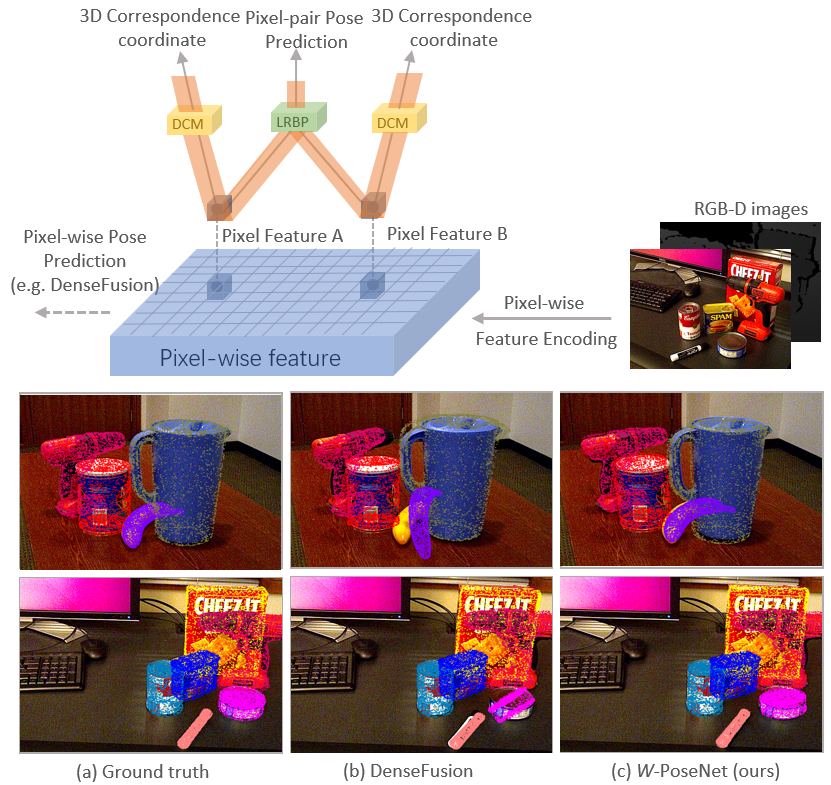
Figure 1: Visualization of our $\mathcal{W}$-PoseNet in comparison with its competitor DenseFusion [14]. The key differences lie in that our $\mathcal{W}$-PoseNet introduces pixel pair pose estimation based on a low-rank bilinear pooling (LRBP, highlighted in a green block) and dense correspondence mapping (DCM) from each pixel to its 3D coordinate (highlighted in yellow blocks), whose geometric structure is similar to the font $\mathcal{W}$ highlighted in orange. Illustrative examples at the bottom rows are from the YCB-Video [10].

On one hand, beyond one loss term as other pixel-wise pose regressors [14, 15] on minimizing pose predictions and their corresponding ground truth, the proposed $\mathcal{W}$-PoseNet additionally encodes the textural and geometric information favoring for reconstructing pose-sensitive point sets, whose points’ 3D coordinates are generated by transforming the observed point cloud sampling from object models (e.g. CAD models) with the inverse of ground truth pose. In detail, our $\mathcal{W}$-PoseNet incorporates an auxiliary task of dense correspondence mapping from each pixel of input data to its corresponding coordinate in the canonical space, in order to regularize local feature learning for pose regression by extra pixel-wise supervision self-generated from object models and ground truth pose. Intuitively, compared to sparse semantic keypoints pre-defined in keypoint-based methods [16, 17, 18, 19, 20], dense correspondence mapping in our scheme treats each pixel as a keypoint to regress its corresponding 3D coordinate in object model space, which makes each pixel-wise feature more discriminative, and thus our pixel-wise feature encoding is more robust to occlusion.

On the other hand, inspired by the point-pair feature [21, 22] on point clouds, this paper proposes a novel pixel pair feature encoding layer based on the low-rank bilinear pooling [23, 24] to generate pixel-pair features from two sampled pixels’ vectors in feature map output of the encoder, which are then mapped onto 6-DoF pose. Similar to the concept in [21, 22], our pixel-pair features describe the relative geometric structure of two sampled 3D points on the object models, but also contain texture information of their 2D projection on input RGB images. Moreover, local features anchored on single pixels concern on extracting textural and geometric information in local regions, which can be less discriminative to some symmetric poses. Such an observation encourages our motivation to combine pixel-wise features into a set of pixel-pair features. A global representation for each instance, which combines a number of pixel-pairs’ features, thus generates a pose prediction.

The main contributions of this paper are three-fold.

• This paper is the first attempt to introduce the concept of a pair-wise combination of dense features to 6D pose estimation. To this end, this paper proposes a novel pixel-pair pose regression network – $\mathcal{W}$-PoseNet, which aims to learn a global representation of each object instance consisting of sparse pixel-pair features (PiPF).

• This paper designs an auxiliary task of dense correspondence mapping from input data to 3D coordinates in object model space sensitive to 6D pose, which can regularize feature encoding in deep pose regression to improve pixel-wise local feature discrimination.

• Extensive experiments are conducted on the popular benchmarks, whose results can demonstrate that the proposed $\mathcal{W}$-PoseNet consistently outperforms the state-of-the-art 6D pose estimation algorithms.

Source codes and pre-trained models will be released after acceptance at https://github.com/xzlscut/W-PoseNet.

II Related Works

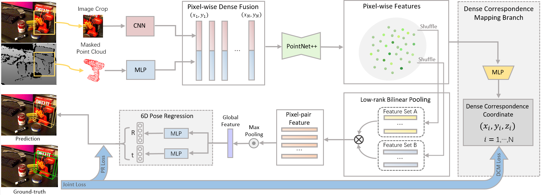
Figure 2: Pipeline of the proposed $\mathcal{W}$-PoseNet. The method first detects and segments the foreground containing object instances on RGB images. RGB and depth images are respectively fed into feature encoders and then fused with the PointNet++ [25]. Pixel-wise features are sparsely sampled and combined to generate pixel pair features, which produce 6D pose $[\bm{R}|\bm{t}]$. The branch about Dense Correspondence Mapping is to regress pose-specific 3D coordinates from per-pixel features, providing additional geometric constraints for feature learning. A joint loss on dense correspondence mapping and pixel-pair pose regression branches are used to supervise network training.

Keypoint-based 6D Pose Estimation – The algorithms belonging to keypoint-based pose estimation share a two-stage pipeline: first localizing 2D projection of predefined 3D keypoints and then generate pose predictions via 2D-to-3D keypoint correspondence mapping with a PnP [26]. Existing methods can be categorized into two groups: object detection based [19, 27] and dense heatmap based [17, 18]. The former focuses on solving the problem of sparse keypoint localization via object detection on the whole object to reduce negative effects of background [19, 27], but are sensitive to occlusion [17]. The latter group of methods [17, 18] pay more attention to discovering latent correlation across all the keypoints and thus are more robust to inter-object occlusion. Recently, PVNet [20] is proposed to detect keypoints via voting on pixel-wise predictions of the directional vector that points to keypoints and is robust to truncation and occlusion. In contrast, dense correspondence mapping in our method share similar concepts as keypoint-based methods but makes pixel-wise predictions on 3D keypoints directly instead of their projection in 2D images, which performs robustly to handle with occlusion.

Dense 6D Pose Estimation – An alternative group of algorithms is to produce dense pose predictions for each pixel or local patches with hand-crafted features [28, 29], CNN patch-based feature encoding [30, 8] and CNN pixel-based feature encoding [14, 15], whose final pose output is selected via a voting scheme. In [31, 32], random forests are adopted to regress 3d coordinates for each pixel and discover 2D-3D correspondence to produce pose predictions. The proposed $\mathcal{W}$-PoseNet is designed to both predict poses from dense features and generate pose-sensitive coordinates in a unique framework. In general, the dense feature encoding module in our method follows the same pipeline as [14, 15], but the key difference lies in incorporating an extra branch to constrain feature encoding with dense correspondence mapping from input data to its corresponding 3D coordinates in a canonical space.

Bilinear Pooling in CNNs – The bilinear pooling [33] is an effective tool to calculate second-order statistics of local features in visual recognition but suffers from expensive computational cost due to its high-dimensionality. A number of its variants have been proposed to cope with the challenge via approximation with Random Maclaurin [34] or Tensor Sketch [35]. A low-rank bilinear model is proposed by Kong et al. [23] to avoid computing the bilinear feature matrix, which is approximated via two decomposed low-rank matrices. Similarly, [24] introduces Grassmann Pooling based on SVD decomposition to approximate feature maps. A quadratic transformation with the low-rank constraint is exploited on pairwise feature interaction either from spatial locations [36] or from feature maps across network layers [37]. Our pixel-pair pose regression shares a similar concept as bilinear models to construct pair-wise features, but a sparsely sampled set of pixel-pair features in $\mathcal{W}$-PoseNet can achieve more robust estimation, owing to the pair-wise combination of spatially localized features.

III Methodology

The problem of 6D pose estimation given RGB-D images is to detect object instances in the scenes and estimate their rotation $\bm{R}\in SO(3)$ and translation $\bm{t}\in\mathbb{R}^{3}$. In detail, a 6D pose can be defined as a rigid transformation $\bm{p}=[\bm{R}|\bm{t}]$ from the object coordinate system with respect to the camera coordinate system. This paper aims to improve the discrimination and robustness of a global representation of each object instance having large variations of texture and shape, from the perspective of pairwise feature interaction on dense local features.

Fig. 2 illustrates the whole pipeline of our $\mathcal{W}$-PoseNet, which consists of several main stages in addition to iterative pose refinement as DenseFusion [14] (see Sec. III-D). Encouraged by the recent success of dense pose regression on RGB-D data, we employ the same feature encoding and fusion part of DenseFusion [14] to extract and fuse pixel-wise features from heterogeneous data (see Sec. III-A). Pixel-wise features are sampled to generate a sparse set of pixel-pair features via a low-rank bilinear pooling on local features, which produces a global feature via a max pooling and its pose prediction (see Sec. III-B). For robust pixel-wise features, an auxiliary task of learning a dense correspondence mapping from each pixel to its 3D coordinate together with pixel-pair pose regression is designed in Sec. III-C. For testing, given an input RGB-D image, the proposed $\mathcal{W}$-PoseNet produces a pose prediction, which as the output of our $\mathcal{W}$-PoseNet is then fed into the iterative pose refinement network to generate a final pose prediction.

III-A Semantic Segmentation and Pixel-Wise Feature Encoding

We adopt the identical modules of the DenseFusion [14] and briefly introduce the following steps: 1) semantic segmentation on RGB images and point clouds converted by depth images; 2) dense feature extraction and 3) pixel-wise feature fusion, which is shown in the top row of Fig. 2.

Following the segmentation algorithm adopted in [14, 10], an RGB image is first fed into the autoencoder-based segmentation network to produce $N+1$ binary masks belonging to $N$ object classes and the background class respectively. The bounding box of each mask is used to crop the corresponding depth image, and the depth intensities within the object mask are converted to a point cloud.

Cropped image patches and point clouds are fed into 2D CNN based and PointNet [38] based feature encoders to respectively extract texture and geometric features from heterogeneous data sources. Specifically, given $H\times W$ RGB-D images, the texture branch aims to mapping $H\times W\times 3$ images to $H\times W\times d_{\text{rgb}}$-dimensional feature maps, which correspond to a feature vector $\bm{f}\in\mathbb{R}^{d_{\text{rgb}}}$ at each spatially localized pixel. The other branch extracts geometric features $\bm{g}$ from orderless points via two shared-MLP and produces $P\times d_{\text{depth}}$-dimensional feature maps where $P$ denotes the size of sampled points in point cloud generated from the depth image.

We combine textural features $\bm{f}$ from those pixels in cropped RGB image patches corresponding to these $P$ points with $\bm{g}$ in the manner of pixel-wise fusion. Specifically speaking, to capture correlation across RGB and depth modalities, geometric and appearance features belonging to the same pixels are first concatenated and then fed into a MLP-based feature fusion network (i.e. PointNet++ [25]) to generate $P$ pixel-wise fusion feature $\bm{x}\in\mathbb{R}^{d_{\text{fusion}}}$. Instead of concatenating the fused feature with a global feature obtained by average pooling as in the DenseFusion[14], we adopted the hierarchical pooling of PointNet++ [25] to aggregate local neighboring features. Our motivation for not using global features here is to get rid of the global information about object instances to verify the effectiveness of a combination of local features as a global description.

III-B Pixel Pair Pose Regression

This section presents the key components of our pixel-pair pose regression: 1) pixel-pair feature generation; 2) pixel-pair feature encoding; and 3) pose regression, which are shown in the bottom row of Fig. 2.

The seminal work of point-pair feature (PPF) [21] constructs 4-dimensional features of a relative position in the manner of Euclidean distance and relative angles between normals and between normals and the determined line from a pair of oriented points sampled from an observed 3D scene. Motivated from its elegant design that can precisely determine a pose when the pair of points is sampled from the object of interest, we propose to pair-wisely aggregate the learned pixel-wise features for a pixel-pair feature encoding (PiPE) to alleviate the suffering of dense features from ambiguities caused by pose symmetries and occlusion.

Generation on Pixel Pair Features – In 3D domain, local descriptors for point clouds can encode the neighboring geometric structure of each point but suffer from sensor noises and sparse point distribution. In view of this, multiple point-pair features [21] consisting of relative position and orientation of two oriented points, are collected as a global representation of an object model. Such a feature representation can still perform robustly to occlusion and sparse point clouds, which is widely adopted for practical applications. Inspired by the robustness and low computational cost of point-pair features [21], we introduce a novel feature encoding layer inserted between the pose regression module and feature fusion module investigated in the previous section. Specifically, given the set $\{\bm{x}\}^{P}$ of $P$ pixel-wise features, we replicate the features into another set. Each feature vector in one set is combined with one randomly selected from the other set, then the $P$ pixels will eventually generate $P$ pixel-pairs. Other combination strategies such as dense pair generation by combining any two pixels can also be employed, but we adopt such a sparse generation owing to its computational simplicity.

Pixel-Pair Feature Encoding (PiPE) – Given the output of pixel pairs, a naive approach to combine local features (i.e., $\bm{x}_{k}$ where $k=1,2,\ldots,P$) into a compact one is direct concatenation, which reveals the 1-order statistical information of local features. An alternative to exploit 1-order statistical information is to generate an element-wise sum of two feature vectors. Encouraged by bilinear models in visual recognition [34, 35, 24], our pixel-pair feature encoding is designed based on a low-rank bilinear pooling [39]. Specifically, given two pixel-wise feature vectors (e.g. $\bm{a}$ and $\bm{b}$ from the set $\{\bm{x}\}^{P}$), the second-order pooling method [40] can be written as

$$\mathcal{G}_{\text{PiPE}}(\bm{a},\bm{b})=\text{vec}(\bm{a}\bm{b}^{T})\in\mathbb{R}^{d_{\text{fusion}}^{2}}.$$ (1)

In view of high-dimensionality $d_{\text{fusion}}^{2}$ of $\bm{a}\bm{b}^{T}$, the low-rank bilinear pooling [39] can be adopted to obtain two low-rank matrices $\bm{U}\in\mathbb{R}^{d_{\text{fusion}}\times l}$ and $\bm{V}\in\mathbb{R}^{d_{\text{fusion}}\times l}$ to avoid computing $\bm{a}\bm{b}^{T}$ as

$$\mathcal{G}_{\text{PiPE}}(\mathbf{a},\mathbf{b})=\bm{P}^{T}\sigma(\bm{U}^{T}\bm{a}\circ\bm{V}^{T}\bm{b})$$ (2)

where $\circ$ denotes the Hadamard product, $\bm{P}$ is the project matrix to determine the output dimension, and we follow [39] use the relu nonlinearity activation function $\sigma(\cdot)$. For generating a $d_{\text{fusion}}$-dimensional pixel-pair feature (the setting in our experiments for a fair comparison), we compare computational complexities of direct concatenation and projection via a fully-connected layer ($2\times d_{\text{fusion}}$, $d_{\text{fusion}}$) and a low-rank bilinear pooling. The former desires $2\times d_{\text{fusion}}^{2}$ network parameters, while the latter needs $3\times d_{\text{fusion}}\times l$ where $l$ denoting the dimension of the compressed vector projected from $\bm{x}$ is usually much smaller than $d_{\text{fusion}}$. As a result, our method adopts the low-rank bilinear pooling in view of the lighter computational cost and the more richer information than direct concatenation, which is verified in our experiments.

Pixel-Pair Pose Regression – All $P$ pixel-pair features $\mathcal{G}_{\text{ppf}}$ are fed into a max pooling to generate a global representation for 6D pose prediction of each object instance. Specifically, the error of pose predictions of the global representation as follows [14]:

$$L_{\text{PR}}=\frac{1}{M}\sum_{j}||(\bm{R}x_{j}+\bm{t})-(\hat{\bm{R}}x_{j}+\hat{\bm{t}})||,$$ (3)

where $x_{j}$ denotes the $j$-th point in a point set randomly sampled from the object model, $M$ is the size of the point set, $[\bm{R}|\bm{t}]$ is the ground-truth pose and $[\bm{\hat{R}}|\bm{\hat{t}}]$ is the predicted pose output by the pixel-pair feature.

III-C Auxiliary Dense Correspondence Mapping

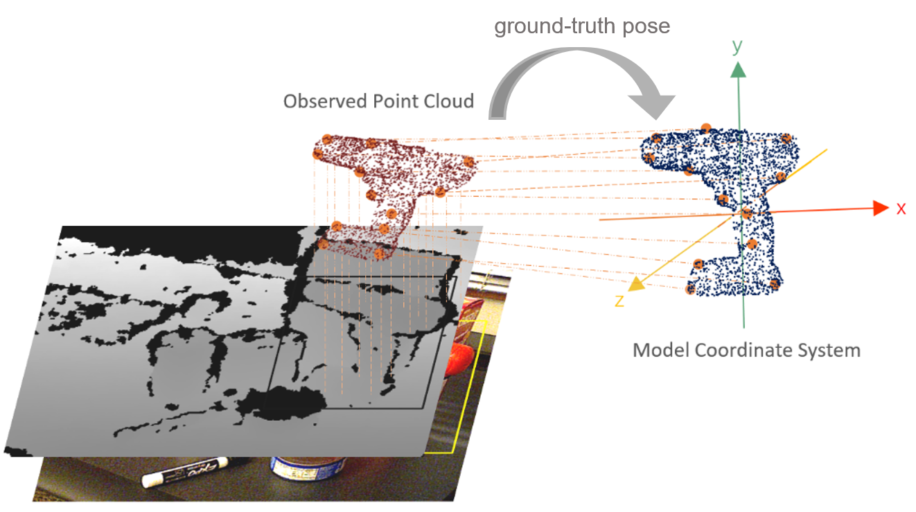
Figure 3: Dense Correspondence Mapping (DCM). This module aims to regularizing feature learning in pose regression with mapping onto 3D coordinates sensitive to 6D poses. Specifically, the point cloud in blue is generated by transforming the point clouds sampled from depth image into the model coordinate system, which are used as supervision signals in DCM.

For obtaining discriminative and robust features per pixels, our method designs an auxiliary dense correspondence mapping task to regularize feature learning. As shown in Fig. 3, dense correspondence mapping is achieved via regressing per-pixel features $\bm{x}$ to its corresponding 3D coordinate in the canonical coordinate system. To this goal, the object point cloud obtained by a depth input image is firstly transformed with the inverse of ground truth pose $[\bm{R}|\bm{t}]$ to obtain its corresponding point cloud in the canonical space. Each 3D coordinate in the transformed point cloud is used as a pixel-wise supervision of its corresponding point in the dense correspondence mapping branch. The loss term on this auxiliary branch, termed as a Dense Correspondence Mapping (DCM) Loss, can be thus written as

$$L_{\text{DCM}}=\frac{1}{M}\sum_{i}||p_{i}-\hat{p}_{i}||$$ (4)

where $M$ represents the points sampled from the observed point cloud, $\hat{p}$ is the prediction of the DCM branch of our network, and $p$ denotes the ground truth coordinate corresponding to $\hat{p}$. A joint loss $L_{\text{joint}}$ to combine both terms for pose regression and dense correspondence mapping can thus be written as:

$$L_{\text{joint}}=L_{\text{PR}}+\lambda L_{\text{DCM}}$$ (5)

where $\lambda$ is the trade-off parameter between two terms.

III-D Iterative Pose Refinement

Iterative refinement in the DenseFusion [14] has gained significant performance improvement for 6D pose estimation. Similarly, we adopt its identical refinement post-processing to improve final pose predictions, which encodes the resulting point clouds after transformation with previous pose predictions to gradually refining pose in a residual learning manner. Experimental results can demonstrate the boosted performance of the proposed $\mathcal{W}$-PoseNet together with the refinement network.

IV Experiments

TABLE I: Comparative evaluation of 6D pose estimation on the YCB-Video Dataset in terms of the ADDS AUC and ADD(S) AUC metrics. Objects in bold are symmetric. Results are report in units of $\%$.

Method	Without Iterative Refinement						With Iterative Refinement
	PoseCNN [10]		DenseFusion [14]		$\mathcal{W}$-PoseNet		PoseCNN+ICP [10]		DenseFusion [14]		$\mathcal{W}$-PoseNet
	ADDS	ADD(S)	ADDS	ADD(S)	ADDS	ADD(S)	ADDS	ADD(S)	ADDS	ADD(S)	ADDS	ADD(S)
002_master_chef_can	83.9	50.2	95.3	70.7	96.0	82.2	95.8	68.1	96.4	73.2	96.0	84.0
003_cracker_box	76.9	53.1	92.5	86.9	93.0	87.1	92.7	83.4	95.8	94.1	95.5	93.0
004_sugar_box	84.2	68.4	95.1	90.8	96.7	94.9	98.2	97.1	97.6	96.5	97.8	96.8
005_tomato_soup_can	81.0	66.2	93.8	84.7	94.3	89.0	94.5	81.8	94.5	85.5	94.5	89.9
006_mustard_bottle	90.4	81.0	95.8	90.9	97.3	95.6	98.6	98.0	97.3	94.7	98.1	97.5
007_tuna_fish_can	88.0	70.7	95.7	79.6	96.5	80.5	97.1	83.9	97.1	81.9	97.3	81.8
008_pudding_box	79.1	62.7	94.3	89.3	95.1	90.8	97.9	96.6	96.0	93.3	96.6	94.3
009_gelatin_box	87.2	75.2	97.2	95.8	96.9	95.0	98.8	98.1	98.0	96.7	98.5	97.3
010_potted_meat_can	78.5	59.5	89.3	79.6	90.8	78.9	92.7	83.5	90.7	83.6	91.6	80.4
011_banana	86.0	72.3	90.0	76.7	95.8	91.2	97.1	91.9	96.2	83.3	97.2	93.9
019_pitcher_base	77.0	53.3	93.6	87.1	96.3	94.2	97.8	96.9	97.5	96.9	98.3	98.1
021_bleach_cleanser	71.6	50.3	94.4	87.5	95.2	88.6	96.9	92.5	95.9	89.9	96.3	91.8
024_bowl	69.6	69.6	86.0	86.0	94.3	94.3	81.0	81.0	89.5	89.5	96.2	96.2
025_mug	78.2	58.5	95.3	83.8	96.5	89.7	94.9	81.1	96.7	88.9	97.1	91.8
035_power_drill	72.7	55.3	92.1	83.7	95.8	93.1	98.2	97.7	96.0	92.7	97.4	96.2
036_wood_block	64.3	64.3	89.5	89.5	91.5	91.5	87.6	87.6	92.8	92.8	91.7	91.7
037_scissors	56.9	35.8	90.1	77.4	88.0	60.6	91.7	78.4	92.0	77.9	89.7	73.0
040_large_marker	71.7	58.3	95.1	89.1	97.1	91.1	97.2	85.3	97.6	93.0	97.5	90.8
051_large_clamp	50.2	50.2	71.5	71.5	75.7	75.7	75.2	75.2	72.5	72.5	76.1	76.1
052_extra_large_clamp	44.1	44.1	70.2	70.2	73.3	73.3	64.4	64.4	69.9	69.9	74.6	74.6
061_foam_brick	88.0	88.0	92.2	92.2	95.8	95.8	97.2	97.2	92.0	92.0	96.9	96.9
ALL	75.8	59.9	91.2	82.9	93.1	87.1	93.0	85.4	93.2	86.1	94.1	89.3

Datasets – To evaluate $\mathcal{W}$-PoseNet comprehensively, we conduct experiments on two popular benchmarks – the YCB-Video dataset [10] and the LineMOD dataset [41]. The YCB-Video dataset consists of 21 objects with different textures and sizes and has 92 videos in total. Following recent work [10, 14, 15], we adopt 80 videos for training, 2949 keyframes from the other 12 videos for testing, and also used an additional 80,000 synthetic images provided by [10]. For a fair comparison, we used the semantic segmentation mask provided by the PoseCNN in evaluation by following [10, 14]. The LineMOD dataset contains 15,783 images belonging to 13 low-textural objects placed under different cluttered environments suffering from the challenges of occlusion and illumination changes. We follow the prior works [14, 15] use 15% of images for training and use the other 85% of images for testing without using additional synthetic data.

Performance Metrics – We adopt the ADDS and ADD(S) metrics in the YCB-Video dataset following recent work [10, 14] for comparative evaluation. For asymmetric objects, we use the average distance (ADD) between 3D model points transformed by ground-truth poses and predicted poses to measure the pose estimation error. For symmetric objects, the average closest point distance (ADDS) is employed to measure the mean error. 6d pose predictions are considered to be correct if the error is smaller than a predefined threshold, which varies from 0 to 10cm to plot an accuracy-threshold curve to compute the area under the curve (AUC). Similarly, for the LineMOD dataset, we use the ADDS distance for symmetric objects (i.e. eggbox and glue) and the ADD distance for the remaining objects having an asymmetric geometry while taking 10% of the diameter as threshold following [14, 19].

Implementation Details – As the DenseFusion [14], in our experiments, the CNN used for texture feature encoding is composed of Resnet-18 [42] followed by 4 blocks of one up-sampling and one convolution layer as the decoder. RGB and depth images are respectively encoded into 128-dimensional vectors, which are fused into a pixel-wise dense feature $\bm{x}_{\text{fusion}}$. The PointNet++ [25] aggregating pixel-wise features consists of two set abstraction and two feature propagation layers. For training our model, learning rate is set $10^{-4}$ with the Adam optimizer.

IV-A Comparison with State-of-the-art Methods

TABLE II: Comparative evaluation of 6D pose estimation in terms of ADD(S) on the LineMOD dataset. Objects in bold are symmetric. The top group of algorithms only use RGB images as input, while the bottom group uses RGB-D images. Ref. denotes the post-processing refinement. Results are reported in units of $\%$.

Method	ape	ben.	cam	can	cat	drill.	duck	egg.	glue	hole.	iron	lamp	phone	MEAN
DeepIM [43]	77.0	97.5	93.5	96.5	82.1	95.0	77.7	97.1	99.4	52.8	98.3	97.5	87.7	88.6
PVNet [20]	43.6	99.9	86.9	95.5	79.3	96.4	52.6	99.2	95.7	82.0	98.9	99.3	92.4	86.3
CDPN [44]	64.4	97.8	91.7	95.9	83.8	96.2	66.8	99.7	99.6	85.8	97.9	97.9	90.8	89.9
Imp.+ICP [11]	20.6	64.3	63.2	76.1	72.0	41.6	32.4	98.6	96.4	49.9	63.1	91.7	71.0	64.7
SSD6D+ICP [12]	65.0	80.0	78.0	86.0	70.0	73.0	66.0	100.0	100.0	49.0	78.0	73.0	79.0	79.0
DenseFusion [14]	79.5	84.2	76.5	86.6	88.8	77.7	76.3	99.9	99.4	79.0	92.1	92.3	88.0	86.2
DenseFusion+Ref. [14]	92.3	93.2	94.4	93.1	96.5	87.0	92.3	99.8	100.0	92.1	97.0	95.3	92.8	94.3
$\mathcal{W}$-PoseNet (ours)	91.7	98.8	98.4	96.5	97.7	96.3	95.0	99.8	99.9	94.4	97.7	99.6	96.8	97.2
$\mathcal{W}$-PoseNet+Ref. (ours)	94.9	98.9	99.1	97.8	98.8	97.1	97.7	99.8	100.0	96.5	97.9	99.3	97.6	98.1

We compare the proposed $\mathcal{W}$-PoseNet and the state-of-the-art methods on the YCB-Video and the LineMOD datasets, and the results are visualized in Tables I and II. In general, our method can consistently achieve state-of-the-art performance with and without iterative pose refinement on the YCB-Video and LineMOD. Specifically, on the YCB-Video, our network consistently performs better than its direct competitor DenseFusion especially for asymmetric objects with and without post-processing refinement, while similar results are observed on the LineMOD dataset. As the dense feature extraction and fusion part of our $\mathcal{W}$-PoseNet and DenseFusion are identical, the performance gain can only be explained by our design on a pixel-pair combination of local features and auxiliary dense correspondence mapping.

Figure 4: Comparison of our $\mathcal{W}$-PoseNet and two state-of-the-art methods under different degree of occlusion.

To verify the robustness of $\mathcal{W}$-PoseNet against inter-object occlusion, we first calculate the invisible surface percentage for each object instance on the YCB-Video dataset as the DenseFusion [14] did, then evaluate the proposed $\mathcal{W}$-PoseNet with different degrees of occlusion. Specifically, we sampled a certain number of points on object models, projected these points onto their image plane by using the ground-truth poses and the camera intrinsic parameters. Given the observation (i.e. depth $d(p)$ on each pixel) in depth images and 2D projection $d(\hat{p})$ of 3D coordinates, if any pixel satisfying $|d(p)-d(\hat{p})|\textgreater{}h$ ($h$ is set to 2cm in our experiment), the pixel is considered under occlusion and can be marked as an invisible pixel. The invisible surface percentage for each instance can be generated via the ratio between the size of invisible points and the total number of sampled points. Fig. 4 shows comparative evaluation of several methods in terms of the ADD(S) metric. Our $\mathcal{W}$-PoseNet can consistently outperform the PoseCNN+ICP [10] and the DenseFusion [14] with increasing the invisible surface percentage. On one hand, both $\mathcal{W}$-PoseNet and DenseFusion are more robust than the PoseCNN+ICP against inter-object occlusion in view of dense feature encoding. On the other hand, the performance gain of our $\mathcal{W}$-PoseNet sharing the identical feature encoding module of the DenseFusion can demonstrate its superior robustness of our dense correspondence regularized pixel pair pose regression to pixel-wise regression in the DenseFusion.

IV-B Ablation Studies

In order to verify the effectiveness of each module of $\mathcal{W}$-PoseNet, we conducted a number of ablation experiments on the LineMOD dataset without iterative pose refinement.

Effects of Pixel-Pair Pose Prediction – Compared to pixel-wise pose estimation in the DenseFusion [14], our $\mathcal{W}$-PoseNet without the DCM Loss and post-refining gain 88.2% on the mean ADD(S), while the DenseFusion without refinement can only achieve 86.2%. The only difference between $\mathcal{W}$-PoseNet without the DCM Loss and the DenseFusion lies in the usage of pixel-pair pose regression, and thus 2% improvement gain can be credited to the effects of Pixel-Pair Pose Prediction.

Evaluation on the DCM Loss – We compare the DenseFusion and our $\mathcal{W}$-PoseNet without pixel-pair regression, obtaining 86.2% and 93.2% respectively, which only differ on the usage of additional dense correspondence mapping branch. It is evident that, owing to introducing the auxiliary DCM branch, the $\mathcal{W}$-PoseNet can significantly outperform the state-of-the-art DenseFusion by 7%, which indicates that the DCM branch improves the quality of per-pixel features.

TABLE III: Ablation studies about combination of local features in terms of ADD(S). Results are report in units of $\%$.

	ELS	CON	LRBP	DCM+ELS	DCM+CON	DCM+LRBP
ADD(S)	91.4	92.5	92.8	96.0	97.0	97.2

Effects of the Feature Fusion Module – We explore a variety of feature fusion methods, including the element-wise sum (ELS), direct concatenation (CON), and low-rank bilinear pooling (LRBP) under two settings, i.e. with and without the auxiliary correspondence mapping (DCM). Among these methods, the LRBP consistently achieves the best performance in both settings. Such a study verifies the efficacy of a bilinear pooling to exploit the richer 2-order statistics of local features.

Effects of Iterative Pose Refinement – We employ the identical refinement network with the same settings as the DenseFusion. From Tables I and II, iterative pose refinement can further boost estimation performance of our $\mathcal{W}$-PoseNet.

V Conclusions

This paper introduces a novel 6D pose estimation network based on two key observations: extracting discriminative dense features in local regions and generating a robust global representation of each object instance. To this end, we introduce two novel modules into the state-of-the-art DenseFusion – pixel-pair pose prediction and dense corresponding mapping utilizing object models, which are verified their effectiveness in the experiments respectively.

References

- [1] E. Marchand, H. Uchiyama, and F. Spindler, “Pose estimation for augmented reality: a hands-on survey,” TVCG, 2015.
- [2] Y. K. Yu, K. H. Wong, and M. M.-Y. Chang, “Pose estimation for augmented reality applications using genetic algorithm,” IEEE Transactions on Systems, Man, and Cybernetics, Part B (Cybernetics), 2005.
- [3] J. Tremblay, T. To, B. Sundaralingam, Y. Xiang, D. Fox, and S. Birchfield, “Deep object pose estimation for semantic robotic grasping of household objects,” arXiv preprint arXiv:1809.10790, 2018.
- [4] A. ten Pas, M. Gualtieri, K. Saenko, and R. Platt, “Grasp pose detection in point clouds,” IJRR, 2017.
- [5] M. Zhu, K. G. Derpanis, Y. Yang, S. Brahmbhatt, M. Zhang, C. Phillips, M. Lecce, and K. Daniilidis, “Single image 3d object detection and pose estimation for grasping,” in ICRA, 2014.
- [6] D. Xu, D. Anguelov, and A. Jain, “Pointfusion: Deep sensor fusion for 3d bounding box estimation,” in CVPR, 2018.
- [7] A. Tejani, D. Tang, R. Kouskouridas, and T.-K. Kim, “Latent-class hough forests for 3d object detection and pose estimation,” in ECCV, 2014.
- [8] W. Kehl, F. Milletari, F. Tombari, S. Ilic, and N. Navab, “Deep learning of local rgb-d patches for 3d object detection and 6d pose estimation,” in ECCV, 2016.
- [9] L. Tang, K. Chen, C. Wu, Y. Hong, K. Jia, and Z. Yang, “Improving semantic analysis on point clouds via auxiliary supervision of local geometric priors,” arXiv preprint arXiv:2001.04803, 2020.
- [10] Y. Xiang, T. Schmidt, V. Narayanan, and D. Fox, “Posecnn: A convolutional neural network for 6d object pose estimation in cluttered scenes,” arXiv preprint arXiv:1711.00199, 2017.
- [11] M. Sundermeyer, Z.-C. Marton, M. Durner, M. Brucker, and R. Triebel, “Implicit 3d orientation learning for 6d object detection from rgb images,” in ECCV, 2018.
- [12] W. Kehl, F. Manhardt, F. Tombari, S. Ilic, and N. Navab, “Ssd-6d: Making rgb-based 3d detection and 6d pose estimation great again,” in ICCV, 2017.
- [13] P. Besl and N. D. McKay, “A method for registration of 3-d shapes,” TPAMI, 1992.
- [14] C. Wang, D. Xu, Y. Zhu, R. Martín-Martín, C. Lu, L. Fei-Fei, and S. Savarese, “Densefusion: 6d object pose estimation by iterative dense fusion,” in CVPR, 2019.
- [15] Y. Cheng, H. Zhu, C. Acar, W. Jing, Y. Wu, L. Li, C. Tan, and J.-H. Lim, “6d pose estimation with correlation fusion,” arXiv preprint arXiv:1909.12936, 2019.
- [16] A. Newell, K. Yang, and J. Deng, “Stacked hourglass networks for human pose estimation,” in ECCV, 2016.
- [17] M. Oberweger, M. Rad, and V. Lepetit, “Making deep heatmaps robust to partial occlusions for 3d object pose estimation,” in ECCV, 2018.
- [18] G. Pavlakos, X. Zhou, A. Chan, K. G. Derpanis, and K. Daniilidis, “6-dof object pose from semantic keypoints,” in ICRA, 2017.
- [19] M. Rad and V. Lepetit, “Bb8: A scalable, accurate, robust to partial occlusion method for predicting the 3d poses of challenging objects without using depth,” in ICCV, 2017.
- [20] S. Peng, Y. Liu, Q. Huang, X. Zhou, and H. Bao, “Pvnet: Pixel-wise voting network for 6dof pose estimation,” in CVPR, 2019.
- [21] B. Drost, M. Ulrich, N. Navab, and S. Ilic, “Model globally, match locally: Efficient and robust 3d object recognition,” in CVPR, 2010.
- [22] S. Hinterstoisser, V. Lepetit, N. Rajkumar, and K. Konolige, “Going further with point pair features,” in ECCV, 2016.
- [23] S. Kong and C. Fowlkes, “Low-rank bilinear pooling for fine-grained classification,” in CVPR, 2017.
- [24] X. Wei, Y. Zhang, Y. Gong, J. Zhang, and N. Zheng, “Grassmann pooling as compact homogeneous bilinear pooling for fine-grained visual classification,” in ECCV, 2018.
- [25] C. R. Qi, L. Yi, H. Su, and L. J. Guibas, “Pointnet++: Deep hierarchical feature learning on point sets in a metric space,” in NIPS, 2017.
- [26] M. A. Fischler and R. C. Bolles, “Random sample consensus: a paradigm for model fitting with applications to image analysis and automated cartography,” Communications of the ACM, 1981.
- [27] B. Tekin, S. N. Sinha, and P. Fua, “Real-time seamless single shot 6d object pose prediction,” in CVPR, 2018.
- [28] J. Liebelt, C. Schmid, and K. Schertler, “independent object class detection using 3d feature maps,” in CVPR, 2008.
- [29] M. Sun, G. Bradski, B.-X. Xu, and S. Savarese, “Depth-encoded hough voting for joint object detection and shape recovery,” in ECCV, 2010.
- [30] A. Doumanoglou, R. Kouskouridas, S. Malassiotis, and T.-K. Kim, “Recovering 6d object pose and predicting next-best-view in the crowd,” in CVPR, 2016.
- [31] E. Brachmann, A. Krull, F. Michel, S. Gumhold, J. Shotton, and C. Rother, “Learning 6d object pose estimation using 3d object coordinates,” in ECCV, 2014.
- [32] F. Michel, A. Kirillov, E. Brachmann, A. Krull, S. Gumhold, B. Savchynskyy, and C. Rother, “Global hypothesis generation for 6d object pose estimation,” in CVPR, 2017.
- [33] T.-Y. Lin, A. RoyChowdhury, and S. Maji, “Bilinear cnn models for fine-grained visual recognition,” in ICCV, 2015.
- [34] P. Kar and H. Karnick, “Random feature maps for dot product kernels,” in AISTATS, 2012.
- [35] N. Pham and R. Pagh, “Fast and scalable polynomial kernels via explicit feature maps,” in SIGKDD, 2013.
- [36] Y. Li, N. Wang, J. Liu, and X. Hou, “Factorized bilinear models for image recognition,” in ICCV, 2017.
- [37] C. Yu, X. Zhao, Q. Zheng, P. Zhang, and X. You, “Hierarchical bilinear pooling for fine-grained visual recognition,” in ECCV, 2018.
- [38] C. R. Qi, H. Su, K. Mo, and L. J. Guibas, “Pointnet: Deep learning on point sets for 3d classification and segmentation,” in CVPR, 2017.
- [39] J.-H. Kim, K.-W. On, W. Lim, J. Kim, J.-W. Ha, and B.-T. Zhang, “Hadamard product for low-rank bilinear pooling,” 2016.
- [40] J. Carreira, R. Caseiro, J. Batista, and C. Sminchisescu, “Semantic segmentation with second-order pooling,” in ECCV, 2012.
- [41] S. Hinterstoisser, S. Holzer, C. Cagniart, S. Ilic, K. Konolige, N. Navab, and V. Lepetit, “Multimodal templates for real-time detection of texture-less objects in heavily cluttered scenes,” in ICCV, 2011.
- [42] K. He, X. Zhang, S. Ren, and J. Sun, “Deep residual learning for image recognition,” in CVPR, 2016.
- [43] Y. Li, G. Wang, X. Ji, Y. Xiang, and D. Fox, “Deepim: Deep iterative matching for 6d pose estimation,” in European Conference on Computer Vision (ECCV), 2018.
- [44] Z. Li, G. Wang, and X. Ji, “Cdpn: Coordinates-based disentangled pose network for real-time rgb-based 6-dof object pose estimation,” in Proceedings of the IEEE International Conference on Computer Vision, 2019, pp. 7678–7687.