Heat flow and noncommutative quantum mechanics in phase-space

Abstract

The complete understanding of thermodynamic processes in quantum scales is paramount to develop theoretical models encompassing a broad class of phenomena as well as to design new technological devices in which quantum aspects can be useful in areas as quantum information and quantum computation. Among several quantum effects, the phase-space noncommutativity, which arises due to a deformed Heisenberg-Weyl algebra, is of fundamental relevance in quantum systems where quantum signatures and high energy physics play important roles. In low energy physics, however, it may be relevant to address how a quantum deformed algebra could influence some general thermodynamic protocols, employing the well-know noncommutative quantum mechanics in phase-space. In this work, we investigate the heat flow of two interacting quantum systems in the perspective of noncommutativity phase-space effects and show that by controlling the new constants introduced in the quantum theory the heat flow from the hot to the cold system may be enhanced, thus decreasing the time required to reach thermal equilibrium. We also give a brief discussion on the robustness of the second law of thermodynamics in the context of noncommutative quantum mechanics.

I Introduction

Quantum thermodynamics comprises the energy conversion in a scale where quantum effects may be useful to improve some specific protocol. It is expected that advances in quantum thermodynamics will be useful in many fundamental aspects as well as in a vast range of technological applications, such as quantum information and quantum communication (Adesso, ; Wang, ), quantum cryptography (Adesso02, ; Yang2019, ; Dowling2015, ), quantum computation (Chuangbook, ; Googlepaper2019, ; Wright2019, ), and in the development of different models of quantum heat machines (Camati2019, ; Kosloff2019, ; Paternostro2019, ; key-9, ; Klatzow2019, ; Santos2018, ; Camati2020, ). In continuous variable systems, a considerable number of platforms have been suitable for testing the laws of thermodynamics in the quantum limit, such as quantum optics (Reiter, ; Haroche2001, ; Walls, ), optomechanical devices (Zhang2014, ; Kampel2013, ; Clerk2013, ), and trapped ions (Sage2019-1, ). Furthermore, supporting the thermal interaction between two general systems, there is a basic statement claiming that for initially uncorrelated systems heat naturally flows from the hotter to the colder system, well know how Clausius statement (Clausius, ). Another particularly interesting scenario in which the heat flow has been addressed consist in a chain of coupled harmonic oscillators where the first and last are in contact with thermal reservoirs in distinct temperatures (Oliveira2017, ; Casetti2018, ; Dantan2015, ), in cases of several thermal reservoirs in linear quantum lattices (Landi2019, ), and in the presence of time-dependent periodic drivings (Fiore2019, ).

Among relevant quantum effects that have been largely investigated in quantum thermodynamics, such as entanglement (Horodecki2009, ), coherence (Plenio2017, ), non-Markovian behavior (Breuer2016, ) and general quantum correlations (Modi2012, ), from a theoretical point of view stimulating questions arise when features encompassing the context of noncommutative phase-space extension of the quantum mechanics are considered. These questions were firstly addressed in the configuration space by Synder (Snyder, ) as a propose to avoid divergences in the quantum field theory. More recently, with a deep consensus that in the Planck scale $(\ell_{P}=\sqrt{\hbar G/c^{3}}\sim 10^{-35}cm)$ the notion of space-time has to be significantly modified (ref01, ; ref02, ), in order to contemplate general noncommutativity at high energy scales, a large number of works dealing with noncommutative signatures in different scenarios has been reported. In what concerns the conventionally known as noncommutative quantum mechanics (NCQM), there have been many studies dedicated to investigate possible effects and signatures of noncommutativity, for instance, in $2D$-harmonic oscillators (Bernardini01, ; Vergara, ), the gravitational quantum well (Orfeu01, ; Banerjee, ; Gnatenko2019A, ; Lawson2017, ), in relativistic dispersion relations (Leal01, ), and exploring different aspects of quantum information (Jonas2016, ; Leal2018, ; Leal2019, ; Paris2016, ). The influence of noncommutative quantum mechanics has been also analyzed in $\mathcal{PT}$-symmetric Hamiltonians (Giri2009, ; Santos2019A, ; Dey2012, ). Although at present the ability to experimentally access noncommutative signatures has not been reached, some theoretical advances have arisen, e.g. in quantum optics (Dey2017, ) and optomechanical devices (Faizal2018, ).

Due to the extensive domain of quantum thermodynamics (Anders2016, ; Kosloff00, ; Deffner00, ), an interesting fundamental question is how noncommutativity could modify thermodynamics protocols in quantum scales. Motivated by the same issue, noncommutativity has been addressed in some models of quantum heat machines (Jonas02, ; Pandit2019, ; Chattopadhyay2019, ) as well as in dissipative dynamics of Brownian particles (Dias2009, ; Almeida2017, ) and Gaussian states (Santos2019, ). In this work we address the question of how noncommutativity in phase-space could impact the heat flow between two interacting systems with different temperatures. With this purpose, we provide a simple recipe to obtain thermal states of harmonic oscillators that evolve under the action of noncommutative parameters. Then, evolving these interacting thermal states unitarily, we show that the noncommutative effects may be used to enhance the heat flow from the hot to the cold system, i.e. decreasing the time to the two systems reach thermal equilibrium. On theoretical aspects, this work is supported by recent studies concerning quantum effects in the heat flow between interacting systems, for instance, in Ref. (Partovi2008, ; Rudolph2012, ), and by arguments that quantum signatures due to additional noncommutativity are universal (Das2008, ). On the other hand, the experimental implementation of the reversion in the heat flow of two qubits (Serra2019, ) inspires for searching new quantum signatures in quantum thermodynamic processes. Moreover, the use of analog gravity models to simulate general uncertainty has been reported in Ref. (Conti2019, ).

The work is organized as follows. Section II is dedicated to introduce the main properties of noncommutativity in phase-space as well as Gaussian states and heat flow. In section III we discuss formal aspects in considering noncommutative effects during the heat exchange process between two interacting systems. In the following, we study an example of two interacting thermal states of harmonic oscillators discussing the local internal energies and introducing a heating power for the colder system. We conclude and draw final remarks in section IV.

II Theoretical framework

In this section we review the basic theoretical properties of noncommutative quantum mechanics in phase-space and some important tools of quantum thermodynamics and quantum information that will be useful in the following.

II.1 Noncommutative quantum mechanics in phase-space

The noncommutativity of the phase-space is based on the deformed Heisenberg-Weyl algebra (Rojas2001, ; Bastos2008, ; Gouba2010, ; Gouba2016, ) which can be represented by the commutation relations,

$$\left[q_{i},q_{j}\right]=i\theta_{ij},\,\left[q_{i},p_{j}\right]=i\hbar\delta_{ij},\,\left[p_{i},p_{j}\right]=i\eta_{ij},$$ (1)

with $i,j=1,...,d$, $\theta_{ij}$ and $\eta_{ij}$ are invertible antisymmetric real constant $(d\times d)$ matrices, and one can define the matrix $\Sigma_{ij}=\delta_{ij}+\theta_{ik}\eta_{kj}/\hbar^{2}$, which is also invertible if $\theta_{ik}\eta_{kj}\neq-\hbar^{2}\delta_{ij}$. Writing $\theta_{ij}=\theta\epsilon_{ij}$ and $\eta_{ij}=\eta\epsilon_{ij}$, with $\epsilon_{ii}=0$, $\epsilon_{ij}=-\epsilon_{ji}$, one can interpret $\theta$ and $\eta$ as being new constants in the quantum theory, which have been extensively studied recently (Bernardini01, ; Jonas02, ; Saha, ; Bastos, ; Bastos02, ; Andreas, ; Liang2019, ; Bastos2008-1, ). Besides, $\theta$ and $\eta$ are assumed to be positive quantities. Given a quantum system described by the Hilbert space of the NCQM, it is possible to represent it in the context of the standard quantum mechanics (SQM), which is governed by the well-know commutation relations,

$$\left[Q_{i},P_{j}\right]=0,\,\left[Q_{i},P_{j}\right]=i\hbar\delta_{ij},\,\left[P_{i},P_{j}\right]=0.$$ (2)

This is performed through the Seiberg-Witten (SW) map Orfeu02 ; Santos2015 ; Gamboa , given by,

$$q_{i}=\nu Q_{i}-(\theta/2\nu\hbar)\epsilon_{ij}P_{j},\quad p_{i}=\mu P_{i}+(\eta/2\mu\hbar)\epsilon_{ij}Q_{j},$$ (3)

in which $\nu$ and $\mu$ are arbitrary parameters fulfilling the condition $\theta\eta=4\hbar^{2}\mu\nu(1-\mu\nu)$. Thus, for a general quantum system described by the Hamiltonian $H^{nc}(q_{i},p_{i})$ in the NC phase-space, the action of the SW map can be summarized as follows,

$$H^{nc}(q_{i},p_{i}) \longrightarrow\mathcal{H}(Q_{i},P_{i})$$

$$=H(Q_{i},P_{i})+f(\theta,\eta)V(Q_{i},P_{i}),$$ (4)

where $H(Q_{i},P_{i})$ has the same Hamiltonian structure as $H^{nc}(q_{i},p_{i})$, $f(\theta,\eta)$ is a function of the noncommutative parameters, and $V(Q_{i},P_{i})$ is in general an interaction Hamiltonian term.

II.2 Thermal states and heat flow

Thermal states have special relevance in quantum thermodynamics, for instance, they are useful in representing asymptotic states of quantum systems in contact with thermal reservoirs and to build several models of quantum thermal machines. Moreover, they are a particular set of a larger one, well know as Gaussian states which, in its turn, are completely characterized by the first statistical moments and covariance matrix (Adesso, ; Wang, ; Serafini, ). For two-mode Gaussian states, defining a vector $\vec{R}(Q_{1},P_{1},Q_{2},P_{2})$ to group the coordinates of a two-dimensional system, the first moments are defined as the vector $\vec{d}=(\langle Q_{1}\rangle_{\rho},\langle P_{1}\rangle_{\rho},\langle Q_{2}\rangle_{\rho},\langle P_{2}\rangle_{\rho})$. The covariance matrix (CM) is the set of all second statistical moments, given by $\sigma=\sigma_{11}\oplus\sigma_{22}$ for a two-mode Gaussian state, with,

$$\sigma_{ii}=\left(\begin{array}[]{cc}\sigma_{Q_{i}Q_{i}}&\sigma_{P_{i}Q_{i}}\\ \sigma_{Q_{i}P_{i}}&\sigma_{P_{i}P_{i}}\end{array}\right),$$ (5)

where $\sigma_{\alpha\beta}=\langle\alpha\beta+\beta\alpha\rangle_{\rho}-2\langle\alpha\rangle_{\rho}\langle\beta\rangle_{\rho}$. For physical two-mode Gaussian states the CM satisfies the relation $\sigma+i\Omega\geq 0$, with,

$$\Omega=\left(\begin{array}[]{cc}0&1\\ -1&0\end{array}\right)^{\oplus 2},$$ (6)

such that $\left[\vec{R}_{i},\vec{R}_{j}\right]=i\Omega_{ij}$ (Simon, ). In special, for Gaussian states the Wigner function assumes a gently form given by (Adesso, ),

$$W_{G}(\vec{R})=\frac{exp\left[-(1/2)(\vec{R}-\vec{d})\sigma^{-1}(\vec{R}-\vec{d})\right]}{(2\pi)^{2n}\sqrt{Det[\sigma]}}.$$ (7)

A one-mode thermal state can be represented by (Adesso, ; Wang, ; Serafini, ),

$$\rho^{th}(\bar{n})=\sum_{n=0}^{\infty}\frac{\bar{n}^{m}}{(\bar{n}+1)^{n+1}}|n\rangle\langle n|,$$ (8)

with $\bar{n}=\left\{\text{exp}\left[\hbar\omega/k_{B}T\right]-1\right\}^{-1}$ the mean number of photons in the bosonic mode, $k_{B}$ is the Boltzmann constant, $T$ is the associated temperature, and $\{|m\rangle\}$ is the Fock basis. It is direct to note that number $\bar{n}$ is proportional to the temperature of a thermal state. The first moments and covariance matrix of a one-mode thermal state are $\vec{R}=(0,0)$ and $\sigma=(2\bar{n}+1)\mathbb{I}_{2\times 2}$, respectively (Adesso, ; Wang, ; Serafini, ).

In quantum thermodynamics, given a quantum system with time-independent Hamiltonian $H$ and state $\rho$, the associated energy is obtained by $U(\rho(t))=\text{Tr}[H\rho(t)]$. For the particular case of Gaussian states with zero first moments, the energy is simply the trace of the covariance matrix, i.e. $U(\rho(t))=\text{$(\hbar\omega/4)$Tr}[\sigma(t)]$ (Adesso, ) (see Appendix A). Considering two quantum systems, $1$ and $2$, under the action of a heat exchange protocol during the time comprised between $[0,\tau]$, the heat exchanged by the system $1$ is given by $\langle Q\rangle_{1}=\text{$(\hbar\omega/4)($Tr}[\sigma(\tau)]-\text{Tr}[\sigma(0)])$ and, as expected, $\langle Q\rangle_{2}=-\langle Q\rangle_{1}$, since the we are assuming a unitary evolution, as illustrated in Fig. 1.

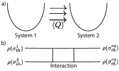
Figure 1: a) Illustration of the heat exchange process in which heat flows from the system 1 to the system 2. b) A simple circuit depicting the interaction between the two systems, initially prepared in local thermal states and achieving thermal equilibrium at the end of the protocol.

III Enhancing the heat flow with nc effects

General formalism

Consider two interacting systems in which the time-independent Hamiltonian $H(q_{i},p_{i})$ is governed by the commutation relations in (1). After implementing the Seiberg-Witten map, the new Hamiltonian is given by $\mathcal{H}(Q_{i},P_{i})$. Assuming that we have initially uncorrelated local thermal states for each system such that, $\rho_{i}^{th}(0)=\text{exp}(-\beta_{i}\hbar\omega_{i})/\text{Tr}[\exp(-\beta_{i}\hbar\omega_{i})]$, after the time evolution the final states are,

$$\rho_{i}^{th}(t)=U_{t,0}^{\theta,\eta}\rho_{i}^{th}(0)\left(U_{t,0}^{\theta,\eta}\right)^{\dagger},$$

with the time-evolution operator given by $U_{t,0}^{\theta,\eta}=\exp[-i\mathcal{H}t/\hbar]$. It is worth to mention that, once the structure of $\mathcal{H}(Q_{i},P_{i})$ is given by Eq. (4), the time evolution of the composite system generates correlations between the parts. The internal energy of each system in time $t$ is $E_{i}(t)=Tr[\rho_{i}^{th}(t)\mathcal{H}]$ which allows to write the heat exchanged during the time evolution, $\langle Q_{i}\rangle=E_{i}(t)-E_{i}(0)$. In the absence of any noncommutative effects, $\theta=\eta=0$, we recover the traditional form of the heat well know in the standard quantum mechanics. However, the existence of any noncommutative effects will be captured in the heat exchanged by the two systems. A more detailed information about the time-evolution operator with NC effects is provided in Appendix B.

Two-interacting oscillators

Here we consider an example of two interacting quantum systems in order to show that the noncommutativity of the phase-space may be used to enhance the heat flow and decrease the time to reach the thermal equilibrium. Consider two-coupled harmonic oscillators described in the NCQM (commutation relations in Eqs (1)) , in which the Hamiltonian reads,

$$H^{nc}(q_{i},p_{i})=\sum_{i=1}^{2}\left(\frac{p_{i}^{2}}{2m}+\frac{m\Omega^{2}}{2}q_{i}^{2}\right)+\frac{\omega_{B}}{2}\sum_{i,j=1}^{2}\epsilon_{ij}p_{i}q_{j,}$$ (9)

with $\Omega^{2}=\omega^{2}+\omega_{B}^{2}/4$, in which $m$ and $\omega$ are the mass and frequency of the oscillators, respectively, and $\omega_{B}$ is the coupling frequency. This type of interaction corresponds, for instance, to a uniform magnetic field applied on the orthogonal direction, being a good approximation of a confinement implemented in semiconductor quantum dots (Jacak1998, ). Once we transform the Hamiltonian in Eq. (9) to the standard quantum mechanics, we obtain,

$$\mathcal{H}(Q_{i},P_{i})=\alpha^{2}Q_{i}^{2}+\beta^{2}P_{i}^{2}+\left(\frac{\omega_{B}}{2}+\gamma\right)\sum_{i,j=1}^{2}\epsilon_{ij}P_{i}Q_{j,}$$ (10)

with the following definitions,

$$\alpha^{2} = \frac{\nu^{2}m\Omega^{2}}{2}+\frac{\eta^{2}}{8m\mu^{2}\hbar^{2}}+\frac{\nu}{\mu}\frac{\omega_{B}\eta}{4\hbar^{2}},$$

$$\beta^{2} = \frac{\mu^{2}}{2m}+\frac{m\Omega^{2}\theta^{2}}{8\nu^{2}\hbar^{2}}+\frac{\mu}{\nu}\frac{\omega_{B}\theta}{4\hbar},$$

$$\gamma = \frac{\theta}{2\hbar}m\Omega^{2}+\frac{\eta}{2m\hbar}.$$

Despite the relative complexity in expressions for $\alpha^{2}$ and $\beta^{2}$, we note that the only effect of these constants on the Hamiltonian is to induce a shift in the position and momentum of the oscillators. The relevant effect is exclusively due to $\gamma$ which depends on the NC parameters and may influence the interaction Hamiltonian,

$$V(Q_{i},P_{i})=\left(\frac{\omega_{B}}{2}+\gamma\right)\sum_{i,j=1}^{2}\epsilon_{ij}P_{i}Q_{j}.$$ (11)

It is important to note that the interaction Hamiltonian commutes with the total Hamiltonian of the two quantum oscillators, $[\alpha^{2}Q_{i}^{2}+\beta^{2}P_{i}^{2},V(Q_{i},P_{i})]=0$, implying that the heat exchange process that we will employ does not perform work. This results that the heat exchanged between the oscillators is constant in time, $\langle Q_{1}\rangle+\langle Q_{2}\rangle=0$, with the internal energy variation, $\Delta E_{i}=\langle Q_{i}\rangle=Tr[\sigma_{i}(\tau)]-Tr[\sigma_{i}(0)]$.

To model the thermal interaction between the two oscillators we consider the initial state preparation developed in Ref. (Bernardini01, ) and with the Wigner function written as,

$$W_{k,\ell}(Q_{i},P_{i})=\frac{(-1)^{k+\ell}}{\pi^{2}\hbar^{2}}\exp\left[-\xi_{1(2)}^{2}/\hbar\right]L_{k(\ell)}^{(0)}\left[2\xi_{1(2)}^{2}/\hbar\right],$$ (12)

with,

$$\xi_{1}^{2} =\left(\frac{\alpha}{\beta}Q_{1}^{2}+\frac{\beta}{\alpha}P_{1}^{2}\right)\cos(\Gamma t)^{2}+\left(\frac{\alpha}{\beta}Q_{2}^{2}+\frac{\beta}{\alpha}P_{2}^{2}\right)\sin(\Gamma t)^{2}$$

$$-\left(\frac{\alpha}{\beta}Q_{1}Q_{2}+\frac{\beta}{\alpha}P_{1}P_{2}\right)\sin(2\Gamma t),$$

$$\xi_{2}^{2} =\left(\frac{\alpha}{\beta}Q_{1}^{2}+\frac{\beta}{\alpha}P_{1}^{2}\right)\sin(\Gamma t)^{2}+\left(\frac{\alpha}{\beta}Q_{2}^{2}+\frac{\beta}{\alpha}Q_{2}^{2}\right)\cos(\Gamma t)^{2}$$

$$+\left(\frac{\alpha}{\beta}Q_{1}Q_{2}+\frac{\beta}{\alpha}P_{1}P_{2}\right)\sin(2\Gamma t),$$

with $k$ and $\ell$ integer numbers and $\Gamma=\omega_{B}/2+\gamma$. Note that the state $W_{k,\ell}(q_{i},p_{i})$ is non-stationary unless $\Gamma=0$, implying no interaction between the oscillators. Then, the role of the noncommutative parameters, mediated by $\gamma$, is to affect the interaction between the systems, as evidenced in Eq. (11). Starting from Eq. (12) we can generate a set of thermal states simply obtaining the covariance matrix from the local states. First, the local states of each oscillator are given by tracing out the other degree of freedom, i.e.,

$$W_{k,\ell}^{1}=W_{k,\ell}^{1}(Q_{1},P_{1}) =\int\int dQ_{2}dP_{2}\,W_{k,\ell}(Q_{i},P_{i}),$$

$$W_{k,\ell}^{2}=W_{k,\ell}^{2}(Q_{2},P_{2}) =\int\int dQ_{1}dP_{1}\,W_{k,\ell}(Q_{i},P_{i}).$$ (13)

From the local states, we then obtain the covariance matrix, just as in Eq. (5), and define the following local thermal states as,

$$\sigma_{th}^{i;k,\ell}(t)=\frac{\hbar\omega}{4}(2\bar{n}+1)\left(\begin{array}[]{cc}\langle Q_{i}Q_{i}\rangle_{W_{k,\ell}^{i}}&\langle Q_{i}P_{i}\rangle_{W_{k,\ell}^{i}}\\ \langle P_{i}Q_{i}\rangle_{W_{k,\ell}^{i}}&\langle P_{i}P_{i}\rangle_{W_{k,\ell}^{i}}\end{array}\right),$$ (14)

with $i=1,2$ and $\bar{n}$ different for each oscillator. We highlight that by construction, we have $\langle Q_{i}P_{i}\rangle_{W_{k,\ell}^{i}}=\langle P_{i}Q_{i}\rangle_{W_{k,\ell}^{i}}=0$ and $\langle Q_{i}Q_{i}\rangle_{W_{k,\ell}^{i}}=\langle P_{i}P_{i}\rangle_{W_{k,\ell}^{i}}$, besides the fact the first moments are zero, characterizing the thermal states. These results are valid irrespective the values of $k$ and $\ell$. It is important to stress that the thermal states generated by these protocol are strictly dependent on the noncommutative parameters $\theta$ and $\eta$. The internal energy associated to each system is given by $E_{i}^{k,\ell}(t)=(\hbar\omega/4)Tr[\sigma_{th}^{i;k,\ell}(t)]$, resulting that the heat exchanging between the two systems is $\langle Q_{1}^{k,\ell}\rangle=-\langle Q_{2}^{k,\ell}\rangle=E_{1}^{k,\ell}(t)-E_{1}^{k,\ell}(0)$.

In order to consider a pair of thermal states to analyze the NC effects on the heat exchange process, we choose the quantum numbers in the state (12) to be $(k,\ell)=(0,1)$, and make the notation simpler by writing $\sigma_{th}^{i;k,\ell}=\sigma_{th}^{i}$. Then, using the protocol to obtain the covariance matrix given in Eq. (14) we get,

$$\sigma_{th}^{1}(t) =\frac{\hbar\omega}{2}(2\bar{n}+1)\left[1-\frac{1}{2}\cos\left(\omega_{B}\left(\frac{\gamma}{\omega_{B}}+\frac{1}{2}\right)t\right)\right]\mathbb{I}_{2\times 2},$$

$$\sigma_{th}^{2}(t) =\frac{\hbar\omega}{4}(2\bar{m}+1)\left[2+\cos\left(\omega_{B}\left(\frac{\gamma}{\omega_{B}}+\frac{1}{2}\right)t\right)\right]\mathbb{I}_{2\times 2}.$$ (15)

Using these covariance matrices for the generated thermal states, we directly obtain the internal energy associated to each oscillator,

$$E_{1}(t) =\hbar\omega(2\bar{n}+1)\left[1-\frac{1}{2}\cos\left(\omega_{B}\left(\frac{\gamma}{\omega_{B}}+\frac{1}{2}\right)t\right)\right],$$

$$E_{2}(t) =\frac{\hbar\omega}{2}(2\bar{m}+1)\left[2+\cos\left(\omega_{B}\left(\frac{\gamma}{\omega_{B}}+\frac{1}{2}\right)t\right)\right].$$ (16)

In Fig. (2) we show the internal energy of the two oscillators during the heat exchange protocol for different values of NC parameters. We have chosen $(\bar{n},\bar{m})=(2,4)$, meaning that the oscillator 2 (red lines) is hotter than the oscillator 1 (blue lines). The case without any NC effects, $\gamma=0$, is represented by the solid lines, whereas we considered two cases with NC effects, $\gamma=0.1$ (dashed lines), and $\gamma=0.5$ (dotted lines). It can be observed that the inclusion of a deformed Heisenberg-Weyl algebra, see Eq. (1), allows to decrease the time required to reach thermal equilibrium. Furthermore, in order to illustrate the initial thermal states given by the covariance matrices in Eq. (15) as well as the thermal states in the thermal equilibrium, we plot in Fig. (3) the corresponding Wigner function. The time to reach thermal equilibrium is found to be $\tau=2\arccos[-2(m-n)/(1+m+n)]/(2\gamma+\omega_{B})$. A similar result is obtained in the case of $(k,\ell)=(1,0)$.

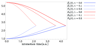
Figure 2: Internal energy of the oscillators 1 (red lines) and 2 (blue lines) as function of the interaction time (arbitrary unities) for different values of $\gamma$, mediating the NC effects. $\gamma=0$ (solid lines), $\gamma=0.1$ (dashed lines), and $\gamma=0.5$ (dotted lines). We have plotted the internal energies for each value of noncommutative parameter up to the corresponding time required to reach thermal equilibrium. It was considered $\hbar=m=k_{B}=\omega_{B}=1$, $\omega=4$ and $(\bar{n},\bar{m})=(2,4)$.

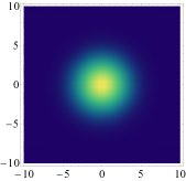
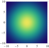
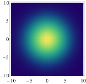
Figure 3: Wigner functions (in $(Q_{i},P_{i})$ coordinates) illustrating the thermal states whose covariance matrices are given by expressions in Eq. (15). On the top we have the initial thermal states for $\sigma_{th}^{1}(0)$ (left) and $\sigma_{th}^{2}(0)$ (right), which do not depend on the NC parameters. The thermal states with the same internal energy after the heat exchange protocol are depicted on the bottom. We have considered $\bar{n}=2$ and $\bar{m}=4$, and a blue-green-yellow color scheme.

To explicitly show how noncommutative effects can enhance the heat exchange process we define a heating power, which is the internal energy variation of the colder system divided by the time to reach thermal equilibrium,

$$\mathcal{P}(t) =\frac{E_{1}(t)-E_{1}(0)}{t}.$$ (17)

Figure 4 presents the heating power as a function of the interaction time for the same parameters used in Fig. (2). It is possible to note that the decrease in the thermal equilibrium time due to noncommutative effects implies in larges values of $\mathcal{P}(t)$.

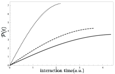
Figure 4: Heating power as a function of the interaction time for the same parameters used in Fig. (2). We have plotted the heating power for each value of noncommutative parameter up to the corresponding time required to reach thermal equilibrium.

Second law of thermodynamics and NC effects

We would like to discuss briefly the possible impacts of the noncommutative parameters on the second law of thermodynamics. For initially uncorrelated two thermal states, with temperatures $T_{2}\geq T_{1}$, or $\bar{n}_{2}\geq\bar{n}_{1}$, a standard way of writing the second law of thermodynamics is given by (Partovi2008, ; Rudolph2012, ),

$$Q_{1}\left(\frac{1}{k_{B}T_{1}}-\frac{1}{k_{B}T_{2}}\right)\geq 0,$$

meaning that heat flows from the hotter to the colder system. For the case we have considered, it is possible to note that the inclusion of new noncommutative relations do not affect the validity of the standard second law of thermodynamics.

IV Conclusions

Quantum thermodynamics has demonstrated its ability in many sectors of physics in quantum scales, experimental and theoretically. Here we have assumed a deformed Heisenberg-Weyl algebra and investigated how the noncommutative parameters $\theta$ and $\eta$ may influence the heat flow of two coupled harmonic oscillators interacting through a heat exchange protocol.

Starting from a general preparation of states proposed in Ref. (Bernardini01, ) whose dynamics is dictated by NC parameters, we provided a scheme for obtaining thermal states that are coupled via the interaction Hamiltonian containing NC effects. Then, since that the interaction Hamiltonian commutes with the total Hamiltonian of the individual systems, it is ensured that all the heat flowing out from the system 2 is absorbed by the system 1. The results shows that noncommutative effects may be employed to enhance the heat flow between the two oscillators, decreasing the time required to reach thermal equilibrium. We highlight that since the noncommutative parameters $\theta$ and $\eta$ are positive quantities, it is not possible to employ it to reverse the heat flow, implying that the standard second law of thermodynamics is robust to the inclusion of new noncommutative relations in the quantum theory. Our results could be used to generate a quantum Otto refrigerator, with NC effects boosting the performance of the quantum fridge.

Although at the moment the technological ability does not allow to experimentally access quantum effects in the Planck scale, our results can be perfectly simulated using some different platforms, such as optomechanical and optical devices. We hope that this work can contribute in this direction, helping to elucidate the role of noncommutative effects in thermodynamic protocols.

V DATA AVAILABILITY

Data sharing is not applicable to this article as no new data were created or analyzed in this study.

Appendix A Energy and covariance matrix for thermal states

Consider a simple quantum harmonic oscillator with frequency $\omega$ and mass $m$ given by,

$$H(Q,P)=\frac{1}{2m}P^{2}+\frac{m\omega^{2}}{2}Q^{2}.$$

The mean value of energy is given by $\langle E\rangle_{\rho}=\langle H\rangle_{\rho}$, with $\rho$ a thermal state. Then,

$$\langle E\rangle_{\rho}=\frac{1}{2m}\langle P\rangle_{\rho}^{2}+\frac{m\omega^{2}}{2}\langle Q\rangle_{\rho}^{2}=\hbar\omega(\langle a^{\dagger}a\rangle_{\rho}+1/2),$$

where $a$ and $a^{\dagger}$ are the annihilation and creation operators, respectively, with $[a,a^{\dagger}]=1$. From (Adesso, ) we have $\langle a^{\dagger}a\rangle_{\rho}=(\text{Tr}[\sigma]-2)/4$, with $\sigma$ the covariance matrix associated to the thermal state $\rho$, $\sigma_{ij}=\langle d_{i}d_{j}+d_{j}d_{i}\rangle_{\rho}-2\langle d_{i}\rangle_{\rho}\langle d_{j}\rangle_{\rho}$ and $\vec{d}=(q,p)$. Thus we have,

$$\langle E\rangle=\frac{\hbar\omega}{4}\text{Tr}[\sigma].$$

Appendix B Time evolution of thermal states with NC effects

Here we provide more details about the time evolution of thermal states with noncommutative effects. Consider that the interaction between the two systems in the noncommutative phase-space coordinates is represented by the Hamiltonian $H_{I}(q_{i},p_{i}).$ After the Seiberg-Witten map, the general interaction reads $g(\theta,\eta)H_{I}(Q_{i},P_{i})+f(\theta,\eta)V(Q_{i},P_{i})$, with $g(\theta,\eta)$ and $f(\theta,\eta)$ real functions such that $g(\theta,\eta)=1$ and $f(\theta,\eta)=0$ in the absence of NC effects. In the interaction picture the time evolution of the local thermal states is given by,

$$\rho_{i}^{th}(t) =U_{t,0}^{\theta,\eta}\rho_{i}^{th}(0)\left(U_{t,0}^{\theta,\eta}\right)^{\dagger},$$

with $U_{t,0}^{\theta,\eta}=\text{exp}[-i(g(\theta,\eta)H_{I}(Q_{i},P_{i})+f(\theta,\eta)V(Q_{i},P_{i}))t/\hbar]$ the time-evolution operator. This expression is general. For $\theta=\eta=0$, the time-evolution operator from the standard quantum mechanics is recovered, otherwise the evolved local thermal states will contain noncommutative signatures.

References

- (1) G. Adesso, S. Ragy, and A. R. Lee, “Continuous variable quantum information: Gaussian states and beyond”, Open Syst. Inf. Dyn., 1440001 (2014). https://doi.org/10.1142/S1230161214400010.
- (2) X. Wang, T. Hiroshima, A. Tomita, and M. Hayashi, “Quantum information with Gaussian states”, Phys. Rep. , 1 (2007). https://doi.org/10.1016/j.physrep.2007.04.005.
- (3) R. Nichols, Pietro Liuzzo-Scorpo, Paul A. Knott, and Gerardo Adesso, “Multiparameter Gaussian quantum metrology”, Phys. Rev. A , 012114 (2018). https://doi.org/10.1103/PhysRevA.98.012114.
- (4) Y. Yang, “Memory effects in quantum metrology”, Phys. Rev. Lett. 123, 110501 (2019). https://doi.org/10.1103/PhysRevLett.123.110501.
- (5) J. P. Dowling and K. P. Seshadreesan, Quantum optical technologies for metrology, sensing and imaging, J. Light. Tech. 33, 2359 (2015). 10.1109/JLT.2014.2386795.
- (6) M. A. Nielsen and I. L. Chuang, “Quantum Computation and Quantum Information”, (Cambridge University Press, Cambridge, 2010). https://doi.org/10.1017/CBO9780511976667.
- (7) F. Arute, K. Arya, R. Babbush, et al., “Quantum supremacy using a programmable superconducting processor”, Nature 574, 505-510 (2019). https://doi.org/10.1038/s41586-019-1666-5.
- (8) K. Wright, K. M. Beck, S. Debnath, et al., “Benchmarking an 11-qubit quantum computer”, Nature Communications 10, 5464 (2019). https://doi.org/10.1038/s41467-019-13534-2.
- (9) P. A. Camati, J. F. G. Santos, and R. M. Serra, “Coherence effects in the performance of the quantum Otto heat engine”, Phys. Rev. A 99, 062103 (2019). https://doi.org/10.1103/PhysRevA.99.062103.
- (10) R. Dann and R. Kosloff, “Quantum Signatures in the Quantum Carnot Cycle”, New J. Phys. 22 013055 (2020). https://doi.org/10.1088/1367-2630/ab6876.
- (11) O. Abah, M. Paternostro, “Implications of non-Markovian dynamics on information-driven engine”, J. Phys. Commun. 4 085016 (2020). https://doi.org/10.1088/2399-6528/abaf99.
- (12) J. P. S. Peterson, T. B. Batalhão, M. Herrera, A. M. Souza, R. S. Sarthour, I. S. Oliveira, R. M. Serra, “Experimental characterization of a spin quantum heat engine”, Phys. Rev. Lett. 123, 240601 (2019). https://doi.org/10.1103/PhysRevLett.123.240601.
- (13) J. Klatzow, J. N. Becker, P. M. Ledingham, et al., “Experimental Demonstration of Quantum Effects in the Operation of Microscopic Heat Engines”, Phys. Rev. Lett. 122, 110601 (2019). https://doi.org/10.1103/PhysRevLett.122.110601.
- (14) J. F. G. Santos, “Gravitational quantum well as an effective quantum heat engine”, Eur. Phys. J. Plus 133, 321 (2018). https://doi.org/10.1140/epjp/i2018-12141-8.
- (15) P. A. Camati, J. F. G. Santos, and R. M. Serra, “Employing Non-Markovian effects to improve the performance of a quantum Otto refrigerator”, Phys. Rev. A 102, 012217 (2020). https://doi.org/10.1103/PhysRevA.102.012217.
- (16) M. J. Kastoryano, F. Reiter, and A. S. Sørensen, “Dissipative Preparation of Entanglement in Optical Cavities”, Phys. Rev. Lett. , 090502 (2011). https://doi.org/10.1103/PhysRevLett.106.090502.
- (17) J. M. Raimond, M. Brune, and S. Haroche, “Colloquium: Manipulating quantum entanglement with atoms and photons in a cavity”, Rev. Mod. Phys. 73, 565 (2001). https://doi.org/10.1103/RevModPhys.73.565.
- (18) D. F. Walls and G. J. Milburn, “Quantum Optics” (Springer, Berlin, 2008). https://doi.org/10.1007/978-3-540-28574-8.
- (19) K. Zhang, F. Bariani, and P. Meystre, “Theory of an optomechanical quantum heat engine”, Phys. Rev. A 90, 023819 (2014). https://doi.org/10.1103/PhysRevA.90.023819.
- (20) T. P. Purdy, P.-L. Yu, R. W. Peterson, N. S. Kampel, and C. A. Regal, “Strong Optomechanical Squeezing of Ligh”, Phys. Rev. X 3, 031012 (2013). https://doi.org/10.1103/PhysRevX.3.031012.
- (21) Ying-Dan Wang and Aashish A. Clerk, “Reservoir-Engineered Entanglement in Optomechanical Systems”, Phys. Rev. Lett. 110, 253601 (2013). https://doi.org/10.1103/PhysRevLett.110.253601.
- (22) .C. D. Bruzewicz, J. Chiaverini, R. McConnell, and J.M. Sage, “Trapped-Ion Quantum Computing: Progress and Challenges”, Appl. Phys. Rev. 6, 021314 (2019). https://doi.org/10.1063/1.5088164.
- (23) R. Clausius, “The Mechanical Theory of Heat” (MacMillan, London, 1879).
- (24) M. J. de Oliveira, “Heat transport along a chain of coupled quantum harmonic oscillators”, Phys. Rev. E 95, 042113 (2017). https://doi.org/10.1103/PhysRevE.95.042113.
- (25) S. Iubini, P. Di Cintio, S. Lepri, R. Livi, and L. Casetti, “Heat transport in oscillator chains with long-range interactions coupled to thermal reservoirs” Phys. Rev. E 97, 032107 (2018). https://doi.org/10.1103/PhysRevE.97.032102.
- (26) A. Xuereb , A. Imparato, and A. Dantan, “Heat transport in harmonic oscillator systems with thermal baths: application to optomechanical arrays”, New J. Phys. 17, 055013 (2015). https://doi.org/10.1088/1367-2630/17/5/055013.
- (27) W. T. B. Malouf, J. P. Santos, L. A. Correa, M. Paternostro, and G. T. Landi, “Wigner entropy production and heat transport in linear quantum lattices”, Phys. Rev. A 99, 052104 (2019). https://doi.org/10.1103/PhysRevA.99.052104.
- (28) B. A. N. Akasaki, M. J. de Oliveira, and C. E. Fiore, “Entropy production and heat transport in harmonic chains under time dependent periodic drivings”, Phys. Rev. E 101, 012132 (2020). https://doi.org/10.1103/PhysRevE.101.012132.
- (29) R. Horodecki, P. Horodecki, M. Horodecki, and K. Horodecki, “Quantum entanglement”, Rev. Mod. Phys. 81, 865 (2009). https://doi.org/10.1103/RevModPhys.81.865.
- (30) A. Streltsov, G. Adesso, and M. B. Plenio, “Colloquium: Quantum coherence as a resource”, Rev. Mod. Phys. 89, 041003 (2017). https://doi.org/10.1103/RevModPhys.89.041003.
- (31) H.-P. Breuer, E.-M. Laine, J. Piilo, and B. Vacchini, “Colloquium: Non-Markovian dynamics in open quantum systems”, Rev. Mod. Phys. 88, 021002 (2016). https://doi.org/10.1103/RevModPhys.88.021002.
- (32) K. Modi, A. Brodutch, H. Cable, T. Paterek, and V. Vedral, “The classical-quantum boundary for correlations: Discord and related measures”, Rev. Mod. Phys. 84, 1655 (2012). https://doi.org/10.1103/RevModPhys.84.1655.
- (33) H. S. Snyder, “Quantized Space-Time”, Phys. Rev. 71, 38 (1946). https://doi.org/10.1103/PhysRev.71.38.
- (34) S. Doplicher, K. Fredenhagen and J. E. Roberts, ŽŽThe quantum structure of spacetime at the Planck scale and quantum fields”, Commun. Math. Phys., 187 (1995). https://doi.org/10.1007/BF02104515.
- (35) N. Seiberg, “ Emergent Spacetime”, in The Quantum Structure of Space and Time, The - Proceedings Of The 23rd Solvay Conference in Physics (World Scientific, 2006), pp. 163?178.
- (36) A. E. Bernardini and O. Bertolami, “Probing phase-space noncommutativity through quantum beating, missing information and the thermodynamic limit”, Phys. Rev. A , 012101 (2013). https://doi.org/10.1103/PhysRevA.88.012101.
- (37) M. Rosenbaum and J. David Vergara, “The star-value Equation and Wigner Distributions in Noncommutative Heisenberg algebras”, Gen. Rel. Grav. 38, 607 (2006). https://doi.org/10.1007/s10714-006-0251-z.
- (38) O. Bertolami, J. G. Rosa, C. M. L. de Aragão, P. Castorina, and D. Zappalà, “Noncommutative Gravitational Quantum Well”, Phys. Rev. D , 025010 (2005). https://doi.org/10.1103/PhysRevD.72.025010.
- (39) R. Banerjee, B. D. Roy, and S. Samanta, “Remarks on the Noncommutative Gravitational Quantum Well”, Phys. Rev. D74, 045015 (2006). https://doi.org/10.1103/PhysRevD.74.045015.
- (40) Kh. P. Gnatenko and V. M. Tkachuk, “Upper bound on the momentum scale in noncommutative phase space of canonical type”, Eur. Phys. Lett. 127, 20008 (2019). https://doi.org/10.1209/0295-5075/127/20008.
- (41) L. Lawson, L. Gouba, and G. Y. Avossevou, “Two-dimensional noncommutative gravitational quantum well”, J. Phys. A: Math. Theor. 50, 475202 (2017). https://doi.org/10.1088/1751-8121/aa86c4.
- (42) P. Leal and, O. Bertolami, “Relativistic dispersion relation and putative metric structure in noncommutative phase-space”, Phys. Lett. B 793, 240 (2019). https://doi.org/10.1016/j.physletb.2019.04.049.
- (43) J. F. G. Santos and A. E. Bernardini, “Gaussian fidelity distorted by external fields”, Physica A , 75 (2016). https://doi.org/10.1016/j.physa.2015.10.033.
- (44) O. Bertolami, A. E. Bernardini, and P. Leal, “Quantum information aspects of noncommutative quantum mechanics”, J. Phys.: Conf. Ser. 952, 012016 (2018). https://doi.org/10.1088/1742-6596/952/1/012016.
- (45) P. Leal, A. E. Bernardini, and O. Bertolami, “Quantum cloning and teleportation fidelity in the noncommutative phase-space”, J. Phys. A: Math Theor. 52, 375302 (2019). https://doi.org/10.1088/1751-8121/ab359b.
- (46) M. A. C. Rossi, T. Giani, and M. G. A. Paris, “Probing deformed quantum commutators”, Phys. Rev. D 94, 024014 (2016). https://doi.org/10.1103/PhysRevD.94.024014.
- (47) P. R. Giri and P. Roy, “Non-hermitian quantum mechanics in non-commutative space”, Eur. Phys. J. C 60, 157 (2009). https://doi.org/10.1140/epjc/s10052-009-0866-9.
- (48) J. F. G. dos Santos, F. S. Luiz, O. S. Duarte and M. H. Y. Moussa, “Non-Hermitian noncommutative quantum mechanics”, Eur. Phys. J. Plus 134, 332 (2019). https://doi.org/10.1140/epjp/i2019-12738-3.
- (49) S. Dey, A. Fring, and L. Gouba, “PT-symmetric noncommutative spaces with minimal volume uncertainty relations”, J. Phys. A: Math. Theor. 45 385302 (2012). https://doi.org/10.1088/1751-8113/45/38/385302.
- (50) S. Dey, A. Bhat, D. Momeni, M. Faizal, A. F. Ali, T.K. Dey and A. Rehman, “Probing noncommutative theories with quantum optical experiments”, Nucl. Phys. B 924, 578-587 (2017). https://doi.org/10.1016/j.nuclphysb.2017.09.024.
- (51) ] M. Khodadi, K. Nozari, S. Dey, A. Bhat and M. Faizal, “A new bound on polymer quantization via an opto-mechancial setup”, Nature Scientic Reports 8, 1659 (2018). https://doi.org/10.1038/s41598-018-19181-9.
- (52) S. Vinjanampathy and J. Anders, “Quantum Thermodynamics”, Cont. Phys. 57, 545 (2016). https://doi.org/10.1080/00107514.2016.1201896.
- (53) R. Alicki and R. Kosloff, ?Introduction to quantum thermodynamics: History and prospects,? in Thermodynamics in the Quantum Regime, edited by F. Binder et al. (Springer, Cham, 2019), pp. 1?33.
- (54) S. Deffner and S. Campbell, Quantum Thermodynamics: An Introduction to the Thermodynamics of Quantum Information (Morgan and Claypool, 2019).
- (55) J. F. G. Santos and A. E. Bernardini, “Quantum engines and the range of the second law of thermodynamics in the noncommutative phase-space”, Eur. Phys. J. Plus , 260 (2017). https://doi.org/10.1140/epjp/i2017-11538-1.
- (56) T. Pandit, P. Chattopadhyay, and Goutam Paul, “Non-commutative space engine: a boost to thermodynamic processes”,https://arxiv.org/abs/1911.13105.
- (57) P. Chattopadhyay, “Non-Commutative space: boon or bane for quantum engines and refrigerators”, Eur. Phys. J. Plus 135, 302 (2020). https://doi.org/10.1140/epjp/s13360-020-00318-7.
- (58) N. C. Dias and J. N. Prata, “Exact master equation for a noncommutative Brownian particle”, Ann. Phys. 324 73 (2009). https://doi.org/10.1016/j.aop.2008.04.009.
- (59) W. O. Santos, G. M. A. Almeida, and A. M. C. Souza, “Noncommutative Brownian motion”, Int. J. Mod. Phys. A 32, https://doi.org/10.1142/S0217751X17501469. 1750146 (2017).
- (60) J. F. G. Santos,“Noncommutative phase-space effects in thermal diffusion of Gaussian states”, J. Phys. A: Math. Theor. 52, 405306 (2019). https://doi.org/10.1088/1751-8121/ab3adb.
- (61) M. H. Partovi, “Entanglement versus Stosszahlansatz: Disappearance of the thermodynamic arrow in a high-correlation environment”, Phys. Rev. E 77, 021110 (2008). https://doi.org/10.1103/PhysRevE.77.021110.
- (62) S. Jevtic, D. Jennings, and T. Rudolph, “Maximally and Minimally Correlated States Attainable within a Closed Evolving System”, Phys. Rev. Lett. 108, 110403 (2012). https://doi.org/10.1103/PhysRevLett.108.110403.
- (63) S. Das and E. C. Vagenas, “Universality of Quantum Gravity Corrections”, Phys. Rev. Lett 101, 221301 (2008). https://doi.org/10.1103/PhysRevLett.101.221301.
- (64) K. Micadei, J. P. S. Peterson, A. M. Souza, et al. “Reversing the direction of heat flow using quantum correlations”, Nat Commun 10, 2456 (2019). https://doi.org/10.1038/s41467-019-10333-7.
- (65) G. Marcucci and C. Conti, “Simulating general relativity and non-commutative geometry by nonparaxial quantumfluids”, New. J. Phys. 21, 123038 (2019). https://doi.org/10.1088/1367-2630/ab5da8.
- (66) J. Gamboa, M. Loewe, and J. C. Rojas, “Noncommutative quantum mechanics”, Phys. Rev. D 64, 067901 (2001). https://doi.org/10.1103/PhysRevD.64.067901.
- (67) C. Bastos, O. Bertolami, N. C. Dias, J. N. Prata, “Weyl-Wigner Formulation of Noncommutative Quantum Mechanics”, J. Math. Phys. 49, 072101 (2008). https://doi.org/10.1063/1.2944996.
- (68) C. M. Rohwer, K. G. Zloshchastiev, L. Gouba, and F. G. Scholtz, “Noncommutative quantum mechanics—a perspective on structure and spatial extent”, J. Phys. A: Math. Theor. 43, 345302 (2010). https://doi.org/10.1088/1751-8113/43/34/345302.
- (69) L. Gouba, “A comparative review of four formulations of noncommutative quantum mechanics”, Int. J. Mod. Phys. 31, 1630025 (2016). https://doi.org/10.1142/S0217751X16300258.
- (70) A. Saha, S. Gangopadhyay, and S. Saha, “Noncommutative quantum mechanics of a harmonic oscillator under linearized gravitational waves”, Phys. Rev. D , 025004 (2011). https://doi.org/10.1103/PhysRevD.83.025004.
- (71) C. Bastos, N.C. Dias, and J.N. Prata, “Wigner Measures in Noncommutative Quantum Mechanics”, Commun. Math. Phys. , 3 (2010). https://doi.org/10.1007/s00220-010-1109-5.
- (72) C. Bastos, O. Bertolami, and N. Dias, J. Prata, “Noncommutative Graphene”, Int. J. Mod. Phys. A , 16 (2013). https://doi.org/10.1142/S0217751X13500644.
- (73) J. B. Geloun, F. G. Scholtz, “Coherent states in noncommutative quantum mechanics”, J. Math. Phys. , 043505 (2009). https://doi.org/10.1063/1.3105926.
- (74) T. Harko and S.-D. Liang, “Energy-dependent noncommutative quantum mechanics”, Eur. Phys. J. C 79, 300 (2019). https://doi.org/10.1140/epjc/s10052-019-6794-4.
- (75) C. Bastos, O. Bertolami, N. C. Dias, and J. N. Prata, “Phase-Space Noncommutative Quantum Cosmology”, Phys. Rev. D 78, 023516 (2008). https://doi.org/10.1103/PhysRevD.78.023516.
- (76) A. Serafini, “Quantum Continuous Variables. A primer of Theoretical Methods”, (CRC Press, Boca Raton, 2017). https://doi.org/10.1201/9781315118727.
- (77) C. Bastos and O.Bertolami, “Berry phase in the gravitational quantum well and the Seiberg–Witten map”, Phys. Lett. A , 34 (2008). https://doi.org/10.1016/j.physleta.2008.06.073.
- (78) J. F. G. Santos, A. E. Bernardini, and C. Bastos, “Probing phase-space noncommutativity through quantum mechanics and thermodynamics of free particles and quantum rotors”, Physica A , 340 (2015). https://doi.org/10.1016/j.physa.2015.07.009.
- (79) J. Gamboa, M. Loewe, and J. C. Rojas, “Noncommutative quantum mechanics”, Phys. Rev. D , 067901 (2001). https://doi.org/10.1103/PhysRevD.64.067901.
- (80) L. Jacak, P. Hawrylak, and A. Wjs, “Quantum Dots” (Springer-Verlag, 1998). 10.1007/978-3-642-72002-4.
- (81) R. Simon, E. E. G. Sudarsan, and N. Makunda, “Gaussian-Wigner distributions in quantum mechanics and optics”, Phys. Rev. A , 3868 (1987). https://doi.org/10.1103/PhysRevA.56.5042.