Domain Adaptation Regularization for Spectral Pruning

Abstract

Deep Neural Networks (DNNs) have recently been achieving state-of-the-art performance on a variety of computer vision related tasks. However, their computational cost limits their ability to be implemented in embedded systems with restricted resources or strict latency constraints. Model compression has therefore been an active field of research to overcome this issue. Additionally, DNNs typically require massive amounts of labeled data to be trained. This represents a second limitation to their deployment. Domain Adaptation (DA) addresses this issue by allowing knowledge learned on one labeled source distribution to be transferred to a target distribution, possibly unlabeled. In this paper, we investigate on possible improvements of compression methods in DA setting. We focus on a compression method that was previously developed in the context of a single data distribution and show that, with a careful choice of data to use during compression and additional regularization terms directly related to DA objectives, it is possible to improve compression results. We also show that our method outperforms an existing compression method studied in the DA setting by a large margin for high compression rates. Although our work is based on one specific compression method, we also outline some general guidelines for improving compression in DA setting.

1 Introduction

In the past years, Deep Neural Networks have attracted much attention in vision tasks. Indeed, they led to significant improvements in many problems including image classification and object detection [Krizhevsky et al.(2012)Krizhevsky, Sutskever, and Hinton, Ren et al.(2015)Ren, He, Girshick, and Sun]. This was mainly achieved by the development of complex new architectures based on Convolutional Neural Networks (CNNs) [Szegedy et al.(2015)Szegedy, Liu, Jia, Sermanet, Reed, Anguelov, Erhan, Vanhoucke, and Rabinovich, Simonyan and Zisserman(2015), He et al.(2016)He, Zhang, Ren, and Sun]. These architectures typically involve a huge number of parameters and operations for inference, making them ill-suited to being deployed in constrained environments. Several different strategies have been developed in order to circumvent this issue by compressing the models into smaller ones achieving similar performances. The main methods can be categorized into the following schemes: selectively pruning parameters [Hanson and Pratt(1988), Li et al.(2018)Li, Qian, Jiang, Lu, and Tang], distillation [Bucila et al.(2006)Bucila, Caruana, and Niculescu-Mizil, Ba and Caruana(2014), Hinton et al.(2015)Hinton, Vinyals, and Dean], quantization [Gong et al.(2014)Gong, Liu, Yang, and Bourdev, Wu et al.(2016)Wu, Leng, Wang, Hu, and Cheng], or low-rank factorization and sparsity [Jaderberg et al.(2014)Jaderberg, Vedaldi, and Zisserman, Sironi et al.(2015)Sironi, Tekin, Rigamonti, Lepetit, and Fua]. Another main challenge for DNNs is to remain efficient on data coming from a target distribution similar yet not identical to the training data. A popular technique is to use a model pre-trained on a large source dataset and fine-tune its parameters on the desired target dataset. However it may be that no labels are available on the target data. In that case, training requires unsupervised DA techniques [Ben-David et al.(2010)Ben-David, Blitzer, Crammer, Kulesza, Pereira, and Vaughan, Ganin et al.(2016)Ganin, Ustinova, Ajakan, Germain, Larochelle, Laviolette, March, and Lempitsky, Saito et al.(2018)Saito, Watanabe, Ushiku, and Harada].

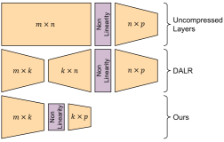
Figure 1: We propose a compression method with additional regularization terms for Domain Adaptation (DA) setting. Our method can maintain accuracy without fine-tuning after compression, and can achieve higher accuracy than prior work (DALR [Masana et al.(2017)Masana, van de Weijer, Herranz, Bagdanov, and Alvarez]). DALR is based on low-rank matrix decomposition, while our method is built on Spectral Pruning [Suzuki et al.(2020a)Suzuki, Abe, Murata, Horiuchi, Ito, Wachi, Hirai, Yukishima, and Nishimura].

In this work, we seek to adapt compression objectives to the specific setting of DA. Concretely, we are provided with both a source and a, possibly unlabeled, target distribution. We are interested in compressing DNNs with high accuracy on the target distribution. Some works have investigated this specific setting. The work in [Masana et al.(2017)Masana, van de Weijer, Herranz, Bagdanov, and Alvarez] is strongly related to ours but only focuses on the case where a model is fine-tuned on a target dataset. Their method yields great results in this setting because it is data-dependent. That is, compression depends on the input data distribution. In this paper, we focus on a compression method that is also data-dependent. The novelty of our work is to go further in the analysis of how the data affects compression and to add a new regularization term. This regularization term is directly related to a DA objective. It basically favors nodes that are non domain discriminative. This proves useful as the more similar the features extracted are, between source and target distribution, the more discriminative ability learned on the source distribution will also apply to the target distribution. Finally we show that our extended compression method compares favorably to [Masana et al.(2017)Masana, van de Weijer, Herranz, Bagdanov, and Alvarez] on various cases of fine-tuning a pre-trained model on a target dataset.

2 Related work

Here we present a brief review of the main strategies used in model compression. One can find in [Cheng et al.(2018)Cheng, Wang, Zhou, and Zhang] a more in-depth analysis of the different methods. (1) Pruning. These methods focus on finding weights of the network that are not crucial to the network’s performance. Early works used magnitude-based pruning which removed weights with the lowest values [Hanson and Pratt(1988)]. This method was extended by various works yielding significant results [Guo et al.(2016)Guo, Yao, and Chen, Li et al.(2018)Li, Qian, Jiang, Lu, and Tang]. In this work we focus on a pruning method [Suzuki et al.(2020a)Suzuki, Abe, Murata, Horiuchi, Ito, Wachi, Hirai, Yukishima, and Nishimura], which is based on spectral analysis of the covariance matrix of layers [Suzuki(2018), Suzuki et al.(2020b)Suzuki, Abe, and Nishimura]. (2) Network distillation. These approaches are based on a teacher-student learning scheme [Bucila et al.(2006)Bucila, Caruana, and Niculescu-Mizil, Ba and Caruana(2014), Hinton et al.(2015)Hinton, Vinyals, and Dean]. A compressed, small network will learn to mimic a large network or ensemble of large networks. This is efficient because the student model learns based on a combination of true labels, which are hard encoded, and soft outputs of the teacher model. Those contain valuable information about similarity between classes. Distillation can also train the student network to mimic the behavior of intermediate layers [Romero et al.(2015)Romero, Ballas, Kahou, Chassang, Gatta, and Bengio]. (3) Parameter quantization. Network quantization is based on finding an efficient representation of the network’s parameters by reducing the number of bits required to represent each weight. Various strategies can achieve this objective: [Gong et al.(2014)Gong, Liu, Yang, and Bourdev, Wu et al.(2016)Wu, Leng, Wang, Hu, and Cheng] applied k-means scalar quantization to the weight values. Other work use a fixed (8 or 16) bit representation of the weights while maintaining the accuracy of the original model [Vanhoucke et al.(2011)Vanhoucke, Senior, and Mao, Gupta et al.(2015)Gupta, Agrawal, Gopalakrishnan, and Narayanan]. In [Courbariaux et al.(2015)Courbariaux, Bengio, and David] a network is constrained to use only binary weights while still achieving high accuracy. (4) Low-rank factorization. The idea behind low-rank factorization and sparse techniques is to decompose layers into smaller ones with fewer parameters. For convolutional layers, main techniques rely on the fact that performing a convolution with the original filters can be approached by a linear combination of a set of convolutions with base filters [Sironi et al.(2015)Sironi, Tekin, Rigamonti, Lepetit, and Fua, Denton et al.(2014)Denton, Zaremba, Bruna, LeCun, and Fergus]. In [Masana et al.(2017)Masana, van de Weijer, Herranz, Bagdanov, and Alvarez] truncation of Singular Value Decomposition (SVD) is used to factorize the weight matrices of dense (fully connected) layers.

Some works explore pruning methods in DA (or transfer learning) setting [Molchanov et al.(2017)Molchanov, Tyree, Karras, Aila, and Kautz, Tung et al.(2017)Tung, Muralidharan, and Mori, Liu et al.(2017)Liu, Wang, and Qiao, Suau et al.(2020)Suau, Zappella, and Apostoloff, Zhong et al.(2018)Zhong, Li, Okada, and Maki, Yu et al.(2019)Yu, Wang, Chen, and Wu]. Unlike our work, most existing methods depend on iterative fine-tuning. Although each fine-tuning step may mitigate information loss caused by each pruning step, strong dependence on fine-tuning increases the risk of overfitting (see [Liu et al.(2019)Liu, Guo, and Chen] for more discussion).

In contrast to the iterative fine-tuning approach, the Domain Adaptive Low Rank Matrix Decomposition (DALR) method [Masana et al.(2017)Masana, van de Weijer, Herranz, Bagdanov, and Alvarez] can maintain accuracy without fine-tuning after compression. DALR and our method are data-dependent, which makes them suited for DA setting. Since DALR uses SVD, both are based on spectral analysis. An important difference between DALR and our method is their structural modification. We describe the difference, considering that uncompressed two layers have weight matrices of dimension $m\times n$ and $n\times p$ as shown in Fig. 1. For compressing the first layer, DALR produces two smaller layers that have weight matrices of dimension $m\times k$ and $k\times n$ ($k$ is kept rank). First, it is noted that, to actually reduce the number of parameters in the network, the parameter $k$ must verify the following condition: $k(m+n)<mn$. DALR affects only the layer being compressed since the output shape remains unchanged. Conversely, our method does not create additional layers but also affects the input dimension of the following layer. Second, DALR is only designed to compress dense layers while our method can be applied to both dense and convolutional layers. Finally, in [Masana et al.(2017)Masana, van de Weijer, Herranz, Bagdanov, and Alvarez], the authors only mention using $k$ as a given input to compression. Therefore compression and validation with various $k$ will be needed unless a prior knowledge of how much the layer is compressible is known. Our method helps to avoid this issue, using an information retention ratio parameter defined in Section 3.1. It should be noticed however that it is possible to reproduce a similar parametrization in DALR by computing the ratio of kept singular values over all singular values of the decomposition.

3 Spectral pruning with DA regularization

Our work was built on a layer-wise compression method [Suzuki et al.(2020a)Suzuki, Abe, Murata, Horiuchi, Ito, Wachi, Hirai, Yukishima, and Nishimura], which is based on spectral analysis. The method does not require any regularization during training, but is applicable to a pre-trained model. We will first detail this method then introduce our DA regularizer.

3.1 Principle

The method compresses the network layer per layer and can be applied to both dense and convolutional layers. It aims at reducing the dimension of the output of a layer such that the information of the input of the next layer remains mostly unchanged. To compress a layer, it selects the most informative nodes (neurons) or feature map channels (corresponding to convolutional filters). See Fig. 3 in [Han et al.(2015)Han, Pool, Tran, and Dally] and Fig. 2 in [He et al.(2017)He, Zhang, and Sun] for visual explanations of pruning dense and convolutional layers, respectively. For brevity, we will avoid the distinction of the layer types in the remainder of this paper and refer only to nodes for both cases.

More formally, let us denote $x$ the input to the network and suppose that we are given a training data $(x_{i},y_{i})_{i=1}^{n}$ with size $n$. Let us consider a model that is a sequence of convolutional and fully connected layers. We denote by $f^{l}$ and $\eta^{l}$ respectively the mapping function and activation function of a layer $l$. Finally we denote by $\phi^{l}(x)\in\mathbb{R}^{m_{l}}$ the representation obtained at layer $l$ where $m_{l}$ is the number of nodes in the layer $l$. Therefore we have $\phi^{l}(x)=\eta^{l}(f^{l}(\phi^{l-1}(x))).$ The objective of the method is to find for each layer $l$, the subset of nodes $J\subset\{1,\dots,m_{l}\}$ that minimizes the following quantity:

$$\hat{\mathrm{E}}[\|\phi^{l}(x)-\hat{A}_{J}\phi^{l}_{J}(x)\|^{2}],$$ (1)

where $\hat{\mathrm{E}}[.]$ denotes the empirical expectation, $\phi^{l}_{J}(x)$ denotes the vector composed of the components of $\phi^{l}(x)$ indexed by $J$, and $\hat{A}_{J}$ is a matrix to recover the whole vector $\phi^{l}$ from its sub-vector $\phi^{l}_{J}$ as well as possible.

For a fixed $J$, it is easy to minimize the objective (1) with respect to $\hat{A}_{J}$ as $\hat{A}_{J}=\hat{\Sigma}_{F,J}\hat{\Sigma}_{J,J}^{-1}$, where $\hat{\Sigma}:=\hat{\mathrm{E}}[\phi^{l}(x)\phi^{l}(x)^{\top}](=\frac{1}{n}\sum_{i=1}^{n}\phi^{l}(x_{i})\phi^{l}(x_{i})^{\top})$ is the empirical covariance matrix and $F:=\{1,\dots,m_{l}\}$ is the full set of indexes. Then $\phi^{l}(x)$ can be approximated by $\hat{A}_{J}\phi^{l}_{J}(x)$ which is equivalent to pruning the nodes of layer $l$ that do not belong to $J$ and reshaping the weights of the next layer. Let us denote $W_{l+1}$ the weight matrix if the next layer is a fully connected layer, $T_{l+1}$ the weight tensor if it is a convolutional layer. In that case we denote by the four dimensional tuple $(o_{c},i_{c},W,H)$ the shape of the weight tensor where $o_{c},i_{c},W,H$ stand respectively for output channels, input channels, width, height. The reshaping of the weights of the next layer is done the following way. For fully connected layers, we obtain the reshaped weight matrix as $\widetilde{W}^{l+1}=W^{l+1}\hat{A}_{J}.$ For convolutional layers, it is done by first reshaping $T_{l+1}$ to a $(W,H,o_{c},i_{c})$ tensor. Therefore each point of the filter grid is associated to a filter matrix $M_{w,h}\in\mathbb{R}^{o_{c}\times i_{c}}$ that will be reshaped by the operation: $\widetilde{M}_{w,h}=M_{w,h}\hat{A}_{J}.$ The tensor is then reshaped back to its original form $(o_{c},i_{c},W,H)$ where $i_{c}$ has been modified by the process.

Once we obtained the optimal $\hat{A}_{J}$ for a fixed $J$, then we minimize the objective (1) with respect to $J$. By substituting the optimal $\hat{A}_{J}$ to the objective function (1), it can be re-written as $\min_{J}\mathrm{Tr}[\hat{\Sigma}_{F,F}-\hat{\Sigma}_{F,J}\hat{\Sigma}_{J,J}^{-1}\hat{\Sigma}_{J,F}].$ The minimand in the right hand side is zero for $J=F$ and $\mathrm{Tr}[\hat{\Sigma}_{F,F}]$ for $J=\emptyset$. Hence we may consider the following “ratio” of residual as an information retention ratio $r$ to measure the relative goodness of $J$:

$$r=\frac{\mathrm{Tr}(\hat{\Sigma}_{F,J}\hat{\Sigma}_{J,J}^{-1}\hat{\Sigma}_{J,F})}{\mathrm{Tr}(\hat{\Sigma}_{F,F})}.$$ (2)

The higher the ratio the more information computed by the layer will be retained. It is no greater than 1 since the denominator is the best achievable value with no cardinality constraint. Compression can therefore be parametrized by a required information retention ratio parameter $\alpha$ and the final optimization problem translates to $\min_{J\subset F}|J|\ \ s.t.\ \ r\geq\alpha.$ To solve the optimization problem, the authors of [Suzuki et al.(2020a)Suzuki, Abe, Murata, Horiuchi, Ito, Wachi, Hirai, Yukishima, and Nishimura] proposed a greedy algorithm where $J$ is constructed by sequentially adding the node that maximizes the information retention ratio.

It is worth noticing that though the method is aimed at compressing each layer sequentially, using $\alpha$ allows more flexibility than methods with a fixed compression rate for each layer. Since we do not impose constraints on the cardinality of $J$, compression will adapt to the inherent compressibility of the layer. We argue that this makes $\alpha$ an easy to tune and intuitive hyperparameter and, if necessary, can easily be combined with cardinality constraints.

3.2 Domain Adaptation regularization

In DA setting, informative nodes could be different between source and target domains. To adjust this difference, we propose an additional regularization term to select better nodes.

As shown by [Ben-David et al.(2010)Ben-David, Blitzer, Crammer, Kulesza, Pereira, and Vaughan], one of the main challenges of DA is to find a representation discriminative with respect to the classification task but not discriminative between domains. The general idea is that, by matching the two distributions, the classification knowledge learned on the labeled source data can be transferred to the target data. Therefore, we propose to use a measure of the alignment of the source and target features distributions for selecting nodes during compression. We call our method Moment Matching Spectral Pruning (MoMaSP).

Previous work involving covariance alignment achieved high accuracy in DA tasks [Sun et al.(2016)Sun, Feng, and Saenko]. Following those observations, we define our regularization term as the following

$$\begin{split}R_{J}=\|\hat{\mathrm{E}}_{x\sim X^{s}}[\phi^{l}_{J}(x)]-\hat{\mathrm{E}}_{x\sim X^{t}}[\phi^{l}_{J}(x)]\|+\|S_{J,J}\odot(C^{s}_{J,J}-C^{t}_{J,J})\|_{\mathrm{F}},\end{split}$$ (3)

where $X^{s},X^{t}$ denotes the source and target distributions, $C^{s},C^{t}$ respectively the source and target empirical covariance matrices, $S$ a scaling matrix defined by $S_{ij}=(C^{t}_{i,i}C^{t}_{j,j})^{-\frac{1}{4}}$, $\odot$ denotes the element wise multiplication, and $\|\cdot\|_{\mathrm{F}}$ means the Frobenius norm of a matrix. This quantity measures the discrepancy between the source and target distributions by using the up-to second order statistics. The first term measures the discrepancy of mean and the second term measures the discrepancy of the (scaled) second order moment. Hence, this regularization term induces a moment matching effect and the two distributions become similar on the selected nodes. We may use the MMD criterion (kernel-based discrepancy measure) [Gretton et al.(2012)Gretton, Borgwardt, Rasch, Schölkopf, and Smola] to capture not only the first and second moments but also all higher moments instead, but we found that it takes too much computational time. Although the kernelized alignment loss [Koniusz et al.(2017)Koniusz, Tas, and Porikli] could speed-up computation, source and target samples per class need to be few.

Instead of the criterion (3), we also consider the following alternative formulation:

$$\begin{split}R_{j}=\|\hat{\mathrm{E}}_{x\sim X^{s}}[\phi^{l}_{j}(x)]-\hat{\mathrm{E}}_{x\sim X^{t}}[\phi^{l}_{j}(x)]\|+\|S_{j,F}\odot(C^{s}_{j,F}-C^{t}_{j,F})\|.\end{split}$$ (4)

The first formulation (3) depends on the whole subset $J$ while the second one computes information more specific to each node. The second formulation is more computationally efficient since the $R_{j}$’s can be computed only once for each candidate index. The first one needs to recompute it for every candidate index at each step of the procedure because of its dependence on $J$.

3.3 Intuition behind our regularization

The intuition behind our regularization is the following. In DA setting where few or no labels are available on the target distribution, the discriminative knowledge is learned mainly on the source distribution. Thus the feature distributions on both domains should be aligned for the discriminative knowledge learned on the source domain to apply to the target domain. When comparing the information retention ratios of Eq. 2 for different nodes, we observed that many of them had very close values. This means that many nodes capture approximately the same amount of information, in the sense of total variance. Our intuition was that when these relative differences are too small, they are not significant to discriminate between nodes and are more likely the result of noise. Therefore a better criterion should be used to differentiate nodes that capture a same amount of variance. Since our compression method is designed to be applied on models that have been trained using DA methods, it is natural to use a criterion related to DA objectives. We choose to compare nodes based on how well their feature distributions on source and target domains are aligned. Nodes leading to a better alignment should be favored as they will allow for a better transfer of discriminative knowledge from source to target domain. Our method realizes this via a moment matching type regularization.

3.4 Practical implementation

We present in Algorithm 1 a pseudo code for a practical implementation of our method using the first formulation of our regularizer. If the second formulation is used, the regularization term for each node is computed only once before entering the while loop as it does not depend on $J$. At each step of the algorithm, we denote by $C$ the set of candidate indexes. To select which node to add to $J$, the ratio from Eq. (2) is computed for each candidate index. We denote by $V$ the vector where each coordinate corresponds to the ratio value of a candidate index. Similarly, we denote by $R_{J}$ the vector where each coordinate correspond to the regularizing term associated to a candidate index.

Without regularization, the index to add to $J$ is

Input : $\hat{\Sigma}_{F,F}$ : Empirical covariance matrix,

$\alpha$ : Required information retention ratio

Output : $J$ : Subset of selected nodes

Function FindSubset$(\hat{\Sigma}_{F,F},\alpha)$

      

      $J\leftarrow\emptyset$

       $T\leftarrow\mathrm{Tr}(\hat{\Sigma}_{F,F})$

       $r\leftarrow 0$

       $C\leftarrow F$

       while $r<\alpha$ do

             for $j\in C$ do

                   $J_{j}\leftarrow J\cup j$

                   Compute $R_{J_{j}}$

                   $V_{j}\leftarrow\frac{\mathrm{Tr}(\hat{\Sigma}_{F,J_{j}}\hat{\Sigma}_{J_{j},J_{j}}^{-1}\hat{\Sigma}_{J_{j},F})}{T}$

             end for

            $i\leftarrow\underset{j\in C}{\operatorname{arg\,max}}\left\{V_{j}-\lambda\cdot\mathrm{\sigma}(V)\cdot\frac{R_{J_{j}}}{\max_{j^{\prime}}(R_{J_{j^{\prime}}})}\right\}$

             $J\leftarrow J\cup\{i\}$

             $r\leftarrow V_{i}$

             $C\leftarrow C\setminus\{i\}$

       end while

      

end

Algorithm 1 MoMaSP

simply given by $i=\mathop{\mathrm{arg\,max}}_{j\in C}V_{j}.$ Using regularization, the index to add to $J$ is chosen as

$$i=\mathop{\mathrm{arg\,max}}_{j\in C}\left\{V_{j}-\lambda\cdot\mathrm{\sigma}(V)\cdot\frac{R_{J_{j}}}{\max_{j^{\prime}}(R_{J_{j^{\prime}}})}\right\},$$ (5)

where $\sigma(V)$ is the standard deviation of $(V_{j})_{j\in C}$. The values of $R_{J_{j}}$ are rescaled to be in the same range as $V_{j}$’s by max normalization. Multiplying by $V$’s standard deviation, $\sigma(V)$, ensures that the regularization will be applied at the right scale. It should only slightly modify the relative ordering of the values in $V$ as the main criteria for selection must remain the information ratio. Indeed, only taking into account the regularization term would favor nodes that output a constant value across both distributions. The hyperparameter $\lambda$ allows for more control over the trade-off between those two terms. We use $1$ as the default $\lambda$ in our experiments. The max normalization and scaling make $\lambda$ easier to tune. This compression is applied after training and can therefore be combined with any DA method.

4 Experiments on digits images

In this section, we conduct experiments with a model trained on digits datasets, using a DA technique [Saito et al.(2018)Saito, Watanabe, Ushiku, and Harada]. The source dataset is the SVHN dataset [Netzer et al.(2011)Netzer, Wang, Coates, Bissacco, Wu, and Ng] and the target dataset is the MNIST dataset [LeCun et al.(1998)LeCun, Bottou, Bengio, and Haffner], which are standard for DA with adversarial training [Ganin et al.(2016)Ganin, Ustinova, Ajakan, Germain, Larochelle, Laviolette, March, and Lempitsky, Saito et al.(2018)Saito, Watanabe, Ushiku, and Harada, Tzeng et al.(2017)Tzeng, Hoffman, Saenko, and Darrell].

4.1 Model

Considering the relative simplicity of the task, we used a custom model composed of a 4 layers feature generator (3 convolutional + 1 dense) and a 2 layers classifier (see Supplementary Material for details). To train the model we used the DA technique presented in [Saito et al.(2018)Saito, Watanabe, Ushiku, and Harada] which utilizes “maximum classifier discrepancy." Briefly, the adaptation is realized by adversarial training of a feature generator network and two classifier networks. The adversarial training forces the feature generator to align the source and target distribution. Contrary to other methods relying on adversarial training with a domain discriminator, this method considers the decision boundary while aligning the distributions, ensuring that the generated features are discriminative with respect to the classification task at hand.

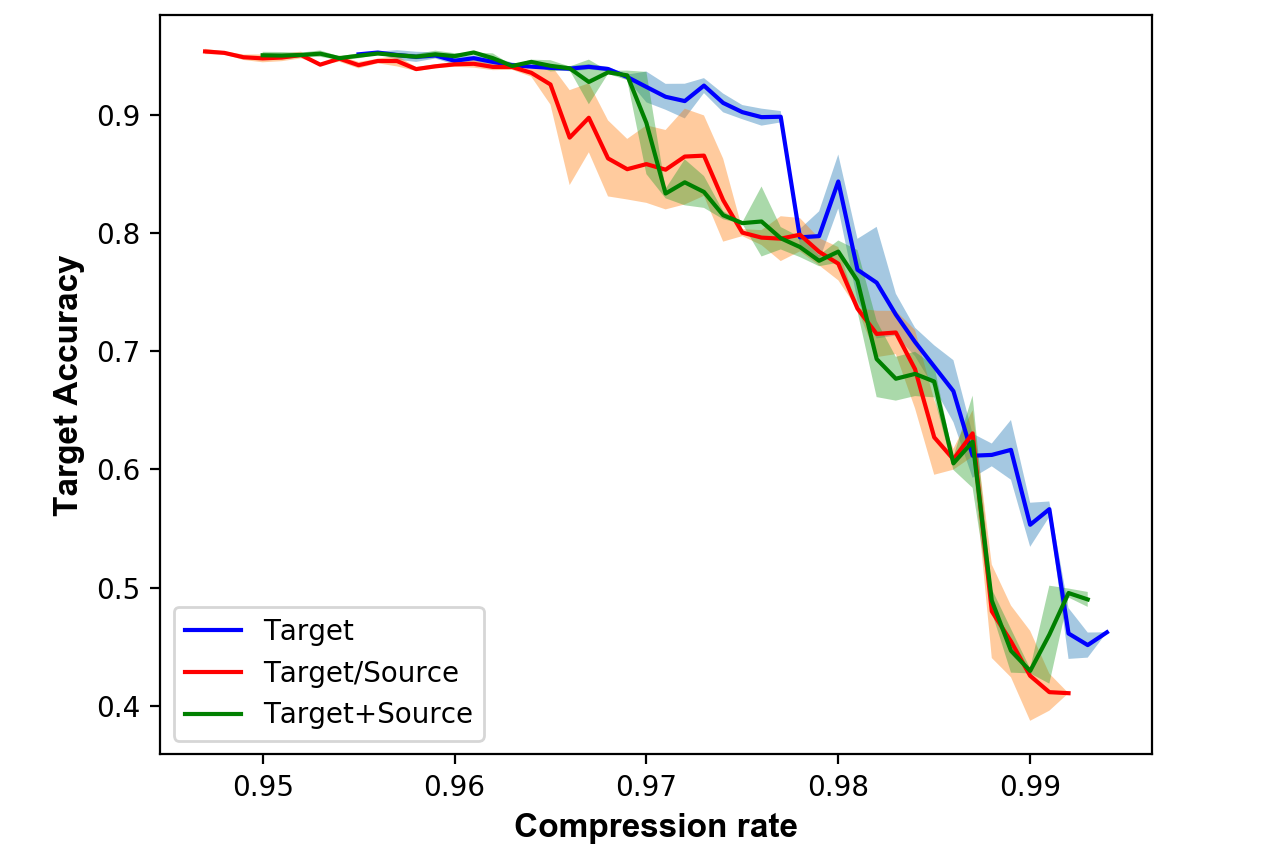
Figure 2: Target accuracy over compression rate for three different settings of data used as input. Results are presented as mean +/- standard deviation based on 10 iterations.

Test data	First layer nodes specificity
	Source	Target	None
Source	0.79	0.77	0.72
Target	0.65	0.84	0.71

Table 1: Mean activation rates.

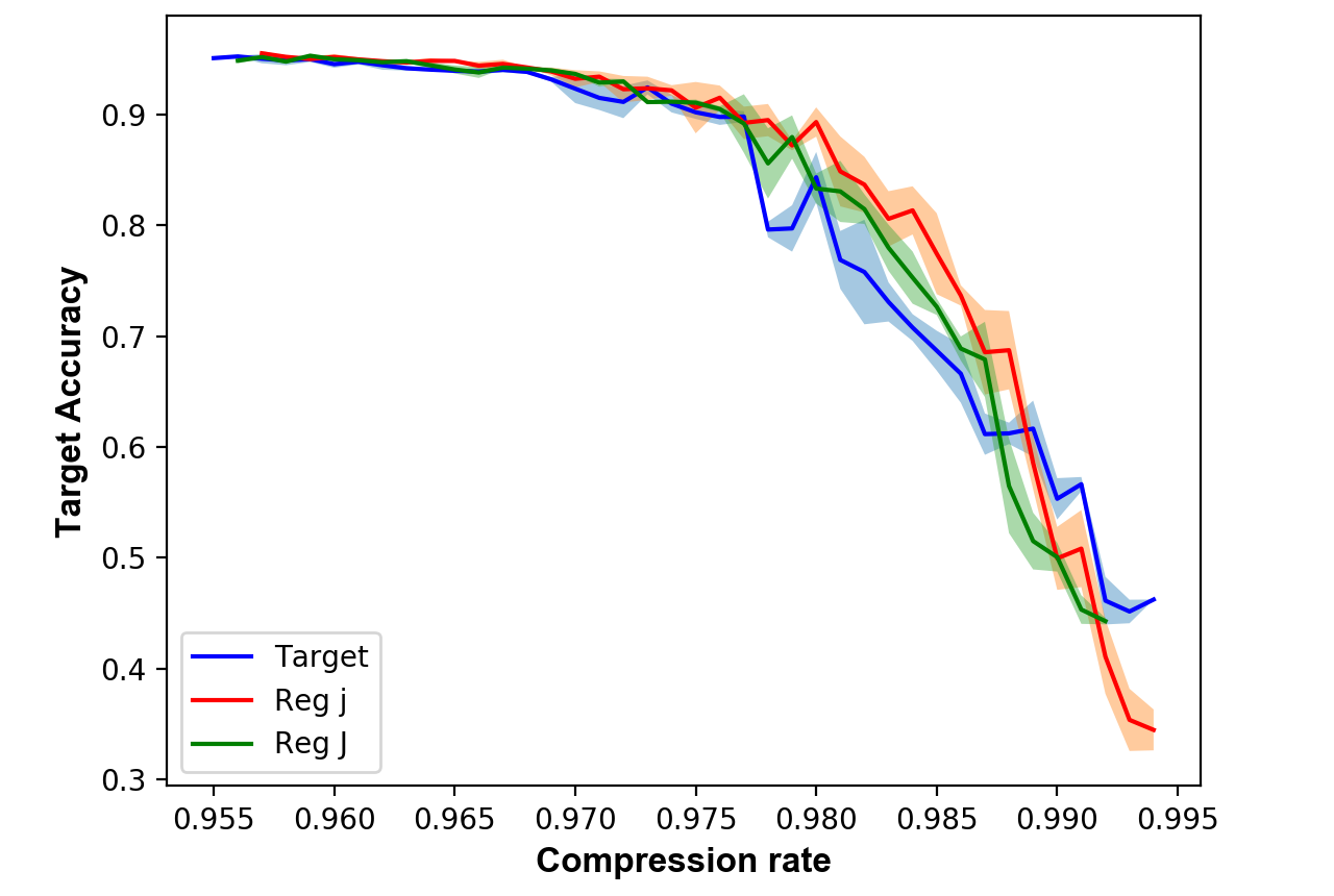
Figure 3: Comparison using only target data or each formulation of our DA regularization. Results are presented as mean +/- standard deviation based on 10 iterations.

C.R. (%)	96.0	96.5	97.0	97.5	98.0	98.5
Target (%)	94.6	94.0	92.4	90.2	84.4	68.7
Reg $J$ (%)	95.0	94.1	93.7	91.1	83.3	72.7
Reg $j$ (%)	95.2	94.9	94.3	90.6	89.3	77.5

Table 2: Accuracy on target test dataset for different compression rate (C.R.).

4.2 Data choice for compression

The uncompressed model was trained using both train splits and evaluated on the test split of MNIST. It reached an accuracy of 96.64%, similar to the results obtained in the original paper [Saito et al.(2018)Saito, Watanabe, Ushiku, and Harada]. We then apply compression on the trained model. During compression, only data of the train splits was used and the compressed models were evaluated on the MNIST test split. Since the method is data-dependent, the choice of data to use to compute the empirical covariance matrix should be taken care of. Three different settings were tested: (1) Target: Using 14,000 samples from the target distribution; (2) Target/Source: Using 7,000 samples from the target distribution and 7,000 samples from the source distribution; and (3) Target+Source: Using 14,000 samples from the target distribution and 7,000 additional samples from the source distribution. The results obtained are presented in Fig. 2. Using only target samples to compute the covariance matrix shows the best performance.

To give a better understanding of this result, we conducted an analysis about how the nodes activation pattern depends on data distribution as follows: we compressed the first layer of a trained network using either only target data or only source data. We then compared the activation of nodes that were selected only in one of the two cases, in other words, nodes specific to target or source data. We show the results in Table 1.

As expected, nodes selected using source data had a significantly higher activation rate on the source distribution and conversely for target specific nodes. As a control case, we added activation of nodes that were selected in neither of the two settings. Those do not show any significant difference in their activation. Interestingly, this difference was no longer appearing when comparing activation of the last fully connected layer, because DA training aligns the distributions of extracted features. This experiment sheds light on how the input data affects the compression of data-dependent methods. In case of a model trained on different distributions with DA, early layers contain nodes that are specific to each distribution. Thus it is critical for compression to use data coming exclusively from the distribution the model will be applied to. Partially using source data forces compression in the early layers to select source specific nodes to the expense of target specific nodes leading to poorer results.

4.3 Regularization for compression

Finally we compared the results of the best baseline, using only target data, with adding the regularization term introduced in Section 3. The results are presented in Fig. 3 and summarized in Table 2. It appears that the second formulation of our regularizer gives the best performance. This is probably due to the fact it focuses on node level information and not on the whole subset $J$, giving better ability to discriminate against specific nodes.

Compared to the baseline, our regularizer leads to significant improvements in compression performance. We observe up to 9% bumps in accuracy. Yet, we notice that the baseline performs slightly better for very high compression rates. We conjecture that reducing information loss becomes more important for such compression rates and our regularization with $\lambda{=}1$ is too strong. There is room for improvement by tuning the hyperparameter $\lambda$ depending on the compression rate or developing methods for adaptive regularization.

5 Experiments on natural images

In this section, we compare our method (MoMaSP) with the factorization based compression method (DALR) in [Masana et al.(2017)Masana, van de Weijer, Herranz, Bagdanov, and Alvarez]. We reproduce the same setting as in their experiment: a VGG19 model pre-trained on the ImageNet dataset [Russakovsky et al.(2015)Russakovsky, Deng, Su, Krause, Satheesh, Ma, Huang, Karpathy, Khosla, Bernstein, Berg, and Fei-Fei] is fine-tuned on different target datasets.

5.1 Experimental settings

We establish our comparison based on the following three datasets used in [Masana et al.(2017)Masana, van de Weijer, Herranz, Bagdanov, and Alvarez] experiments: Oxford 102 Flowers [Nilsback and Zisserman(2008)], CUB-200-2011 Birds [Wah et al.(2011)Wah, Branson, Welinder, Perona, and Belongie], and Stanford 40 Actions [Yao et al.(2011)Yao, Jiang, Khosla, Lin, Guibas, and Fei-Fei].

For all three datasets, we first trained uncompressed models by fine-tuning from an ImageNet pre-trained VGG19 model. In the fine-tuning before compression, we trained the weights of the fully connected layers while keeping the weights of the convolutional layers frozen to their pre-trained value on ImageNet like [Masana et al.(2017)Masana, van de Weijer, Herranz, Bagdanov, and Alvarez].

We then compressed the models. The input data to compression was always composed of 4,000 samples of the train split, except for the Oxford 102 Flowers where the whole train split was used. Additional 4,000 randomly sampled images from the ImageNet train split were used for DA regularization. Note that our method and DALR [Masana et al.(2017)Masana, van de Weijer, Herranz, Bagdanov, and Alvarez] do not need the labels of target datasets in this compression phase. After that we optionally fine-tuned the fully connected layers of compressed models with target labels.

We used the Adam optimizer [Kingma and Ba(2015)] with a batch size of 50, a learning rate of $10^{-4}$, and a weight decay of $5{\times}10^{-4}$ for training models. See Supplementary Material for details.

5.2 VGG19 fc7 compression

We first evaluated the compression on the last fully connected layer (fc7) of the model, containing 4,096 nodes, because the fc7 compression is a main evaluation setting in [Masana et al.(2017)Masana, van de Weijer, Herranz, Bagdanov, and Alvarez]. For each trial we report the results both with and without fine-tuning of the classifier layers after compression. We also report the results of compression using basic SVD on fc7 weight matrix as a baseline to further illustrate the advantage of using data-dependent methods. To compare our method with DALR, a dimension $k$ was set for the compression using DALR then $k^{\prime}$, the dimension to keep in our method resulting in an equal number of parameters, was determined accordingly. See Supplementary Material for details.

The results are presented in Tables 4, 4, and 6. We show the relative numbers of parameters in the fc7 layer compressed by DALR in the “params” rows in the tables as in the DARL paper [Masana et al.(2017)Masana, van de Weijer, Herranz, Bagdanov, and Alvarez]. In all experiments, our method maintains high accuracy even for high compression rates. In such cases it outperforms DALR by a large margin. However, for lower compression rates DALR consistently compares favorably to our method though the difference is arguably small. In most cases, fine-tuning does not improve much the performance of any of the two methods, except for DALR for high compression rates. This phenomenon implies that the learning rate and/or the dropout rate we used are too high especially for our method (see additional fine-tuning results in Supplementary Material for details).

$k$	$4$	$8$	$16$	$32$	$64$	$128$
params (%)	0.20	0.39	0.78	1.56	3.13	6.25
SVD w/o FT.	5.2	12.8	30.2	54.6	65.2	67.6
SVD w/ FT.	13.7	36.7	56.6	65.9	70.0	70.8
DALR w/o FT.	8.6	31.1	55.1	66.9	71.0	72.8
DALR w/ FT.	18.9	48.2	64.4	70.3	70.7	72.3
Ours w/o FT.	68.9	69.3	70.0	71.2	72.0	72.5
Ours w/ FT.	67.3	68.9	70.3	69.9	70.8	70.6

Table 3: VGG19 fc7 compression on Oxford 102 Flowers. Test dataset accuracy results (%). Original accuracy: 73.1%.

$k$	$4$	$8$	$16$	$32$	$64$	$128$
params (%)	0.20	0.39	0.78	1.56	3.13	6.25
SVD w/o FT.	4.1	12.6	30.3	46.9	54.8	60.5
SVD w/ FT.	17.3	39.1	51.2	57.2	58.8	58.5
DALR w/o FT.	5.6	23.1	49.3	57.8	60.1	60.9
DALR w/ FT.	19.0	40.9	54.0	59.8	59.3	59.5
Ours w/o FT.	58.3	58.2	58.2	58.8	59.3	60.2
Ours w/ FT.	57.9	57.3	57.7	58.2	58.2	59.7

Table 4: VGG19 fc7 compression on CUB-200-2011 Birds. Test dataset accuracy results (%). Original accuracy: 61.5%.

$k$	$4$	$8$	$16$	$32$	$64$	$128$
params (%)	0.20	0.39	0.78	1.56	3.13	6.25
SVD w/o FT.	17.1	31.0	54.5	67.3	72.2	72.7
SVD w/ FT.	45.4	62.0	68.6	72.8	73.1	73.7
DALR w/o FT.	20.7	43.3	65.0	73.0	74.3	74.7
DALR w/ FT.	46.8	63.3	69.6	73.5	72.9	72.9
Ours w/o FT.	69.0	70.2	71.8	73.1	73.9	73.8
Ours w/ FT.	70.5	70.4	71.7	72.9	73.7	74.0

Table 5: VGG19 fc7 compression on Stanford 40 Actions. Test dataset accuracy results (%). Original accuracy: 74.6%.

	Layers		FT.	C.R. (%)	#params	Accuracy (%)
	conv	fc				Oxford	CUB	Stanford
DALR		✓		84.9	21.1 M	48.1	43.0	57.7
		✓	✓			62.2	52.8	67.4
Ours		✓		85.0	21.1 M	48.1	37.1	61.0
		✓	✓			63.9	55.1	69.0
Ours	✓	✓		85.4	20.4 M	60.6	51.4	69.2
	✓	✓	✓			71.4	58.3	72.6

Table 6: VGG19 full compression on each dataset.

5.3 VGG19 full compression

It is important to notice that, contrary to DALR, our method is able to compress both convolutional and dense layers. To further demonstrate this advantage, we proceeded to the comparison of fully compressing the VGG19 network using both methods. We conducted the experiment on all three datasets. DALR was applied to the fully connected layers. The dropout layers of models compressed by our method were disabled in fine-tuning, because our method reduce the input dimension of the dropout layers unlike DALR, resulting in performance degradation. See Supplementary Material for other details.

Results are presented in Table 6. For all three datasets, our method consistently achieves a better compression rate (C.R.) while reaching test accuracy 5.2%–12.5% higher than DALR. If we apply our method to the fully connected layers only, the difference in accuracy is smaller but still favorable to our method in many cases. Although further improvement would be preferable to keep representations for many classes (CUB-200 without fine-tuning), in practice, it is not necessary to overcompress the fully connected layers by our method.

5.4 Discussion

Our method is drastically better for high compression rates, while DALR is slightly better for low compression rates. We conjecture that this is mainly due to the fact that the two methods modify differently the network (see Fig. 1). DALR affects only one layer. Therefore if the compression is too important, it reaches a critical point where not enough information can possibly be retained. Our method affects two successive layers therefore spreading the effect of compression and avoiding this critical point for high compression rates. On the other hand, our method needs to consider nonlinearity between two layers and uses a greedy algorithm [Suzuki et al.(2020a)Suzuki, Abe, Murata, Horiuchi, Ito, Wachi, Hirai, Yukishima, and Nishimura]. Thus only affecting one layer is better to maintain high accuracy for lower compression rates, because the output of the one layer can be optimally approximated.

The optimization problem to solve in DALR admits a closed form solution, making it a very fast compression method. Compared to DALR, it is a limitation of our method to require an iterative optimization. However, the extra computational time is usually a few hours on 1 GPU (Tesla V100) in our experiments. Furthermore, an iterative process is used in the DALR paper [Masana et al.(2017)Masana, van de Weijer, Herranz, Bagdanov, and Alvarez] to determine compression rate pairs for fc6 and fc7, and it needs iterative accuracy evaluation. Pruning methods based on iterative fine-tuning approach also take time for pruning, fine-tuning, and evaluation. Therefore our method is practical enough.

6 Conclusions

In this paper, we investigated compression of DNNs in the DA setting. As shown by [Masana et al.(2017)Masana, van de Weijer, Herranz, Bagdanov, and Alvarez], using a data-dependent method is crucial in order to achieve good results. In that matter, our work shows that the input data to calculate information retention ratio for compression should only come from the distribution on which the model will be applied to, the target distribution in our case. This is because adding samples from another distribution will force compression in the early layers to select nodes that are specific to this distribution. However, we show that source data can still be used for regularization to improve nodes selection. This is done by comparing the first and second order statistics of the node’s feature distributions on each of the source and target data. This criterion serves as a measure of the alignment of the two distributions which directly relates to DA objectives. Therefore we denote this measure as a DA regularizer. We evaluated this regularization on a spectral pruning method introduced in [Suzuki et al.(2020a)Suzuki, Abe, Murata, Horiuchi, Ito, Wachi, Hirai, Yukishima, and Nishimura] and obtained significant improvements on its compression results. Finally we compared our regularized compression method with the factorization based method of [Masana et al.(2017)Masana, van de Weijer, Herranz, Bagdanov, and Alvarez] on real world image datasets. Our method compares favorably on all three datasets, leading to significant improvements in retained accuracy for high compression rates.

Although our work focused on one compression method, we argue that using first and second order statistics of feature distributions to measure the alignment between source and target features and using it as a criterion for compression can be applied to other methods. This work can therefore serve as a first example and practical implementation of this idea. Applying our method to unsupervised DA setting [Yu et al.(2019)Yu, Wang, Chen, and Wu, Koniusz et al.(2018)Koniusz, Tas, Zhang, Harandi, Porikli, and Zhang] is an interesting future direction.

Acknowledgements

TS was partially supported by JSPS KAKENHI (26280009, 15H05707, and 18H03201), Japan Digital Design, and JST-CREST.

Supplementary Material

Appendix A Experimental settings on digits images

The output widths of the layers of the custom model are $(64,64,128,1024,1024,10)$. Each convolutional or dense layer except for the output layer is followed by a batch normalization layer and a ReLU layer, and the feature generator is followed by a dropout layer.

Appendix B Experimental settings on natural images

We establish our comparison based on three datasets used in [Masana et al.(2017)Masana, van de Weijer, Herranz, Bagdanov, and Alvarez] experiments.

• Oxford 102 Flowers [Nilsback and Zisserman(2008)]: contains 8,189 images. Train and validation splits contain each 1,020 samples with each class equally represented. Test split contains 6,149 samples with classes not equally represented.
  

• CUB-200-2011 Birds [Wah et al.(2011)Wah, Branson, Welinder, Perona, and Belongie]: contains 11,788 images (5,994 train, 5,794 test) of 200 bird species. Although each image is annotated with bounding box, part location (head and body), and attribute labels, those annotations were not used in our experiments.
  

• Stanford 40 Actions [Yao et al.(2011)Yao, Jiang, Khosla, Lin, Guibas, and Fei-Fei]: contains 9,532 images (4,000 train, 5,532 test) of 40 categories corresponding to different human actions. Classes are equally represented on the training set and all samples contain at least one human performing the corresponding action.

We used an ImageNet pre-trained VGG19 model that provided by the torchvision package of PyTorch. We trained for 10 epochs on Oxford-102 Flowers, 5 epochs on CUB-200 Birds, and 5 epochs on Stanford 40 Actions for fine-tuning before compression. On each dataset, we trained five models to mitigate randomness, and used the model that has the median accuracy of the five models as the original (uncompressed) model. When we fine-tune models after compression, we trained for 2 epochs and 5 epochs for VGG19 fc7 compression and VGG19 full compression, respectively. The dropout rate of VGG19 was set to 0.5. All models were trained using PyTorch.

In the case of VGG19 fc7 compression, compression rates for the total parameters of VGG19 models are limited to 11%–12% and FLOPs reduction is negligible, because layers before the fc7 layer are not compressed.

To compare our method with DALR, we need a way to fit the numbers of parameters because the two methods do not modify the architecture of the network the same way. DALR replaces a fully connected layer by two smaller layers without changing the next layer. Our method keeps the same number of layers but also affects the input dimension of the next layer. Therefore we proceeded the following way to compare the two methods objectively. A dimension $k$ was set for the compression using DALR then $k^{\prime}$, the dimension to keep in our method resulting in an equal number of parameters, was determined accordingly. More precisely, the fc7 layer has a weight matrix of dimension $m\times m$ (because $m$ and $n$ in Fig. 1 are the same value for the fc7 layer) and the next layer has a weight matrix of dimension $m\times p$. Taking into account the biases we get the following equation:

$$k^{\prime} =\frac{m(2k+1+p)+k}{m+1+p}.$$ (6)

The iterative process of the DALR paper [Masana et al.(2017)Masana, van de Weijer, Herranz, Bagdanov, and Alvarez] for determining compression rate for each layer is computationally inefficient. Thus, for VGG19 full compression, we did not determine compression rate for each layer automatically for both methods. Specifically, for compression by DALR, compression rate for fc8 is set to 0.5 (a modest value for not breaking output values), and compression rate for other layers (fc6 and fc7) is set so that total compression rate becomes $\sim$85%. For our method, compression rate for fully connected layers is set to 0.96, and compression rate for convolutional layers is set so that total compression rate becomes over 85%. Although the FLOPs reduction by DALR is negligibly small, our method reduces FLOPs by $\sim$19% thanks to the compression of convolutional layers.

Appendix C Fine-tuning results on natural images

In many cases, fine-tuning degrades the performance of our method. To investigate this phenomenon, we evaluated other models that fine-tuned for various epochs on Oxford 102 Flowers. The results are presented in Table 7. The accuracy drops in the first epoch and recovers in succeeding epochs. Considering these results, the learning rate and/or the dropout rate we used are too high for our method, and they cause the performance drops by keeping parameters away from optimal values. Tuning learning rates, dropout rates, and epochs for fine-tuning by cross-validation will further improve accuracy, though it takes much time.

$k$	$4$	$8$	$16$	$32$	$64$	$128$
Ours w/o FT.	68.9	69.3	70.0	71.2	72.0	72.5
Ours 1 epoch FT.	64.0	63.9	64.9	67.7	69.5	67.8
Ours 2 epochs FT.	67.3	68.9	70.3	69.9	70.8	70.6
Ours 5 epochs FT.	71.9	72.9	73.2	73.5	74.2	74.2

Table 7: Accuracy transition by fine-tuning. VGG19 fc7 compression on Oxford 102 Flowers. Test dataset accuracy results (%).

References

- [Ba and Caruana(2014)] Jimmy Ba and Rich Caruana. Do deep nets really need to be deep? In NIPS. 2014.
- [Ben-David et al.(2010)Ben-David, Blitzer, Crammer, Kulesza, Pereira, and Vaughan] Shai Ben-David, John Blitzer, Koby Crammer, Alex Kulesza, Fernando Pereira, and Jennifer Wortman Vaughan. A theory of learning from different domains. Machine Learning, 2010.
- [Bucila et al.(2006)Bucila, Caruana, and Niculescu-Mizil] Cristian Bucila, Rich Caruana, and Alexandru Niculescu-Mizil. Model compression. In KDD, 2006.
- [Cheng et al.(2018)Cheng, Wang, Zhou, and Zhang] Yu Cheng, Duo Wang, Pan Zhou, and Tao Zhang. Model compression and acceleration for deep neural networks: The principles, progress, and challenges. IEEE Signal Processing Magazine, 2018.
- [Courbariaux et al.(2015)Courbariaux, Bengio, and David] Matthieu Courbariaux, Yoshua Bengio, and Jean-Pierre David. BinaryConnect: Training deep neural networks with binary weights during propagations. In NIPS, 2015.
- [Denton et al.(2014)Denton, Zaremba, Bruna, LeCun, and Fergus] Emily Denton, Wojciech Zaremba, Joan Bruna, Yann LeCun, and Rob Fergus. Exploiting linear structure within convolutional networks for efficient evaluation. In NIPS. 2014.
- [Ganin et al.(2016)Ganin, Ustinova, Ajakan, Germain, Larochelle, Laviolette, March, and Lempitsky] Yaroslav Ganin, Evgeniya Ustinova, Hana Ajakan, Pascal Germain, Hugo Larochelle, François Laviolette, Mario March, and Victor Lempitsky. Domain-adversarial training of neural networks. JMLR, 2016.
- [Gong et al.(2014)Gong, Liu, Yang, and Bourdev] Yunchao Gong, Liu Liu, Ming Yang, and Lubomir D. Bourdev. Compressing deep convolutional networks using vector quantization. arXiv:1412.6115, 2014.
- [Gretton et al.(2012)Gretton, Borgwardt, Rasch, Schölkopf, and Smola] Arthur Gretton, Karsten M. Borgwardt, Malte J. Rasch, Bernhard Schölkopf, and Alexander Smola. A kernel two-sample test. JMLR, 2012.
- [Guo et al.(2016)Guo, Yao, and Chen] Yiwen Guo, Anbang Yao, and Yurong Chen. Dynamic network surgery for efficient dnns. In NIPS. 2016.
- [Gupta et al.(2015)Gupta, Agrawal, Gopalakrishnan, and Narayanan] Suyog Gupta, Ankur Agrawal, Kailash Gopalakrishnan, and Pritish Narayanan. Deep learning with limited numerical precision. In ICML, 2015.
- [Han et al.(2015)Han, Pool, Tran, and Dally] Song Han, Jeff Pool, John Tran, and William Dally. Learning both weights and connections for efficient neural network. In NIPS. 2015.
- [Hanson and Pratt(1988)] Stephen Jose Hanson and Lorien Y. Pratt. Comparing biases for minimal network construction with back-propagation. In NIPS. 1988.
- [He et al.(2016)He, Zhang, Ren, and Sun] Kaiming He, Xiangyu Zhang, Shaoqing Ren, and Jian Sun. Deep residual learning for image recognition. In CVPR, 2016.
- [He et al.(2017)He, Zhang, and Sun] Yihui He, Xiangyu Zhang, and Jian Sun. Channel pruning for accelerating very deep neural networks. In ICCV, 2017.
- [Hinton et al.(2015)Hinton, Vinyals, and Dean] Geoffrey E. Hinton, Oriol Vinyals, and Jeff Dean. Distilling the knowledge in a neural network. arXiv:1503.02531, 2015.
- [Jaderberg et al.(2014)Jaderberg, Vedaldi, and Zisserman] Max Jaderberg, Andrea Vedaldi, and Andrew Zisserman. Speeding up convolutional neural networks with low rank expansions. In BMVC, 2014.
- [Kingma and Ba(2015)] Diederik Kingma and Jimmy Ba. Adam: A method for stochastic optimization. In ICLR, 2015.
- [Koniusz et al.(2017)Koniusz, Tas, and Porikli] Piotr Koniusz, Yusuf Tas, and Fatih Porikli. Domain adaptation by mixture of alignments of second- or higher-order scatter tensors. In CVPR, 2017.
- [Koniusz et al.(2018)Koniusz, Tas, Zhang, Harandi, Porikli, and Zhang] Piotr Koniusz, Yusuf Tas, Hongguang Zhang, Mehrtash Harandi, Fatih Porikli, and Rui Zhang. Museum exhibit identification challenge for the supervised domain adaptation and beyond. In ECCV, 2018.
- [Krizhevsky et al.(2012)Krizhevsky, Sutskever, and Hinton] Alex Krizhevsky, Ilya Sutskever, and Geoffrey E. Hinton. ImageNet classification with deep convolutional neural networks. In NIPS. 2012.
- [LeCun et al.(1998)LeCun, Bottou, Bengio, and Haffner] Yann LeCun, Léon Bottou, Yoshua Bengio, and Patrick Haffner. Gradient-based learning applied to document recognition. Proceedings of the IEEE, 1998.
- [Li et al.(2018)Li, Qian, Jiang, Lu, and Tang] Guiying Li, Chao Qian, Chunhui Jiang, Xiaofen Lu, and Ke Tang. Optimization based layer-wise magnitude-based pruning for DNN compression. In IJCAI, 2018.
- [Liu et al.(2019)Liu, Guo, and Chen] Bingyan Liu, Yao Guo, and Xiangqun Chen. WealthAdapt: A general network adaptation framework for small data tasks. In ACMMM, 2019.
- [Liu et al.(2017)Liu, Wang, and Qiao] Jiaming Liu, Yali Wang, and Yu Qiao. Sparse deep transfer learning for convolutional neural network. In AAAI, 2017.
- [Masana et al.(2017)Masana, van de Weijer, Herranz, Bagdanov, and Alvarez] Marc Masana, Joost van de Weijer, Luis Herranz, Andrew D. Bagdanov, and Jose M. Alvarez. Domain-adaptive deep network compression. In ICCV, 2017.
- [Molchanov et al.(2017)Molchanov, Tyree, Karras, Aila, and Kautz] Pavlo Molchanov, Stephen Tyree, Tero Karras, Timo Aila, and Jan Kautz. Pruning convolutional neural networks for resource efficient inference. In ICLR, 2017.
- [Netzer et al.(2011)Netzer, Wang, Coates, Bissacco, Wu, and Ng] Yuval Netzer, Tao Wang, Adam Coates, Alessandro Bissacco, Bo Wu, and Andrew Y. Ng. Reading digits in natural images with unsupervised feature learning. In NIPS Workshop on Deep Learning and Unsupervised Feature Learning, 2011.
- [Nilsback and Zisserman(2008)] Maria-Elena Nilsback and Andrew Zisserman. Automated flower classification over a large number of classes. In Indian Conference on Computer Vision, Graphics & Image Processing, 2008.
- [Ren et al.(2015)Ren, He, Girshick, and Sun] Shaoqing Ren, Kaiming He, Ross Girshick, and Jian Sun. Faster R-CNN: Towards real-time object detection with region proposal networks. In NIPS, 2015.
- [Romero et al.(2015)Romero, Ballas, Kahou, Chassang, Gatta, and Bengio] Adriana Romero, Nicolas Ballas, Samira Ebrahimi Kahou, Antoine Chassang, Carlo Gatta, and Yoshua Bengio. FitNets: Hints for thin deep nets. In ICLR, 2015.
- [Russakovsky et al.(2015)Russakovsky, Deng, Su, Krause, Satheesh, Ma, Huang, Karpathy, Khosla, Bernstein, Berg, and Fei-Fei] Olga Russakovsky, Jia Deng, Hao Su, Jonathan Krause, Sanjeev Satheesh, Sean Ma, Zhiheng Huang, Andrej Karpathy, Aditya Khosla, Michael S. Bernstein, Alexander C. Berg, and Li Fei-Fei. ImageNet Large Scale Visual Recognition Challenge. IJCV, 2015.
- [Saito et al.(2018)Saito, Watanabe, Ushiku, and Harada] Kuniaki Saito, Kohei Watanabe, Yoshitaka Ushiku, and Tatsuya Harada. Maximum classifier discrepancy for unsupervised domain adaptation. In CVPR, 2018.
- [Simonyan and Zisserman(2015)] Karen Simonyan and Andrew Zisserman. Very deep convolutional networks for large-scale image recognition. In ICLR, 2015.
- [Sironi et al.(2015)Sironi, Tekin, Rigamonti, Lepetit, and Fua] Amos Sironi, Bugra Tekin, Roberto Rigamonti, Vincent Lepetit, and Pascal Fua. Learning separable filters. TPAMI, 2015.
- [Suau et al.(2020)Suau, Zappella, and Apostoloff] Xavier Suau, Luca Zappella, and Nicholas Apostoloff. Filter distillation for network compression. In WACV, 2020.
- [Sun et al.(2016)Sun, Feng, and Saenko] Baochen Sun, Jiashi Feng, and Kate Saenko. Return of frustratingly easy domain adaptation. In AAAI, 2016.
- [Suzuki(2018)] Taiji Suzuki. Fast generalization error bound of deep learning from a kernel perspective. In AISTATS, 2018.
- [Suzuki et al.(2020a)Suzuki, Abe, Murata, Horiuchi, Ito, Wachi, Hirai, Yukishima, and Nishimura] Taiji Suzuki, Hiroshi Abe, Tomoya Murata, Shingo Horiuchi, Kotaro Ito, Tokuma Wachi, So Hirai, Masatoshi Yukishima, and Tomoaki Nishimura. Spectral pruning: Compressing deep neural networks via spectral analysis and its generalization error. In IJCAI-PRICAI, 2020a.
- [Suzuki et al.(2020b)Suzuki, Abe, and Nishimura] Taiji Suzuki, Hiroshi Abe, and Tomoaki Nishimura. Compression based bound for non-compressed network: unified generalization error analysis of large compressible deep neural network. In ICLR, 2020b.
- [Szegedy et al.(2015)Szegedy, Liu, Jia, Sermanet, Reed, Anguelov, Erhan, Vanhoucke, and Rabinovich] Christian Szegedy, Wei Liu, Yangqing Jia, Pierre Sermanet, Scott Reed, Dragomir Anguelov, Dumitru Erhan, Vincent Vanhoucke, and Andrew Rabinovich. Going deeper with convolutions. In CVPR, 2015.
- [Tung et al.(2017)Tung, Muralidharan, and Mori] Frederick Tung, Srikanth Muralidharan, and Greg Mori. Fine-Pruning: Joint fine-tuning and compression of a convolutional network with Bayesian optimization. In BMVC, 2017.
- [Tzeng et al.(2017)Tzeng, Hoffman, Saenko, and Darrell] Eric Tzeng, Judy Hoffman, Kate Saenko, and Trevor Darrell. Adversarial discriminative domain adaptation. In CVPR, 2017.
- [Vanhoucke et al.(2011)Vanhoucke, Senior, and Mao] Vincent Vanhoucke, Andrew Senior, and Mark Z. Mao. Improving the speed of neural networks on CPUs. In NIPS Workshop on Deep Learning and Unsupervised Feature Learning, 2011.
- [Wah et al.(2011)Wah, Branson, Welinder, Perona, and Belongie] Catherine Wah, Steve Branson, Peter Welinder, Pietro Perona, and Serge Belongie. The Caltech-UCSD Birds-200-2011 Dataset. Technical Report CNS-TR-2011-001, California Institute of Technology, 2011.
- [Wu et al.(2016)Wu, Leng, Wang, Hu, and Cheng] Jiaxiang Wu, Cong Leng, Yuhang Wang, Qinghao Hu, and Jian Cheng. Quantized convolutional neural networks for mobile devices. In CVPR, 2016.
- [Yao et al.(2011)Yao, Jiang, Khosla, Lin, Guibas, and Fei-Fei] Bangpeng Yao, Xiaoye Jiang, Aditya Khosla, Andy Lai Lin, Leonidas Guibas, and Li Fei-Fei. Human action recognition by learning bases of action attributes and parts. In ICCV, 2011.
- [Yu et al.(2019)Yu, Wang, Chen, and Wu] Chaohui Yu, Jindong Wang, Yiqiang Chen, and Zijing Wu. Accelerating deep unsupervised domain adaptation with transfer channel pruning. In IJCNN, 2019.
- [Zhong et al.(2018)Zhong, Li, Okada, and Maki] Yang Zhong, Vladimir Li, Ryuzo Okada, and Atsuto Maki. Target aware network adaptation for efficient representation learning. In ECCV Workshop on Compact and Efficient Feature Representation and Learning, 2018.