Quantifying the Trendiness of Trends

Abstract

News media often report that the trend of some public health outcome has changed. These statements are frequently based on longitudinal data, and the change in trend is typically found to have occurred at the most recent data collection time point - if no change had occurred the story is less likely to be reported. Such claims may potentially influence public health decisions on a national level.

We propose two measures for quantifying the trendiness of trends. Assuming that reality evolves in continuous time we define what constitutes a trend and a change in trend, and introduce a probabilistic Trend Direction Index. This index has the interpretation of the probability that a latent characteristic has changed monotonicity at any given time conditional on observed data. We also define an index of Expected Trend Instability quantifying the expected number of changes in trend on an interval.

Using a latent Gaussian Process model we show how the Trend Direction Index and the Expected Trend Instability can be estimated in a Bayesian framework and use the methods to analyze the proportion of smokers in Denmark during the last 20 years, and the development of new COVID-19 cases in Italy from February 24th onwards.

Keywords: Functional Data Analysis, Gaussian Processes, Trends, Bayesian Statistics

1 Introduction

Trend detection has received increased attention in many fields, and while many important applications have their roots in the fields of economics (stock development) and environmental change (global temperature), trend identification has important ramifications in industry (process monitoring), medicine (disease development) and public health (changes in society).

This manuscript is concerned with the fundamental problem of estimating an underlying trend based on random variables observed repeatedly over time. In addition to this problem, we also wish to assess the probabilities that such a trend is changing as a function of time. Our motivation comes from two recent examples: in the first, the news media in Denmark stated that the trend in the proportion of smokers in Denmark had changed at the end of the year 2018 such that the proportion was now increasing whereas it had been decreasing for the previous 20 years. This statement was based on survey data collected yearly since 1998 and reported by the Danish Health Authority (The Danish Health Authority 2019), and it is critical for the Danish Health Authorities to be able to evaluate and react if an actual change in trend has occurred. The second example relates to the recent outbreak of COVID-19 in Italy where it is of tremendous importance to determine if the disease spread is increasing or slowing down by considering the trend in number of new cases (see Figure 1).

Figure 1: Left panel: The proportion of daily or occasional smokers in Denmark during the last 20 years estimated from survey data and reported by the Danish Health Authority. The 2009 measurement is missing due to a problem with representativity. Right panel: The number of daily new cases tested positive for COVID-19 in Italy from February 24th, 2020 and 90 days onwards.

The concept of “trend” is not itself well-defined and it is often up to each researcher to define exactly what is meant by “trend” (Esterby 1993). Consequently, it is not obvious what constitutes a change in trend, and that makes it difficult to compare statistical methods to detect trend changes, since they attempt to address slightly different problems.

Change-point analysis is an often-used approach for detecting if a change (of a prespecified type) has taken place (Basseville and Nikiforov 1993; Barry and Hartigan 1993). However, change-point analysis is marred by the fact that change-points that happen close to the boundary of the observed time frame are notoriously difficult to detect, and that they assume that change-points are abrupt changes that occur at specific time point.

Another common approach to analyse trends in time series is to apply a low-pass smoothing filter to the observed data in order to remove noise and extract the underlying latent trend (Chandler and Scott 2011). But in addition to the smoothing filter, it is also necessary to circumvent the problem of what constitutes a change in trend so it is necessary to specify a decision criterion to determine if any filtered changes are relevant.

Gottlieb and Müller (2012) define a stickiness coefficient for longitudinal data and use the stickiness coefficient to summarize the extent to which deviations from the mean trajectory tend to co-vary over time. While the stickiness coefficient determines changes from the expected trend it is a measure that is not easily interpreted.

Kim et al. (2009) proposed an $\ell_{1}$ Trend Filtering approach based on an idea by Hodrick and Prescott (1997) that imposes sparsity on the first order differences of the conditional mean. This produces trend estimates that are piece-wise linear with the inherent assumption that changes to the time series are abrupt. The Trend Filtering approach has been further extended to sparsity of $k$th order differences and to a Bayesian framework, where the flexibility of the difference of the conditional mean is controlled through the prior distributions (Ramdas and Tibshirani 2016; Kowal, Matteson, and Ruppert 2019)

We propose a new method for evaluating changes in the trend of a latent function $f$, which starts by a clear specification of the problem and relevant measures of the trend: The Trend Direction Index gives a local probability of the monotonicity of $f$ and provides an answer to the research question “What is the probability that the latent function is increasing?” The Expected Trend Instability index gives the expected number of changes in the monotonicity of $f$ over a time interval, and thus provides information about the volatility of $f$. It can be used to evaluate research questions about the rate of change in direction of $f$. In particular, it can be used to gauge how surprising such statements as "It is the first time in 20 years that $f$ has stopped decreasing and started to increase” is. Besides providing exact answers to specific and relevant research questions, our proposed method estimates the actual probability that the trend is changing.

The manuscript is structured as follows: In Section 2 we present our statistical model based on a latent Gaussian Process formulation giving rise to explicit expressions for the Trend Direction Index and the Expected Trend Instability conditional on observed data. Section 3 is concerned with estimating the models parameters. In Section 4 we undertake a simulation study to show the performance of the proposed method and to compare it with Trend Filtering, and in Section 5 we provide extended applications to our two cases: the development of the proportion of smokers in Denmark during the last 20 years, and the development of new COVID-19 cases in Italy. We conclude with a discussion.

Proofs of propositions are given in the Supplementary Material, and reproducible code and Stan implementations of the model are available at the first author’s GitHub repository (Jensen 2019).

2 Methods

We assume that reality evolves in continuous time $t\in\mathcal{T}\subset\mathbb{R}$ and that there exists a random, latent function $f=\left\{f(t):t\in\mathcal{T}\right\}$ with hyper-parameters $\bm{\Theta}$ sufficiently smooth on a compact subset of the real line, $\mathcal{T}$, governing the underlying evolution of some observable characteristic in a population. We can observe this latent characteristic with noise by sampling $f$ at discrete time points according to the additive model $Y_{i}=f(t_{i})+\varepsilon_{i}$ where $\varepsilon_{i}$ is a zero mean random variable independent of $f(t_{i})$. Given observations of the form $(Y_{i},t_{i})_{i=1}^{n}$ we are interested in modeling the dynamical properties of $f$.

The trend of $f$ is defined as its instantaneous slope given by the function $df(t)=\left(\frac{\mathrm{d}f(s)}{\mathrm{d}s}\right)(t)$, and $f$ is increasing and has a positive trend at $t$ if $df(t)>0$, and $f$ is decreasing with a negative trend at $t$ if $df(t)<0$. A change in trend is defined as a change in the sign of $df$, i.e., when $f$ goes from increasing to decreasing or vice versa.

As $f$ is a random function inferred by observations in discrete time there are no singular points where a sign change in the trend can be asserted almost surely from the probability distribution of the estimate of $f$. This is instead characterized by a gradual and continuous change in the probability of the monotonicity of $f$, and an assessment of a change in trend is defined by the probability of the sign of $df$. This stands in contrast to traditional change-point models which assume that there are one or more exact time points where a sudden change in a function or its parameterization occurs (Carlstein, Müller, and Siegmund 1994).

The probability of a positive trend for $f$ at time $t+\delta$ is quantified by the Trend Direction Index

$$\mathrm{TDI}(t,\delta)=P(df(t+\delta)>0\mid\mathcal{F}_{t}),\quad t\in\mathcal{T}$$ (1)

where $\mathcal{F}_{t}$ is a $\sigma$-algebra of available information observed up until time $t$. The value of $\mathrm{TDI}(t,\delta)$ is a local probabilistic index, and it is equal to the probability that $f$ is increasing at time $t+\delta$ given everything known about the data generating process up until and including time $t$. A similar definition can be given for a negative trend but that is equal to $1-\mathrm{TDI}(t,\delta)$ and therefore redundant. The sign of $\delta$ determines whether the Trend Direction Index estimates the past ($\delta\leq 0$) or forecasts the future ($\delta>0$). Most of the examples seen in the news concerning public health outcomes are concerned with $t$ being equal to the current calendar time and $\delta=0$. This excludes the usage of both change-point and segmented regression models (Quandt 1958) as there are no observations available beyond the stipulated change-point. A useful reparameterization of the Trend Direction Index is $\mathrm{TDI}(\max\mathcal{T},t-\max\mathcal{T})$ with $t\leq\max\mathcal{T}$. This parameterization conditions on the full observation period and looks back in time whereas setting $t=\max\mathcal{T}$ corresponds to the current Trend Direction Index at the end of the observation period.

In addition to the Trend Direction Index we define a global measure of trend instability. Informally, we say that a random function $f$ is trend stable on an interval $\mathcal{I}$ if its sample paths maintain their monotonicity so that the trends do not change sign on the interval. To quantify the trend instability we propose to use the expected number of zero-crossings by $df$ on $\mathcal{I}$. We define the Expected Trend Instability as

$$\text{ETI}(\mathcal{I})=\mathop{\mathrm{E}}\left[\#\left\{t\in\mathcal{I}:df(t)=0\right\}\mid\mathcal{F}\right]$$ (2)

equal to the expected value of the size of the random set of zero-crossings by $df$ on $\mathcal{I}$ when conditioning on a suitable $\sigma$-algebra $\mathcal{F}$. A common case is when $\mathcal{F}$ is generated by all observed data on $\mathcal{T}$ and $\mathcal{I}\subseteq\mathcal{T}$. The lower $\text{ETI}(\mathcal{I})$ is, the more stable the trend of $f$ on $\mathcal{I}$ is and vice versa.

We note, thanks to a comment by an anonymous reviewer, that the Expected Trend Instability represents an upper bound for the probability of observing at least one zero-crossing event, $df(\cdot)=0$, on $\mathcal{I}$ since

$$\text{ETI}(\mathcal{I}) =\sum_{k=0}^{\infty}P(\#\{t\in\mathcal{I}:df(t)=0\}=k)\cdot k$$

$$\geq\sum_{k=1}^{\infty}P(\#\{t\in\mathcal{I}:df(t)=0\}=k)$$

$$=P(\#\{t\in\mathcal{I}:df(t)\geq 0\}\geq 1)$$

where the inequality becomes sharp if $\sum_{k\geq 2}P(\#\{t\in\mathcal{I}:df(t)=0\}=k)$ is small. The Expected Trend Instability can therefore be used over smaller intervals $\mathcal{I}$ to provide statements about the expected probability that a change in trend will happen.

These two general definitions of trendiness will be evaluated in the light of a particular statistical model in the next sections leading to expressions of their estimates.

2.1 Latent Gaussian Process Model

The definitions given in the previous section impose restrictions on the latent function $f$. We shall assume that $f$ is a Gaussian Process on $\mathcal{T}$. From a Bayesian perspective this is equivalent to imposing an infinite dimensional prior distribution on the latent characteristic governing the observed outcomes. Statistical models with Gaussian Process priors are a flexible approach for non-parametric regression (Radford 1999), and using a latent Gaussian Process provides an analytically tractable way for performing statistical inference on its derivatives. The general idea of our model is to apply the properties of the Gaussian Process prior on the latent characteristic to update the finite dimensional distributions by conditioning on the observed data. This results in a joint posterior Gaussian Process for $f$ and its derivatives from which estimates of the trend indices can be derived.

A random function $f$ is a Gaussian Process if and only if the vector $(f(t_{1}),\ldots,f(t_{n}))$ has a multivariate normal distribution for every finite set of evaluation points $(t_{1},\ldots,t_{n})$, and we write $f\sim\mathcal{GP}(\mu(\cdot),C(\cdot,\cdot))$ where $\mu$ is the mean function, and $C$ is a symmetric, positive definite covariance function (Cramer and Leadbetter 1967). We observed dependent data in terms of outcomes and their associated sampling times, $(Y_{i},t_{i})_{i=1}^{n}$, and we assume that the data are generated by the hierarchical model

$$\begin{split}f\mid\bm{\beta},\bm{\theta}&\sim\mathcal{GP}(\mu_{\bm{\beta}}(\cdot),C_{\bm{\theta}}(\cdot,\cdot))\\ Y_{i}\mid t_{i},f(t_{i}),\bm{\Theta}&\overset{iid}{\sim}N(f(t_{i}),\sigma^{2}),\quad\bm{\Theta}=(\bm{\beta},\bm{\theta},\sigma)\end{split}$$ (3)

where $\bm{\beta}$ is a vector of parameters for the mean function of $f$, $\bm{\theta}$ is a vector of parameters governing the covariance of $f$, and $\sigma$ is the conditional standard deviation of the observations. Together, these parameters, $\bm{\Theta}$, are hyper-parameters of the model.

Assumption 1.

We assume the following regularity conditions.

1. $f$ is a separable Gaussian Process.

2. $\mathop{\mathrm{E}}[f(t)\mid\bm{\beta},\bm{\theta}]=\mu_{\bm{\beta}}(t)$ is a twice continuously differentiable function.

3. $\mathop{\mathrm{Cov}}[f(s),f(t)\mid\bm{\beta},\bm{\theta}]=C_{\bm{\theta}}(s,t)$ has mixed third-order partial derivatives continuous at the diagonal.

4. The joint distribution of $(df(t),d^{2}\!f(t)\mid\bm{\beta},\bm{\theta})$ is non-degenerate at any $t$ i.e., $\mathop{\mathrm{Cov}}[df(t),df(t)\mid\bm{\beta},\bm{\theta}]>0$ and $-1<\mathop{\mathrm{Cor}}[df(t),d^{2}\!f(t)\mid\bm{\beta},\bm{\theta}]<1$.

Assumption A1 is a technical condition required to ensure that functionals of $f$ defined on an uncountable index set such as $\mathcal{T}$ can form random variables. All continuous Gaussian Processes are separable. A2 is required in order to make $\mathop{\mathrm{E}}[df\mid\bm{\beta},\bm{\theta}]$ and $\mathop{\mathrm{E}}[d^{2}\!f\mid\bm{\beta},\bm{\theta}]$ well-defined as expected values for the joint distribution in Equation (4). This is a modeling choice and can be fulfilled by choosing $\mu_{\bm{\beta}}$ accordingly. A3 is similarly required in order to make the prior covariance matrix in Equation (4) well-defined. We discuss practicalities regarding this assumption in Section 2.4. A4 states that one cannot use a covariance function for $f$ where i) the covariance of $df$ becomes degenerate with no variability or ii) a covariance function for which the first and second order derivatives are perfectly correlated. This is to ensure that the Trend Direction Index and the Expected Trend Instability are well-defined quantities. This is again a modeling choice and can always be verified in practice for a particular choice of $C_{\bm{\theta}}$. It should be noted that while assumptions A2 and A3 impose restrictions on the functions that can be used to describe the mean and the covariance functions, the class of functions is still extremely flexible and should accommodate most modeling situations.

Under the above assumptions an important property of a Gaussian Process is that it together with its first and second derivatives is a multivariate Gaussian Process with explicit expressions for the joint mean, covariance and cross-covariance functions. Specifically, the joint distribution of the latent function, $f$, and its first and second derivatives, $df$ and $d^{2}\!f$, is the multivariate Gaussian Process

$$\begin{bmatrix}f(s)\\ df(t)\\ d^{2}\!f(u)\end{bmatrix}\mid\bm{\beta},\bm{\theta} \sim\mathcal{GP}\left(\begin{bmatrix}\mu_{\bm{\beta}}(s)\\ d\mu_{\bm{\beta}}(t)\\ d^{2}\!\mu_{\bm{\beta}}(u)\end{bmatrix},\begin{bmatrix}C_{\bm{\theta}}(s,s^{\prime})&\partial_{2}C_{\bm{\theta}}(s,t)&\partial_{2}^{2}C_{\bm{\theta}}(s,u)\\ \partial_{1}C_{\bm{\theta}}(t,s)&\partial_{1}\partial_{2}C_{\bm{\theta}}(t,t^{\prime})&\partial_{1}\partial_{2}^{2}C_{\bm{\theta}}(t,u)\\ \partial_{1}^{2}C_{\bm{\theta}}(u,s)&\partial_{1}^{2}\partial_{2}C_{\bm{\theta}}(u,t)&\partial_{1}^{2}\partial_{2}^{2}C_{\bm{\theta}}(u,u^{\prime})\end{bmatrix}\right)$$ (4)

where $d^{k}\!\mu_{\bm{\beta}}$ is the $k$’th derivative of $\mu_{\bm{\beta}}$ and $\partial_{j}^{k}$ denotes the $k$’th order partial derivative with respect to the $j$’th variable (Cramer and Leadbetter 1967). Proposition 1 states the joint posterior distribution of $(f,df,d^{2}\!f)$ conditional on the observed data.

Proposition 1.

Let the data generating model be defined as in Equation (3) and $\mathbf{Y}=(Y_{1},\ldots,Y_{n})$ the vector of observed outcomes together with its sampling times $\mathbf{t}=(t_{1},\ldots,t_{n})$. Then by the conditions in Assumption 1 the joint distribution of $(f,df,d^{2}\!f)$ conditional on $\mathbf{Y}$, $\mathbf{t}$ and the hyper-parameters $\bm{\Theta}$ evaluated at any finite vector $\mathbf{t}^{\ast}$ of $p$ time points is

$$\begin{bmatrix}f(\mathbf{t}^{\ast})\\ df(\mathbf{t}^{\ast})\\ d^{2}\!f(\mathbf{t}^{\ast})\end{bmatrix}\mid\mathbf{Y},\mathbf{t},\bm{\Theta}\sim N\left(\bm{\mu},\bm{\Sigma}\right)$$

where $\bm{\mu}\in\mathbb{R}^{3p}$ is the column vector of posterior expectations and $\bm{\Sigma}\in\mathbb{R}^{3p\times 3p}$ is the joint posterior covariance matrix. Partitioning these as

$$\bm{\mu}=\begin{bmatrix}\mu_{f}(\mathbf{t^{\ast}}\mid\bm{\Theta})\\ \mu_{df}(\mathbf{t^{\ast}}\mid\bm{\Theta})\\ \mu_{d^{2}\!f}(\mathbf{t^{\ast}}\mid\bm{\Theta})\end{bmatrix},\quad\bm{\Sigma}=\begin{bmatrix}\Sigma_{f}(\mathbf{t^{\ast}},\mathbf{t^{\ast}}\mid\bm{\Theta})&\Sigma_{f,df}(\mathbf{t^{\ast}},\mathbf{t^{\ast}}\mid\bm{\Theta})&\Sigma_{f,d^{2}\!f}(\mathbf{t^{\ast}},\mathbf{t^{\ast}}\mid\bm{\Theta})\\ \Sigma_{f,df}(\mathbf{t^{\ast}},\mathbf{t^{\ast}}\mid\bm{\Theta})^{T}&\Sigma_{df}(\mathbf{t^{\ast}},\mathbf{t^{\ast}}\mid\bm{\Theta})&\Sigma_{df,d^{2}\!f}(\mathbf{t^{\ast}},\mathbf{t^{\ast}}\mid\bm{\Theta})\\ \Sigma_{f,d^{2}\!f}(\mathbf{t^{\ast}},\mathbf{t^{\ast}}\mid\bm{\Theta})^{T}&\Sigma_{df,d^{2}\!f}(\mathbf{t^{\ast}},\mathbf{t^{\ast}}\mid\bm{\Theta})^{T}&\Sigma_{d^{2}\!f}(\mathbf{t^{\ast}},\mathbf{t^{\ast}}\mid\bm{\Theta})\end{bmatrix}$$

the individual components are given by

$$\mu_{f}(\mathbf{t}^{\ast}\mid\bm{\Theta}) =\mu_{\bm{\beta}}(\mathbf{t}^{\ast})+C_{\bm{\theta}}(\mathbf{t}^{\ast},\mathbf{t})\left(C_{\bm{\theta}}(\mathbf{t},\mathbf{t})+\sigma^{2}I\right)^{-1}\left(\mathbf{Y}-\mu_{\bm{\beta}}(\mathbf{t})\right)$$

$$\mu_{df}(\mathbf{t}^{\ast}\mid\bm{\Theta}) =d\mu_{\bm{\beta}}(\mathbf{t}^{\ast})+\partial_{1}C_{\bm{\theta}}(\mathbf{t}^{\ast},\mathbf{t})\left(C_{\bm{\theta}}(\mathbf{t},\mathbf{t})+\sigma^{2}I\right)^{-1}\left(\mathbf{Y}-\mu_{\bm{\beta}}(\mathbf{t})\right)$$

$$\mu_{d^{2}\!f}(\mathbf{t}^{\ast}\mid\bm{\Theta}) =d^{2}\!\mu_{\bm{\beta}}(\mathbf{t}^{\ast})+\partial_{1}^{2}C_{\bm{\theta}}(\mathbf{t}^{\ast},\mathbf{t})\left(C_{\bm{\theta}}(\mathbf{t},\mathbf{t})+\sigma^{2}I\right)^{-1}\left(\mathbf{Y}-\mu_{\bm{\beta}}(\mathbf{t})\right)$$

$$\Sigma_{f}(\mathbf{t}^{\ast},\mathbf{t}^{\ast}\mid\bm{\Theta}) =C_{\bm{\theta}}(\mathbf{t}^{\ast},\mathbf{t}^{\ast})-C_{\bm{\theta}}(\mathbf{t}^{\ast},\mathbf{t})\left(C_{\bm{\theta}}(\mathbf{t},\mathbf{t})+\sigma^{2}I\right)^{-1}C_{\bm{\theta}}(\mathbf{t},\mathbf{t}^{\ast})$$

$$\Sigma_{df}(\mathbf{t}^{\ast},\mathbf{t}^{\ast}\mid\bm{\Theta}) =\partial_{1}\partial_{2}C_{\bm{\theta}}(\mathbf{t}^{\ast},\mathbf{t}^{\ast})-\partial_{1}C_{\bm{\theta}}(\mathbf{t}^{\ast},\mathbf{t})\left(C_{\bm{\theta}}(\mathbf{t},\mathbf{t})+\sigma^{2}I\right)^{-1}\partial_{2}C_{\bm{\theta}}(\mathbf{t},\mathbf{t}^{\ast})$$

$$\Sigma_{d^{2}\!f}(\mathbf{t}^{\ast},\mathbf{t}^{\ast}\mid\bm{\Theta}) =\partial_{1}^{2}\partial_{2}^{2}C_{\bm{\theta}}(\mathbf{t}^{\ast},\mathbf{t}^{\ast})-\partial_{1}^{2}C_{\bm{\theta}}(\mathbf{t}^{\ast},\mathbf{t})\left(C_{\bm{\theta}}(\mathbf{t},\mathbf{t})+\sigma^{2}I\right)^{-1}\partial_{2}^{2}C_{\bm{\theta}}(\mathbf{t},\mathbf{t}^{\ast})$$

$$\Sigma_{f,df}(\mathbf{t}^{\ast},\mathbf{t}^{\ast}\mid\bm{\Theta}) =\partial_{2}C_{\bm{\theta}}(\mathbf{t}^{\ast},\mathbf{t}^{\ast})-C_{\bm{\theta}}(\mathbf{t}^{\ast},\mathbf{t})\left(C_{\bm{\theta}}(\mathbf{t},\mathbf{t})+\sigma^{2}I\right)^{-1}\partial_{2}C_{\bm{\theta}}(\mathbf{t},\mathbf{t}^{\ast})$$

$$\Sigma_{f,d^{2}\!f}(\mathbf{t}^{\ast},\mathbf{t}^{\ast}\mid\bm{\Theta}) =\partial_{2}^{2}C_{\bm{\theta}}(\mathbf{t}^{\ast},\mathbf{t}^{\ast})-C_{\bm{\theta}}(\mathbf{t}^{\ast},\mathbf{t})\left(C_{\bm{\theta}}(\mathbf{t},\mathbf{t})+\sigma^{2}I\right)^{-1}\partial_{2}^{2}C_{\bm{\theta}}(\mathbf{t},\mathbf{t}^{\ast})$$

$$\Sigma_{df,d^{2}\!f}(\mathbf{t}^{\ast},\mathbf{t}^{\ast}\mid\bm{\Theta}) =\partial_{1}\partial_{2}^{2}C_{\bm{\theta}}(\mathbf{t}^{\ast},\mathbf{t}^{\ast})-\partial_{1}C_{\bm{\theta}}(\mathbf{t}^{\ast},\mathbf{t})\left(C_{\bm{\theta}}(\mathbf{t},\mathbf{t})+\sigma^{2}I\right)^{-1}\partial_{2}^{2}C_{\bm{\theta}}(\mathbf{t},\mathbf{t}^{\ast})$$

In addition to the closed-form expressions of the posterior distributions of the latent function and its derivatives given in Proposition 1 it can also be useful to consider the predictive distribution of the model corresponding to the conditional distribution of a new observations given the observed data. This is given by

$$Y^{\ast}(t^{\ast})\mid t^{\ast},\mathbf{Y},\mathbf{t},\bm{\Theta}\sim N\left(\mu_{f}(t^{\ast}\mid\bm{\Theta}),\Sigma_{f}(t^{\ast},t^{\ast}\mid\bm{\Theta})+\sigma^{2}\right)$$ (5)

where $Y^{\ast}$ is a new random variable predicted at some arbitrary time point $t^{\ast}$.

Proposition 1 grants the foundation for the rest of the methodological development. While the Gaussian Process prior might seem restrictive it has the computational advantage that the posterior of $(f,df,d^{2}\!f)$ is characterized by the finite dimensional joint distributions which in turn are given by the mean and covariance functions. Further, for fixed $\Theta$ there exists one-step update formulas for the posteriors that can be useful and efficient for real-time or online applications. A theoretical result motivating the applicability is that the model possesses the universal approximation property meaning that it can approximate any continuous function uniformly on a closed interval of the real line to any desired tolerance given sufficient data (Micchelli, Xu, and Zhang 2006).

In the following two subsections we show how the Trend Direction Index and the Expected Trend Instability can be expressed under the data generating model in Equation (3) using the results of Proposition 1.

2.2 The Trend Direction Index

The Trend Direction Index was defined generally in Equation (1). Conditioning on the $\sigma$-algebra of all observed data we may express the Trend Direction Index under the model in Equation (3) through the posterior distribution of $df$. The following proposition states this result.

Proposition 2.

Let $\mathcal{F}_{t}$ be the $\sigma$-algebra generated by $(\mathbf{Y},\mathbf{t})$ where $\mathbf{Y}=(Y_{1},\ldots,Y_{n})$ is the vector of observed outcomes and $\mathbf{t}=(t_{1},\ldots,t_{n})$ the associated sampling times. Furthermore, assume that assumptions A1-A3 above are fulfilled. The Trend Direction Index defined in Equation (1) can then be written in terms of the posterior distribution of $df$ as

$$\mathrm{TDI}(t,\delta\mid\bm{\Theta}) =P(df(t+\delta)>0\mid\mathbf{Y},\mathbf{t},\bm{\Theta})$$

$$=\frac{1}{2}+\frac{1}{2}\mathop{\mathrm{Erf}}\left(\frac{\mu_{df}(t+\delta\mid\bm{\Theta})}{2^{1/2}\Sigma_{df}(t+\delta,t+\delta\mid\bm{\Theta})^{1/2}}\right)$$

where $\mathop{\mathrm{Erf}}\colon\,x\mapsto 2\pi^{-1/2}\int_{0}^{x}\exp(-u^{2})\mathrm{d}u$ is the error function and $\mu_{df}$ and $\Sigma_{df}$ are the posterior mean and covariance of the trend defined in Proposition 1.

Proposition 2 shows that the Trend Direction Index is equal to $0.5$ when $\mu_{df}(t+\delta\mid\bm{\Theta})=0$ corresponding to when the expected value of the posterior of $f$ is locally constant at time $t+\delta$. A decision rule based on $\mathrm{TDI}(t,\delta\mid\bm{\Theta})\lessgtr 50\%$ is therefore a natural choice for assessing the local trendiness of $f$. However, different thresholds based on external loss or utility functions can be used depending on the application. Note, that the requirements of assumptions A2 and A3 can be reduced to first order differentiable (A2) and mixed second order differentiability (A3) respectively if only the TDI is to be used.

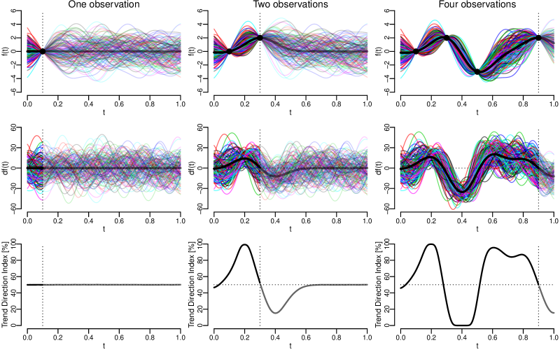
Figure 2: 150 realizations from the posterior distribution of $f$ (top row), $df$ (middle row) with expected values in bold and the Trend Direction Index (bottom row) conditional on one, two and four noise free observations. Dotted vertical lines show the points in time after which forecasting takes place.

The Trend Direction Index is illustrated in Figure 2 in the noise free case, $\sigma=0$, with known values of $\bm{\beta}$ and $\bm{\theta}$, and where the prior expected value of $f$ is set equal to $\mu_{\bm{\beta}}(t)=0$. The first and second rows of the plot show 150 random sample paths from the posterior distribution of $(f,df)$ with the posterior expectations in bold lines, and the third row shows the Trend Direction Index. Since the hyper-parameters, $\bm{\Theta}$, are known in this example, the Trend Direction Index is a deterministic function of time. The three columns in the plot show how the posteriors of $f$, $df$, and $\mathrm{TDI}$ are updated after one, two and four observations both forwards and backwards in time. The figure shows how the inclusion of additional observations results in changes of the posterior distribution of the trend and the Trend Direction Index. The uncertainty of the forecasts remains unchanged, whereas the posterior distributions back in time restricts the uncertainty of the curves to accommodate the observations. The vertical dotted lines denote the point in time after which forecasting occurs. When forecasting beyond the last observation, the posterior of $f$ becomes more and more dominated by its prior implying that $df$ becomes symmetric around zero so that the Trend Direction Index stabilizes around $50\%$.

2.3 The Expected Trend Instability

The Expected Trend Instability was defined in Equation (2) as the expected number of roots of the trend on an interval conditional on observed data. Now we make this concept more precise and frame it in the context of the latent Gaussian Process model. Let $\mathcal{I}$ be a compact subset of the real line and consider the random càdlàg function

$$N_{\mathcal{I}}(t)=\#\left\{s\leq t:df(s)=0,s\in\mathcal{I}\right\}$$

counting the cumulative number of points in $\mathcal{I}$ up to time $t$ where the trend is equal to zero. The Expected Trend Instability on $\mathcal{I}$ is equal to

$$\mathrm{ETI}(\mathcal{I}\mid\bm{\Theta})=\mathop{\mathrm{E}}\left[N_{\mathcal{I}}\left(\max\mathcal{I}\right)\mid\bm{\Theta},\mathcal{F}\right]$$

giving the expected number of zero-crossings by $df$ on $\mathcal{I}$. The following proposition gives the expression for the Expected Trend Instability under the data generating model in Equation (3).

Proposition 3.

Let $\mathcal{F}$ be the $\sigma$-algebra generated by the observed data $(\mathbf{Y},\mathbf{t})$ and $\mu_{df}$, $\mu_{d^{2}\!f}$, $\Sigma_{df}$, $\Sigma_{d^{2}\!f}$ and $\Sigma_{df,d^{2}\!f}$ the moments of the joint posterior distribution of $(df,d^{2}\!f)$ as stated in Proposition 1, and assume that all assumptions A1-A4 are fulfilled. The Expected Trend Instability is then

$$\mathrm{ETI}(\mathcal{I}\mid\bm{\Theta})=\int_{\mathcal{I}}d\mathrm{ETI}(t\mid\Theta)\mathrm{d}t$$

where $d\mathrm{ETI}$ is the local Expected Trend Instability given by

$$d\mathrm{ETI}(t,\mathcal{T}\mid\bm{\Theta})=\lambda(t\mid\Theta)\phi\left(\frac{\mu_{df}(t\mid\bm{\Theta})}{\Sigma_{df}(t,t\mid\bm{\Theta})^{1/2}}\right)\left(2\phi(\zeta(t\mid\bm{\Theta}))+\zeta(t\mid\bm{\Theta})\mathop{\mathrm{Erf}}\left(\frac{\zeta(t\mid\bm{\Theta})}{2^{1/2}}\right)\right)$$

and $\phi\colon\,x\mapsto 2^{-1/2}\pi^{-1/2}\exp(-\frac{1}{2}x^{2})$ is the standard normal density function, $\mathop{\mathrm{Erf}}\colon\,x\mapsto 2\pi^{-1/2}\int_{0}^{x}\exp(-u^{2})\mathrm{d}u$ is the error function, and $\lambda$, $\omega$ and $\zeta$ are functions defined as

$$\lambda(t\mid\Theta) =\frac{\Sigma_{d^{2}\!f}(t,t\mid\bm{\Theta})^{1/2}}{\Sigma_{df}(t,t\mid\bm{\Theta})^{1/2}}\left(1-\omega(t\mid\bm{\Theta})^{2}\right)^{1/2}$$

$$\omega(t\mid\bm{\Theta}) =\frac{\Sigma_{df,d^{2}\!f}(t,t\mid\bm{\Theta})}{\Sigma_{df}(t,t\mid\bm{\Theta})^{1/2}\Sigma_{d^{2}\!f}(t,t\mid\bm{\Theta})^{1/2}}$$

$$\zeta(t\mid\bm{\Theta}) =\frac{\mu_{df}(t\mid\bm{\Theta})\Sigma_{d^{2}\!f}(t,t\mid\bm{\Theta})^{1/2}\omega(t)\Sigma_{df}(t,t\mid\bm{\Theta})^{-1/2}-\mu_{d^{2}\!f}(t\mid\bm{\Theta})}{\Sigma_{d^{2}\!f}(t,t\mid\bm{\Theta})^{1/2}\left(1-\omega(t\mid\bm{\Theta})^{2}\right)^{1/2}}$$

To illustrate the Expected Trend Instability, Figure 3 shows $25$ random Gaussian Processes on the unit interval simulated under three different values of $\mathrm{ETI}$. The sample paths are paired so that each function in the first row has an associated trend in the second row. The different values of $\mathrm{ETI}$ are set to $0.25$, $0.5$ and $1$ corresponding to the expected number of times that the functions change monotonicity or equivalently that the trend crosses zero on that interval. Sample paths that are trend stable, i.e., always increasing/decreasing, are shown by solid blue lines, and sample paths that are trend unstable, i.e., the derivatives crosses zero, are shown by dashed gold colored lines. It is seen that for low values of $\mathrm{ETI}$ most of the sample paths preserve their monotonicity on the interval and their associated derivatives are correspondingly either always positive or negative. For larger values of $\mathrm{ETI}$, more of the trends start crossing zero implying less stability in the monotonicity of $f$. We note that even though we are only modeling a single curve, the Expected Trend Instability is defined in terms of a posterior distribution of random curves which is what the figure illustrates.

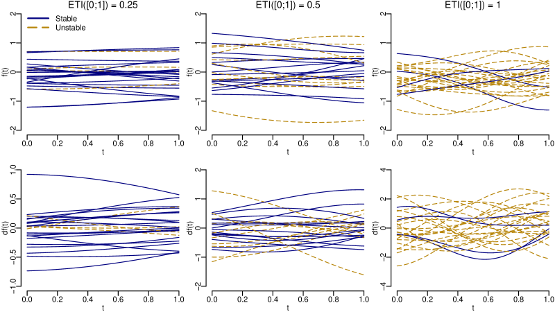
Figure 3: $25$ random pairs sampled from the joint distribution of a Gaussian Process ($f$) and its derivative ($df$) with different values of Expected Trend Instability (ETI). The first row shows samples from $f$, and the second row shows samples from $df$. The columns define different values of ETI. Sample paths that are trend stable are shown by solid blue lines, and unstable sample paths are shown by dashed gold colored lines.

2.4 Modeling the prior

To complete the model specification in Equation (3) we must decide on the functional forms of the mean and covariance functions of the Gaussian Process prior, but there is an inherent ambiguity in how to choose these. To explain this issue we note that a square-integrable Gaussian Process on a compact domain can by written as $f(t)=\mu_{\beta}(t)+\sum_{p=1}^{\infty}Z_{p}\phi_{p}(t)$ where $Z_{p}$ are independent, zero mean and unit variance normally distributed random variables, and $\phi_{p}$ are pair-wise orthonormal functions. This is known as the Karhunen–Loève representation. Furthermore, Mercer’s theorem states that any continuous covariance function admits the representation $C(s,t)=\sum_{p=1}^{\infty}\lambda_{p}\phi_{p}(s)\phi_{p}(t)$ uniformly on $\mathcal{T}\times\mathcal{T}$ where $\phi_{p}$ are the eigen-functions of $C$ and form an orthonormal basis of $L^{2}$. This shows that $f$ can be written as a sum of its mean and a possibly infinite weighted sum of functions defined implicitly through the spectral decomposition of the covariance function. So if e.g., the linear function is an eigen-function of the covariance function it will be superfluous in the mean. This results in a trade-off situation where a rich specification of the mean, $\mu_{\beta}$, gives little space for flexibility added by the covariance function, $C$. On the other hand, a spartan mean structure requires a flexible covariance structure. The latter approach is prevalent in applied Gaussian Process regression modeling where a very simple mean structure (often just a constant or linear term) is used in the prior but in combination with a flexible covariance function. We refer to Kaufman et al. (2011) for further discussions of these issues. We note that this issue arises because our approach focuses on a single realization of a random function. In the case of multiple observations of $f$ the issue would be different.

Regarding the choice of covariance function, the Squared Exponential (SE), the Rational Quadratic (RQ), the Matern 3/2 (M3/2), and the Matern 5/2 (M5/2) are commonly used covariance functions for Gaussian Process regression (Rasmussen and Williams 2006). These covariance functions are given by

$$\begin{split}C_{\bm{\theta}}^{\text{SE}}(s,t)&=\alpha^{2}\exp\left(-\frac{(s-t)^{2}}{2\rho^{2}}\right),\quad\bm{\theta}=(\alpha,\rho)>0\\ C_{\bm{\theta}}^{\text{RQ}}(s,t)&=\alpha^{2}\left(1+\frac{(s-t)^{2}}{2\rho^{2}\nu}\right)^{-\nu},\quad\bm{\theta}=(\alpha,\rho,\nu)>0\\ C_{\bm{\theta}}^{\text{M3/2}}(s,t)&=\alpha^{2}\left(1+\frac{\sqrt{3}\sqrt{(s-t)^{2}}}{\rho}\right)\exp\left(-\frac{\sqrt{3}\sqrt{(s-t)^{2}}}{\rho}\right),\quad\bm{\theta}=(\alpha,\rho)>0\\ C_{\bm{\theta}}^{\text{M5/2}}(s,t)&=\alpha^{2}\left(1+\frac{\sqrt{5}\sqrt{(s-t)^{2}}}{\rho}+\frac{5(s-t)^{2}}{3\rho^{2}}\right)\exp\left(-\frac{\sqrt{5}\sqrt{(s-t)^{2}}}{\rho}\right),\quad\bm{\theta}=(\alpha,\rho)>0\end{split}$$ (6)

The SE covariance function gives rise to very smooth functions due to it being infinitely differentiable. This can be disadvantageous in some applications as that will make it difficult for the posterior to adapt to localized changes in smoothness. The other listed covariance functions try to remedy this issue. Specifically, the RQ covariance function can be derived as an infinite scale mixture of SE covariance functions in terms of $\rho^{-2}$. This enables the resulting estimates to operate on different time scales simultaneously. Smaller values of $\nu$ will give rise to more wiggly posteriors, and as it is one of the model’s hyper-parameters its value and the implied adaptivity will be data-driven. For $\nu\rightarrow\infty$ the RQ covariance function converges on $\mathcal{T}\times\mathcal{T}$ to the SE covariance function. The Matern covariance functions shown here explicitly for a generally continuous parameter $\nu=3/2$ and $\nu=5/2$ belong to a larger class of covariance functions. The general expression is involved and includes a modified Bessel function for which derivatives are difficult to calculate. In this class of covariance functions $\nu$ directly controls the differentiability which again can be chosen in a data-driven manner.

If non-stationary components are suspected to be presented in the data generating process, these can be included in the covariance structure as part of defining the prior. One example is the non-stationary covariance function for periodic components discussed by MacKay (1998). Another noteworthy example is the neural network covariance structure of Williams (1998). In fact, Neal (2012) showed that a Bayesian neural network with one hidden layer converges to a Gaussian Process when the number of hidden neurons goes to infinity. The actual form of covariance function implied by the neural network depends on the prior for the network weights and the activation functions.

It should be noted that sums and products of covariance functions produce valid covariance functions. Thus, a very wide range of flexible covariance structures can be constructed from simpler building blocks.

We conclude this section by noting two covariance functions that cannot be used in our model. This is because they are both in violation with Assumption A3 which can be verified by a straight-forward calculation. The first case is the M3/2 covariance function in Equation (6). While it can be used to estimate the Trend Direction Index, it cannot be used if an estimate of the Expected Trend Instability is also required. Another example is $C_{\bm{\theta}}^{\text{OU}}(s,t)=\alpha^{2}\exp\left(-|s-t|/\rho\right)$. This is the covariance function of the Ornstein-Uhlenbeck process which is mean-squared continuous but not mean-squared differentiable. This also fails to satisfy the required assumption.

2.5 The Gaussian assumptions and non-normal outcomes

The closed-form expressions derived above depend on the assumptions of normality on the latent scale and for the conditional distribution of the observed data. For outcomes that are conditionally non-normal the posterior distributions are in general analytically intractable. In some cases one can see our assumptions as an approximation facilitated by the central limit theorem e.g., in the case where the outcome is a proportion and the number of experiments is large, or if the outcome is count data and the rate is not too low. The conditional variance, $\sigma^{2}$ in Equation (3), can therefore be changed to reflect the structure of the variance of such limiting distribution.

One possibility for altering the model is to retain the structure but apply a transformation of the observed data. This amounts to altering the second part of Equation (3) to

$$g(Y_{i})\mid t_{i},f(t_{i}),\bm{\Theta} \overset{iid}{\sim}N(f(t_{i}),\sigma^{2})$$

where $g$ is a known, monotone function. Our model could directly be fitted to the transformed outcomes, but the posterior estimates will also be on the transformed scale and may therefore be difficult to interpret.

Another possibility is to consider both the outcome and the latent function on the same transformed scale. This alters Equation (3) to

$$\begin{split}g(f)\mid\bm{\beta},\bm{\theta}&\sim\mathcal{GP}(\mu_{\bm{\beta}}(\cdot),C_{\bm{\theta}}(\cdot,\cdot))\\ g(Y_{i})\mid t_{i},g(f(t_{i})),\bm{\Theta}&\overset{iid}{\sim}N(g(f(t_{i})),\sigma^{2})\end{split}$$

Our model is again directly applicable under this alternative data generating model. It follows that the trend on this scale is $g(f(t))^{\prime}=f^{\prime}(t)g^{\prime}(f(t))$, and the Trend Direction Index will therefore be equal to $\mathrm{TDI}(t,\delta\mid\bm{\Theta})=P(f^{\prime}(t+\delta)g^{\prime}(f(t+\delta))>0\mid g(\mathbf{Y}),\mathbf{t},\bm{\Theta})$. This can, however, be transformed back to the original scale of $df$ by normalization since we can sample from the posterior distribution of $g(f(t))$ by the Gaussian assumptions on the transformed scale. Therefore, it is also possible to obtain samples from $g^{\prime}(f(t))$ as $g^{-1}$ and $g^{\prime}$ are known. The Trend Direction Index on the original scale can in this way be obtained by a Monte Carlo approximation using the transformed samples.

3 Estimation

The trend indices depend on the hyper-parameters, $\bm{\Theta}$, of the latent Gaussian Process. These must be estimated from the observed data, and we consider two different estimation procedures: maximum likelihood estimation and a fully Bayesian estimator.

The difference between the maximum likelihood and the Bayesian method is that they give rise to two different interpretations of the Trend Direction Index. In the former, the index is a deterministic function, while in the latter it is a random function governed by the posterior distribution of $\bm{\Theta}$. The maximum likelihood estimator is also known as the empirical Bayes approach since the hyper-parameters are estimated from data using the marginal likelihood of the model. This can be seen as an approximation to the Bayesian model where the hyper-parameters are fixed at their most likely values instead of being integrated out.

The maximum likelihood estimator consists of finding the values of the hyper-parameters that maximize the marginal likelihood of the observed data and plugging these into the expressions of the posterior distributions and the trend indices. The marginal distribution of $\mathbf{Y}$ can be found by integrating out the distribution of the latent Gaussian Process in the conditional specification $\mathbf{Y}\mid f(\mathbf{t}),\mathbf{t},\bm{\Theta}$ in Equation (3). Since the observation model consists of normal distributed random variables conditional on the latent Gaussian Process, the marginal distribution is multivariate normal with expectation $\mu_{\bm{\beta}}(\mathbf{t})$ and $n\times n$ covariance matrix $C_{\bm{\theta}}(\mathbf{t},\mathbf{t})+\sigma^{2}I$. The marginal log-likelihood function is therefore

$$\log L(\bm{\Theta}\mid\mathbf{Y},\mathbf{t}) \propto-\frac{1}{2}\log|C_{\bm{\theta}}(\mathbf{t},\mathbf{t})+\sigma^{2}I|-\frac{1}{2}(\mathbf{Y}-\mu_{\bm{\beta}}(\mathbf{t}))^{T}\left[C_{\bm{\theta}}(\mathbf{t},\mathbf{t})+\sigma^{2}I\right]^{-1}(\mathbf{Y}-\mu_{\bm{\beta}}(\mathbf{t}))$$ (7)

and the maximum likelihood estimate $\widehat{\bm{\Theta}^{\text{ML}}}=\mathop{\mathrm{arg\,sup}}_{\bm{\Theta}=(\bm{\beta},\bm{\theta},\sigma)}\log L(\bm{\Theta}\mid\mathbf{Y},\mathbf{t})$ can be obtained by numerical optimization or found as the roots to the score equations $\nabla_{\bm{\Theta}}\log L(\bm{\Theta}\mid\mathbf{Y},\mathbf{t})=0$. This estimate can be plugged in to the expressions for the posterior distributions of $(f,df,d^{2}\!f)$ in Proposition 1 enabling simulation of the posterior distributions at any vector of time points. Estimates of the Trend Direction Index and the Expected Trend Instability are similarly $\mathrm{TDI}(t,\delta\mid\widehat{\bm{\Theta}^{\text{ML}}})$ and $\mathrm{ETI}(\mathcal{I}\mid\widehat{\bm{\Theta}^{\text{ML}}})$ according to Propositions 2 and 3 respectively, and the predictive distribution of a new observation is equal to Equation (5) with the plug-in estimate $\bm{\Theta}=\widehat{\bm{\Theta}^{\text{ML}}}$.

The maximum likelihood estimator is easy to implement and fast to compute, but it is difficult to propagate the uncertainties of the parameter estimates through to the posterior distributions and the trend indices. This is disadvantageous since in order to conduct a qualified assessment of trendiness we are not only interested in point estimates but also the associated uncertainties. A Bayesian estimator, while slower to compute, facilitates a straightforward way to encompass all uncertainties in the final estimates. To specify a Bayesian estimator we must augment the data generating model in Equation (3) with another hierarchical level specifying the prior distribution of the hyper-parameters. We therefore add the following level

$$(\bm{\beta},\bm{\theta},\sigma)\sim G(\bm{\Theta}\mid\bm{\Psi},\mathbf{t})$$

to the specification where $G$ is some family of distribution indexed by a vector $\bm{\Psi}$. The joint distribution of the model can be factorized as

$$P(\mathbf{Y},f(\mathbf{t}),\bm{\Theta}\mid\bm{\Psi},\mathbf{t})=P(\mathbf{Y}\mid f(\mathbf{t}),\bm{\Theta},\bm{\Psi},\mathbf{t})P(f(\mathbf{t})\mid\bm{\Theta},\bm{\Psi},\mathbf{t})G(\bm{\Theta}\mid\bm{\Psi},\mathbf{t})$$

and each conditional probability is specified by a sub-model in the augmented hierarchy. We always condition on $\bm{\Psi}$ and $\mathbf{t}$ as they are considered fixed. The posterior distribution of the hyper-parameters given the observed data is then

$$\begin{split}P(\bm{\Theta}\mid\mathbf{Y},\bm{\Psi},\mathbf{t})&=\frac{G(\bm{\Theta}\mid\bm{\Psi},\mathbf{t})P(\mathbf{Y}\mid\bm{\Theta},\bm{\Psi},\mathbf{t})}{P(\mathbf{Y}\mid\bm{\Psi},\mathbf{t})}\\ &=\frac{G(\bm{\Theta}\mid\bm{\Psi},\mathbf{t})\int P(\mathbf{Y}\mid f(\mathbf{t}),\bm{\Theta},\bm{\Psi},\mathbf{t})dP(f(\mathbf{t})\mid\bm{\Theta},\bm{\Psi},\mathbf{t})}{\iint P(\mathbf{Y}\mid f(\mathbf{t}),\bm{\Theta},\bm{\Psi},\mathbf{t})dP(f(\mathbf{t})\mid\bm{\Theta},\bm{\Psi},\mathbf{t})dG(\bm{\Theta}\mid\bm{\Psi},\mathbf{t})}\end{split}$$ (8)

and we let $\widetilde{\bm{\Theta}}\sim P(\bm{\Theta}\mid\mathbf{Y},\bm{\Psi},\mathbf{t})$. The posterior distribution of $\bm{\Theta}$ induces corresponding distributions over the trend indices according to $\mathrm{TDI}(t,\delta\mid\widetilde{\bm{\Theta}})$, $d\mathrm{EDI}(t,\mathcal{T},\mid\widetilde{\bm{\Theta}})$ and $\mathrm{EDI}(\mathcal{I}\mid\widetilde{\bm{\Theta}})$. For example, the Trend Direction Index in the Bayesian formulation is a surface in $(t,\delta)$ where each value is a distribution over probabilities. We suggest to summarize the trend indices by their posterior quantiles. For the Trend Direction Index we summarize its posterior distribution by functions $Q_{\tau}$ such that

$$P\left(\mathrm{TDI}\left(t,\delta\mid\widetilde{\bm{\Theta}}\right)\leq\tau\right)=Q_{\tau}(t,\delta)$$

with for example $\tau\in\left\{0.025,0.5,0.975\right\}$ to obtain 95% credible intervals. In the Bayesian model the predictive distribution in Equation (5) should be averaged across the posterior distribution of the hyper-parameters. This leads to the posterior predictive distribution

$$Y^{\ast}(t^{\ast})\mid t^{\ast},\mathbf{Y},\mathbf{t},\bm{\Psi}=\int_{\bm{\Theta}}P(Y^{\ast}(t^{\ast})\mid t^{\ast},\mathbf{Y},\mathbf{t},\bm{\Theta},\bm{\Psi})dP(\bm{\Theta}\mid\mathbf{Y},\bm{\Psi},\mathbf{t})$$

where the integral is in practice approximated through the MCMC samples.

We have implemented both the maximum likelihood and the Bayesian estimator in Stan (Carpenter et al. 2017) and R (R Core Team 2018) in combination with the rstan package (Stan Development Team 2018). Stan is a probabilistic programming language enabling fully Bayesian inference using Markov chain Monte Carlo sampling. The Stan implementation of the maximum likelihood estimator requires the marginal maximum likelihood estimates of the parameters supplied as data, and from these it will simulate random realizations of the posterior distribution of $(f,df,d^{2}\!f)$ on a user-supplied grid of time points and return point estimates of $\mathrm{TDI}$ and $d\mathrm{ETI}$. The latter can then be integrated numerically to obtain the Expected Trend Instability on an interval. The Bayesian estimator requires a specification of $\bm{\Psi}$ supplied as data and from that it will generate realizations of $(\widetilde{\bm{\Theta}}_{1},\ldots,\widetilde{\bm{\Theta}}_{K})$ from Equation (8). These samples are then used to obtain the posterior distribution of the Trend Direction Index by $(\mathrm{TDI}(t,\delta\mid\widetilde{\bm{\Theta}}_{1}),\ldots,\mathrm{TDI}(t,\delta\mid\widetilde{\bm{\Theta}}_{K}))$ and similarly for $d\mathrm{ETI}$ according to Propositions 2 and 3.

3.1 Model selection

In connection with Section 2.4 on choosing the mean and covariance structure for the Gaussian Process prior we propose a practical approach based on specifying a set of candidate models and choosing the best fitting model among these according to a cross-validation procedure. Different types of cross-validation can be performed depending on the purpose of the analysis. In some cases one stands at the end of the data collection and wants to look at what has been observed. In this cases it would be natural to condition on all the observed data and perform leave-one-out cross-validation. In other cases one is interested in forecasting the trend and the associated indices, and here it would be natural to take the direction of time into account. This could be done by e.g., performing one-step-ahead cross-validation in which the observed data are compared to a sequence of models forecasting one step ahead in time based on successive partitioning of the time series. For more information on such procedures see e.g., Bergmeir and Benítez (2012).

To perform the leave-one-out cross-validation we consider a set of candidate models indexed by $\mathcal{M}$. This set would typically include different parameterizations of the mean and covariance function of $f$. Turn by turn, a single data pair $(Y_{i},t_{i})$ is excluded, and we let the corresponding leave-one-out data be denoted $(\mathbf{Y}_{-i},\mathbf{t}_{-i})$. Based on the leave-one-out data the hyper-parameters are estimated for each model by maximizing the marginal log-likelihood in Equation (7) and given by

$$\widehat{\bm{\Theta}}_{-i}^{\mathcal{M}}=\mathop{\mathrm{arg\,sup}}_{\bm{\Theta}}\log L(\bm{\Theta}\mid\mathbf{Y}_{-i},\mathbf{t}_{-i})$$

Plugging these estimates into the expression for the posterior expectation of $f$ in Proposition 1 we obtain the leave-one-out predictions, and the mean squared error of prediction (or another loss function) can be calculated by comparing the predictions and the observed values averaged across all data points as

$$\text{MSPE}_{\text{LOO}}^{\mathcal{M}}=\frac{1}{n}\sum_{i=1}^{n}\left(Y_{i}-\mathop{\mathrm{E}}[f(t_{i})\mid\mathbf{Y}_{-i},\mathbf{t}_{-i},\widehat{\bm{\Theta}}_{-i}^{\mathcal{M}}]\right)^{2}$$

The selected model among the candidate set is $\mathcal{M}_{\text{opt}}=\mathop{\mathrm{arg\,min}}_{\mathcal{M}}\text{MSPE}_{\text{LOO}}^{\mathcal{M}}$. Different cross-validation schemes can be performed in a similar manner by modifying how the leave-one-out data sets are constructed.

We note that with our model being implemented in Stan, efficient approximate leave-one-out cross-validation and model comparison using the LOOIC criterion can be directly performed with the loo package (Vehtari et al. 2019).

4 Simulation study

To assess the performance of our method we performed a simulation study. We generated $r=1,\ldots,10,000$ random Gaussian Processes on the unit interval with zero mean and the Squared Exponential (SE) covariance function (see Equation (6)) with parameters $\alpha=1$ and $\rho=\frac{\sqrt{3}}{{2\pi}}$ in 15 different scenarios in which we varied the number of observation points ($n=25,50,100$) and the measurement noise ($\sigma=0.025,0.05,0.1,0.15,0.2$). The Supplementary Material shows 50 random sample paths for each scenario.

In each of the $r$ simulations we know the true latent functions $(f_{r},df_{r})$, and by fitting our model we obtain estimates $\widehat{f_{r}^{\text{GP}}}$ and $\widehat{df_{r}^{\text{GP}}}$ corresponding to the posterior expectations in Proposition 1, and $\mathrm{TDI}_{r}$ and $d\mathrm{ETI}_{r}$ from Propositions 2 and 3. We compare these estimates to the truths using two different measures: an integrated residual and the squared $L^{2}$ norm. The integrated residuals are defined as $\int_{0}^{1}(f_{r}(t)-\widehat{f_{r}^{\text{GP}}}(t))\mathrm{d}t$ and similarly for $\widehat{df_{r}^{\text{GP}}}$. For the Trend Direction Index the cumulative residual is defined as $\int_{0}^{1}(1(df_{r}(t)>0)-\mathrm{TDI}_{r}(t))\mathrm{d}t$ where $1$ denotes the indicator function. For the Expected Trend Instability the cumulative residual is defined as $\int_{0}^{1}(N_{r}(t)-d\mathrm{ETI}_{r}(t))\mathrm{d}t$ where $N_{r}(t)$ is the càdlàg counting process that jumps with a value of 1 every time $df_{r}$ has a root on the interval. If our estimates are unbiased we expect these integrated residuals to have zero mean across the simulations. The squared $L^{2}$ norms are defined in a similar manner for all the quantities as e.g., $\int_{0}^{1}(f_{r}(t)-\widehat{f_{r}^{\text{GP}}}(t))^{2}\mathrm{d}t$ and reflect the variability of the estimates.

For comparison we employed the Trend Filtering method implemented in the R package genlasso (Arnold and Tibshirani 2019) on the same simulated data and reported similar measures for its estimated mean, $\widehat{f^{\text{TF}}}$, and derivative, $\widehat{df^{\text{TF}}}$, using 10-fold cross-validation of the penalty parameter. We only compare the estimates of the latent mean and its derivative between the two approaches as Trend Filtering does not provide a probability distribution for the derivative.

Summary statistics from the simulation study are shown in Table 1. It is seen that both our model and Trend Filtering provide unbiased estimates in all scenarios. Looking at the squared $L^{2}$ norm our estimates of $f$ and $df$ show very small variability across all scenarios, while the estimates from Trend Filtering showed an increase in variability for increasing measurement noise and a decrease for increasing number of observations. This is expected as we simulate random functions with continuous sample paths, and Trend Filtering estimates piece-wise linear approximations. While this leads to unbiased estimates, the variability of these estimates are larger, and this is more pronounced for smaller number of observations.

The variability of the Trend Direction Index and the Expected Trend Instability as measured by the squared $L^{2}$ norm were low in all scenarios but increased with the magnitude of the measurement noise as expected. In a few cases the estimated Expected Trend Instability was far away from its true value. This was especially pronounced in scenarios with a small number of observations and a high measurement noise. The reason was that $\widehat{f^{\text{GP}}}$ degenerated to either a constant function or to a perfect interpolation of the observed data. This is a consequence of the hyper-parameters being weakly identified under such circumstances. These cases are still part of the reported summary statistics in Table 1. For such cases, the model fit can be regularized through the priors of the hyper-parameters, but this must be determined on a case-by-case basis.

Table 1: Summary statistics from the simulation study. Each value is the mean across 10,000 simulations except for ETI where the median is reported. Superscript GP denotes our proposed method and TF denotes Trend Filtering. Numbers have been rounded to three decimal places.

		Integrated residual						Squared L2 norm
n	$\sigma$	$\widehat{f^{\text{GP}}}$	$\widehat{df^{\text{GP}}}$	$\widehat{f^{\text{TF}}}$	$\widehat{df^{\text{TF}}}$	TDI	ETI	$\widehat{f^{\text{GP}}}$	$\widehat{df^{\text{GP}}}$	$\widehat{f^{\text{TF}}}$	$\widehat{df^{\text{TF}}}$	TDI	ETI
25	0.025	0	0	0.000	0.000	0.000	0.000	0.000	0.000	0.041	0.504	0.011	0.008
25	0.050	0	0	0.000	0.000	0.000	-0.002	0.001	0.001	0.130	1.188	0.021	0.018
25	0.100	0	0	0.002	0.003	0.001	-0.008	0.003	0.004	0.408	2.988	0.037	0.040
25	0.150	0	0	-0.001	-0.002	-0.001	-0.020	0.005	0.008	0.818	5.248	0.051	0.064
25	0.200	0	0	-0.003	-0.003	-0.001	-0.034	0.009	0.014	1.343	8.248	0.063	0.094
50	0.025	0	0	0.000	0.000	0.000	0.000	0.000	0.000	0.026	0.535	0.009	0.006
50	0.050	0	0	0.000	0.000	0.000	-0.002	0.000	0.001	0.081	1.287	0.016	0.012
50	0.100	0	0	0.000	0.000	0.000	-0.006	0.001	0.002	0.244	3.348	0.028	0.028
50	0.150	0	0	0.000	0.001	0.000	-0.012	0.003	0.005	0.469	6.353	0.038	0.045
50	0.200	0	0	0.000	0.003	0.001	-0.020	0.005	0.008	0.759	9.832	0.050	0.068
100	0.025	0	0	0.000	0.000	0.000	0.000	0.000	0.000	0.016	0.399	0.007	0.004
100	0.050	0	0	0.000	0.001	0.000	-0.001	0.000	0.000	0.050	1.020	0.012	0.009
100	0.100	0	0	0.000	0.000	0.000	-0.003	0.001	0.001	0.150	2.187	0.022	0.019
100	0.150	0	0	0.000	-0.003	0.000	-0.007	0.002	0.002	0.283	4.454	0.030	0.031
100	0.200	0	0	0.002	0.002	0.001	-0.012	0.003	0.004	0.450	6.140	0.038	0.045

5 Applications

Trend of proportion of Danish smokers

A report published by The Danish Health Authority in January 2019 updated the estimated proportion of daily or occasional smokers in Denmark with new data from 2018 (The Danish Health Authority 2019). The data was based on an online survey including 5017 participants. The report also included data on the proportion of smokers in Denmark during the last 20 years which was shown in Figure 1. The report was picked up by several news papers under headlines stating that the proportion of smokers in Denmark had significantly increased for the first time in two decades (Navne, Schmidt, and Rasmussen 2019). The report published no statistical analyses for this statement but wrote, that because the study population is so large, then more or less all differences become statistically significant at the $5\%$ level (this was written as a $95\%$ significance level in the report).

This data set provides an instrumental way of exemplifying our two proposed measures of trendiness. In this application we wish to assess the statistical properties of the following questions:

• Is the proportion of smokers increasing in the year 2018 conditional on data from the last 20 years?

• If the proportion of smokers is currently increasing, when did this increase probably start?

• Is it the first time during the last 20 years that the trend in the proportion of smokers has changed?

A naive approach for trying to answer questions Q1 and Q2 is to apply sequential $\chi^{2}$-tests in a $2\times 2$ table. Table 2 shows the p-values for the $\chi^{2}$-test of independence between the proportion of smokers in 2018 and each of the five previous years. Using a significance level of $5\%$ the conclusion is ambiguous. Compared to the previous year, there was no significant change in the proportion in 2018. Three out of these five comparisons fail to show a significant change in proportions. It is therefore evident that such point-wise testing is not sufficiently perceptive to catch the underlying continuous development.

	2017	2016	2015	2014	2013
p-value	0.074	0.020	0.495	0.012	0.576

Table 2: p-values obtained from $\chi^{2}$-tests of independence between the proportion of smokers in 2018 and the five previous years. Numbers in bold are statistically significant differences at the $5\%$ level.

Similarly, a simple approach for trying to answer question Q3 would be to look at the cumulative number of times that the difference in proportion between consecutive years changes sign. In the data set there were nine changes in the sign of the difference between the proportion in each year and the proportion in the previous year giving this very crude estimate of the number of times that the trend has changed. This approach suffers from the facts that it is based on a finite difference approximation at the sampling points to the continuous derivative, and that it uses the noisy measurements instead the latent function. Consequently, the changes in trend are quite unstable.

We now present an analysis of the data set using our method. As a specification of the latent function we considered three different mean functions, a constant mean $\mu_{\bm{\beta}}(t)=\beta_{0}$, a linear mean $\mu_{\bm{\beta}}(t)=\beta_{0}+\beta_{1}t$, and a quadratic mean $\mu_{\bm{\beta}}(t)=\beta_{0}+\beta_{1}t+\beta_{2}t^{2}$ and the four different covariance functions given in Equation (6). This gives a total of 12 different candidate models to compare. Since we condition on all the observed data and are not interested in forecasting in this application we performed the model comparison by leave-one-out cross-validation as discussed in Section 3.1.

Table 3 shows the mean squared error of prediction for each candidate model. For the models with a Rational Quadratic covariance function and a linear and a quadratic mean function the parameter $\nu$ diverged numerically implying convergence to the Squared Exponential covariance function. Comparing the leave-one-out mean squared error of prediction, the prior distribution of $f$ in the optimal model has a constant mean function and a Rational Quadratic covariance function. The marginal maximum likelihood estimates of the parameters in the optimal model were

$$\widehat{\beta_{0}^{\text{ML}}}=28.001,\quad\widehat{\alpha^{\text{ML}}}=4.543,\quad\widehat{\rho^{\text{ML}}}=4.438,\quad\widehat{\nu^{\text{ML}}}=1.020,\quad\widehat{\sigma^{\text{ML}}}=0.622$$ (9)

	SE	RQ	Matern 3/2	Matern 5/2
Constant	0.682	0.651	0.687	0.660
Linear	0.806	$\Leftarrow$	0.896	0.865
Quadratic	0.736	$\Leftarrow$	0.800	0.785

Table 3: Leave-one-out cross-validated mean squared error of prediction for each of the 12 candidate models. $\Leftarrow$ indicates numerical convergence to the SE covariance function.

Figure 4 shows the fit of the model by the maximum likelihood method. The plots were obtained by plugging the maximum likelihood estimates into the expressions for the posterior distributions of $f$ and $df$ defined in Proposition 1, the Trend Direction Index in Proposition 2, and the Expected Trend Instability in Proposition 3. The predictions were performed on an equidistant grid of $500$ time points spanning the 20 years. The plot of the posterior trend (top right) shows two regions in time where the posterior mean of the derivative is positive, one around $[2004;2008]$ and one shortly after $2015$ and until the end of the observation period. The Trend Direction Index (bottom left) quantifies this positive trendiness as a probability standing in $2018$ and looking back in time while also taking the uncertainty into account. The bottom right panel shows the local Expected Trend Instability and its integral is to the expected number of times that the trend has changed sign. Table 4 summarizes the maximum likelihood estimates of the Trend Direction Index at the end of the observation period and the previous five years as well as the Expected Trend Instability during the full observation period and during only the last ten years. Crosspoint is the first point in time during the last ten years where the Trend Direction Index became greater than $50\%$ i.e.,

$$\text{Crosspoint}=\mathop{\mathrm{arg\,min}}_{t\in[-10;0]}\left\{2018+t:\text{TDI}(2018,2018-t)\geq 50\%\right\}$$

Based on the results from the maximum likelihood analysis we may answer the questions by stating that the expected proportion of smokers in Denmark is currently increasing with a probability of $95.24\%$. This is, however, not a recent development as the probability of an increasing proportion has been greater than $50\%$ since the middle of 2015. This can be compared to the sequential $\chi^{2}$-tests in Table 2, which gave a cruder and less consistent result. The estimated values of $\mathrm{ETI}$ in Table 4 show that there has been an average of $3.68$ changes in the monotonicity of the proportion during the last 20 years. This value does support the statement by the news outlets that it is the first time in 20 years that the trend has changed. The value, however, reduces to 1.39 when only looking 10 years back, which is slightly less than half the ETI for the longer period.

Figure 4: Results from fitting the latent Gaussian Process model by maximum likelihood. The first row shows the posterior distributions of $f$ (left) and $df$ (right) with the posterior means in bold and gray areas showing point-wise probability intervals for the posterior distribution. The second row shows the estimated Trend Direction Index (left) and the local Expected Trend Instability (right).

We also applied the Bayesian estimator to the data using the same prior mean and covariance structure. The Bayesian estimator requires a prior distribution of the hyper-parameters. We used independent priors of the form

$$G(\bm{\Theta}\mid\bm{\Psi},\mathbf{t})=G(\beta_{0}\mid\Psi_{\beta_{0}},\mathbf{t})G(\alpha\mid\Psi_{\alpha},\mathbf{t})G(\rho\mid\Psi_{\rho},\mathbf{t})G(\nu\mid\Psi_{\nu},\mathbf{t})G(\sigma\mid\Psi_{\sigma},\mathbf{t})$$

where each prior was a heavy-tailed distribution with a moderate variance centered at the maximum likelihood estimates. We used the following distributions

$$\beta_{0} \sim T\left(\widehat{\beta_{0}^{\text{ML}}},3,3\right), \quad\alpha \sim\text{Half-}T\left(\widehat{\alpha^{\text{ML}}},3,3\right), \quad\rho \sim\text{Half-}N\left(\widehat{\rho^{\text{ML}}},1\right)$$

$$\nu \sim\text{Half-}T\left(\widehat{\nu^{\text{ML}}},3,3\right), \sigma \sim\text{Half-}T\left(\widehat{\sigma^{\text{ML}}},3,3\right)$$

where the maximum likelihood values are given in Equation (9) and $\text{Half-}T(\cdot,\cdot,\mathrm{df})$ and $\text{Half-}N(\cdot,\cdot)$ denotes the location-scale half T- and normal distribution functions with $\mathrm{df}$ degrees of freedom due to the requirement of positivity. We ran four independent Markov chains for 25,000 iterations each with half of the iterations used for warm-up and discarded. Convergence was assessed by trace plots of the MCMC draws and the potential scale reduction factor, $\widehat{R}$, of Gelman and Rubin (1992). The trace plots are included in the Supplementary Material.

Figure 5 shows the results from the Bayesian estimator. In this model both trend indices are time-varying posterior distributions and the top row of the shows the posterior distributions of the Trend Direction Index (left) and the Local Expected Trend Instability (right) summarized by time-dependent quantiles. The bottom row shows posterior density estimates of the Expected Trend Instability during the last twenty years (left) and during the last ten years (right). The same summary statistics as for the maximum likelihood analysis are given in Table 4 but here stated in terms of posterior medians and $2.5\%$ and $97.5\%$ posterior quantiles.

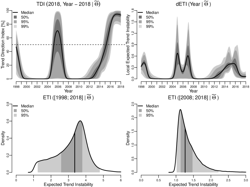
Figure 5: Results from fitting the latent Gaussian Process model by Bayesian analysis. The first row shows the posterior distributions of TDI (left) and local ETI (right) with the posterior means in bold and gray areas showing point-wise 95$\%$ and 99$\%$ probability intervals for the posterior distribution. The second row shows densities and probability intervals for the expected trend instability for the 20-year period back-in-time from 2018 (left) and 10 year back-in-time (right).

The results from the two analyses generally agree, but there are two differences that we wish to address. Both analyses showed a local peak in trendiness around 2006. In the maximum likelihood analysis this occurred at 2005.94 with a Trend Direction Index of $86.47\%$. In the Bayesian analysis the peak occurs at 2005.87 with a median Trend Direction Index of $79.43\%$ and a $95\%$ posterior probability interval of $[1.23\%;97.73\%]$. The added uncertainty estimates facilitated by the Bayesian estimator shows this trendiness is so variable that there is no reason to believe in a substantial increase in proportions at that point in time. This insight could not have been obtained from the maximum likelihood analysis.

The second difference is that the Bayesian model seems to generally induce more sluggish estimates due to mixing over the underlying parameters. This can be seen from the plot of the median local Expected Trend Instability in Figure 5 which is generally lower than its corresponding maximum likelihood point estimates in Figure 4. This is similarly reflected in the median ETI estimates in Table 4 which are lower than their values under maximum likelihood. Looking at the posterior distributions of the covariance parameters $\theta$ (not shown), we see that this is mainly a result of not restricting the parameter $\nu$ to its maximum likelihood value. The 95% probability interval of the posterior distribution of $\nu$ was $[0.328;10.743]$ which is highly right-skewed compared to the maximum likelihood estimate of $\widehat{\nu^{\text{ML}}}=1.020$.

To understand the effect of $\nu$ on the smoothness of the fitted models we can compare the local expected number of crossings by a Gaussian Process and its derivative at their mean values in the simple case of a zero-mean process with either the Rational Quadratic or the Squared Exponential covariance function. In this case the formula in Proposition 3 simplifies immensely, and as shown in the Supplementary Material the local expected number of mean-crossings by $f$ is equal to $\pi\rho^{-1}$ for both covariance functions. However, for $df$ the local expected number of mean-crossings is equal to $3^{1/2}\pi^{-1}\rho^{-1}$ for the Squared Exponential covariance function and $3^{1/2}\pi^{-1}\rho^{-1}(1+\nu^{-1})^{1/2}$ for the Rational Quadratic covariance function. We note that $1<(1+v^{-1})^{1/2}<\infty$ for $0<\nu<\infty$ and monotonically decreasing for $\nu\rightarrow\infty$ with a limit of one. Therefore, the value of $\nu$ has no effect on the crossing intensity of the process itself, but its derivative is always larger under a Rational Quadratic covariance function compared to the Squared Exponential covariance function with equality in the limit. A right-skewed posterior distribution of $\nu$ therefore favors fewer crossings of the trend leading to a more stable trend and a smaller value of the Expected Trend Instability.

	Maximum Likelihood	Bayesian Posterior
$\text{TDI}(2018,0)$	95.24%	93.32%	$[82.15\%;98.86\%]$
$\text{TDI}(2018,-1)$	95.92%	94.21%	$[84.28\%;99.11\%]$
$\text{TDI}(2018,-2)$	74.41%	77.87%	$[51.02\%;94.94\%]$
$\text{TDI}(2018,-3)$	33.36%	44.11%	$[18.23\%;69.19\%]$
$\text{TDI}(2018,-4)$	18.96%	20.60%	$[6.05\%;31.82\%]$
$\text{TDI}(2018,-5)$	9.50%	6.21%	$[0.03\%;22.21\%]$
Crosspoint	2015.48	2015.19	$[2014.62;2015.96]$
$\text{ETI}([1998,2018])$	3.68	3.36	$[1.24;4.79]$
$\text{ETI}([2008,2018])$	1.39	1.25	$[1.02;2.22]$

Table 4: Summary measures from the Maximum Likelihood and Bayesian analyses. The rows show the estimated Trend Direction Index for 2013 to 2018 and the Expected Trend Instability for the last 10 and 20 years all conditional on data from 1998 to 2018. For the Bayesian analysis posterior medians and 95$\%$ posterior probability intervals are given. Crosspoint is the time during the last $10$ years where $\mathrm{TDI}$ first exceeded $50\%$.

As a final remark to this application we note that the observed data are proportions and therefore by nature not normally distributed. Commonly used transformations for proportions towards normality are the isometric log ratio or the arcsine-square-root or logit functions. In accordance with Section 2.5 we also performed the trend analysis on the logit transformed outcomes. The results from this analysis are included in the Supplementary Material and did not give rise to different interpretations. This is perhaps not surprising as the observed proportions are far from the boundaries of the parameter space and consequently the normality approximation is more likely to hold.

Number of new COVID-19 positive cases in Italy

As a second application we look at the development of the number of new COVID-19 positives in Italy since February 24th 2020. Data was updated each day and made available at the GitHub repository of the Italian Civil Protection Department (Consiglio dei Ministri - Dipartimento della Protezione Civile 2020). 90 days had passed when this analysis was performed.

The data set provides a direct way to assess the COVID-19 disease progression and to monitor the impact of political initiatives to reduce disease spread. In this application we wish to assess the statistical properties of the following questions:

• Is the disease spread currently under control or does the number of new positive cases seems to be on the rise?

• How did the Italian government’s decision to lockdown most of Italy on March 9th 2020 reflect in the spread of the virus?

For this application we fitted the Gaussian Process model using the maximum likelihood method and as hyper-parameters we used a constant mean function and the Rational Quadratic covariance function.

Figure 6 shows the result of the analysis. Between day five and six the Trend Direction Index crossed 95% probability and continued to climb to 100%. After 29 days (March 24th, 2020) the index proceeded to sharply decrease where it remained for some time. The Italian government imposed a quarantine on most of Italy from March 9th, and the sharp drop coincides nicely with the (as of present) expected incubation period of 2–14 days which roughly reflects the incubation and testing period for the individuals who contracted the virus before the March 9th lockdown. After March 24th, the trend was clearly not positive for a long time.

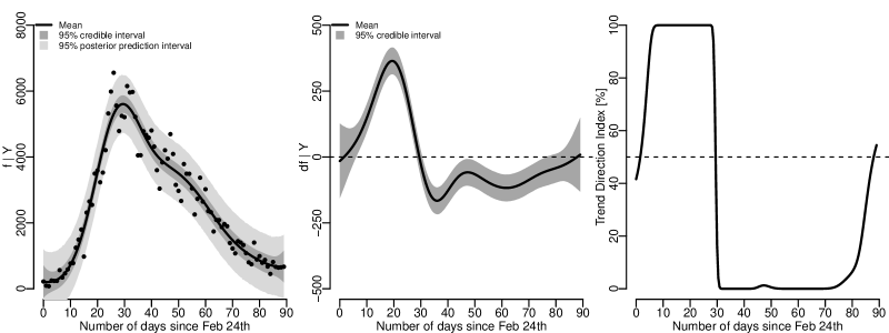
Figure 6: Results from the trend analysis of the Italian COVID-19 data. The left panel shows the number of new positives since February 24th along with the posterior mean of $f$ and 95% credible and posterior prediction intervals. The middle panel shows the posterior distribution of the trend ($df$), and the right panel shows the Trend Direction Index.

However, at day 88 (May 22nd, 2020) the Trend Direction Index had again increased and crossed 50%, and at the time of this analysis the index was equal to 54%. It is therefore currently not certain whether the number of new positives is increasing or decreasing but a slight probability favors the former. It should be stressed, that the Trend Direction Index monitors the sign and not the size of the trend and this recent increase of TDI to 54% may reflect that the number of new cases is merely starting to level off ($df(t)\approx 0$). The Trend Direction Index can be used as a monitoring tool to determine if the Italian authorities need to take extra actions.

6 Discussion

In this article we have proposed two new measures, the Trend Direction Index and the Expected Trend Instability, in order to quantify the trendiness of a latent, random function observed in discrete time. Using a Gaussian Process model for the latent structure we showed how these indices can be estimated from data in both a maximum likelihood and a Bayesian framework and provide probabilistic statements about the monotonicity of the latent development of an observed outcome over time.

Both indices have intuitive interpretations that directly refer to properties of the latent trend, and our proposed methodology exploits the assumption of continuity allowing us to calculate a different (and in many cases more relevant) probability than what can be obtained from e.g., multiple pairwise comparisons in discrete time.

The comparison with Trend Filtering showed that our proposed method provides unbiased estimates of the underlying function $f$ and its derivative, $df$ but that we are able to relax the assumptions of piece-wise linearity of the underlying process, while in addition providing a probability distribution for the derivative which is used directly in the Trend Direction Index and which directly provides the answers to the research questions often posed.

It is worth noting that the indices are scale-free and do not tell anything about the magnitude of a trend. Consequently, the two indices should therefore always be accompanied by plots of the posterior of $df$. If a prespecified magnitude, $u$, of a trend is desired, then the threshold in the definition of the TDI is easily modified to accommodate this as $\mathrm{TDI}_{u}(t,\delta)=P(df(t+\delta)>u\mid\mathcal{F}_{t})$.

In conclusion, we have introduced a method for quantifying the trendiness of a trend that specifically addresses questions such as “Has the trend changed?”. Our approach is based on two intuitive measures that are easily interpreted, provide well-defined measures of trend behavior, and which can be applied in a large number of situations. The flexibility of the model is further improved by the minimum of assumptions necessary to provide about the underlying latent trend.

Bibliography

Arnold, Taylor B., and Ryan J. Tibshirani. 2019. genlasso: Path Algorithm for Generalized Lasso Problems. https://CRAN.R-project.org/package=genlasso.

Barry, Daniel, and J. A. Hartigan. 1993. “A Bayesian Analysis for Change Point Problems.” Journal of the American Statistical Association 88 (421): 309–19.

Basseville, Michele, and Igor V. Nikiforov. 1993. Detection of Abrupt Changes: Theory and Application. Prentice-Hall.

Bergmeir, Christoph, and José M Benítez. 2012. “On the Use of Cross-Validation for Time Series Predictor Evaluation.” Information Sciences 191: 192–213.

Carlstein, Edward, Hans-Georg Müller, and David Siegmund, eds. 1994. Change-Point Problems. Vol. 23. Lecture Notes – Monograph Series. Institute of Mathematical Statistics.

Carpenter, Bob, Andrew Gelman, Matthew D Hoffman, Daniel Lee, Ben Goodrich, Michael Betancourt, Marcus Brubaker, Jiqiang Guo, Peter Li, and Allen Riddell. 2017. “Stan: A Probabilistic Programming Language.” Journal of Statistical Software 76 (1).

Chandler, R., and M. Scott. 2011. Statistical Methods for Trend Detection and Analysis in the Environmental Sciences. Statistics in Practice. Wiley.

Consiglio dei Ministri - Dipartimento della Protezione Civile, Presidenza del. 2020. “COVID-19 Italia - Monitoraggio Situazione.” 2020. https://github.com/pcm-dpc/COVID-19.

Cramer, Harald, and M. R. Leadbetter. 1967. Stationary and Related Stochastic Processes – Sample Function Properties and Their Applications. John Wiley & Sons, Inc.

Esterby, S. R. 1993. “Trend Analysis Methods for Environmental Data.” Environmetrics 4 (4): 459–81.

Gelman, Andrew, and Donald B. Rubin. 1992. “Inference from Iterative Simulation Using Multiple Sequences.” Statistical Science 7 (4): 457–72.

Gottlieb, Andrea, and Hans-Georg Müller. 2012. “A Stickiness Coefficient for Longitudinal Data.” Computational Statistics & Data Analysis 56 (12): 4000–4010.

Hodrick, Robert J., and Edward C. Prescott. 1997. “Postwar U.S. Business Cycles: An Empirical Investigation.” Journal of Money, Credit and Banking 29 (1): 1–16.

Jensen, Andreas Kryger. 2019. “GitHub Repository for the Trendiness of Trends.” 2019. https://github.com/aejensen/TrendinessOfTrends.

Kaufman, Cari G, Derek Bingham, Salman Habib, Katrin Heitmann, Joshua A Frieman, and others. 2011. “Efficient Emulators of Computer Experiments Using Compactly Supported Correlation Functions, with an Application to Cosmology.” The Annals of Applied Statistics 5 (4): 2470–92.

Kim, Seung-Jean, Kwangmoo Koh, Stephen Boyd, and Dimitry Gorinevsky. 2009. “$\ell_{1}$ Trend Filtering.” SIAM Review 51: 339–60.

Kowal, Daniel R., David S. Matteson, and David Ruppert. 2019. “Dynamic Shrinkage Processes.” Journal of the Royal Statistical Society: Series B 81: 781–804.

MacKay, D. J. C. 1998. “Introduction to Gaussian Process.” Neural Networks and Machine Learning.

Micchelli, Charles A, Yuesheng Xu, and Haizhang Zhang. 2006. “Universal Kernels.” Journal of Machine Learning Research 7 (Dec): 2651–67.

Navne, Helene, Anders Legarth Schmidt, and Lars Igum Rasmussen. 2019. “Første Gang I 20 år: Flere Danskere Ryger.” 2019. https://politiken.dk/forbrugogliv/sundhedogmotion/art6938627/Flere-danskere-ryger.

Neal, R. M. 2012. Bayesian Learning for Neural Networks. Lecture Notes in Statistics. Springer New York.

Quandt, Richard E. 1958. “The Estimation of the Parameters of a Linear Regression System Obeying Two Separate Regimes.” Journal of the American Statistical Association 53 (284): 873–80.

Radford, Neal M. 1999. “Regression and Classification Using Gaussian Process Priors (with Discussion).” In Bayesian Statistics 6: Proceedings of the Sixth Valencia International Meeting, edited by A. P. Dawid José M. Bernardo James O. Berger and Adrian F. M. Smith, 475–501.

Ramdas, Aaditya, and Ryan J. Tibshirani. 2016. “Fast and Flexible Admm Algorithms for Trend Filtering.” Journal of Computational and Graphical Statistics 25 (3): 839–58.

Rasmussen, C. E., and C. K. I. Williams. 2006. Gaussian Processes in Machine Learning. MIT Press.

R Core Team. 2018. R: A Language and Environment for Statistical Computing. Vienna, Austria: R Foundation for Statistical Computing. https://www.R-project.org/.

Stan Development Team. 2018. “RStan: The R Interface to Stan.” http://mc-stan.org/.

The Danish Health Authority. 2019. “Danskernes Rygevaner 2018.” 2019. www.sst.dk/da/udgivelser/2019/danskernes-rygevaner-2018.

Vehtari, Aki, Jonah Gabry, Mans Magnusson, Yuling Yao, and Andrew Gelman. 2019. “loo: Efficient Leave-One-Out Cross-Validation and WAIC for Bayesian Models.” https://mc-stan.org/loo.

Williams, Christopher KI. 1998. “Computation with Infinite Neural Networks.” Neural Computation 10 (5): 1203–16.