Efficient Video Semantic Segmentation with Labels Propagation and Refinement

Abstract

This paper tackles the problem of real-time semantic segmentation of high definition videos using a hybrid GPU-CPU approach. We propose an Efficient Video Segmentation (EVS) pipeline that combines:

(i) On the CPU, a very fast optical flow method, that is used to exploit the temporal aspect of the video and propagate semantic information from one frame to the next. It runs in parallel with the GPU.

(ii) On the GPU, two Convolutional Neural Networks: A main segmentation network that is used to predict dense semantic labels from scratch, and a Refiner that is designed to improve predictions from previous frames with the help of a fast Inconsistencies Attention Module (IAM). The latter can identify regions that cannot be propagated accurately.

We suggest several operating points depending on the desired frame rate and accuracy. Our pipeline achieves accuracy levels competitive to the existing real-time methods for semantic image segmentation (mIoU above 60%), while achieving much higher frame rates. On the popular Cityscapes dataset with high resolution frames ($2048\times 1024$), the proposed operating points range from 80 to 1000 Hz on a single GPU and CPU.

Keywords: Real-Time, Video Semantic Segmentation, Optical flow, Propagation, Refinement

1 Introduction

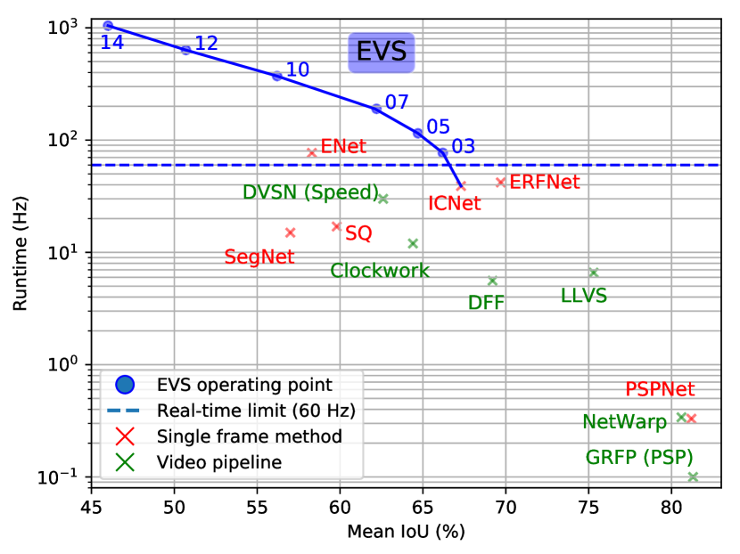
Figure 1: Comparison between our EVS pipeline and state of the art methods on the Cityscapes [8] dataset with input resolution $2048\times 1024$. Table 2 provides more operating points and comparisons, from 1 Hz to 1000 Hz.

A lot of efforts have been made in semantic segmentation over the past years. Yet, while segmentation accuracy reached astonishing levels, little focus has been put on making it usable in real-time scenarios. Achieving very fast semantic segmentation would have many advantages, especially when used as an additional building block for other computer vision tasks related to real-time scene understanding. Particularly in the context of real-world scenarios for industrial or commercial cases such as augmented reality, autonomous driving, autonomous flying, etc.

Video scene understanding is already a wide and active research topic, especially in accurate object instances tracking and segmentation. However, in the context of real-time video semantic segmentation, fewer efforts have been put into exploiting the temporal information as a mean to decrease inference time. When used, this temporal aspect is in most methods used as an additional information to improve either the accuracy of the predictions or their consistency over time, at the cost of additional runtime.

On the contrary, the focus of this paper is to use temporal information as a way to minimize the inference time for each frame as much as possible, while limiting the drop in accuracy resulting from the reduced computations. The baseline we use runs at around 40 Hz on a frame resolution of $2048\times 1024$. Our EVS pipeline defines several operating points among which the speedup factor varies from $\times 2$ to $\times 27$ on the same resolution.

The proposed pipeline uses ICNet [42] as the main prediction network, since it is the current state of the art in terms of trade-off between accuracy and performance for single frame processing. To compute the dense optical flow, we use Dense Inverse Search (DIS) [17] as it is the current state of the art in terms of computational efficiency on the CPU. Dense optical flow plays a key role in our pipeline, as it can run on the CPU in parallel with the GPU at a much higher frame rate than the prediction network. This information is then used to:

• Warp the semantic information from one frame to the next, both of high level predictions and low level contextual features. This warped semantics is used as input for the Refiner that will improve the labels prediction for the current frame.

• Feed the IAM to focus the refinement on regions where the optical flow is unreliable (typically thin and/or moving objects boundaries), by computing the forward-backward consistency of the propagated labels.

1.1 Contributions

Since semantic segmentation is crucial for video scene understanding, we aim at pushing the limits of this field through the following contributions, with a focus on efficiency and frame rate.

First, our hybrid EVS pipeline balances the workload between GPU and CPU. They work in parallel, either computing semantic predictions or propagating them from frame to frame using optical flow, instead of having one large pipeline running fully on the GPU. Running the optical flow directly on the CPU decreases the workload on the GPU and leads to a massive reduction in computation time. Our goal is to establish new standards in terms of speed for real-time video semantic segmentation while preserving a sound segmentation quality.

Furthermore, we introduce a fast IAM and a Refiner that work together to refine the propagated predictions of the main segmentation network to better match the current frame. Our versatile design allows running our pipeline in various operating modes, trading-off speed versus segmentation quality.

2 Related Work

The most straightforward way to perform video semantic segmentation is to simply run image semantic segmentation on each frame. Although this approach is rather slow, it leads to a natural baseline to assess the quality of video segmentation methods. Furthermore, we review recent trends and ideas in video segmentation. As our proposed method combines semantic image segmentation with optical flow, we review different methods extracting optical flow between consecutive frames using traditional or deep learning-based methods.

2.1 Image Semantic Segmentation

Semantic image segmentation aims at assigning a class label to each pixel of a given image. The recent advances in deep learning [16, 39] lead to fast progress in semantic image segmentation [23, 22, 5]. Most of the state-of-the-art methods [6, 43] are based on Fully Convolutional Networks (FCNs) [23]. Among these methods are: DeepLabV3+ [6], PSPNet [43] or more recently Panoptic FPN [15]. These methods concentrate mainly on high quality segmentation masks that require a large amount of parameters and are computationally intensive, i.e. inference time of around one second for a high resolution frame ($2048\times 1024$).

Other methods that focus on reducing computing time and memory footprint obtain more and more attention: SegNet [1], SQ [38], ENet [29] and ESPNet [26].

Combining the best of both worlds, some methods aim at finding good trade-offs between frame rate and accuracy, either from their model (ERFNet [32] and ICNet [42]) or by treating differently complex and simple parts of the image (LC [20]). These methods achieve faster inference times while preserving a decent segmentation quality.

2.2 Video Semantic Segmentation

Compared to semantic image segmentation, developing dedicated video segmentation pipelines is a less explored research track. Applying image segmentation algorithms that operate on each video frame individually is possible. However, specialized methods for videos can exploit temporal information between consecutive frames to enable more reliable predictions or increase the frame rate.

Early methods tackling video segmentation were extending classical single image segmentation methods with temporally-aware components: normalized cuts [35], tracking [19] or motion segmentation [28]. Recent methods leverage dense optical flow in a more direct way by combining it with Gated Recurrent Units (GRUs) to refine the predictions and add temporal consistency [37, 27].

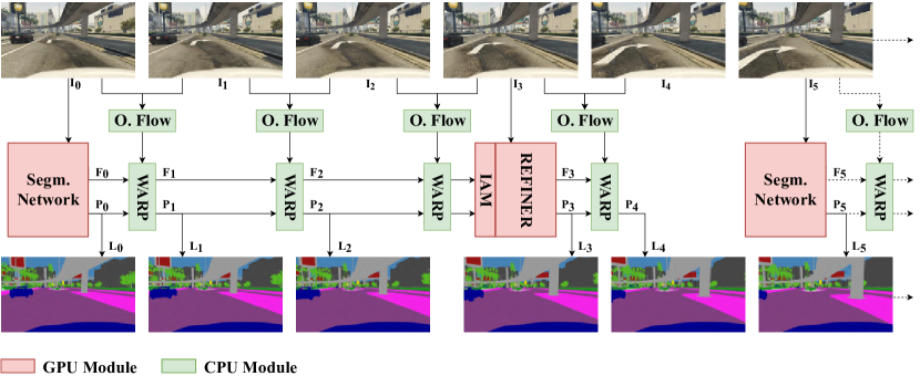
Figure 2: Full pipeline overview with an input video stream $(\boldsymbol{I_{0},I_{1},...})$ and the corresponding output labels $(\boldsymbol{L_{0},L_{1},...})$. The predicted probabilities $\boldsymbol{P_{i}}$, labels $\boldsymbol{L_{i}}$ and deep features $\boldsymbol{F_{i}}$ are propagated with the corresponding dense optical flow.

In particular, some methods aim at reducing inference times by embedding the temporal aspect in their structure by using LSTM [25], or by selecting key frames to fully segment. Clockwork [34] authors observe that intermediate representations within a network change only slowly in most videos. Therefore, they propose to schedule features computation for key frames only and share features in between. LLVS [21] and DVSN [41] try to further optimize scheduling depending on frame content.

Another family of methods uses the geometrical structure of the 3D scene to improve the segmentation quality. There, 3D point clouds obtained from visual odometry or stereo-vision approaches add additional information that allows more reliable predictions [3, 11, 33, 18].

One of the major challenges in video segmentation remains the massive amount of data that deep Convolutional Neural Networks (CNNs) require for training. Already, producing annotations for semantic image segmentation is costly. In this case, ensuring diversity in a video segmentation data set demands many different video sequences each consisting of hundreds of frames even for very short movies, leading to thousands of frames that should be annotated. Thus, existing data sets for video segmentation are either sparsely annotated [2, 13, 8], i.e. not every frame is labelled, or the segmentation task is simplified such that annotation is cheaper, i.e. single object segmentation [30]. In our case, we avoid this pitfall by relying on a network which is trained on single images. Only synthetic data sets such as GTA5 [31] or Sintel [4] overcome that annotation limitation.

2.3 Optical Flow

Traditional optical flow methods such as Lucas-Kanade [24] or Gunnar-Farneback [10], recently started to compete with new deep learning approaches: FlowNet [9, 14], MPNet [36] and SegFlow [7] produce very accurate flow estimates, but are rather expensive and slow and run on the GPU. As a result, deep video semantic segmentation pipelines using optical flow usually improve marginally their accuracy or temporal consistency, while increasing substantially their inference time: NetWarp [12], GRFP [27] or DFF [40]. In contrast, when aiming at fast and efficient video segmentation, DIS [17] is among the most suitable candidates. DIS achieves much higher frame rates than deep optical flow methods and runs on CPU, which gives more flexibility to choose between speed and accuracy by selecting different operating points.

3 Efficient Video Segmentation Pipeline

3.1 Full Pipeline Overview

Our pipeline consists of five main components that process the video stream jointly, see Figure  2. The GPU holds a segmentation network and a Refiner with IAM, while the CPU is responsible for computing in parallel the optical flow and for warping the CNN features and predictions.

The dense optical flow is computed for each pair of the consecutive frames. It enables the forward and backward remapping of semantic information extracted by the deep networks. The IAM is responsible for computing the inconsistencies that remapping reveals. It provides this information to the Refiner, which then corrects mistakes caused by warping around inconsistent areas, i.e. where the optical flow is not reliable.

In the best case, the flow will be consistent and the prediction of the next frame will simply be the previous prediction warped by using optical flow. In most cases, the lack of flow consistency in some regions of the image (sudden changes in brightness, occlusions, multiple fast motions, etc.) will be recovered by the Refiner, while the other prediction of other regions will still be derived from the previous prediction to increase temporal consistency.

3.2 Semantic Segmentation Network

The segmentation network in our pipeline is responsible for providing a full frame semantic segmentation. We want to emphasize that any deep framework can be used within our framework, leaving space for improvements when better networks are developed. For this work, we choose to use ICNet [42] because of its excellent trade-off between accuracy and speed: 67% mIoU at $\sim 40$ Hz on the popular Cityscapes [8] dataset.

3.3 Optical Flow and Semantics Propagation

The advent of deep learning brought many optical flow methods to impressive quality levels while focusing less on the computational efficiency. However, we require a fast but still accurate dense optical flow. DIS Flow [17] matches perfectly this requirement and has the advantage of producing a reasonable dense flow at a very high frame rate while running on the CPU. Thus, it allows to save the GPU resources for other tasks.

Dense optical flow provides for each pixel $(x,y)$ of the image a flow in each dimension $F_{xy}^{1\rightarrow 2}(x,y)$, between two consecutive frames $I_{1}$ and $I_{2}$. The mapping between $I_{1}$ and $I_{2}$ can be written for each dimension as follows:

$$\begin{split}M_{x}(x,y)=I_{2}(x,y)-F_{x}^{1\rightarrow 2}(x,y)\\ M_{y}(x,y)=I_{2}(x,y)-F_{y}^{1\rightarrow 2}(x,y)\end{split}$$ (1)

Using Eq. (1) then allows to produce image $I_{2}$ solely by remapping the pixels from image $I_{1}$. For non-integer valued coordinates, using the nearest neighbours interpolation results in a valid remapped image:

$$I_{2}(x,y)=I_{1}(M_{x}(x,y),M_{y}(x,y))$$ (2)

We want to emphasize that such a mapping is fast to perform because it is highly parallelizable on CPU. In our pipeline, it is used to quickly remap both the predictions and the low level CNN features from one frame to the next. These features represent the slow changing contextual information of the scene. The predictions can also be remapped backward such that the IAM is able to compute the inconsistencies (Figure 3).

3.4 Inconsistencies Attention Module

The IAM is working together with the Refiner. It is designed such that it is lightweight and able to focus the attention of the refinement on regions where the optical flow is inconsistent. The inputs are:

• $L_{\textrm{F}}$: the labels predicted for the current frame, obtained by warping the previous frame labels forward.

• $L_{\textrm{BF}}$: the labels predicted for the current frame, obtained by warping the labels backward and then forward $L_{F}$.

• $P_{\textrm{refiner}}$: the predicted probabilities for each class by the Refiner.

• $P_{\textrm{warped}}$: the predicted probabilities warped using the optical flow.

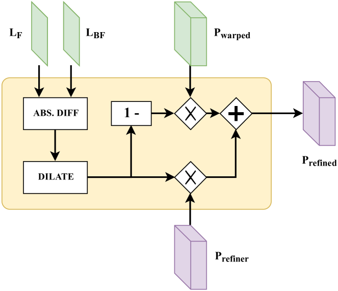
Figure 3: Inconsistencies Attention Module.

As a first step, the module computes a probability map $M_{i}$ that represents the forward-backward inconsistencies of the optical flow for the given input frames. For every pixel $(m,n)$ where $L_{\textrm{F}}$ and $L_{\textrm{BF}}$ are different, the probability is considered to be maximal because the flow is unreliable. All other pixels are considered to be reliable:

$$M_{i}(m,n)=\begin{cases}1.0&\text{if $L_{\textrm{F}}(m,n)\neq L_{\textrm{BF}}(m,n)$}\\ 0.0&\text{otherwise}\end{cases}$$ (3)

As a second step, this binary mask is dilated and smoothed to engulf the surrounding areas of the inconsistencies and to let the Refiner act on them, as the predictions in these regions are more likely to be wrongly propagated by the optical flow.

Finally, the predicted probabilities for each pixel are weighted differently between the warped prediction and the prediction of the Refiner. If $P_{\textrm{refiner}}$ is the prediction of the Refiner and $P_{\textrm{warped}}$ is the previous prediction warped to the current frame using the optical flow, the final refined prediction $P_{\textrm{refined}}$ is defined as the sum of the Hadamard products:

$$P_{\textrm{refined}}=M_{i}\circ P_{\textrm{refiner}}+(1-M_{i})\circ P_{\textrm{warped}}$$ (4)

As shown in Figure 3, the module only consists of lightweight operations for a GPU, especially since the inputs and outputs are processed at a resolution of $512\times 256$.

3.5 Refiner

A carefully performed benchmark of the branches in the ICNet architecture shows that even though the network is designed to limit the heavy computations on the lowest resolution to limit the inference time per frame, almost half of that time is spent only on building low level features (see Figure 5). The Refiner is built on the idea that these low level features do not need to be recomputed every frame in the context of a continuous video stream: due to their resolution, they are changing at the slowest rate over time.

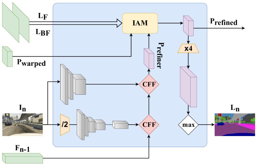
Figure 4: Refiner architecture. For a given input image $\boldsymbol{I_{n}}$ and warped semantics from the previous frames (green), it generates refined probabilities $\boldsymbol{P_{\textrm{refined}}}$ and labels $\boldsymbol{L_{n}}$. CFF stands for ”Cascade Feature Fusion”, as in ICNet [42].

Its task is different from the segmentation network: given pre-aligned low level features from past frames, the Refiner should only compute the higher level features for the new frame, making it shallower. This allows sparing half of the computations that would then otherwise be carried out to extract low level features.

Besides, with the help of the IAM, this refinement is focused only on some areas of the image (see Figure 4). Using the dense optical flow is reliable for large portions of the image but it causes errors next to object boundaries especially when these objects are thin, moving or new. Thus, using the IAM leads to a better temporal consistency overall, as most of the predicted labels were propagated from one frame to the next.

4 Experimental evaluation

4.1 Setup and Benchmarking Method

All the benchmarks are done using a single Nvidia Titan Xp GPU, and a Intel Core i7-5930K CPU @ 3.50GHz. The implementation is different from the original ICNet implementation which is written in Caffe and uses a proprietary version of ResNet50. Instead, we use an equivalent implementation in Tensorflow 1.8 and CUDNN 7.1 as the baseline for this paper. The Tensorflow implementation yields almost the same performance and accuracy (67.3% vs. 67.7%). All the benchmarks and comparisons in this paper use this Tensorflow implementation. It is worth noting that this is not problematic because the segmentation network of our pipeline can be replaced by any other implementation.

All the following benchmarks and results are produced on Cityscapes [8], which contains short video snippets of 30 frames at a high resolution ($2048\times 1024$) among which the 20 frame contains a fully annotated ground truth mask. All the experiments and results presented are evaluated on the 20 frame with different starting points before it depending on the operating points.

For us, it is important to measure the computation times on the GPU as accurately as possible. Thus, we build a specific probe class based on the publicly available Tensorflow Profiler, which provides the detailed timestamps for each operation on the GPU in JSON format. This data allows us to establish very accurate timings for each part of the network.

Each measurement contains 300 samples from the extracted profiler data. In order to avoid border effects, we measure each sample in middle of the execution of the network. The measurements show that the timings are more varied at the startup time and the initialization of the models. Nonetheless, following the aforementioned strategy leads to reliable and accurate GPU computation times: the average and median measurements are matching with a small standard deviation, see Figure 5.

4.2 Runtime of the different components

On the CPU side, warping pixels from one frame to the next using optical flow can be easily parallelized on the CPU. Once split in a $3\times 3$ or $4\times 4$ grid, all the pixels from a full frame are remapped within a marginal time period ($\sim 0.15$ ms on a Intel Core i7-5930K CPU @ 3.50GHz).

On the GPU side, we have two models: one for the full CNN and the other for the Refiner. ICNet [42] is structured around 3 branches: Branch1 with very few convolutions operating at full resolution, Branch2 that computes deep features starting from half the resolution, and Branch4 that goes much deeper at even lower resolution. Figure 5 shows a speedup of almost two times for the inference time of the Refiner.

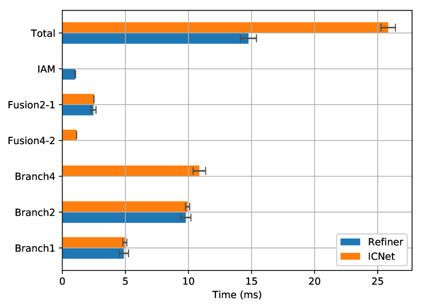
Figure 5: Runtime of the Refiner with IAM compared to ICNet on a single Nvidia Titan Xp.

4.3 Optical Flow and Labels Propagation

4.3.1 Optical Flow Benchmark

Several operating points are suggested for DIS [17], with a set of parameters that trade off accuracy and runtime. For our experiments, we choose a set of parameters to achieve a small runtime: no variational refinement, finest scale $\theta_{f}=2$, patch size $\theta_{ps}=8$, gradient descent iterations $\theta_{it}=12$. This allows us to run the optical flow computation on one of the cores of the CPU, on the full frame resolution $2048\times 1024$ in less than 5 ms. The goal is to compute the optical flow for five frames on one core, while the segmentation network is working ($\sim 25$ ms, see Figure 5).

4.3.2 Influence of the Optical Flow Algorithm

The dense optical flow computation is of paramount importance to propagate the semantic information correctly. Figure 6 shows the comparison between DIS [17] at a fast operating point and Gunnar-Farneback [10] with a 2 layers pyramid, an averaging window of 9 pixels and 15 iterations. There is a substantial difference in the mIoU already after the first propagation.

Experiments with higher quality settings for DIS [17] showed marginal improvements (below 0.2%) on the mIoU even at high resolution, which motivated our choice for a faster operating point. With the ultra fast setting, the drop per propagation on the highest resolution is between 1.0% and 1.5% (1.2% on average). This drop also tends to decrease when the resolution decreases, which is particularly interesting for the predictions and low level forward propagation of the features, since they operate at a resolution of $512\times 256$ and $128\times 64$ respectively.

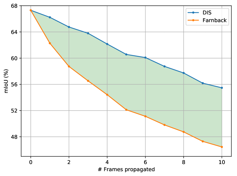
Figure 6: Influence of a pure label propagation on the mIoU for $2048\times 1024$, comparison Gunnar-Farnebäck vs. DIS.

4.3.3 Uncertainties across the Evaluation Set

The inconsistencies detected by forward-backward warping of the labels with the optical flow vary depending on the frame content and increase globally after each propagation. Figure 7 shows on the evaluation set of CityScapes [8] how the uncertainties are distributed depending on the number of propagations. This shows that even after 4 propagations, less than 5% of the flow computed is detected as inconsistent on average. For frame-to-frame propagation, this drops to less than 1%, which confirms that the optical flow is highly consistent.

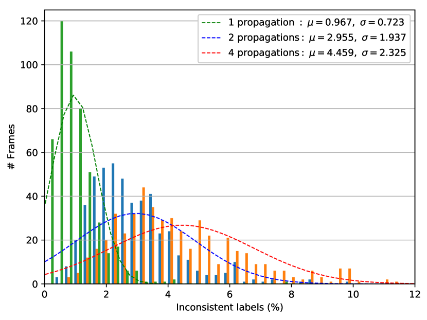
Figure 7: Re-partition of frames on the Cityscapes [8] evaluation set as a function of their percentage of forward-backward inconsistent pixels from the optical flow, after 1, 2 and 4 propagations.

Method	Total	road	swalk	build.	wall	fence	pole	tlight	sign	veg.	terrain	sky	person	rider	car	truck	bus	train	mbike	bike
Baseline	67.3	97.4	79.5	89.4	49.1	51.7	46.1	47.9	61.1	90.3	58.6	93.4	69.9	43.3	91.4	64.8	75.8	59.9	43.9	65.4
EVS 03	66.2	97.3	78.9	89.1	51.1	52.1	41.5	46.6	60.4	89.8	59.2	93.1	66.9	41.7	90.5	64.1	75.2	52.1	44.5	64.2
EVS 02	66.8	97.3	79.1	89.3	51.0	52.3	44.5	47.1	61.4	90.2	59.5	93.2	69.0	42.5	90.9	63.9	75.5	52.5	45.0	64.9
Recovery	+0.6$\color[rgb]{0,1,0}\bigtriangleup$	=	+0.2	+0.2	-0.1	+0.2	+3.0	+0.5	+1.0	+0.4	+0.3	+0.1	+2.1	+0.8	+0.4	-0.2	+0.3	+0.4	+0.5	+0.7
EVS 07	62.2	96.8	77.1	87.4	50.6	49.5	31.3	43.5	55.5	87.9	55.9	92.6	57.9	35.4	87.2	59.8	72.0	41.8	40.3	58.5
EVS 06	63.0	96.6	75.6	87.9	50.2	49.8	36.0	44.4	57.5	89.1	56.6	93.2	63.6	36.5	87.5	59.2	70.8	41.5	41.1	60.0
Recovery	+0.8$\color[rgb]{0,1,0}\bigtriangleup$	-0.2	-1.5	+0.5	-0.4	+0.3	+4.7	+0.9	+2.0	+1.2	+0.7	+0.6	+5.7	+1.1	+0.3	-0.6	-1.2	-0.3	+0.8	+1.5

Table 1: Per-class results on Cityscapes after propagating 1 or 4 times the labels with refinement (EVS 02 and EVS 06) or without (EVS 03 and EVS 07). The corresponding recovery achieved by the Refiner is explicitely mentioned for both cases.

4.4 EVS Operating Points

4.4.1 Per Class Impact of Warping and Refinement

As discussed before, a simple forward mapping of the predictions made by the segmentation network can bring an important speedup factor, at a cost of an overall marginally degraded segmentation quality. Although the drop in mIoU per propagation might seem marginal, it is directly correlated to the mistakes of the optical flow (especially around boundaries of moving objects, thin objects and occlusions that may happen over time) and might have a big impact locally.

A per class analysis (see Table 1) confirms that the errors due to optical flow propagation affect most classes only marginally (below 1% drop in IoU). Some of them are particularly affected by the wrong labeling: static thin objects (poles, traffic signs, traffic lights) and humans/small moving objects (person, rider, bike) are the most impacted classes (between 1% and 5% drop in IoU).

The Refiner is able to recover a large portion of the drop in IoU observed for those classes, especially after 1 frame propagation for poles, street signs and persons, even though the overall IoU gain is between 0.5% and 1%. Figure 8 shows these typical situations where the refinement has a clear visible impact on these specific classes and shows that our Refiner can recover missing parts:

• Thin objects such as poles, street signs or traffic lights are not always captured or heavily distorted by the camera motion.

• Pedestrians on a crossing or cyclists and bikes are sometimes difficult to be fully captured with optical flow.

• Missing parts due to occlusion and moving objects: a cyclist and bike passing in front of vegetation or two cars at a crossing.

Interestingly, the analysis also reveals that large static classes benefit from propagation (wall, fence, terrain) such that the IoU for these classes is higher than the IoU produced by the baseline, even without refinement (between 0.5% and 2% gain in IoU).

4.4.2 Operating Point Comparison

The structure of our EVS pipeline is defined by four parameters: the downscaling factor used by the segmentation network (D), the rate (every $n^{th}$ frame) at which the full segmentation is computed (S), warping (W) and refinement (R). Table 2 summarizes these operating points and compares them with state-of-the-art methods in terms of accuracy, frame rate and speedup factor compared to our baseline ICNet [42].

	Method	Framerate	Speedup	D	S	W	R	mIoU
Video pipeline	EVS 14 (Ours)	1045 Hz	$\times 27.1$	0.5	17	✓	✗	46.0%
	EVS 13 (Ours)	677 Hz	$\times 17.6$	0.5	10	✗	✗	35.3%
	EVS 12 (Ours)	634 Hz	$\times 16.5$	0.5	10	✓	✗	50.7%
	EVS 11 (Ours)	387 Hz	$\times 10.1$	1.0	10	✗	✗	36.7%
	EVS 10 (Ours)	372 Hz	$\times 9.7$	1.0	10	✓	✗	56.2%
	EVS 09 (Ours)	339 Hz	$\times 8.8$	0.5	5	✗	✗	42.8%
	EVS 08 (Ours)	192 Hz	$\times 5.0$	1.0	5	✗	✗	46.4%
	EVS 07 (Ours)	190 Hz	$\times 4.9$	1.0	5	✓	✗	62.2%
	EVS 06 (Ours)	122 Hz	$\times 3.2$	1.0	5	✓	✓	63.0%
	EVS 05 (Ours)	115 Hz	$\times 3.0$	1.0	3	✓	✗	64.7%
	EVS 04 (Ours)	74 Hz	$\times 1.9$	1.0	3	✓	✓	65.6%
	EVS 03 (Ours)	77 Hz	$\times 2.0$	1.0	2	✓	✗	66.2%
	EVS 02 (Ours)	49 Hz	$\times 1.2$	1.0	2	✓	✓	66.8%
	EVS 01 (Ours)	37 Hz	$\times 0.95$	1.0	1	✓	✓	67.6%
	DVSN [41]	30 Hz	$\times 0.8$	-	-	-	-	62.6%
	Clockwork [34]	12 Hz	$\times 0.3$	-	-	-	-	64.4%
	LLVS [21]	6.6 Hz	$\times 0.2$	-	-	-	-	75.3%
	DFF [40]	5.6 Hz	$\times 0.1$	-	-	-	-	69.2%
	GRFP [27]	0.6 Hz	$\times 0.02$	-	-	-	-	81.3%
	NetWarp [12]	0.3 Hz	$\times 0.01$	-	-	-	-	80.6%
Single frame	ENet [29]	77 Hz	$\times 1.9$	-	-	-	-	58.3%
	ERFNet [32]	42 Hz	$\times 1.1$	-	-	-	-	69.7%
	ICNet[42]	39 Hz	Ref.–	-	-	-	-	67.3%
	SQ [38]	17 Hz	$\times 0.4$	-	-	-	-	59.8%
	SegNet [1]	15 Hz	$\times 0.4$	-	-	-	-	57.0%
	PSPNet [43]	0.8 Hz	$\times 0.02$	-	-	-	-	81.2%

Table 2: Comparison of different EVS pipeline operating points. Numbers are reported on a Nvidia Titan Xp GPU and Intel Core i7-5930K CPU @3.50GHz for our pipeline and the reproduced ICNet [42]. Numbers for other methods are reported from their respective papers on various hardware.

(a) Ground truth

(b) ICNet

(c) EVS Propagated

(d) EVS Propagated + Refined

Figure 8: Benefits of the Refiner on the propagated predictions in three problematic situations for the optical flow: a person riding a bike, thin poles on the side walk and occlusions from cars.

5 Conclusion

In this work, we introduce an Efficient Video Segmentation pipeline that pushes the boundaries of real-time video semantic segmentation in terms of computational efficiency by combining the benefits of deep CNNs running on the GPU and a very fast optical flow running in parallel with the CPU. We propose different operating modes in order to focus either on frame rate or accuracy, from 67% mIoU at $\sim 40$ Hz to 46% mIoU at $\sim 1000$ Hz for $2048\times 1024$ input images.

To compensate for the introduced errors in the predictions by the optical flow propagation around thin and/or moving objects (poles, persons or bikes), we propose a Refiner network to correct some errors and to generate a visually more appealing segmentation. The Refiner works with a dedicated Inconsistencies Attention Module which focuses the prediction refinement on the relevant regions of the image.

One of the strengths of our pipeline is that the segmentation network can be used as a black box method and can be replaced with any other segmentation network, bringing potentially more accuracy for the same speedups in the future. Moreover, our pipeline could benefit from a higher input frame rate because two consecutive frames are more similar and lead to a more accurate and reliable optical flow prediction (Cityscapes has a rather small frame rate of 17 Hz). Furthermore, the IAM introduced in this paper could be used in a future work as a way to dynamically adapt the behaviour of our pipeline depending to the input frames. In simple situations, the segmentation network and the Refiner could run less often such that the whole pipeline relies more on the optical flow when it is reliable. In more complex situations, the pipeline would then be able to force the re-segmentation more often to preserve a reasonable accuracy at the price of a lower frame rate.

References

- [1] V. Badrinarayanan, A. Kendall, and R. Cipolla. Segnet: A deep convolutional encoder-decoder architecture for image segmentation. IEEE Transactions on Pattern Analysis and Machine Intelligence, 39:2481–2495, 2016.
- [2] G. J. Brostow, J. Fauqueur, and R. Cipolla. Semantic object classes in video: A high-definition ground truth database. Pattern Recognition Letters, 30:88–97, 2009.
- [3] G. J. Brostow, J. Shotton, J. Fauqueur, and R. Cipolla. Segmentation and recognition using structure from motion point clouds. In ECCV, 2008.
- [4] D. J. Butler, J. Wulff, G. B. Stanley, and M. J. Black. A naturalistic open source movie for optical flow evaluation. In A. Fitzgibbon et al. (Eds.), editor, European Conf. on Computer Vision (ECCV), Part IV, LNCS 7577, pages 611–625. Springer-Verlag, Oct. 2012.
- [5] L. Chen, G. Papandreou, I. Kokkinos, K. Murphy, and A. L. Yuille. Deeplab: Semantic image segmentation with deep convolutional nets, atrous convolution, and fully connected crfs. IEEE Trans. Pattern Anal. Mach. Intell., 40(4):834–848, 2018.
- [6] L.-C. Chen, Y. Zhu, G. Papandreou, F. Schroff, and H. Adam. Encoder-decoder with atrous separable convolution for semantic image segmentation. In The European Conference on Computer Vision (ECCV), September 2018.
- [7] J. Cheng, Y.-H. Tsai, S. Wang, and M.-H. Yang. Segflow: Joint learning for video object segmentation and optical flow. In IEEE International Conference on Computer Vision (ICCV), 2017.
- [8] M. Cordts, M. Omran, S. Ramos, T. Rehfeld, M. Enzweiler, R. Benenson, U. Franke, S. Roth, and B. Schiele. The cityscapes dataset for semantic urban scene understanding. In Proc. of the IEEE Conference on Computer Vision and Pattern Recognition (CVPR), 2016.
- [9] A. Dosovitskiy, P. Fischer, E. Ilg, P. Häusser, C. Hazırbaş, V. Golkov, P. v.d. Smagt, D. Cremers, and T. Brox. Flownet: Learning optical flow with convolutional networks. In IEEE International Conference on Computer Vision (ICCV), 2015.
- [10] G. Farnebäck. Two-frame motion estimation based on polynomial expansion. In J. Bigün and T. Gustavsson, editors, Image Analysis, 13th Scandinavian Conference, SCIA 2003, Halmstad, Sweden, June 29 - July 2, 2003, Proceedings, volume 2749 of Lecture Notes in Computer Science, pages 363–370. Springer, 2003.
- [11] G. Floros and B. Leibe. Joint 2d-3d temporally consistent semantic segmentation of street scenes. 06 2012.
- [12] R. Gadde, V. Jampani, and P. V. Gehler. Semantic video cnns through representation warping. In IEEE International Conference on Computer Vision (ICCV). IEEE, 2017.
- [13] A. Geiger, P. Lenz, C. Stiller, and R. Urtasun. Vision meets robotics: The kitti dataset. International Journal of Robotics Research (IJRR), 2013.
- [14] E. Ilg, N. Mayer, T. Saikia, M. Keuper, A. Dosovitskiy, and T. Brox. Flownet 2.0: Evolution of optical flow estimation with deep networks. In IEEE Conference on Computer Vision and Pattern Recognition (CVPR), 2017.
- [15] A. Kirillov, R. B. Girshick, K. He, and P. Dollár. Panoptic feature pyramid networks. CoRR, abs/1901.02446, 2019.
- [16] A. Krizhevsky, I. Sutskever, and G. E. Hinton. Imagenet classification with deep convolutional neural networks. In Proceedings of the 25th International Conference on Neural Information Processing Systems - Volume 1, NIPS’12, pages 1097–1105, USA, 2012. Curran Associates Inc.
- [17] T. Kroeger, R. Timofte, D. Dai, and L. V. Gool. Fast optical flow using dense inverse search. In Proceedings of the European Conference on Computer Vision (ECCV), 2016.
- [18] A. Kundu, Y. Li, F. Dellaert, F. Li, and J. M. Rehg. Joint semantic segmentation and 3d reconstruction from monocular video. In D. Fleet, T. Pajdla, B. Schiele, and T. Tuytelaars, editors, Computer Vision – ECCV 2014, pages 703–718, Cham, 2014. Springer International Publishing.
- [19] J. Lezama, K. Alahari, J. Sivic, and I. Laptev. Track to the future: Spatio-temporal video segmentation with long-range motion cues. In IEEE Conference on Computer Vision and Pattern Recognition, 2011.
- [20] X. Li, Z. Liu, P. Luo, C. Change Loy, and X. Tang. Not all pixels are equal: Difficulty-aware semantic segmentation via deep layer cascade. In The IEEE Conference on Computer Vision and Pattern Recognition (CVPR), July 2017.
- [21] Y. Li, J. Shi, and D. Lin. Low-latency video semantic segmentation. In The IEEE Conference on Computer Vision and Pattern Recognition (CVPR), June 2018.
- [22] Z. Liu, X. Li, P. Luo, C. C. Loy, and X. Tang. Semantic image segmentation via deep parsing network. 2015 IEEE International Conference on Computer Vision (ICCV), pages 1377–1385, 2015.
- [23] J. Long, E. Shelhamer, and T. Darrell. Fully convolutional networks for semantic segmentation. In IEEE Conference on Computer Vision and Pattern Recognition, CVPR 2015, Boston, MA, USA, June 7-12, 2015, pages 3431–3440. IEEE Computer Society, 2015.
- [24] B. D. Lucas and T. Kanade. Optical navigation by the method of differences. In A. K. Joshi, editor, Proceedings of the 9th International Joint Conference on Artificial Intelligence. Los Angeles, CA, USA, August 1985, pages 981–984. Morgan Kaufmann, 1985.
- [25] B. Mahasseni, S. Todorovic, and A. Fern. Budget-aware deep semantic video segmentation. 2017 IEEE Conference on Computer Vision and Pattern Recognition (CVPR), pages 2077–2086, 2017.
- [26] S. Mehta, M. Rastegari, A. Caspi, L. Shapiro, and H. Hajishirzi. Espnet: Efficient spatial pyramid of dilated convolutions for semantic segmentation. In The European Conference on Computer Vision (ECCV), September 2018.
- [27] D. Nilsson and C. Sminchisescu. Semantic video segmentation by gated recurrent flow propagation. In The IEEE Conference on Computer Vision and Pattern Recognition (CVPR), June 2018.
- [28] P. Ochs, J. Malik, and T. Brox. Segmentation of moving objects by long term video analysis. IEEE Trans. Pattern Anal. Mach. Intell., 36(6):1187–1200, June 2014.
- [29] A. Paszke, A. Chaurasia, S. Kim, and E. Culurciello. Enet: A deep neural network architecture for real-time semantic segmentation. CoRR, abs/1606.02147, 2016.
- [30] F. Perazzi, J. Pont-Tuset, B. McWilliams, L. Van Gool, M. Gross, and A. Sorkine-Hornung. A benchmark dataset and evaluation methodology for video object segmentation. In Computer Vision and Pattern Recognition, 2016.
- [31] S. R. Richter, V. Vineet, S. Roth, and V. Koltun. Playing for data: Ground truth from computer games. In B. Leibe, J. Matas, N. Sebe, and M. Welling, editors, European Conference on Computer Vision (ECCV), volume 9906 of LNCS, pages 102–118. Springer International Publishing, 2016.
- [32] E. Romera, J. M. Alvarez, L. M. Bergasa, and R. Arroyo. Erfnet: Efficient residual factorized convnet for real-time semantic segmentation. IEEE Transactions on Intelligent Transportation Systems, 19:263–272, 2018.
- [33] S. Sengupta, E. Greveson, A. Shahrokni, and P. H. S. Torr. Urban 3d semantic modelling using stereo vision. 2013 IEEE International Conference on Robotics and Automation, pages 580–585, 2013.
- [34] E. Shelhamer, K. Rakelly, J. Hoffman, and T. Darrell. Clockwork convnets for video semantic segmentation. In G. Hua and H. Jégou, editors, Computer Vision – ECCV 2016 Workshops, pages 852–868, Cham, 2016. Springer International Publishing.
- [35] J. Shi and J. Malik. Normalized cuts and image segmentation. IEEE Trans. Pattern Anal. Mach. Intell., 22(8):888–905, Aug. 2000.
- [36] P. Tokmakov, K. Alahari, and C. Schmid. Learning motion patterns in videos. In CVPR, 2017.
- [37] P. Tokmakov, K. Alahari, and C. Schmid. Learning Video Object Segmentation with Visual Memory. In ICCV - IEEE International Conference on Computer Vision, pages 4491–4500, Venice, Italy, Oct. 2017. IEEE.
- [38] M. Treml, J. A. Arjona-Medina, T. Unterthiner, R. Durgesh, F. Friedmann, P. Schuberth, A. Mayr, M. Heusel, M. Hofmarcher, M. Widrich, B. Nessler, and S. Hochreiter. Speeding up semantic segmentation for autonomous driving. In NIPS workshop, 2016.
- [39] Z. Wu, C. Shen, and A. van den Hengel. Wider or deeper: Revisiting the resnet model for visual recognition. CoRR, abs/1611.10080, 2016.
- [40] J. D. L. Y. Y. W. Xizhou Zhu, Yuwen Xiong. Deep feature flow for video recognition. 2017.
- [41] Y.-S. Xu, T.-J. Fu, H.-K. Yang, and C.-Y. Lee. Dynamic video segmentation network. In The IEEE Conference on Computer Vision and Pattern Recognition (CVPR), June 2018.
- [42] H. Zhao, X. Qi, X. Shen, J. Shi, and J. Jia. Icnet for real-time semantic segmentation on high-resolution images. In The European Conference on Computer Vision (ECCV), September 2018.
- [43] H. Zhao, J. Shi, X. Qi, X. Wang, and J. Jia. Pyramid scene parsing network. In The IEEE Conference on Computer Vision and Pattern Recognition (CVPR), July 2017.