A Multi-Site Stochastic Weather Generator for High-Frequency Precipitation Using Censored Skew-Symmetric Distribution

Abstract

Stochastic weather generators (SWGs) are digital twins of complex weather processes and widely used in agriculture and urban design. Due to improved measuring instruments, an accurate SWG for high-frequency precipitation is now possible. However, high-frequency precipitation data are more zero-inflated, skewed, and heavy-tailed than common (hourly or daily) precipitation data. Therefore, classical methods that either model precipitation occurrence independently of their intensity or assume that the precipitation follows a censored meta-Gaussian process may not be appropriate. In this work, we propose a novel multi-site precipitation generator that drives both occurrence and intensity by a censored non-Gaussian vector autoregression model with skew-symmetric dynamics. The proposed SWG is advantageous in modeling skewed and heavy-tailed data with direct physical and statistical interpretations. We apply the proposed model to 30-second precipitation based on the data obtained from a dense gauge network in Lausanne, Switzerland. In addition to reproducing the high-frequency precipitation, the model can provide accurate predictions as the long short-term memory (LSTM) network but with uncertainties and more interpretable results.

Keywords: Censored data, digital twins, non-Gaussian processes, skewed distribution, spatio-temporal model

1 Introduction

Tremendous efforts have been made to model, forecast, and reproduce local and global precipitation patterns. Among these efforts, the stochastic weather generator (SWG) makes use of statistical tools to simulate random sequences and reproduce atmospherical variables efficiently (Wilks and Wilby,, 1999). Typically, an ideal stochastic precipitation generator (SPG) should be able to reproduce the statistical properties of occurrence, intensity, and dry spell length of precipitation. The idea of reproducing physical processes with a virtual replica applied in other areas, such as “digital twin” (Boschert and Rosen,, 2016; Söderberg et al.,, 2017; El Saddik,, 2018). A Digital twin integrates many modern techniques such as internet of things and artificial intelligence. It is also the critical sector of smart city (Falconer and Mitchell,, 2012) and industry 4.0 (Gilchrist,, 2016).

SPGs have proven to be important in water resources research. As an example of digital twins, SPGs provide valuable information for water resource management for a smart city (Parra et al.,, 2015). In hydrologic and agricultural science, SPGs can serve as an input in further simulations of erosion, flood and crop growth (Mary et al.,, 2009). Moreover, as the primary atmospheric variable in SWGs, precipitation is typically used to generate other variables, such as wind and solar irradiance, due to their close association with rainfall occurrence (Richardson,, 1981). Techniques in modeling precipitation data can be also beneficial to other fields of study, such as sociology (Heckman,, 1976) and economics (McDonald and Moffitt,, 1980), where the data properties are often similar to those of precipitation, e.g., they are zero-inflated, nonnegative, right-skewed, heavy-tailed, and correlated in space and time.

Due to their wide applicability and the intriguing challenges, studies of SPGs have drawn attentions since 1960s (Gabriel and Neumann,, 1962) and been systematic reviewed in Wilks and Wilby, (1999), Srikanthan and McMahon, (2001), and Ailliot et al., (2015). Traditional studies mainly focus on the SPGs with a low temporal resolution, usually on a daily scale, due to the data available. For instance, the most popular chain-dependent model (Katz,, 1977; Richardson,, 1981) assumes that the occurrence processes can be modeled independently of intensity by Markov chains, and the intensity processes can be estimated conditionally on wet events using Gamma or exponential distributions. However, their assumption of independent occurrence is not appropriate for high-frequency precipitation, since greater quantities of rainfall in the past may lead to a significantly higher probability of occurrence (Koch and Naveau,, 2015).

Recently, acoustic rain gauges are able to provide precise and high-frequency data which are undetectable by the classical measurement devices, such as tipping-bucket rain gauge, satellite-based radar, and terrestrial radar. The high-frequency dataset is valuable to many rainfall-related phenomena, such as rapid surface water runoff, flash flooding, and small river catchments (Chan et al.,, 2016). However, the rainfall model at this scale has been rarely developed and assessed. To our knowledge, only Benoit et al., (2018) has performed an investigation of the minutely and sub-kilometer SPGs with the same device; in their study, the spatial dependence was the major concern. Even though broad literatures exist on the development of hourly and daily SPGs, we cannot assume that their results can extend to our timescales. In this study, our objective is to use this single model to reproduce precipitation on a very fine scale both spatially (within one radar pixel, $10-100$m) and temporally (less than a minute). The data of our interest contain 30-second rainfall that were collected on eight acoustic rain gauges located within a radius of 1 km in the University of Lausanne campus in Switzerland (see Figure 1).

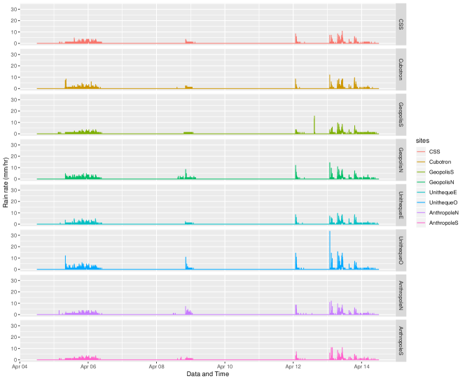
Figure 1: The eight time series of rain rate (unit: mm/hr) collected by Dryptich Pluvimate acoustic rain gauges every 30 seconds from April 4th to April 14th, 2016.

To handle the high-frequency data, the common practice is to make use of censored models to drive both the occurrence and the intensity processes. The models are also called truncated models by Allard, (2012), and the Tobit models (McDonald and Moffitt,, 1980) from econometrics. In the censored models, both the occurrence and intensity are driven by uncensored processes, where the dry events are zero values left-censored at a certain threshold, and the wet events are modeled by the process with a positive support.

Meta-Gaussian processes are the most popular way for the spatio-temporal dependence and non-Gaussian features of rainfall data (Ailliot et al.,, 2009; Kleiber et al.,, 2012; Baxevani and Lennartsson,, 2015). Although the methodologies provide high flexibility with regard to the spatio-temporal dependence, several limitations remain. First, the transformation of Gaussian processes is ad-hoc, ranging from simple power or logarithm transformations (Bell,, 1987; Glasbey and Nevison,, 1997; Durbán and Glasbey,, 2001) to complex Tukey g-and-h or hybrid Gamma transformations (Baxevani and Lennartsson,, 2015; Xu and Genton,, 2017). The efforts to achieve normality can be tedious. Second, the latent Gaussian processes make the interpretation difficult, especially when different transformations are suggested (Ailliot et al.,, 2015). Third, Gaussian processes are more suitable for denser spatial data rather than spatially sparse data, such as the multi-site high frequency time series.

Another popular way to quantify the spatio-temporal dependence in SPG is the vector autoregressive (VAR) processes (Hamilton,, 1994; Sigrist et al.,, 2012; Rasmussen,, 2013; Koch and Naveau,, 2015). The VAR framework has been widely used in a set of high-frequency data such as stock returns and brain signals. For precipitation, the state-of-arts censored VAR model is proposed by Koch and Naveau, (2015), for which the interpretation is easy and its likelihood-based inference is straightforward. However, this model only considers heteroscedastic Gaussian and meta-Gaussian error, which may not be adequate for data with skewed or heavy tailed distributions.

Therefore, we propose to use the skew-symmetric families (Azzalini,, 1985) in the censored VAR model. The skew-symmetric distributions have been generalized and applied in many fields of study (Azzalini and Capitanio,, 1999; Genton,, 2004; Azzalini,, 2013) in modeling the obviously non-Gaussian features, but rarely used in the SWG. The only application to SWG was investigated by Flecher et al., (2010), where the multivariate skew-normal distribution was adopted to model multiple atmospheric variables.

As an example, the density function of a univariate skew-t random variable is specified as

$$f_{\mathcal{ST}}(x;\xi,\omega,\alpha,\nu)=2t(u;\nu)T(\alpha u\sqrt{(\nu+1)(\nu+u^{2})};\nu+1),u=\frac{x-\xi}{\omega},$$ (1)

where $\xi$ and $\omega$ are the location and scale parameters, $\alpha$ is the skewness parameter, $\nu$, is the degree of freedom, $t(\cdot)$ is the standard t density function, and $T(\cdot)$ is the standard t distribution function.

The skew-normal distribution is a special case of the skew-t distribution when $\nu=\infty$. Similar to the normal or student-t distributions, $x$ can take any real value. In contrast, two extra parameters in the skew-t distribution controls the skewness and tail behavior. Another attractive feature of the skew-t distribution is the stochastic representation (Azzalini and Regoli,, 2012). A skew-t random variable $X$ can be expressed by hidden selective mechanism such that $X=(X_{1}|X_{2}>0)$, where $X_{1}$, $X_{2}$ are correlated t random variables with the same degree of freedom.

Since the generation mechanism behind the precipitation can be viewed as a hidden selection process, using a skew-symmetric distribution in modeling precipitation data produces nice physical interpretations, as will be further explained in Section 2.3. By incorporating skew-symmetric distributions and a censored VAR framework, we propose a new stochastic precipitation generator that

1) uses a single spatio-temporal model to simultaneously drive the precipitation occurrence and its intensity;

2) has direct interpretation to the precipitation process;

3) allows for flexible and tractable tail behaviors, which is crucial in modeling high-frequency precipitation data;

4) implies parsimonious parametrization and efficient data generation.

For the application to high-frequency precipitation data, recent studies also propose to use deep learning methods such as long short-term memory (LSTM) or other recurrent neural networks (RNN) (Shi et al.,, 2015, 2017). Although SPG focuses on reproducing the precipitation in the functional perspective, it is also important to show the results of prediction, especially comparing to these deep learning methods. We choose the multivariate LSTM networks as our competing methods to show the difference between our stochastic generators and the deep learning forecasters.

The rest of our paper is organized as follows. In Section 2, we introduce the new class of SPGs, provide model properties, and describe the inference procedure. In Section 3, we present simulation studies to validate our inference method and compare its performance to other models. In Section 4, we show the performance of the proposed SPGs on the high-frequency rainfall dataset collected at the University of Lausanne campus. In Section 5, we summarize our main results and discuss the potential limitations.

2 Censored skew-symmetric VAR models

2.1 Censored VAR models

Let $Y_{t}(s)$ be the precipitation amount observed at a site $s$ and time $t$, $s=1,\dots,N,t=1,\dots,T$. Collect $Y_{t}(s)$ as an $N\times 1$ vector $\textbf{Y}_{t}$. Then we specify the multi-site precipitation generator based on censored VAR as

$${Y}_{t}(s)=\begin{cases}\begin{array}[]{c}\boldsymbol{\beta}_{s}^{\prime}\textbf{Y}_{t-1}+{\varepsilon_{t}}(s),\\ 0,\end{array}&\begin{array}[]{c}\boldsymbol{\beta}_{s}^{\prime}\textbf{Y}_{t-1}+{\varepsilon_{t}}(s)>{u}_{t}(s),\\ \boldsymbol{\beta}_{s}^{\prime}\textbf{Y}_{t-1}+{\varepsilon_{t}}(s)\leq{u}_{t}(s),\end{array}\end{cases}$$ (2)

where $\boldsymbol{\beta}_{s}$ is an $N\times 1$ vector of autoregression coefficients for site $s$, ${u}_{t}(s)$ is the space-time varying cutoff vector representing the censoring threshold associated with the rain probability, and ${\varepsilon_{t}}(s)$ is the random error.

The censored VAR generator in (2) is originally proposed by Koch and Naveau, (2015). The model (2) differs from other SPGs since it avoids applying any ad-hoc transformation to the rainfall intensity when ${Y}_{t}(s)>0$. Therefore, the likelihood of ${Y}_{t}(s)$ has an explicit form and parameters in the model have direct interpretation to ${Y}_{t}(s)$.

The model (2) also differs from classical VAR model (Sims,, 1980; Hamilton,, 1994), where ${Y}_{t}(s)$ is not censored and the error term $\varepsilon_{t}(s)$ is assumed to be white noise with zero mean and constant variance. Here, a more general case is considered for $\varepsilon_{t}(s)$ by letting $\varepsilon_{t}(s)=\sigma_{t}z_{t}(s)$. In this setting, $z_{t}(s)$ are independent, but the error terms $\varepsilon_{t}(s)$ are not independent in general.

2.2 Censored VAR models with skew-symmetric errors

The independent random variables $z_{t}(s)$ in Koch and Naveau, (2015) is assumed to follow a standard normal distribution and the standard deviations are modeled with other atmospheric explanatory variables by a linear regression. However, these explanatory variables are often either unavailable or hard to choose in practice. This issue becomes more problematic when they assume that $z_{t}(s)$ is normally distributed because the right-skewed and heavy-tailed features of the rainfall data can be only explained by $\sigma_{t}$. Then the entire dynamics of the SPG will be heavily influenced by the selected explanatory variables.

Therefore, we consider another random error that is flexible with the skewness and tail behavior so that the explanatory variables are not required. Instead of a normal distribution, we assume that $z_{t}(s)$ follows a family of skew-symmetric distributions (Azzalini,, 2013) with zero mean and unit variance. As we mentioned in (1), $z_{t}(s)$ itself already describes the skewed and heavy-tailed features, rather than relying on the other explanatory variables.

For the standard deviations, we allow for heteroscedasticity with a temporally varying standard deviation $\sigma_{t}$. The idea of heteroscedasticity is widely used to predict high-frequency data such as wind power and stock-returns (Engle,, 1982; Bollerslev,, 1986; Taylor et al.,, 2009), such as the (generalized) autoregressive conditionally heteroscedastic (ARCH/GARCH) models. Specifically, we assume that $\sigma_{t}=b_{0}+b_{1}\bar{Y}_{t-1}$, where $\bar{Y}_{t-1}=\sum\limits_{s=1}^{N}{Y}_{t-1}(s)/N$ and $b_{0},b_{1}\geq 0$ to avoid a negative variance.

To describe the distribution of $z_{t}(s)$, three candidates in the skew-symmetric family are commonly used: the skew-normal distribution (Azzalini,, 1985), the skew-t distribution (Branco and Dey,, 2001; Azzalini and Capitanio,, 2003), and the skew-Cauchy distribution (Behboodian et al.,, 2006). Since the skew-t distribution with the degree of freedom $\nu$ includes the skew-normal and the skew-Cauchy distribution as special cases, hereafter we mainly discuss the properties of the skew-t distribution. The results from the skew-normal and skew-Cauchy distributions can be simply obtained by replacing $\nu$ with $\infty$ and $1$, respectively.

We assume that $z_{t}(s)\overset{\mathrm{iid}}{\sim}\mathcal{ST}(\xi,\omega,\alpha,\nu)$ with density function (1). For the skew-t distribution, $\xi$ is not the mean and $\omega$ is not the standard deviation. Instead, $\mathbb{E}\{z_{t}(s)\}=\xi+\omega b_{\nu}\delta$ and $\mathrm{var}\{z_{t}(s)\}=\omega^{2}\left\{\frac{\nu}{\nu-2}-(b_{\nu}\delta)^{2}\right\}$, where $b_{\nu}=\frac{\sqrt{\nu}\Gamma(\frac{1}{2}(\nu-1))}{\sqrt{\pi}\Gamma(\frac{1}{2}\nu)}$ and $\delta=\frac{\alpha}{\sqrt{1+\alpha^{2}}}$. To obtain zero mean and unit variance, we set $\omega=\frac{1}{\sqrt{\frac{\nu}{\nu-2}-(b_{\nu}\delta)^{2}}}$ and $\xi=-\frac{b_{\nu}\delta}{\sqrt{\frac{\nu}{\nu-2}-(b_{\nu}\delta)^{2}}}$. Therefore, the scaled skew-t distribution only depends on the skewness parameter $\alpha$ and the degree of freedom $\nu$. The corresponding density function and distribution are denoted by $f_{\mathcal{SST}}(\cdot)=f_{\mathcal{SST}}(x;\alpha,\nu)$ and $F_{\mathcal{SST}}(\cdot)=F_{\mathcal{SST}}(x;\alpha,\nu)$, respectively.

2.3 Model implications and interpretations

The proposed model is flexible and all the parameters in model (2) have natural interpretations. For example, a higher $\nu\in\mathbb{R}^{+}$ and $\alpha\in\mathbb{R}$ imply a lighter tail and larger right-skewness, respectively; $\sigma_{t}$ introduces the heteroscedasticity; the autoregression matrix $B=(\boldsymbol{\beta}_{s})_{s=1}^{N}=(\beta_{ij})_{N\times N}$ controls the spatio-temporal dependence, and $u_{t}(s)$ is the threshold that determines the wet or dry probability.

We can derive several important precipitation probabilities conditional on previous observations. First, the conditional dry probability at site $s$ and time $t$ is

$${\footnotesize\mathbb{P}\{Y_{t}(s)=0|\textbf{Y}_{t-1}=\textbf{y}_{t-1}\}=\mathbb{P}\{\varepsilon_{t}(s)\leq u_{t}(s)-\boldsymbol{\beta}^{\prime}_{s}\textbf{y}_{t-1}\}=F_{\mathcal{SST}}\left(\frac{u_{t}(s)-\boldsymbol{\beta}^{\prime}_{s}\textbf{y}_{t-1}}{b_{0}+b_{1}\bar{Y}_{t-1}}\right).}$$

Hence, a higher dry probability can be reached by either decreasing $b_{0},b_{1}$ or $\alpha$, or by increasing $u_{t}(s)$ or $\nu$. In particular, if $\textbf{Y}_{t-1}=\textbf{0}$, then we have the consecutive dry probability $\mathbb{P}(Y_{t}(s)=0|\textbf{Y}_{t-1}=\textbf{0})=F_{\mathcal{SST}}\left(\frac{u_{t}(s)}{b_{0}}\right)$.

Since the random variables $z_{t}(s)$ are independent, the simultaneously dry probability at multiple sites is the product of marginal probabilities. Therefore, once we plug in the estimated parameters for those probabilities, which are conditional on previous events, we can immediately obtain the dry/wet probability (rainfall occurrence), consecutive dry/wet probability (distribution of the dry/wet spell length), and the simultaneous dry/wet probability for multiple sites (rainfall spatial pattern).

The SPG in model (2) possesses both flexible statistical properties and nice physical interpretations. We illustrate these by representing model (2) as a state-space model, i.e., a two-layer model where the transition from zero to positive values is driven by the selection mechanism of the skew-t distribution. The equivalent model can be specified as:

$${Y}_{t}(s)=\begin{cases}\begin{array}[]{c}{X}_{t}(s),\\ 0,\end{array}&\begin{array}[]{c}{X}_{t}(s)>{u}_{t}(s),\\ {X}_{t}(s)\leq{u}_{t}(s),\end{array}\end{cases}$$ (3)

$${X}_{t}(s)=g(\textbf{X}_{t-1})+\begin{cases}\begin{array}[]{c}{Z}_{t}(s),\\ -{Z}_{t}(s),\end{array}&\begin{array}[]{c}{W}_{t}(s)>0,\\ {W}_{t}(s)\leq 0,\end{array}\end{cases}$$ (4)

where the threshold ${u}_{t}(s)$ is deterministic, the latent autoregressive process ${X}_{t}(s)$ depends on a function of $\textbf{X}_{t-1}$ called $g(\textbf{X}_{t-1})$, and the random errors are controlled by two processes, ${Z}_{t}(s)$ and ${W}_{t}(s)$. The proof for the equivalence between Equation (2) and Equations (3) and (4) is given in the Supplements.

In meteorology, it is well known that the precipitation comes from condensed atmospheric water vapor, which is formed at certain temperatures and moisture conditions, and then falls as observable rainfall due to gravity. Our equations (3) and (4) describe this physical process.

Equation (3) is the measurement equation, which we call the ground layer model. It describes the amount of condensed atmospheric water vapor $X_{t}(s)$ that becomes precipitation $Y_{t}(s)$ at time $t$ and location $s$. The wet-dry threshold ${u}_{t}(s)$ represents the necessary conditions for rainfall, defined as the minimum condensed water vapor required for observable rainfall, i.e., to reach the detection limit of the measuring instrument. Equation (4) is the transition equation, which we call the atmospheric layer model. It describes the formation of condensed water vapor in the atmosphere. The current condensed water vapor $X_{t}(s)$ is modeled using past observations at all locations $g(\textbf{X}_{t-1})$, with random fluctuations ${Z}_{t}(s)$ that represent the new formation and dissolution of condensed water vapor. The fluctuation ${Z}_{t}(s)$ is not just the symmetric random noise, but is driven by a hidden selection process ${W}_{t}(s)$, which represents certain meteorological conditions, known as weather fronts such as temperature and moisture. Although the distributions of their elements, $Z_{t}(s)$ and $W_{t}(s)$, are both symmetric, when they are correlated, the distribution of $X_{t}(s)$ becomes skewed. This representation explains that our model is suitable for data that are censored and skewed. Therefore, the proposed SPG can potentially simulate realistic precipitation observations.

2.4 Inference and computational issues

The inference of model (2) is straightforward as it belongs to the generalized Tobit model (McDonald and Moffitt,, 1980). We show in the supplements that the log-likelihood, $\ell(\boldsymbol{\theta}|\textbf{y}_{1},\dots,\textbf{y}_{T})$, can be written as

$${\footnotesize\begin{array}[]{r@{}l}\ell(\boldsymbol{\theta}|&\textbf{y}_{1},\dots,\textbf{y}_{T})=\\ &\sum_{t=2}^{T}\sum_{s=1}^{N}\mathbbm{1}_{\{y_{t}(s)>0\}}\left[\log\left\{f_{\mathcal{SST}}\left(\frac{y_{t}(s)-\boldsymbol{\beta}_{s}^{\prime}\textbf{y}_{t-1}}{b_{0}+b_{1}\bar{Y}_{t-1}}\right)\right\}-\log\left\{b_{0}+b_{1}\bar{Y}_{t-1}\right\}\right]\\ &+\sum_{t=2}^{T}\sum_{s=1}^{N}\mathbbm{1}_{\{y_{t}(s)=0\}}\log\left\{F_{\mathcal{SST}}\left(\frac{{u}_{t}(s)-\boldsymbol{\beta}_{s}^{\prime}\textbf{y}_{t-1}}{b_{0}+b_{1}\bar{Y}_{t-1}}\right)\right\},\end{array}}$$ (5)

where $\boldsymbol{\theta}$ is the vector of parameters to be estimated, $\mathbbm{1}_{\{y_{t}(s)>0\}}$ is an indicator function that takes a value of $1$ when $y_{t}(s)>0$ and $0$ otherwise, $f_{\mathcal{SST}}(\cdot;\alpha,\nu)$ is the scaled skew-t density function, and $F_{\mathcal{SST}}(\cdot;\alpha,\nu)$ is the distribution function.

To achieve a robust estimation of the unknown parameters with some meaningful interpretations, some of the values in (5) are further parameterized. First, we estimate the cutoffs, i.e., the censoring thresholds, by taking the seasonality into account. Similar to Sun and Stein, (2015), the estimated cutoff $\hat{u}_{t}(s)$ is chosen to be the quantile $q_{t}(s)$, corresponding to the probabilities $1-{O}_{t}(s)$, where $O_{t}(s)$ is the precipitation occurrence that takes a zero or one value and is fitted by logistic regression at each site $s$ with the binary time series data. The estimated occurrence is denoted by $\hat{O}_{t}(s)$. Then, the cutoff is estimated as $\hat{q}_{t}(s)$, the marginal sample quantile of $Y_{t}(s)$ corresponding to the probability $1-\hat{O}_{t}(s)$. Since $Y_{t}(s)$ is always larger than the real precision limit $u_{r}$, the cutoffs are not supposed to be smaller than $u_{r}$. Therefore, we have $\hat{u}_{t}(s)=\max\{\hat{q}_{t}(s),u_{r}\}$. The covariates include harmonic terms for day-of-year seasonality. Here, we assume that

$${\begin{array}[]{r@{}l}\mathrm{logit}[&\mathbb{P}\{O_{t}(s)=1\}]=\sum_{j=1}^{H}\left\{\gamma_{1j}(s)+\gamma_{2j}(s)\sin\left(2\pi j\frac{d(t)}{365}\right)+\gamma_{3j}(s)\cos\left(2\pi j\frac{d(t)}{365}\right)\right\},\end{array}}$$ (6)

where $d(t)\in\{1,\dots,365\}$ denotes the day within each year, and the value of $H$ is chosen by Akaike information criterion (AIC (Akaike,, 1998)).

To quantify the spatial dependence and make the estimation of the autoregressive parameters computationally feasible, we further parameterize the $N\times N$ matrix $B$ using the idea in Sigrist et al., (2012). Since we do not observe nonstationarity and anisotropy, we consider a simple parametrization of Sigrist et al., (2012) that models $\beta_{ij}$ by a spatial covariance functions of Whittle-Matérn type i.e., $\beta_{ij}(\phi,\rho)=(\phi d_{ij}/\rho)K_{1}(d_{ij}/\rho)$, where $K(\cdot)$ is the modified Bessel function of the second kind, $\phi,\rho>0$ are scaling parameters, and $d_{ij}$ is the distance between locations $i$ and $j$. Thus we account for the spatial dependence and assume that faraway sites are less correlated. Furthermore, to make sure the process is temporally stationary, the largest eigenvalue of matrix $B$ should be less than 1. Here, we use a sufficient condition for $B$ by constraining $\phi/\rho<\frac{1}{N\max_{ij}(d_{ij})}$. Note that the condition only holds if $B$ is a valid covariance matrix.

The final unknown parameters in the (5) are $\boldsymbol{\theta}=(\phi,\rho,b_{0},b_{1},\alpha,\nu)^{T}$. Although we reduce the number of unknown parameters to six, the optimization of the likelihood that can only be achieved numerically is still potentially unstable. Thus, we consider several different numerical optimization methods: two derivative-free algorithms (COBYLA and Nelder-Mead) and two derivative-based algorithms (BFGS and CG). Many literatures point out that the optim function in R is not numerically stable, especially when a re-parameterization exists (Mullen,, 2014; Nash and Varadhan,, 2011; Nash, 2014a, ). Therefore, we employ two recently developed R packages, nloptr (Johnson,, 2014) and Rcgmin (Nash, 2014b, ), as a substitution of optim. To make sure that the optimization reaches the global maximum, we use different optimization algorithms with multiple sets of initial values until we get the same optimized values. The sn packages (Azzalini,, 2011) were used to evaluate $f_{\mathcal{SST}}(\cdot)$ and $F_{\mathcal{SST}}(\cdot)$. We also notice that the estimation of the degree of freedom $\nu$ is typically not numerically stable as in other similar problems, one can evaluate the likelihood over a sequence of values of $\nu$. The best $\nu$ can be selected according to the maximized likelihood function.

3 Simulation studies

We designed a simulation study to validate the inference procedure introduced in Section 2.4 and compare to the original censored VAR models proposed by Koch and Naveau, (2015) using the Gaussian dynamics. We generate multiple synthetic datasets from the censored VAR model (2) at the eight locations shown in Figure 1, where $z_{t}(s)$ follows a skew-t distribution. By choosing different skewness parameter $\alpha$ and the degree of freedom $\nu$, the generated data can approximate the Koch and Naveau, (2015) as a special case by letting $\alpha=0$ and $\nu$ be a large value. In the simulation, we set $\nu=20$ to be large and two other different degrees of freedom $\nu=3,7$ for comparison. In addition, we set skewness parameter, $\alpha=5$ to represent the skewed data and set $(T,N,\phi,\rho,b_{1},b_{2})=(10000,3,1/3,1,0.5,0.5)$. The sample sizes, $T$ and $N$, are the same as the application in Koch and Naveau, (2015) for comparison reason and other parameters are similar to the estimated values from the Lausanne precipitation data in order to mimic a real application.

We fit the models with skew-t and Gaussian dynamics to the synthetic datasets. The summary of estimated values based on 50 independent realizations are shown in Table S1 of the Supplements. With different dynamics, the optimized common factors, such as $b_{0}$ and $b_{1}$, are different as well. The results show that Gaussian dynamics tends to overestimate the $b_{0}$ and $b_{1}$ so that the overestimated variance will compensate the light tail of Gaussian distribution.

Then, we generate 50 parametric bootstrap samples from the median of the fitted values and calculate the mean of the root-mean-squared errors (MRMSE) for the six scenarios. Specifically, the MRMSE is defined as $\frac{1}{50}\sum_{k=1}^{50}\sqrt{\frac{1}{NT}\sum_{t=1}^{T}\sum_{s=1}^{N}\left\{Y_{t}(s)-Y^{B}_{kt}(s)\right\}^{2}}$, where $Y_{t}(s)$ and $Y^{B}_{kt}(s)$ denote the synthetic data and the $k$-th bootstrap sample at time $t$ and location $s$, respectively. The results are shown in Table 1.

Table 1: Summary of the simulation study results. The MRMSEs are presented as percentages (%). The first row lists the parameter setups for $(\nu,\alpha)$. The second and third rows list MRMSE of the censored VAR generators with the skew-t and Gaussian dynamics, respectively. The last row shows the MRMSE ratio of the Gaussian to skew-t models.

Scenarios $(\nu,\alpha)$	$(3,0)$	$(3,5)$	$(7,0)$	$(7,5)$	$(20,0)$	$(20,5)$
Skew-t	$32.91$	$54.85$	$26.01$	$49.27$	$24.23$	$38.55$
Gaussian	$35.41$	$59.32$	$27.03$	$52.30$	$24.58$	$39.70$
Ratio	$1.076$	$1.082$	$1.039$	$1.061$	$1.014$	$1.030$

From Table 1, we see that when $\nu$ is large and $\alpha=0$, two models produce similar results. Even in this case, the MRMSE values of our model are slightly smaller than those of the model with the Gaussian dynamics since $\nu$ is still smaller than infinity. In contrast, when $\alpha$ is positive and $\nu$ is small, the difference in MRMSEs is more significant, and the Gaussian model becomes less reliable.

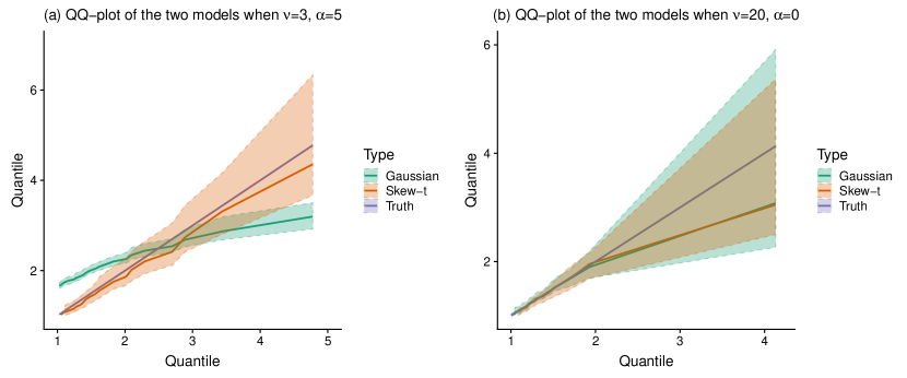
Figure 2: Quantile-quantile (QQ) plot between the synthetic (purple curve) and 50 parametric bootstrap samples using (a) a skew-t error (orange region) and (b) a Gaussian error (green region). The solid lines are the median curves and the shaded areas are the 95% confidence intervals.

To visualize the difference statistically, we draw quantile-quantile (QQ) plots between the synthetic data and the parametric bootstrap samples for two scenarios, $(\nu,\alpha)=(20,0)$ and $(\nu,\alpha)=(3,5)$. The results are shown in Figure 2. Not surprisingly, the Gaussian model cannot reproduce the heavy-tailed and right-skewed behavior that results from a large skewness parameter and a small degree of freedom. In both cases, our model with the skew-t errors successfully reproduces these statistical properties.

Incorrectly assuming a Gaussian model for the data also affects the estimation of other important statistical properties of rainfall. As we mentioned, Gaussian model typically overestimates $b_{0}$ and $b_{1}$ of heavy-tailed data in order to produce a high rainfall intensity. However, as we explained in Section 2.3, a large $b_{0}$ and $b_{1}$ also leads to a low dry probability. Therefore, failing to correctly specify the degree of freedom will underestimate the dry probability as well, as shown in Figure S2 of the Supplements, where the distribution of the dry probability is obtained from the bootstrap samples. Therefore, only relying on the heteroscedastic standard deviations, without considering a right-skewed and heavy-tailed error term, is not enough to capture the statistical properties of high-frequency rainfall patterns and the stochastic simulations will not be realistic.

4 Application to Lausanne precipitation data

The motivating data, as shown in Figure 1, were collected by GAIA Lab, Institute of Earth Surface Dynamics (IDYST), the University of Lausanne in 2016 using eight Pluvimate acoustic rain gauges (Collister and Mattey,, 2008). The detailed description of the Pluvimate rain gauges can be found in Benoit et al., (2018). This new instrument can measure precipitations at a $0.01$mm and 30 second resolution with the standard rain rate unit, mm/hr. From April 4th to April 14th, 2016, a total number of 230,400 observations were recorded by the network of eight rain gauges located within a radius of 1 km, as shown in Figure S2 in the Supplements.

Table 2 and Figure S3 in the Supplements show the distribution of the collected rainfall data. Most of the observations (92.4%) were zeros, corresponding to no rain or dry events. Most of the rain intensities are below 5 mm/hr, while at some periods there are heavy rainfall with the rain rate around $10$ mm/hr. We also observe that the highest rain rate reached more than $30$ mm/hr. The QQ-plot also shows that these rainfall data are zero-inflated, right-skewed, and heavy-tailed and completely deviate from Gaussian distribution.

Table 2: Distribution of the collected rainfall data.

Rain rate (mm/hr)	$=0$	$(0,1.2]$	$(1.2,5]$	$(5,10]$	$(10,33.6]$
Percentage	$92.40\%$	$5.55\%$	$1.84\%$	$.19\%$	$.02\%$

We fitted the time-varying cutoffs as described in Section 2.4 with the lowest positive rate rate $u_{r}=1.2$ using the glm package in R and fitted the other parameters by the methods mentioned in the Section 2.4. The fitted results are shown in Table 3, along with the results of the Gaussian model for comparison purposes. We can see that the maximum likelihood estimators (MLEs) of both the degree of freedom $\nu$ and the skewness parameter $\alpha$ are small. Similar to the simulation study, the values of $b_{0}$ and $b_{1}$ estimated from the Gaussian model are larger than those estimated from the skew-t model.

Table 3: Maximum likelihood estimators (MLEs) from the censored VAR model with skew-t and Gaussian errors.

Parameters	Skew-t Errors		Gaussian Errors
	Est	95%CI	Est	95%CI
$\phi$	$.146$	$(.143,.149)$	$.163$	$(.158,.168)$
$\rho$	$1.395$	$(1.211,1.610)$	$0.879$	$(0.786,0.984)$
$b_{0}$	$.457$	$(.451,.463)$	$.474$	$(.470,.478)$
$b_{1}$	$.257$	$(.250,.271)$	$.281$	$(.273,.290)$
$\alpha$	$.034$	$(.022,.053)$
$\nu$	4

4.1 Conditional rainfall generation

From the fitted model, we can generate 50 parametric bootstrap samples of the high-frequency rainfall. Each sample can be viewed as a synthetic realization of the 30-second rainfall data. To examine the similarity of the simulated samples to the real data, we use a one-step-ahead conditional simulation, which generates data conditional on observations one step in the past. The main goal here is to reproduce the statistical properties of the real data, we use a QQ plot shown in Figure 3, to compare the real data with the bootstrap samples from the two models. From the results, both models can reproduce the low-intensity rainfall well statistically. However, in terms of the heavy rainfall (defined as having an intensity larger than 10 mm/hr), the 95% confidence band of the Gaussian model significantly underestimates the precipitation, whereas the skew-t model captures the heavy tail very well.

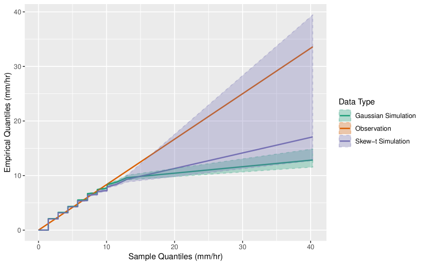
Figure 3: Quantile-quantile (QQ) plot between the observed rainfall (purple curve) and 50 parametric bootstrap samples using a skew-t error (orange region) and a Gaussian error (green region). The solid lines are the median curves and the shaded areas are the 95% confidence intervals.

The spatio-temporal patterns of rainfall occurrence are assessed by the rain concurrences and dry probability. Figure 4 shows the histogram of simultaneously rainy locations for both the observed and simulated rainfall data, from which we can see the spatial dependences among multisite rainfall occurrences. The simulated histograms combines all of the 50 parametric bootstrap samples. The eight locations are usually all dry. In this case, the simulated data slightly overestimate the counts. In contrast, when at least one location is rainy, the simulated data have fewer counts than real observations, which means the spatial correlation is slightly underestimated. Overall, the rain concurrences are reproduced reasonably well by our model.

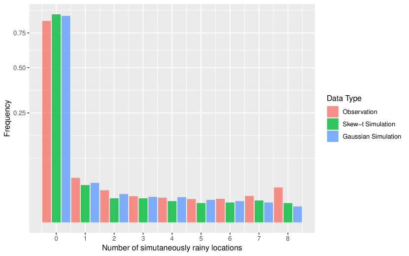
Figure 4: Histogram showing the simultaneously rainy locations. Each bar represents how many corresponding events happen in time. The y-axis is shown in the square root scale.

The temporal dependence of rainfall occurrence can be reflected by the dry/wet spell length and conditional dry/wet probability. The dry/wet spell length is less important for the high-frequency data of only ten days and thus we only show the conditional probabilities. Table 4 displays the four different conditional probabilities. Overall, the simulated data can reproduce the conditional dry/wet probability well. However, the simulated data tend to underestimate the probability of transition between wet and dry. This is an expected result of the hard thresholding effect. Nevertheless, it does not affect much on the overall distribution of the rainfall intensity. If it is crucial to accurately reproduce the dry or wet probability, a separate model for rainfall occurrences might be a better choice.

Table 4: Conditional probabilities from the observed rainfall data and the mean ($\pm 1.96\times$standard deviation) of the conditional probabilities from 50 parametric bootstrap samples generated using a skew-t and Gaussian model.

	Wet$|$Wet	Dry$|$Wet	Wet$|$Dry	Dry$|$Dry
Skew-t Dynamics	.976($\pm.0045$)	.024($\pm.0045$)	.024($\pm.0045$)	.976($\pm.0045$)
Gaussian Dynamics	.974($\pm.0062$)	.026($\pm.0062$)	.026($\pm.0062$)	.974($\pm.0062$)
Observation	.971	.029	.029	.971

Compared to the Gaussian model, the major advantage of the skew-t model is that it can reproduce both dry events and heavy rainfall. However, since the Gaussian and skew-t models we considered use the same spatio-temporal modeling strategy, i.e., the VAR model with a time-varying threshold, the spatio-temporal properties of the rainfall occurrences do not show much difference.

4.2 Short-term rainfall prediction

A SWG is not meant for prediction but generate multiple realizations with similar statistical properties of the real data. However, we can provide some predictive information by the mean of quantiles of multiple realizations. We give an example here to illustrate the performance of our model in prediction, compared to a multivariate LSTM model as a popular deep learning-based model for time series prediction. We use the last day of rainfall ($5,760$ points) at each location as the testing set and other data as the training set. We re-fit our model using the training data and fit the LTSM model using one hidden layer of $100$ LSTM units with rectified linear unit (ReLU) activation, Adam optimization algorithm, and mean squared error (MSE) as the loss function. The LSTM model is run on Keras functional API with 100 epoch in Python.

As a precipitation generator, our model can simultaneously generate 50 realizations and we use the mean of 50 realizations as our predictor in the comparison. We also compute the $95\%$ prediction band by the quantiles of the 50 realizations to show the uncertainties. In terms of the MSE, the result of our model (MSE$=0.099$) outperforms the LSTM (MSE$=0.126$). However, if we pick a single realization of our model, the MSE of LSTM is better than any of the realizations (MSE$=0.204$ based on the best MSE of single realization). To visualize the results, in Figure 5, we show one heavy rain event in the evening of April 13 and $95\%$ prediction band from our model as there is almost no rain at other time. The results show that the 95% prediction band covers the observed rainfalls. Also, the prediction of LSTM is more variable with a few obvious peaks far from the observed values. Instead, our predictor is more stable since it collects the mean of 50 realizations.

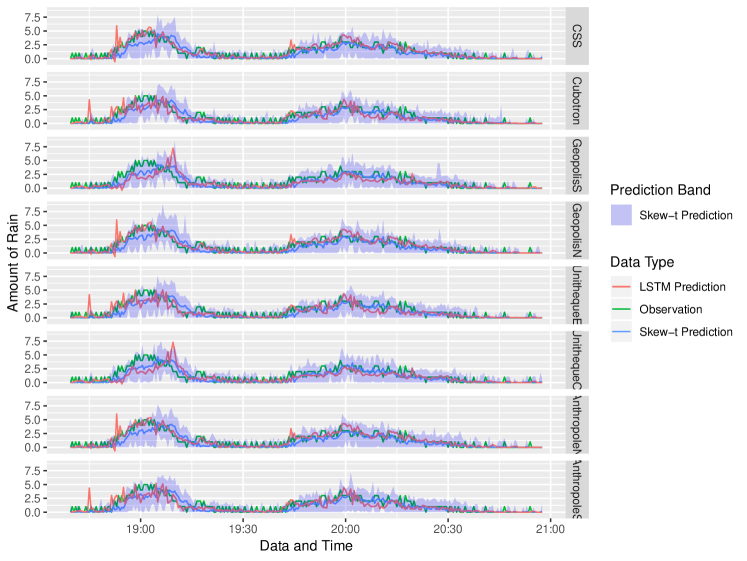
Figure 5: The performance of predicted rain rate (mm/hr) (with uncertainties) during a heavy rainfall period on April 13, 2016. The blue line and blue band are the mean prediction and $95\%$ prediction band from our model, respectively. The red line is the prediction from LSTM model. The green line is the last day of rainfall observation as the truth.

From the results, two main differences between LSTM predictor and our stochastic precipitation generator are noticed, even though both of the models provide good prediction. Firstly, a SWG can serve as a predictor by generating multiple independent predictors, which can be used to quantify the uncertainties. But with regards to a single predictor, LSTM can perform better. Secondly, as many other deep learning methods, the prediction of LSTM is done via optimizing certain loss function, e.g. MSE, thus the results are hard to interpret than our model-based prediction. For example, the predicted values from LSTM model can be negative values. Although we can treat the negative value as zero by the ReLU activation function in the output layer, we lose some meaningful interpretations of the rainfall properties.

5 Discussion

In this study, we proposed a new SWG for high frequency rainfall that is capable of reproducing large quantities of zeros and extreme values. This model utilizes skew-t random variables with a censoring mechanism to simultaneously drive both the occurrence and intensity of rainfall. By applying a VAR model for spatio-temporal dependence, the inference can be achieved simply by maximizing the likelihood function.

We applied the SWG to a rarely assessed and fine-scale precipitation dataset collected by an acoustic rain gauges every 30 seconds and spatially around $10-100$ meters. The results show that the SPG can generate high-intensity rainfall better than the baseline model with Gaussian errors. We also show that our SWG can be used for prediction purposes and its performance is comparable to LSTM, a modern deep learning method. Compared to the LSTM, our SWG can provide uncertainties and is more interpretable.

Although we only consider the VAR framework with a linear spatio-temporal dependence, the model can be generalized by considering other spatio-temporal dependences. One situation was discussed in Tadayon and Khaledi, (2015), where a Bayesian hierarchical model was used with only skew-normal error and purely spatial dependence. Another possibility is to use a censored multivariate skew-symmetric distribution. However, the associated inference might be challenging, since likelihood functions do not have a closed form as in our model. The main reason is that skew-symmetric random variables do not retain all of the desired properties when they become Gaussian or student-t random variables, e.g., they are not closed under convolution or conditioning. Thus, some existing results under certain assumptions, such as additive models, or solutions derived from conditional distributions, such as the Kriging predictor, would no longer hold in skew-symmetric cases.

We parameterize the autoregression matrix, which reduces the number of parameters while taking spatial information into account. Although such a parameterization fits our purpose well, some limitations exist. First, we selected a covariance function to construct the autoregression matrix, which implies that the single-site temporal correlation is homogenous across many locations. Second, the correlation matrix only allows for a positive correlation among locations, whereas an autoregression matrix could also have negative correlations. Last, we use a sufficient condition for the parameters in the spatial covariance function to satisfy the temporally stationary condition. However, it is more favorable to have a necessary and sufficient condition to ensure the stationarity. Thus if only less sites are assessed it is better to estimate the autoregression matrix in element-wise.

6 Acknowledgement

This research was supported by King Abdullah University of Science and Technology (KAUST), Office of Sponsored Research (OSR) under Award No: OSR-2019-CRG7-3800. The dataset used in this study is provided by GAIA Lab, Institute of Earth Surface Dynamics (IDYST), the University of Lausanne. We acknowledge their efforts for collecting the data.

SUPPLEMENTARY MATERIAL

Source code:

The source code in this work is available on the following repository:
https://github.com/aleksada/MultisiteHighFreqPG. (website)

Proofs, figures, and tables:

The supplementary material consists of the proofs of Equations (4) and (5) and additional figures and tables. (.pdf file)

References

- Ailliot et al., (2015) Ailliot, P., Allard, D., Monbet, V., and Naveau, P. (2015). Stochastic weather generators: an overview of weather type models. Journal de la Société Française de Statistique, 156(1):101–113.
- Ailliot et al., (2009) Ailliot, P., Thompson, C., and Thomson, P. (2009). Space-time modelling of precipitation by using a hidden Markov model and censored Gaussian distributions. Journal of the Royal Statistical Society: Series C (Applied Statistics), 58(3):405–426.
- Akaike, (1998) Akaike, H. (1998). Information theory and an extension of the maximum likelihood principle. In Selected Papers of Hirotugu Akaike, pages 199–213. Springer.
- Allard, (2012) Allard, D. (2012). Modeling spatial and spatio-temporal non Gaussian processes. In Advances and Challenges in Space-time Modelling of Natural Events, pages 141–164. Springer.
- Azzalini, (1985) Azzalini, A. (1985). A class of distributions which includes the normal ones. Scandinavian Journal of Statistics, pages 171–178.
- Azzalini, (2011) Azzalini, A. (2011). R package sn: The skew-normal and skew-t distributions (version 0.4-17). URL http://azzalini. stat. unipd. it/SN, 20.
- Azzalini, (2013) Azzalini, A. (2013). The Skew-Normal and Related Families, volume 3. Cambridge University Press.
- Azzalini and Capitanio, (1999) Azzalini, A. and Capitanio, A. (1999). Statistical applications of the multivariate skew normal distribution. Journal of the Royal Statistical Society: Series B (Statistical Methodology), 61(3):579–602.
- Azzalini and Capitanio, (2003) Azzalini, A. and Capitanio, A. (2003). Distributions generated by perturbation of symmetry with emphasis on a multivariate skew t-distribution. Journal of the Royal Statistical Society: Series B (Statistical Methodology), 65(2):367–389.
- Azzalini and Regoli, (2012) Azzalini, A. and Regoli, G. (2012). Some properties of skew-symmetric distributions. Annals of the Institute of Statistical Mathematics, 64(4):857–879.
- Baxevani and Lennartsson, (2015) Baxevani, A. and Lennartsson, J. (2015). A spatiotemporal precipitation generator based on a censored latent Gaussian field. Water Resources Research, 51(6):4338–4358.
- Behboodian et al., (2006) Behboodian, J., Jamalizadeh, A., and Balakrishnan, N. (2006). A new class of skew-Cauchy distributions. Statistics & Probability Letters, 76(14):1488–1493.
- Bell, (1987) Bell, T. L. (1987). A space-time stochastic model of rainfall for satellite remote-sensing studies. Journal of Geophysical Research: Atmospheres, 92(D8):9631–9643.
- Benoit et al., (2018) Benoit, L., Allard, D., and Mariethoz, G. (2018). Stochastic rainfall modeling at sub-kilometer scale. Water Resources Research, 54(6):4108–4130.
- Bollerslev, (1986) Bollerslev, T. (1986). Generalized autoregressive conditional heteroskedasticity. Journal of Econometrics, 31(3):307–327.
- Boschert and Rosen, (2016) Boschert, S. and Rosen, R. (2016). Digital twin–the simulation aspect. In Mechatronic Futures, pages 59–74. Springer.
- Branco and Dey, (2001) Branco, M. D. and Dey, D. K. (2001). A general class of multivariate skew-elliptical distributions. Journal of Multivariate Analysis, 79(1):99–113.
- Chan et al., (2016) Chan, S., Kendon, E., Roberts, N., Fowler, H., and Blenkinsop, S. (2016). The characteristics of summer sub-hourly rainfall over the southern uk in a high-resolution convective permitting model. Environmental Research Letters, 11(9):094024.
- Collister and Mattey, (2008) Collister, C. and Mattey, D. (2008). Controls on water drop volume at speleothem drip sites: An experimental study. Journal of Hydrology, 358(3-4):259–267.
- Durbán and Glasbey, (2001) Durbán, M. and Glasbey, C. (2001). Weather modelling using a multivariate latent Gaussian model. Agricultural and Forest Meteorology, 109(3):187–201.
- El Saddik, (2018) El Saddik, A. (2018). Digital twins: The convergence of multimedia technologies. IEEE MultiMedia, 25(2):87–92.
- Engle, (1982) Engle, R. F. (1982). Autoregressive conditional heteroscedasticity with estimates of the variance of united kingdom inflation. Econometrica: Journal of the Econometric Society, pages 987–1007.
- Falconer and Mitchell, (2012) Falconer, G. and Mitchell, S. (2012). Smart city framework. Cisco Internet Business Solutions Group (IBSG), pages 1–11.
- Flecher et al., (2010) Flecher, C., Naveau, P., Allard, D., and Brisson, N. (2010). A stochastic daily weather generator for skewed data. Water Resources Research, 46(7).
- Gabriel and Neumann, (1962) Gabriel, K. and Neumann, J. (1962). A Markov chain model for daily rainfall occurrence at Tel Aviv. Quarterly Journal of the Royal Meteorological Society, 88(375):90–95.
- Genton, (2004) Genton, M. G. (2004). Skew-Elliptical Distributions and Their Applications: A Journey Beyond Normality. CRC Press.
- Gilchrist, (2016) Gilchrist, A. (2016). Industry 4.0: The Industrial Internet of Things. Springer.
- Glasbey and Nevison, (1997) Glasbey, C. and Nevison, I. (1997). Rainfall modelling using a latent Gaussian variable. In Modelling Longitudinal and Spatially Correlated Data, pages 233–242. Springer.
- Hamilton, (1994) Hamilton, J. D. (1994). Time Series Analysis, volume 2. Princeton University Press.
- Heckman, (1976) Heckman, J. J. (1976). The common structure of statistical models of truncation, sample selection and limited dependent variables and a simple estimator for such models. In Annals of Economic and Social Measurement, Volume 5, number 4, pages 475–492. NBER.
- Johnson, (2014) Johnson, S. (2014). The nlopt nonlinear-optimization package [software].
- Katz, (1977) Katz, R. W. (1977). Precipitation as a chain-dependent process. Journal of Applied Meteorology, 16(7):671–676.
- Kleiber et al., (2012) Kleiber, W., Katz, R., and Rajagopalan, B. (2012). Daily spatiotemporal precipitation simulation using latent and transformed gaussian processes. Water Resources Research, 48:W01523.
- Koch and Naveau, (2015) Koch, E. and Naveau, P. (2015). A frailty-contagion model for multi-site hourly precipitation driven by atmospheric covariates. Advances in Water Resources, 78:145–154.
- Mary et al., (2009) Mary, B., Beaudoin, N., Brisson, N., and Launay, M. (2009). Conceptual Basis, Formalisations and Parameterization of the STICS Crop Model. Quae.
- McDonald and Moffitt, (1980) McDonald, J. F. and Moffitt, R. A. (1980). The uses of tobit analysis. The Review of Economics and Statistics, pages 318–321.
- Mullen, (2014) Mullen, K. M. (2014). Continuous global optimization in r. Journal of Statistical Software, 060(i06).
- (38) Nash, J. C. (2014a). On Best Practice Optimization Methods in R. Journal of Statistical Software, 60(i02).
- (39) Nash, J. C. (2014b). Rcgmin: Conjugate Gradient Minimization of Nonlinear Functions. R package version 2013-2.21.
- Nash and Varadhan, (2011) Nash, J. C. and Varadhan, R. (2011). Unifying Optimization Algorithms to Aid Software System Users: optimx for R. Journal of Statistical Software, 43(i09).
- Parra et al., (2015) Parra, L., Sendra, S., Lloret, J., and Bosch, I. (2015). Development of a conductivity sensor for monitoring groundwater resources to optimize water management in smart city environments. Sensors, 15(9):20990–21015.
- Rasmussen, (2013) Rasmussen, P. (2013). Multisite precipitation generation using a latent autoregressive model. Water Resources Research, 49(4):1845–1857.
- Richardson, (1981) Richardson, C. W. (1981). Stochastic simulation of daily precipitation, temperature, and solar radiation. Water Resources Research, 17(1):182–190.
- Shi et al., (2015) Shi, X., Chen, Z., Wang, H., Yeung, D.-Y., Wong, W.-k., and Woo, W.-c. (2015). Convolutional lstm network: A machine learning approach for precipitation nowcasting. In Proceedings of the 28th International Conference on Neural Information Processing Systems - Volume 1, NIPS’15, pages 802–810, Cambridge, MA, USA. MIT Press.
- Shi et al., (2017) Shi, X., Gao, Z., Lausen, L., Wang, H., Yeung, D.-Y., Wong, W.-k., and WOO, W.-c. (2017). Deep learning for precipitation nowcasting: A benchmark and a new model. In Guyon, I., Luxburg, U. V., Bengio, S., Wallach, H., Fergus, R., Vishwanathan, S., and Garnett, R., editors, Advances in Neural Information Processing Systems 30, pages 5617–5627. Curran Associates, Inc.
- Sigrist et al., (2012) Sigrist, F., Künsch, H. R., and Stahel, W. A. (2012). A dynamic nonstationary spatio-temporal model for short term prediction of precipitation. The Annals of Applied Statistics, pages 1452–1477.
- Sims, (1980) Sims, C. A. (1980). Macroeconomics and reality. Econometrica: Journal of the Econometric Society, pages 1–48.
- Söderberg et al., (2017) Söderberg, R., Wärmefjord, K., Carlson, J. S., and Lindkvist, L. (2017). Toward a digital twin for real-time geometry assurance in individualized production. CIRP Annals, 66(1):137–140.
- Srikanthan and McMahon, (2001) Srikanthan, R. and McMahon, T. (2001). Stochastic generation of annual, monthly and daily climate data: A review. Hydrology and Earth System Sciences Discussions, 5(4):653–670.
- Sun and Stein, (2015) Sun, Y. and Stein, M. L. (2015). A stochastic space-time model for intermittent precipitation occurrences. The Annals of Applied Statistics, 9(4):2110–2132.
- Tadayon and Khaledi, (2015) Tadayon, V. and Khaledi, M. J. (2015). Bayesian analysis of skew gaussian spatial models based on censored data. Communications in Statistics-Simulation and Computation, 44(9):2431–2441.
- Taylor et al., (2009) Taylor, J. W., McSharry, P. E., and Buizza, R. (2009). Wind power density forecasting using ensemble predictions and time series models. IEEE Transactions on Energy Conversion, 24(3):775.
- Wilks and Wilby, (1999) Wilks, D. S. and Wilby, R. L. (1999). The weather generation game: a review of stochastic weather models. Progress in Physical Geography, 23(3):329–357.
- Xu and Genton, (2017) Xu, G. and Genton, M. G. (2017). Tukey g-and-h random fields. Journal of the American Statistical Association, 112(519):1236–1249.