Quantum Error Correction in Loop Quantum Gravity
Abstract
Previous works (by Almiehri, Dong, Harlow, Pastakawski, Preskill, Yoshida and others) have established that quantum error correction plays an important role in understanding how the bulk degrees of freedom of an Anti-deSitter spacetime are encoded in the degrees of freedom of the boundary Conformal Field Theory. In previous work [1] I have argued that the Bilson-Thompson model [2, 3] of elementary particles allows us to view elementary particles as gates for universal quantum computation. In the present work I show that the Bilson-Thompson model, where elementary particles are represented by elements of the framed braid group on three strands, provides an explicit model for the generation of qutrit (three-qubit) states which are the ingredients of Shor’s quantum error correcting code. This allows, for the first time, to connect in a concrete manner the proposals of Almheiri, Pastawski, Preskill and others regarding the role of quantum error correction in quantum gravity, to a viable model of elementary particles. Loop Quantum Gravity (LQG), the theory of quantum gravity in which such topological excitations exist, can thus serve as the glue which can connect AdS/CFT based approaches to quantum gravity to the well understood physics of the Standard Model.
1 Introduction
In recent years, following the seminal works by several groups [4, 5, 6, 7] it has become clear that quantum error correction plays an important role in understanding how the bulk geometry of an AdS spacetime emerges from the conformal field theory living on the boundary of that spacetime.

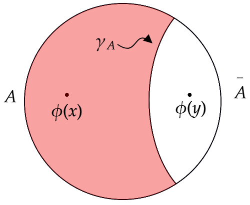
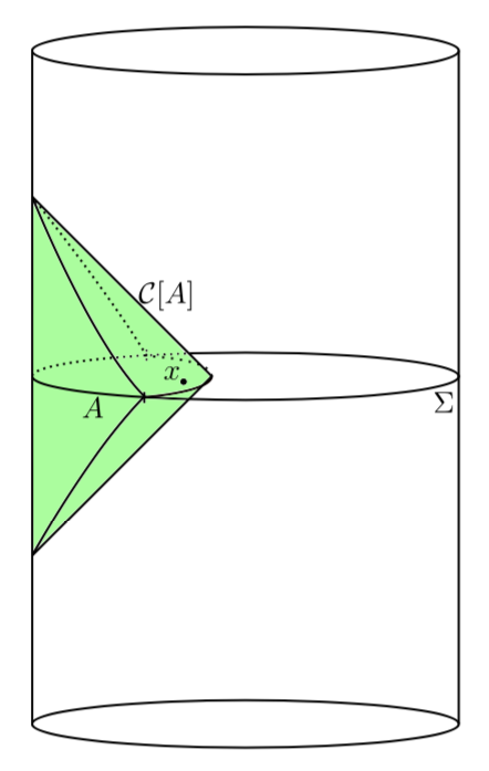
Figure 1 shows the conformal diagram of AdS space on the left and a constant time slice of this spacetime on the right. The surface divides the bulk geometry into two regions, thus also dividing the boundary into two regions labeled and . According to the Ryu-Takayanagi conjecture [8, 9] the entropy due to entanglement between the degrees of freedom living in with those living in is given by the area of the surface dividing the bulk interior:
| (1) |
where is the number of spatial dimensions of the bulk AdS geometry.
The same time slice is shown in Figure 2. The bulk is divided into two regions, now labeled and , with the dividing surface labeled . Now, imagine shrinking the surface so that its area gradually decreases. As the area of this surface reduces, the Ryu-Takayanagi formula tells us that the entropy of entanglement, between the degrees of freedom living on the boundary of region and those living on the boundary of region , also starts to reduce. Geometrically, the effect of shrinking is to reduce the connectivity between the bulk regions and as shown on the right side of Figure 2. When the area of goes to zero, the two regions will become completely disconnected. At the same time the entropy of entanglement between the degrees of freedom living on the boundary of region with those living on the boundary of region will also vanish.
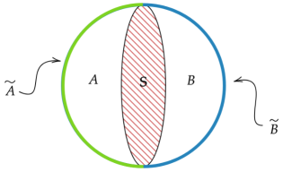
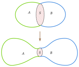
This simple thought experiment was first proposed in 2010 by Mark Van Raamsdonk [10]. It illustrates in a very simple yet dramatic manner how the RT formula, in conjunction with the AdS/CFT conjecture provides a straightforward description of how classical spacetime can emerge from entanglement between degrees of freedom of some underlying quantum field theory. It provides a very simple, yet physically plausible explanation for how different pieces of a spacetime can be “sewn” together to build a macroscopic geometry.
1.1 AdS/CFT Bulk Reconstruction
Further background for the problem requires us to use slightly more technical language. The metric for asymptotically Anti-deSitter spacetimes (AdS) is generally expressed in terms of the time-like co-ordinate , a “radial” co-ordinate and a set of co-ordinates which describe the spatial dimensions orthogonal or transverse to : . Using the global co-ordinates, the metric can be expressed as:
| (2) |
where is the AdS radius. This metric is a solution to the vacuum Einstein equations with a negative cosmological constant , given by: , where is the total number of spacetime dimensions. In the AdS/CFT correspondence one usually talks about spacetimes which are only asymptotically AdS, i.e. whose metric can be written in the form:
| (3) |
where for large enough. The boundary of the spacetime is located at .
Consider some asymptotically AdS spacetime , with boundary . The bulk geometry of satisfies the Einstein field equations. Consider some fields living on a constant time slice of . In terms of these quantities the AdS/CFT conjecture can be stated mathematically in terms of the following expression, known as the Gubser-Klebanov-Polyakov-Witten (GKP-Witten) relation [11, 12]:
| (4) |
where is the gravitational action evaluated in the bulk for a given field configuration ; is the value of the fields evaluated only on the boundary and is some operator acting on the on the Hilbert space of the boundary field theory. This relation can be understood as the statement that:
Proposition I: classical expectation values of bulk fields in asymptotically anti-deSitter spacetimes can be calculated in terms of quantum expectation values of operators acting on the Hilbert space of the boundary field theory
There is, however, a caveat which prevents us from constructing a one-to-one correspondence of the physics in the boundary with the physics in the bulk. This is because the equality (4) holds only asymptotically as . The question that therefore presents itself is: can we reconstruct bulk fields (for ) from knowledge of boundary fields?
It turns out that bulk fields, i.e. with , can indeed be reconstructed from boundary operators [13]. For this purpose it is helpful to work in the Poincare co-ordinates for AdS:
| (5) |
where now the radial co-ordinate is and the boundary lies at . In these coordinates, on a constant time-slice, a bulk field with normalizable fall-off near the boundary can be written as:
| (6) |
In terms of these co-ordinates, the value of the field at a point in the bulk can be expressed in terms of the boundary field via:
| (7) |
where is the kernel or the smearing function. corresponds to a local operator in the CFT:
| (8) |
This relationship implies that local bulk fields are dual to non-local boundary operators:
| (9) |
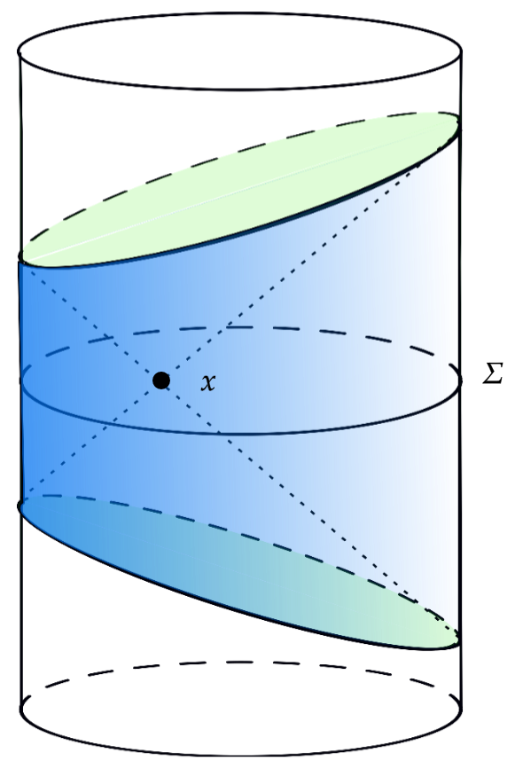
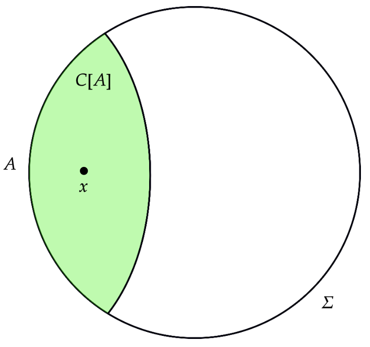
where the integral has support over a subset of points on the boundaryConsider a spatial surface which is a constant time slice of the AdS cylinder as shown in 3(a). Then the integral in (9) has support on the subset of the boundary shaded in green, i.e. all the points on the boundary which are at a spacelike separation from the bulk point . This construction can be further restricted [14, 15, 16] to limit the domain of integration to the portion of the boundary which lies in the “causal wedge” of . This is the boundary region shaded in green shown in 3(b). Here is a subset of the spatial slice , such that the bulk point lies in the region enclosed by and the Ryu-Takayanagi surface corresponding to as shown in 3(c).
1.2 Redundancy in Bulk Reconstruction
It now becomes apparent that there is a redundancy in this description of bulk reconstruction. Consider for instance a second region lying on the boundary of , which has non-zero overlap with as shown in 4(a), such that the bulk point lies within the causal wedges of both and . According to the HRT prescription for bulk reconstruction, fields at the bulk point can be mapped either to an operator with support only in , or to an operator with support only in the region .
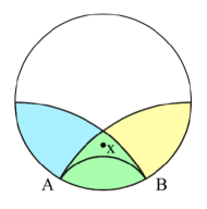
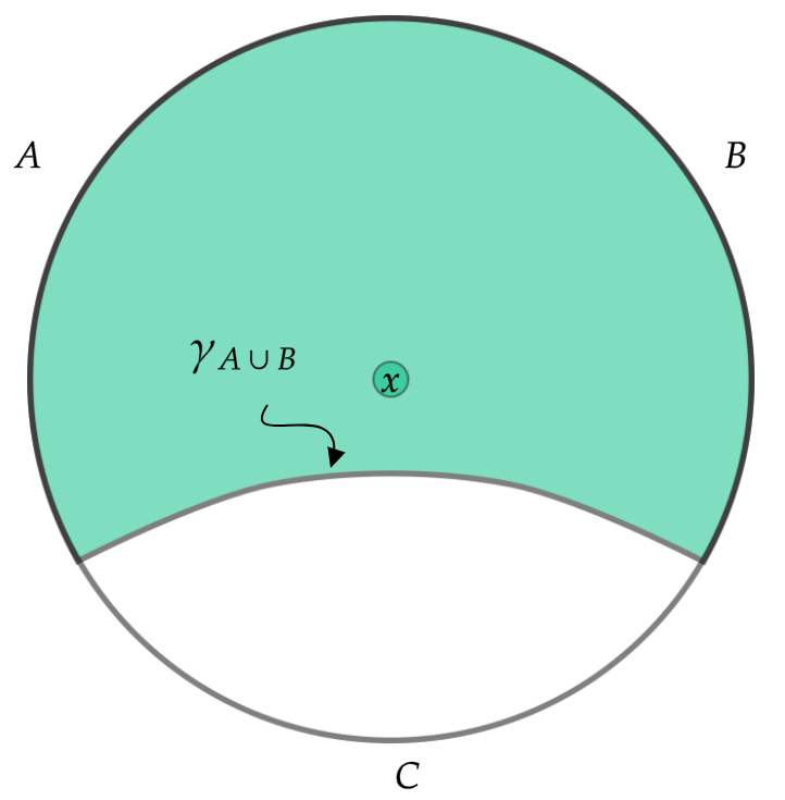
Now consider the boundary segment which consists of the intersection . The associated causal wedge does not contain the point , even though as is clear, the bulk point does fall within the intersection of the causal wedges of and . In order for there to be a unique description of the bulk fields in terms of boundary operators we require that:
| (10) |
For this to be true, both operators must have support only in . However, as just noted the causal wedge of this region does not contain the bulk point and therefore any CFT operators with support only on cannot provide a faithful representation of bulk fields at . The only conclusion one can arrive at is that:
| (11) |
Since both operators separately encode the physics near the same bulk point and the fact that the two operators cannot be the same, leads us to conclude that [4]:
Proposition II: There does not exist any unique representation of bulk fields in terms of CFT operators living on (some subset of) the boundary.
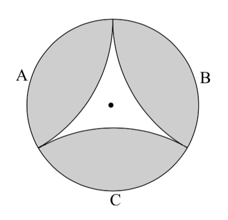
We can shed more light on the nature of this redundancy by considering three segments of the boundary as shown in 4(b). As can be seen the bulk point (in the center) does not lie within the causal wedges (shaded in grey) of either of the three regions or . Therefore we do not expect to have a representation of bulk fields at the given point to have a representation in terms of operators defined solely on either one of the three regions. Now consider, the third figure 4(c). From this we can see that the bulk point now lies in the causal wedge of the regions , and , taken separately. Consequently there exists a representation of the bulk fields in terms of operators:
As Almiehri et. al. point out in [4] this sort of dependence of the bulk fields on three different operators defined on overlapping boundary regions is reminiscent of the three-qutrit quantum error correcting code wherein one “logical” qutrit is encoded in terms of three “physical” qutrits. At this stage, let us rapidly overview the basic ideas behind quantum error correcting codes and the three-qutrit code in particular.
2 Quantum Error Correction
In any computation, quantum or classical, errors are inevitable. “Error correction” protocols [17, 18] allow us to correct (non-catastrophic) errors. The basic idea behind all error correction protocols, whether classical or quantum, is to encode the “logical” degrees of freedom - which carry the information we would like to protect from errors - in terms of some “physical” degrees of freedom. The number of physical d.o.f is necessarily larger than the number of logical d.o.f. The simplest example of such a scheme is the repetition code, for either classical or quantum information, in which a single physical d.o.f is encoded in two or more logical d.o.f in the following manner:
| (12) |
where symbols with a on top represent logical qubits and those without it are physical qubits. Here we have encoded one logical cbit/qubit in three physical cbits/qubits. Let us assume that the errors in our system will only flip one of the physical cbits/qubits in a single code-word, e.g. . Such errors can therefore be corrected by using the majority rule. Those cbits/qubits which are greater in number are the “correct” ones and those which are in the minority are the “wrong” ones. Thus would become after correction and would become . Of course, if the errors cause more than one cbit/qubit to flip then this simple scheme would no longer be effective.
The basic principle behind all forms of error correction is safety through redundancy.
Definition: A quantum error correcting code consists of a triple [19]:
| (13) |
where: is the “code space”, dimensional subspace of a higher dimensional “physical” Hilbert space ; is a set of quantum operations on which generate errors; and is a set of quantum operations on which can “undo” the errors. denote, respectively, the dimensions of the physical Hilbert space and the code subspace.
An example of such a code is Shor’s nine qubit code, where a single logical qubit is encoded using nine physical qubits.
| (14) |
The fundamental ingredient in this code are the GHZ (Greenberger-Horne-Zeilinger) states111These states are also sometimes referred to as “cat” states in honor of Schrodinger’s famous feline:
| (15) |
For future reference we reproduce below the quantum circuit which is used for generating GHZ states:
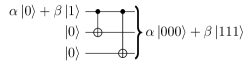
This circuit involves application of the CNOT gate to qubits and qubits in succession. The CNOT gate is shown below:

In the remainder of this paper we will show that the consideration of discrete symmetries of spin-networks - the kinematical states of quantum geometry in the framework of Loop Quantum Gravity - naturally leads us to discover the existence of topological excitations which correspond precisely to CNOT gates. These excitations can then be used to build GHZ states, or in combination with certain other single qubit gates - also represented in terms of operators acting on topological degrees of freedom - can be be used to generate an arbitrary quantum circuit.
3 Spin Networks and Quantum Geometry
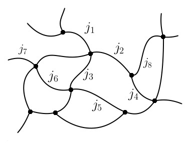
Loop Quantum Gravity - or “LQG” for short - is an approach222there are many introductory reviews on LQG, at various levels of technical sophistication ranging from advanced [20, 21, 22] to intermediate [23, 24, 25, 26] to (relatively speaking) elementary [27, 28, 29] towards building a non-perturbative theory of quantum gravity. LQG provides a description of quantum states of geometry in terms of objects known as “spin networks”. A spin-network is an arbitrary graph , whose edges are labeled by representations of (7(a)) and whose vertices are labeled by invariant tensors known as “intertwiners”. More simply, spin-networks are graphs whose edges carry angular momenta and whose vertices provide a means for adding together all the angular momenta coming into that vertex from its adjoining edges.
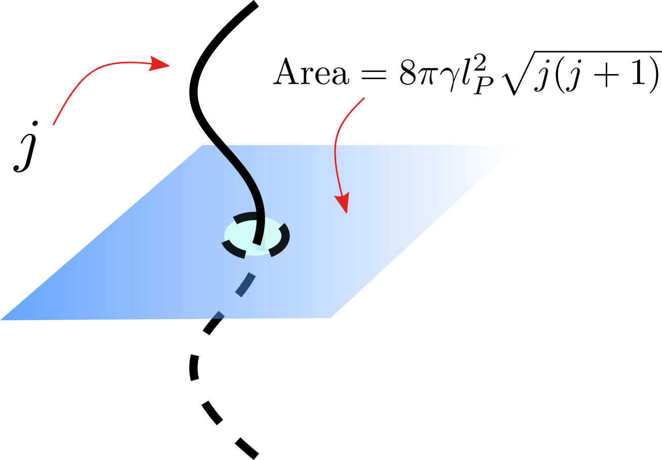
A spin-network defines a state of quantum geometry. With each edge we can associate a quantum of area and with each vertex a quantum of volume. 8(a) shows a single edge of a spin-network carrying an angular momentum , puncturing a surface (shaded in blue). This edge endows the surface with a quantum of area given by , where is the Planck length and is a free parameter known as the Barbero-Immirzi parameter. The particular value of will not be relevant for our purpose.
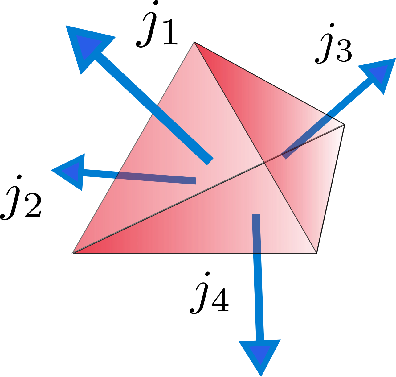
Spin network vertices are associated with quanta of volume. In 7(b) a single tetravalent vertex is “blown up”. Each edge adjoining the vertex carries an angular momentum . With each edge we can associate a triangle of area . The four triangles associated with the given vertex, will then close up333The four angular momenta must satisfy the closure condition . This is analogous to the requirement that a classical tetrahedron satisfies , where are the vectors normal to each face. to form a tetrahedron with which we can associate an operator whose eigenvalues can be interpreted as the volume of the resulting “quantum tetrahedron”. For more details we direct the interested reader to one of the several reviews listed in the references.
Spin networks provide a genuinely non-perturbative way to quantize classical geometry. A priori, there is no requirement for a background manifold with any sort of topological or geometric structure, in order to be able to define a quantum state of geometry. The only information required to specify a spin-network state is knowledge of the graph (i.e. the number of edges and vertices and their connectivity structure) and the labeling of edges and vertices by spins and intertwiners respectively:
| (16) |
where are the numbers of vertices and edges respectively in the graph, is the connectivity matrix, are the edge labels and are the vertex labels.
Now what makes these states bona-fide states of quantum geometry, rather than simply being an ad-hoc construction is the fact that these states are exact solutions of the ADM Hamiltonian. As is very well understood, in the formulation of general relativity, first presented by Arnowitt, Deser and Misner [30] Einstein’s equations can be expressed as a sum of constraints. When working in the connection formulation there are three constraints. These are known as the Gauss constraint , the vector or “diffeomorphism” constraint and the scalar or “Hamiltonian” constraint . In this language the problem of quantum gravity reduces to that of finding states which are annihilated by the quantum operator versions of all three constraints. It turns out that spin network states are annihilated by two of the constraints - the Gauss and diffeomorphism constraint. The Gauss constraint is the statement of invariance of the state under gauge transformations. This is satisfied by spin network states due to the closure condition: , i.e. the sum of angular momenta carried by all the edges adjoining a given vertex must give zero. The diffeomorphism constraint is trivially satisfied because the embedding of a graph in a smooth manifold does not affect its geometric content. One can move the edges and vertices of the graph around in the ambient manifold, but as long as the connectivity structure of the graph is unchanged, the spin network state is also unaffected.
The action of the third constraint - the Hamiltonian constraint - is expected to generate “time evolution” of the quantum geometry. The resulting states are known as “spin foams” and represent causal histories connecting two different spin network configurations. For our purposes we are interested only in spin-networks which represent the spatial geometry as a given instance of time.
4 Diffeomorphism Invariance of Spin Networks
The ADM constraints discussed in the last section fail to capture the full dynamics of general relativity. The reason for this is the existence of “large” diffeomorphisms (those which cannot be continuously deformed to the identity). This is completely analogous to the existence of topologically non-trivial solutions in field theory due to the existence of “large” gauge transformations. Diffeomorphisms constitute the gauge symmetry of general relativity. Therefore it is natural to consider not only small diffeomorphisms - those continously deformable to the identity - but also large diffeomorphisms - those which lie in the disconnected component of the gauge group. The ADM constraints only encode the small diffeomorphisms. As was discovered by Freidman and Sorkin in the 1980s [31], the consideration of large diffeomorphisms leads to manifolds which have half-integer spin.
In order to complete the description of spin network states as candidate states of quantum geometry, one has to consider the action of large diffeomorphisms in addition the small ones. Spin networks are trivially invariant under small (spatial) diffeomorphisms, because as explained in the previous section, moving edges or vertices around without changing the graph connectivity or spin labels does not change the geometric content of the state. Now, large diffeomorphisms would also not change the graph connectivity or the spin labels. Thus the questions arises as to what effect, if any, would such transformations have on spin networks? It is not hard to convince oneself that the effect of large diffeomorphisms would be to break and reconnect spin-network edges in such a way that the winding and linking numbers of those edges would change. Thus, while the graph structure and spin labels would remain intact, a spin-network with two of its edges “braided” around one another is a topologically distinct state from one which does not have such a braiding.
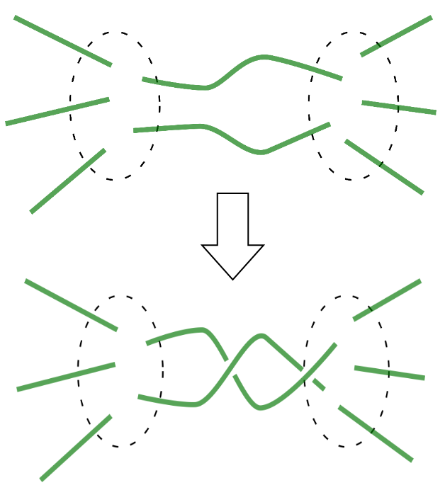
This is illustrated in Figure 9. The upper portion of the figure shows a generic spin network state with two edges connecting two different regions (whose boundary is drawn as the dotted curve) of the graph. The lower portion shows what happens to this graph under the action of a large diffeomorphism. The two edges break and reconnect after having wound around each other once. The resulting graph carries the same geometric information as the initial state but has a different topological structure.
If we wish to construct states of quantum geometry which incorporate the full dynamics of quantum general relativity, we must construct states which are invariant under both small and large diffeomorphisms.
5 Diffeomorphism Invariance and Yang-Baxter Equation
Now, in order to understand the effect of large diffeomorphisms on a quantum state of geometry, let us consider the two configurations depicted in figure Figure 10. There are two surfaces and with two edges (shown in green) connecting them. Now, as shown for e.g. in [32], we know that at the points where the edges punctures the surfaces we can associate the Hilbert space of a point particle. Let us denote the state of the two punctures on the first surface as , and on the second surface as , . On the left side of the figure the two edges are unbraided and on the right side they are wound once around each other.
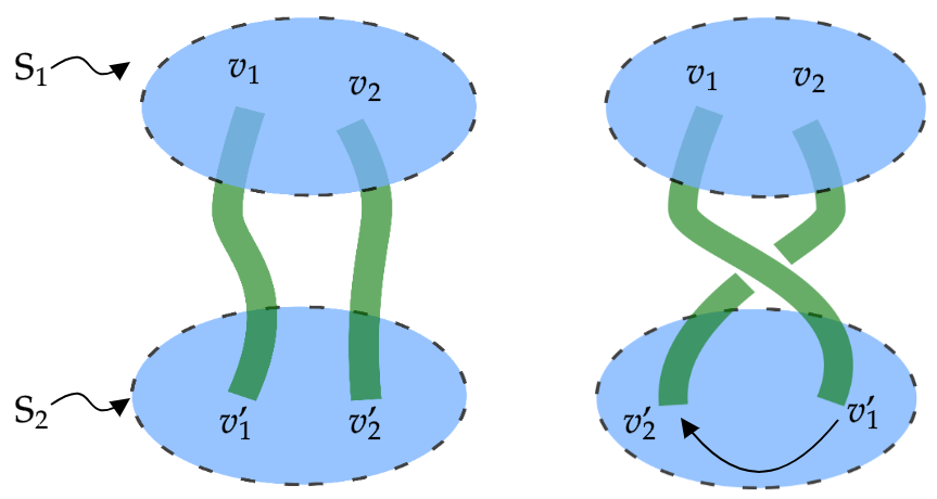
Let us denote the Hilbert space associated with the puncture as . Then the state of the two punctures, either on or on , resides in the tensor product Hilbert space: . On the right side of the figure we see that braided the edges around each other has the same effect as exchanging the two punctures on the second surface. Now, in general, when we exchange two particles in any quantum system the total state of the system undergoes a unitary transformation. In three spatial dimensions particle exchange can only leads to a change in the phase of the wavefunction by (for bosons) or for fermions. However, in two spatial dimensions one can have more complex behavior (see for e.g. [33]). The unitary operator associated with such an exchange need no longer be a trivial multiple of the identity.
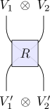
In general we would have the following relationship between the states of the two particles before and after exchange:
| (17) |
where is some unitary operator. Diagrammatically this is shown in the figure Figure 11.
The form of the unknown unitary is, as yet, undetermined. We can now use the fact that an arbitary spin-network state should be invariant under small diffeomorphisms to determine an exact equation which must be satisfied by any . Consider the two configurations shown in Figure 12. Now instead of two punctures, we are considering the case where each surface contains three punctures. The two figures might seem different, but they are not. It is easy to convince oneself that one can slide the middle thread in such a way as to go from the configuration on the right to the one of the left, without breaking or joining any threads. Such a transformation is nothing but a small diffeomorphism acting only on the middle thread!
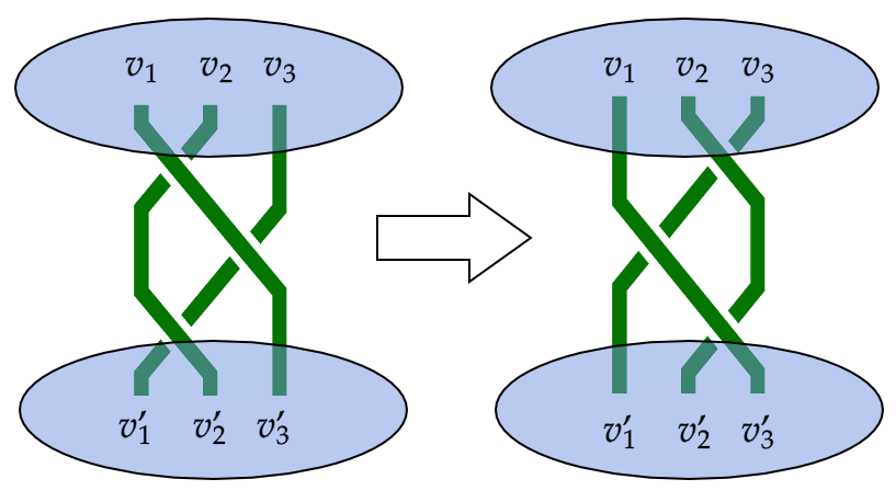
However, while topologically the two configurations appear to be the same, the order in which the pairwise unitary operator acts on the three-particle state is different in both cases. On the left we see that the, in the first step, first two threads are braided while the first in untouched. This operation on the three particle Hilbert space can be denoted by the operator , where the subscripts denote the particle on which the operation acts. The second step (on the left) can be represented as and the third one (on the left) is again . The full unitary operation corresponding to the left hand side of Figure 12 acting on the spin-network state can thus be expressed as:
| (18) |
In a similar way one can write the total unitary corresponding to the right hand side of Figure 12:
| (19) |
While the two unitary operations shown in (18) and (19) appear to be similar they are not the same. However, if we insist that the state of quantum geometry represented by the given spin network should be invariant under small diffeomorphisms then the two unitary operations must have the same effect on the state . This equivalence can formally be written as an operator equation:
| (20) |
We see here that the particular spin-network state in question factors out because this equation should hold for all spin-networks for the theory to be physically consistent, and we are finally left with just an operator equation. This equation is famous in the field of condensed matter and goes by the name of the Yang-Baxter equation [34] in honor of the two individuals most deeply associated with studying its solutions and recognizing its significance. It can be solved exactly to give us the exact form of the unitary operator . As we shall see in the next section the form of is precisely that of a CNOT gate - a two qubit gate which is universal for quantum computation.
6 Yang Baxter Equation and Quantum Computation
It turns out to be the case that the manipulations of spin-network edges described in the previous section are precisely the same operations as those used to perform quantum computation using topological phases of two-dimensional condensed matter systems as the computing “hardware”.
Let us assume for the time being that we can identify the Hilbert space of a puncture (c.f. Figure 10) with of a spin particle, i.e. a qubit. In this case the operator is a two qubit gate and can be expressed as a matrix. The exact solution for in this case is given by the following expression [35]:
|
|
(21) |
This operator acts of the state space of two qubits. The basis states of a single qubit can be written as . The basis states of a two qubit state can then be written as: . The operator given in (21) acts on this state space. The effect of this operator can be described the circuit diagram shown in Figure 6 which is repeated below for the reader’s convenience.

Now, it is a well known fact in classical computation that all of the gates used in Boolean logic - AND, OR, XOR, NAND and NOT - can be constructed given only the NAND gate. The NAND gate is thus said to be “universal” for classical computation. Similarly, using only a finite set of discrete two and one qubit gates one can construct any unitary operator to arbitrary precision [36, Ch. 4], by repeated application of the gates in the given set. One such set of universal gates consists of the CNOT gate, Hadamard gate, phase gate and the gate. Except for CNOT, the remaining gates all act on a single qubit. We list these gates below in the standard basis:
| (22a) | ||||
| (22b) | ||||
| (22c) | ||||
What we have discovered so far is that quantum diffeomorphism invariance of spin network states implies that these states naturally carry an implementation of the entangling two qubit CNOT gate. If, in addition, it would be possible to incorporate the gates mentioned in (22) as some additional structure in spin-network states, then it would imply that spin-network states are universal for quantum computation. Already the existence of the CNOT gate hidden within the state space of loop quantum gravity, tells us that there is a deep connection between quantum computation and quantum gravity, confirming what we already know from various other independent approaches [4, 5, 6, 7, 37] to the question of quantum gravity.
7 Framed Edges and Single Qubit Operators
It turns out that spin-networks can be endowed with additional topological structure in a natural manner and the degrees of freedom of this structure can then naturally be interpreted as the action of quantum gates acting on individual qubits. This structure turns out to be required due to two independent considerations. Let us explain these in turn.
In his famous paper [38] Witten was the first to point the deep connections between (topological) quantum field theory and knot theory. In particular he showed the the expectation value of the Wilson loop functional evaluated on any knotted curve in Yang-Mills theory in dimensions is related to the knot invariant of known as the Jones polynomial. In this work he showed that a crucial step in the calculation involved the calculation of the self-linking number of a knot. This quantity is ill-defined if the knots are taken to be one-dimensional curves. In order to “regularize” the associated integral one has to introduce a framing of the knot, i.e. replacing the one-dimensional curve constituting the knot with a two-dimensional ribbon.
The second justification for using framed ribbons rather than one-dimensional strings comes from Smolin’s seminal work [39] linking topological quantum field theory with the field of loop quantum gravity which was in its infancy at the time. By considering the action of certain Wilson loop operators acting on punctures between spin-network edges and an arbitrary two-dimensional surface he was able to deduce that the punctures, and thereby the spin network edges, would have to be endowed with a framing.
Taken together, these two lines of argument are enough to convince oneself that the full state of loop quantum gravity should incorporate braided ribbon spin networks rather than the one-dimensional versions commonly encountered in the literature.
The careful reader would have noticed that we have used such framed ribbons, rather than one-dimensional lines, to represent spin network edges in several of the figures in this paper. This is not only for aesthetic convenience but also because ultimately we wish to work with framed or ribbon spin networks.
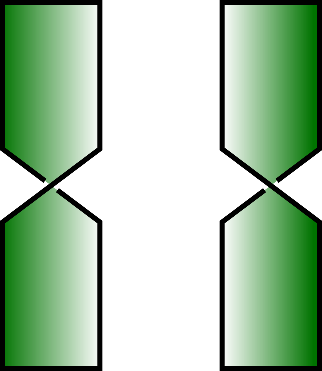
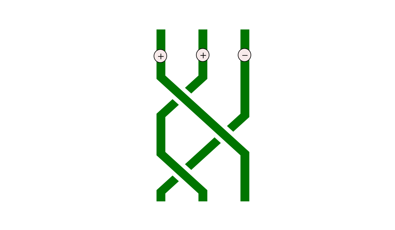
The moment we replace spin network edges with framed ribbons we realize that we have gained another topological degree of freedom in the form of twists which the ribbon can have. Let us assume that the simplest possible twist can be if one end of the ribbon is rotated degrees relative to the other edge in either a clockwise or counter-clockwise manner. can, in principle, take any value between and . Here, for simplicity, we will assume that can only take values . As we shall see later, this value also arises naturally when considering the application of discrete symmetries of spin-networks. 13(b) shows an example of a configuration with three ribbons, with the first two having a twist and third one with a twist. 13(c) shows how the twisting and braiding operations can be combined.
It is natural that, as was the case with braiding of two edges, putting a twist in a single framed edge should also correspond to the action of some unitary operator on the given edge. It is not clear at this stage precisely which form this unitary operator should take out of the one-qubit gates listed in (22): the Hadamard, phase or gates, or perhaps some other one qubit unitary. What is clear is that in addition to CNOT, the twisting operation will give us at least one additional single qubit unitary. If somehow we were able to identify additional topological degrees of freedom which could be associated with the three single qubit gates listed in (22) then we would be well placed to make the following proposition:
Proposition III: The set of framed, braided spin network states provides a complete set of states required for universal quantum computation.
which could alternatively be stated:
Proposition III’: The state space of loop quantum gravity is dense in the set of operators required for universal quantum computation.
We are now well placed to come to the central result of this work, which is the claim that the state space loop quantum gravity, extended by inclusion of braiding and twisting of framed edges, provides us with a source of generating GHZ states, which are a central resource for quantum error correcting codes. To do so we need only remind ourselves of the structure of the circuit which generates a GHZ state. This circuit is shown in Figure 5, which is reproduced below for the reader’s convenience.

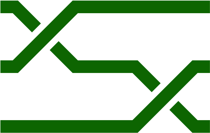
The interested reader can easily verify, using the explicit form of the operator given in (21) that the braid operation shown in 14(b) generates the GHZ state given that the first qubit starts in the state and the second and third qubits start in the state. The shown braid configuration then corresponds to the unitary operator .
8 Conclusion: Elementary Particles as Quantum Error Correcting Codes
In this work we have made the following observations. First, in order to consider the full state space of loop quantum gravity, knotting and braiding of spin-network edges needs to be taken in account. Second, the action of the operator version of small diffeomorphisms is given by the Yang-Baxter equation whose solutions yield a two qubit unitary gate which is universal for quantum computation. And, finally, the inclusion of topological degrees of freedom allows us to generate states which are essential ingredients in quantum error correcting codes.
It is also interesting to note that the braid configurations shown in 14(b) are identical to those in the groundbreaking work by Sundance Bilson-Thompson [40, 2] wherein he identified these states with leptons belonging to the first generation of the Standard Model of elementary particles.
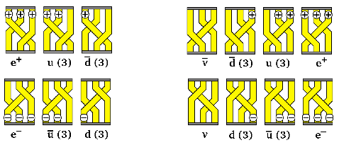
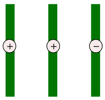
Considering all possible configurations of the elements of the braid group with three strands with twists, one ends up with the set of configurations shown in Figure 15. By making the assumption that the twist on a ribbon corresponds to an electric charge of to that ribbon, we are find that there are precisely four configurations with total charge , and each. There are two elements which are uncharged (without any twists on any of the ribbons). The charged elements can be identified with an electron (charge ), an up quark (charge ), down quark (charge ) and their antiparticles. After this assignment we are still left with two configurations for each value of the total charge. These two configurations are mirror reflections of each other. This motivates us to identify one set of these configurations with the left handed leptons and the other with right handed leptons . The two uncharged configurations form a particle-antiparticle pair (applying the operation of braid concatenation to the two configurations gives us the identity braid) and are identified with the neutrino () and the anti-neutrino ().
There is a certain elegance in associating elementary particles with elements of the code words of a quantum error correcting code. The vacuum is filled with fluctuating quantum fields. However, we don’t identify all of the possible fluctuations of the quantum vacuum with elementary particles. There is a certain element of stability that elementary particles possess. If we shoot an electron from one end of a long vacuum tube - from which the atmosphere has been evacuated - then, in the absence of any collisions with some stray particles passing by, we expect to find an electron arriving at the other end of the tube. This is true, even though the electron has to interact with the fluctuations of the quantum vacuum in its journey through the tube. In the language of error correction, such a state which is immune to fluctuations in its environment is known as a noiseless subsystem [41, 19]. It is precisely these noiseless subsystems which serve as the elements of the code space. It would only be natural if elementary particles were to be identified [42, 43] with the noiseless subsystems of any underlying quantum gravity theory.
It is important to note that several prior authors [2, 44, 45, 3, 46, 47] have focused on the role of ribbon spin networks in loop quantum gravity. However, to the best of our knowledge this work (and another prior paper by the author [1]) are the only ones to have made the association between ribbon networks, elementary particles and quantum error correcting codes.
In recent work Freidel and colloborators [48, 49] have suggested assigning a Kac-Moody algebra to the punctures where a spin network edge intersects a two-dimensional surface. They further argue that this implies that the edges of spin networks should be considered as tubes rather than as one dimensional curves. This sort of a structure was first suggested by the present author in a much older work [3] relying on arguments centered around discrete symmetries of spin networks. There might exist a direct link between the work of Freidel and co-workers and the present work. This is suggested by a close relation between solutions of the Yang Baxter equation and Kac-Moody algebras [50]. This, however, must be left for future works.
References
- [1] D. Vaid, Elementary particles as gates for universal quantum computation, June, 2013.
- [2] S. O. Bilson-Thompson, F. Markopoulou and L. Smolin, Quantum gravity and the standard model, Mar, 2006.
- [3] D. Vaid, Embedding the bilson-thompson model in an lqg-like framework, 1002.1462.
- [4] A. Almheiri, X. Dong and D. Harlow, Bulk locality and quantum error correction in ads/cft, .
- [5] E. Mintun, J. Polchinski and V. Rosenhaus, Bulk-Boundary Duality, Gauge Invariance, and Quantum Error Corrections, Physical Review Letters 115 (2015) , [1501.06577].
- [6] F. Pastawski, B. Yoshida, D. Harlow and J. Preskill, Holographic quantum error-correcting codes: Toy models for the bulk/boundary correspondence, .
- [7] B. Freivogel, R. A. Jefferson and L. Kabir, Precursors, gauge invariance, and quantum error correction in AdS/CFT, Journal of High Energy Physics 2016 (feb, 2016) , [1602.04811].
- [8] S. Ryu and T. Takayanagi, Aspects of holographic entanglement entropy, Journal of High Energy Physics 2006 (June, 2006) 045, [hep-th/0605073].
- [9] S. Ryu and T. Takayanagi, Holographic derivation of entanglement entropy from AdS/CFT, hep-th/0603001.
- [10] M. Van Raamsdonk, Building up spacetime with quantum entanglement, arXiv:1005.3035.
- [11] S. S. Gubser, I. R. Klebanov and A. M. Polyakov, Gauge theory correlators from Non-Critical string theory, hep-th/9802109.
- [12] E. Witten, Anti de sitter space and holography, hep-th/9802150.
- [13] A. Hamilton, D. Kabat, G. Lifschytz and D. A. Lowe, Holographic representation of local bulk operators, Phys.Rev.D74:066009,2006 (2006) .
- [14] R. Bousso, S. Leichenauer and V. Rosenhaus, Light-sheets and AdS/CFT, 1203.6619.
- [15] B. Czech, J. L. Karczmarek, F. Nogueira and M. Van Raamsdonk, The gravity dual of a density matrix, Classical and Quantum Gravity 29 (apr, 2012) , [1204.1330].
- [16] V. E. Hubeny and M. Rangamani, Causal holographic information, Journal of High Energy Physics 2012 (apr, 2012) , [1204.1698].
- [17] J. Kempe, Approaches to quantum error correction, Dec., 2006.
- [18] D. Gottesman, An introduction to quantum error correction and Fault-Tolerant quantum computation, 0904.2557.
- [19] D. Kribs, R. Laflamme and D. Poulin, Unified and generalized approach to quantum error correction, Physical Review Letters 94 (dec, 2005) , [0412076].
- [20] T. Thiemann, Introduction to Modern Canonical Quantum General Relativity, gr-qc/0110034.
- [21] T. Thiemann, Lectures on loop quantum gravity, Oct., 2002.
- [22] A. Ashtekar and J. Lewandowski, Background independent quantum gravity: a status report, Classical and Quantum Gravity 21 (2004) R53–R152.
- [23] S. Mercuri, Introduction to loop quantum gravity, 1001.1330.
- [24] P. Doná and S. Speziale, Introductory lectures to loop quantum gravity, 1007.0402.
- [25] G. Esposito, An introduction to quantum gravity, 1108.3269.
- [26] A. Ashtekar, Introduction to loop quantum gravity, 1201.4598.
- [27] D. Vaid and S. Bilson-Thompson, LQG for the Bewildered. Springer Nature, Feb., 2014, 10.1007/978-3-319-43184-0.
- [28] C. Rovelli, Zakopane lectures on loop gravity, 1102.3660.
- [29] C. Rovelli and F. Vidotto, Covariant Loop Quantum Gravity. Cambridge University Press, Cambridge, 2014, 10.1017/CBO9781107706910.
- [30] R. Arnowitt, S. Deser and C. W. Misner, The dynamics of general relativity, General Relativity and Gravitation 40 (May, 2004) 1997–2027, [gr-qc/0405109].
- [31] J. L. Friedman and R. D. Sorkin, Half-integral spin from quantum gravity, General Relativity and Gravitation 14 (July, 1982) 615–620.
- [32] A. Ghosh and D. Pranzetti, CFT/gravity correspondence on the isolated horizon, May, 2014.
- [33] J. Jain, Composite Fermions. Cambridge University Press, 1 ed., April, 2007.
- [34] R. J. Baxter, Exactly Solved Models in Statistical Mechanics. Dover Publications, Jan., 2008.
- [35] L. H. Kauffman and S. J. Lomonaco, Braiding operators are universal quantum gates, quant-ph/0401090.
- [36] M. A. Nielsen and I. L. Chuang, Quantum Computation and Quantum Information. Cambridge University Press, 1 ed., October, 2000.
- [37] D. Harlow, The Ryu–Takayanagi Formula from Quantum Error Correction, Communications in Mathematical Physics 354 (jul, 2017) 865–912, [1607.03901].
- [38] E. Witten, Quantum field theory and the jones polynomial, Communications in Mathematical Physics 121 (Sept., 1989) 351–399.
- [39] L. Smolin, Linking topological quantum field theory and nonperturbative quantum gravity, Journal of Mathematical Physics 36 (1995) 6417–6455.
- [40] S. O. Bilson-Thompson, A topological model of composite preons, arXiv preprint hep-ph/0503213 (mar, 2005) 6, [0503213].
- [41] P. Zanardi and M. Rasetti, Noiseless quantum codes, Physical Review Letters 79 (Oct, 1997) 3306–3309.
- [42] D. W. Kribs and F. Markopoulou, Geometry from quantum particles, gr-qc/0510052.
- [43] T. Konopka and F. Markopoulou, Constrained mechanics and noiseless subsystems, gr-qc/0601028.
- [44] Y. Wan, On braid excitations in quantum gravity, 0710.1312.
- [45] Y. Wan, Effective theory of braid excitations of quantum geometry in terms of feynman diagrams, 0809.4464.
- [46] J. Hackett, Invariants of braided ribbon networks, June, 2011.
- [47] J. Hackett, Invariants of spin networks from braided ribbon networks, 1106.5095.
- [48] L. Freidel, A. Perez and D. Pranzetti, Loop gravity string, Physical Review D 95 (nov, 2017) , [1611.03668].
- [49] L. Freidel, E. R. Livine and D. Pranzetti, Gravitational edge modes: From Kac-Moody charges to Poincar’e networks, 1906.07876.
- [50] H. J. deVega, Integrable quantum field theories, {Y}ang-{B}axter, {K}ac-{M}oody algebras and their links, in Proceedings of the 14th {ICGTMP} ({S}eoul, 1985), pp. 122–134, 1986, https://inspirehep.net/record/220098.