Variational quantum state preparation via quantum data buses
Abstract
We propose a variational quantum algorithm to prepare ground states of 1D lattice quantum Hamiltonians specifically tailored for programmable quantum devices where interactions among qubits are mediated by Quantum Data Buses (QDB). For trapped ions with the axial Center-Of-Mass (COM) vibrational mode as single QDB, our scheme uses resonant sideband optical pulses as resource operations, which are potentially faster than off-resonant couplings and thus less prone to decoherence. The disentangling of the QDB from the qubits by the end of the state preparation comes as a byproduct of the variational optimization. We numerically simulate the ground state preparation for the Su-Schrieffer-Heeger model in ions and show that our strategy is scalable while being tolerant to finite temperatures of the COM mode.
1 Introduction
Realizing many-body quantum states on quantum devices offers an experimental pathway for studying the equilibrium properties of interacting lattice models [1, 2, 3], quench dynamics [4, 5, 6, 7], or it can be viewed as a quantum resource, e.g., for sensing [8, 9, 10, 11]. Adiabatic state preparation has been experimentally demonstrated, e.g., on trapped ions [12] and atoms in optical tweezers [13]. However, this strategy is currently limited by the finite coherence times of quantum devices, incompatible with the long annealing times required by the adiabatic criterion [14]. An alternative, promising pathway towards quantum ground state preparation is given by feedback-loop quantum algorithms, and especially by the Variational Quantum Eigensolver [15, 16, 17, 18, 19, 20, 21] (VQE). In VQE, parametrized generally non-universal quantum resource operations, available on a given quantum device, are arranged in a variational sequence, or circuit ansatz, to generate entangled trial states. The trial states approximate a target ground state as a result of a closed-loop optimization of the variational parameters, where an energy cost function is minimized.
For trapped ion qubits, VQE was recently demonstrated using as entangling resource either the Mølmer-Sørensen gate [22], or a programmable analog quantum simulator of the long-range XY spin model [23]. Both these entangling resources generate effective interactions between ion qubits by coupling them to vibrational modes (phonons). Implementing the optical couplings off-resonantly, one effectively achieves robustness of these resource operations to the temperatures of the phonon modes. However, this strategy yields relatively slow rates [24, 25], limiting the performance of VQE, as the quantum processing suffers from decoherence.
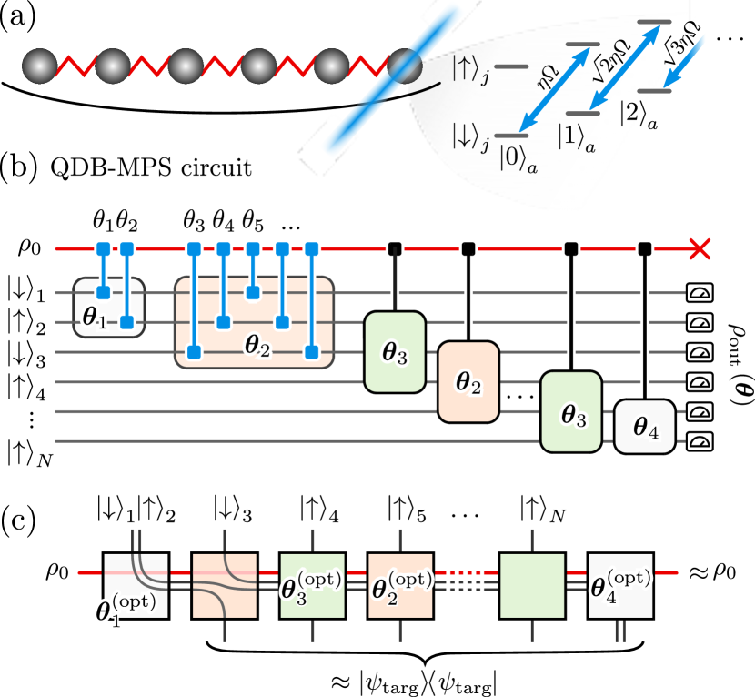
Here we propose a strategy to improve the efficiency of VQE on programmable quantum devices where interaction between qubits is mediated by auxiliary degrees of freedoms: Quantum Data Buses (QDBs). This strategy employs interactions between qubits and QDBs, naturally available in these devices, as variational resource operations in the quantum algorithm. We illustrate our approach on trapped ions, using the acoustic Center-Of-Mass (COM) phonon mode the axial vibrational mode where all ions oscillate in phase acting as a single QDB. We employ resonant optical coupling of ion qubits with the COM mode, yielding faster rates than off-resonant strategies, and thus being less prone to decoherence. Unlike logical gates designed with the resonant coupling, such as the C-phase gate [26], our variational approach is tolerant to finite temperatures of the COM mode, which do not limit the state preparation fidelity. Moreover, our strategy does not require to disentangle the QDB after each resource operation, but only at the end of the state preparation, ultimately yielding faster processing. The task of disentangling the QDB from the qubits is carried out by the optimization algorithm itself: As the output qubit state approaches the unique ground state of a target non-degenerate Hamiltonian, the QDB becomes disentangled without ever being measured.
Via numerical simulations, we investigate the scaling and robustness properties of our strategy for 1D lattice models. As a benchmark goal, we aim to variationally prepare the ground state, , of the Su-Schrieffer-Heeger (SSH) Hamiltonian [27, 28, 29] on ion qubits in a linear trap. Using only blue-detuned sideband optical pulses [30] as resource operations, we design the variational circuit ansatz shown in Fig. 1, which can efficiently realize Matrix Product States (MPS), a class of tailored variational wavefunctions capable of accurately capturing the equilibrium physics of many-body quantum systems in 1D [31, 32]. This ‘QDB-MPS circuit’ can incorporate various symmetries of the target model for enhanced performance, including approximate translational invariance in the bulk. In this paper, we will show that our approach is scalable, as we can approximate 1D ground states at saturating precision in the system size , without increasing the number of variational parameters [see Fig. 2(a)]. Additionally, we compare the results from the QDB-MPS circuit with other VQE strategies, still designed for trapped ion hardware, but using different sets of (coherent) entangling resources: (i) site-filtered Mølmer-Sørensen gates (ii) an analog quantum simulator of a long-range XXZ model [23]. We evaluate the respective accuracies in terms of various figures of merit, including excitation energy, fidelity, and two-point correlations. We demonstrate that our strategy can realize highly-accurate ground states even for QDB initialized at finite temperatures. Finally, we show that the QDB-MPS circuit can be up-scaled beyond the single-trap limit by being implemented in modular ion traps [33, 34]. Overall, we consider our strategy a viable, efficient route towards quantum state preparation in ion traps as well as in other quantum platforms that rely on QDBs, such as atom qubits coupled via photons in waveguides [35, 36] or cavities [37, 38, 39, 40], or superconducting qubits coupled by microwave resonators [41, 42, 43, 44].
The paper is organized as follows. In section 2, we describe the ion trap resource operations which we employ in the QDB-MPS circuit. We also review the resources used by other VQE strategies in ion traps, which we consider for comparison. We briefly introduce the target SSH model in section 3, and we discuss in detail the VQE strategies. We exhibit the results of our numerical simulation in section 4. Finally, in section 5, we summarize our conclusions and argue future perspectives for our approach.
2 Quantum resources in trapped ions
We consider a setup of ions in a linear Paul trap as a relevant quantum platform. The system qubit, or spin 1/2, at site is encoded by two internal electronic levels of ion [30], labeled and . Each ion, driven by laser fields in the transition between levels , experiences a recoil associated with absorption or emission of photons. This mechanism couples the internal ion levels with vibrational (phonon) modes, either axial or radial, depending on the optical setup [30], and allows phonons to be used as bosonic QDBs for the ion qubits. In ion traps, as well as in other quantum hardware using QDBs [45, 35, 36, 37, 38, 39, 40, 41, 42, 43, 46], various strategies have been developed to construct entangling quantum operations between qubits, while ensuring that the QDBs are disentangled from the qubits by the end of each operation. In what follows, we review some of these strategies.
Resonant Sideband Resources One possible approach to exploit QDBs in quantum hardware is to transfer information from one qubit to another by populating QDBs with real excitations [26, 46, 45, 43, 42]. In trapped-ion quantum computers, a typical choice is to elect the axial COM mode as single QDB, thanks to notable advantages: The mode frequency is well separated from the other phonon modes thanks to the linear dispersion at of the acoustic band, and additionally the qubit-phonon coupling is (roughly) homogeneous along the chain. Using focused beams, each individual ion can be coupled to the COM mode, usually via sideband optical pulses [26] implemented in the Lamb-Dicke regime [30] (where the Lamb-Dicke parameter is small, ). These pulses have frequencies detuned from the atomic transition exactly by the frequency of the COM mode . For the case considered further in this paper, it is sufficient to consider a single resonant sideband, either the negative detuned (red sideband) or the positive detuned (blue sideband). As the two choices lead to equivalent results, here we only illustrate the blue sideband case for simplicity, which is described by the Anti-Jaynes-Cummings Hamiltonian
| (1) |
addressing ion , where is the Rabi frequency, and achievable rates are of the order [47, 48]. In this picture, is the destruction operator for the COM mode, and is the lowering operator for ion . In Eq. (1), we used a gauge transformation to highlight the anti-unitary symmetry in the interaction Hamiltonian.
In Ref. [26], it was proposed to use resonant sideband pulses to realize the C-phase gate in ion traps. However, the main hindrance in using gates built out of resonant interactions with a bosonic QDB, as Eq. (1), is the requirement for the QDB to be perfectly initialized in a pure state, typically the vacuum , where index refers to the QDB mode. This requirement stems from the incommensurate rates of the transitions , depending on the number of excitations stored in the QDB, as highlighted in Fig. 1(a). As a result, the gate fidelity of resonant sideband gates in ion traps decreases roughly linearly with temperature of the initial thermal state (in units of ) of the COM mode.
Off-Resonant Sideband Resources To address this hindrance, alternative strategies to realize entangling operations were developed, in which couplings of the qubits to QDBs are implemented off-resonantly, and the QDBs are only virtually populated [49, 50, 51, 52, 39]. A prototypical example in ion traps, the Mølmer-Sørensen (MS) gate [49], can be implemented by coupling a subset of ions to the COM mode by a bichromatic laser beam with two frequencies, detuned from the qubit frequency by with . The resulting Hamiltonian
| (2) |
is an all-to-all interaction among qubits in , with . The condition [53] ensures that the qubits interact with each other via second-order processes, populating the COM mode only virtually and keeping it disentangled from the qubits. This approach is insensitive to the temperature of the COM mode. However, its rates are intrinsically lower than the rates of the resonant sideband resources (1), .
Analog Spin-model Resource Recent experiment [23] showed that VQE in ion traps can also employ a programmable analog quantum simulator as entangling resource operation. Such analog quantum simulator is realized by using a bichromatic laser beam that off-resonantly couples all the ions to all the transverse phonon modes, ultimately implementing the XY Hamiltonian [50, 54]
| (3) |
with power-law long-range couplings, where are the Pauli operators acting on qubit and is a uniform magnetic field. Thanks to the off-resonant couplings, the interaction (3) is also insensitive to the temperature of the phonon modes. However, typical rates [24, 25] are, again, much slower than the rates of resonant sideband interactions (1).
3 Variational Quantum Eigensolvers
VQE enables the experimental realization of ground states of arbitrary Hamiltonians, providing the best approximation for the given resource operations. Once the optimization is converged, the optimal quantum state can then be re-prepared on demand. For example, this state can be used as a resource to initialize the system for digital quantum simulation [55], which was recently demonstrated on ion traps in the context of lattice gauge theories [6].
Target model: Su-Schrieffer-Heeger As an example, in this work, we consider VQE for the ground state preparation of the SSH model on ion qubits. The SSH is an exactly solvable Hamiltonian [27, 28, 29], and a free-fermion prototype for symmetry-protected topological order in 1D, which reads
| (4) |
in open boundary conditions. is real in the canonical basis, exhibits -magnetization symmetry , and has zero-magnetization ground states with real amplitudes. We added a small staggered magnetic field at the boundaries, to lift the four-fold degeneracy arising in the topological phase (). With this prescription, is also CP symmetric (invariant under global spin-flip plus spatial reflection), translationally invariant in the bulk with a period of two sites, and has a critical point at .
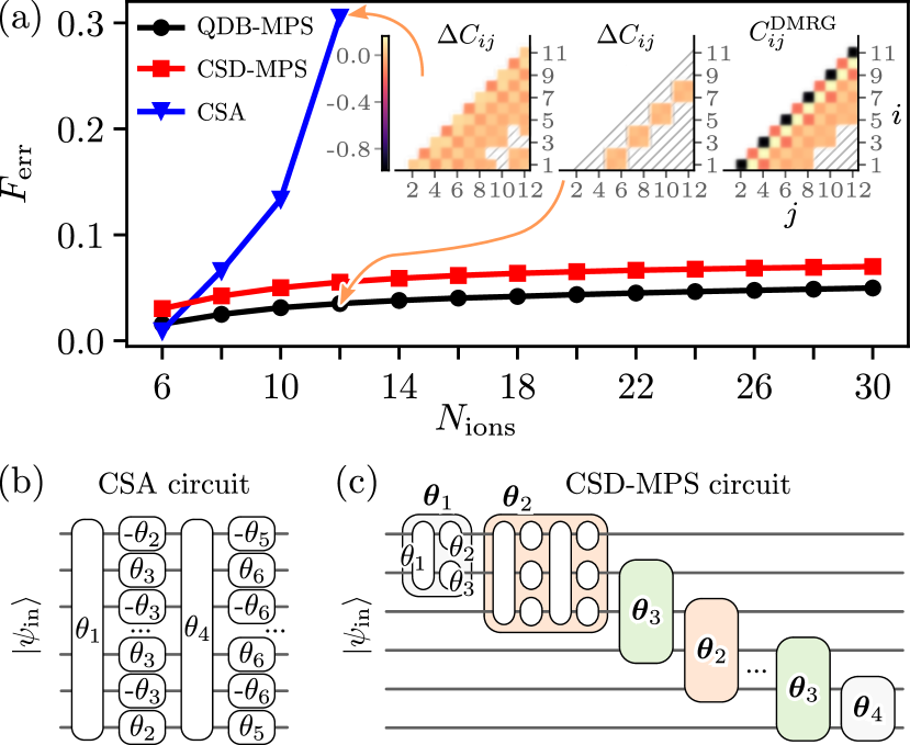
VQE with Closed System Analog resources (CSA) In Ref. [23], VQE was performed on trapped ions using Closed-System programmable Analog resources as in Eq. (3). We report the variational circuit ansatz considered in that work in Fig 2(b). This circuit alternates global resource operations, generated by , and single-qubit rotations . It was shown that this strategy is potentially scalable and capable of approximating ground states of 1D lattice models, including lattice gauge theories, with high fidelity. Here, we consider the CSA circuit as a comparison benchmark for the QDB-MPS circuit in preparing of the ground state of . We briefly review some details of the CSA strategy to highlight the differences with respect to the QDB-MPS.
The variational CSA circuit built with closed-system resource interactions generates (ideally pure) trial states
| (5) |
where the product of operators is ordered right-to-left for increasing . The system qubits are initialized in a Néel product state which can be prepared with high fidelity. For each given set of trial parameters , multiple instances of are prepared, and projectively measured in various local bases to reconstruct the energy cost function from one- and two-point correlation functions , . The cost function , function of , is evaluated at finite precision and minimized with a search algorithm capable of taking into account statistical errors. Upon convergence, reaches its global minimum, and the optimal set of parameters can be used to re-prepare the (approximate) non-degenerate ground state on demand.
Convergence of the search algorithm can be enhanced by incorporating symmetries of the target model in the trial states. For the CSA circuit, the zero -magnetization of the initial Néel state is protected both by the entangler and rotations . CP symmetry is protected by , and can be enforced on single-qubit transformation ‘layers’ by using correlated rotations angles . can be approximated as well, by repeating odd-site and even-site rotation angles, , away from the system edges [23].
While VQE provides the best approximate state preparation for a given set of resources in the presence of actual imperfections and noise [10], it is still affected by decoherence. By considering a different VQE circuit ansatz for trapped ions, which uses the high-rate resonant sideband resources of Eq. (1), we aim to tackle decoherence by speeding-up the preparation of trial states.
VQE with Quantum Data Buses (QDB-MPS) We design a variational circuit ansatz built on ion-COM mode interaction pulses (1), according to Fig. 1(b). Since now the COM mode becomes entangled to the ion qubits, the state of the qubits is generally mixed, both during the processing and in the output trial state
| (6) |
Parameters can be controlled by the duration of the sideband laser pulses. Similar to the closed-system case, the cost function is reconstructed from correlation functions evaluated on the trial qubit state, while the output state of the COM mode is discarded. As is minimized to approach the ground energy, approximates the unique, pure ground state , and the output state of the COM mode becomes automatically disentangled.
In our design, resource operations are arranged such that the circuit ultimately generates a variational Matrix Product State (MPS). In fact, MPS efficiently approximate ground states of 1D quantum lattice Hamiltonians, including the SSH model [56, 57]. In contrast to CSA resources, which are inherently global, blue-sideband operations (1) offer single-site addressability. This property allows us to progressively tailor the MPS from one edge to the other, as shown by the Tensor Network diagram [56, 57] in Fig. 1(c), in analogy to quantum circuits developed in the context of quantum machine learning [58]. Previous strategies for realizing MPS on quantum devices were proposed, both for deterministic state preparation [59, 60], as well as for variational state preparation [61] which employed long-range interactions. In contrast, our variational circuit requires only local ion-phonon interactions, and, therefore, can be up-scaled to modular ion trap architectures (see next section). Additionally, we introduce an approximate bulk-translational invariance to the ansatz, to reduce its variational complexity: In our circuit, interactions in the bulk can be virtually grouped in ‘boxes’ (drawn in Fig. 1(b) as grey rectangles at the edges, and orange and green for the bulk). Each box is defined by a set of variational parameters, which are repeated in the bulk boxes of the same color. At the same time, the maximum achievable bond dimension of the generated MPS can be controlled by increasing the size of the bulk boxes (see Appendix A). Figure 1 shows a specific design of the bulk boxes using five operations per box. Numerical results suggest that the number of operations per box is crucial towards the accuracy of the ansatz, while the ordering is marginal (data not shown). Appendix E illustrates our basic strategy to arrange operations inside a box.
As in the CSA case, we again incorporate symmetries of the target model in the trial states. First of all, since is fully imaginary, the operation is real as well as and , and, thus, the generated states have real amplitudes. Moreover, operations (1) protect an ‘extended’ magnetization symmetry , forcing the output qubits state to have well-defined -magnetization upon qubits and QDB becoming variationally disentangled (see Appendix B for details). We have analytically verified that, in the theoretical limit of infinite-depth circuits, the resources given by Eq. (1) are sufficient to generate ground states of any real, magnetization conserving Hamiltonian (proof in Appendix C). Controllability for an arbitrary lattice model (e.g., without symmetries) can be achieved by adding to the resources a resonant carrier operation for at least one ion.
We stress that resources of the form (1) are typical in various experimental platforms with bosonic QDBs, such as superconducting qubits connected via a resonator [46, 42, 43]. As such, the numerical analysis presented below can be generalized to these platforms.
CSD-MPS Circuit Ansatz We also compare our QDB-based approach with a variational MPS circuit ansatz realized with Closed System Digital resource operations (CSD-MPS circuit), as presented in Fig 2(c). This circuit is built with single-qubit rotations and site-filtered MS gates (2) applied to a local set of ions. Such resource operations protect z-magnetization in the trial state.
4 Results
Performance We compare the performance of the variational circuits by numerically simulating VQE for preparation of the ground state of Hamiltonian (4) in the gapped phase with . Trial states are obtained by evolving the initial quantum state in terms of density matrixes. For the QDB-MPS circuit, we consider the COM mode to be prepared in a thermal state with realistic average number of excitations [62, 63]. Other sources of imperfections are not taken into account, and, therefore, in contrast to the QDB-MPS circuit, simulations of the CSA and CSD-MPS circuits are free of imperfections. We consider the theoretical limit of unlimited measurement budget [10, 23], i.e., the cost function is the exact expectation value . To optimize parameters , we use a gradient-based optimization algorithm (see Appendix D), which can be adapted for noisy cost functions [64, 65, 66]. We emphasize that we consider a low number of free variational parameters, , which enables global search methods, such as the dividing rectangles algorithm [67, 68], already adopted in VQE [23]. For the analog resource entangler , realistic values and [23] are used. Further details on the circuit ansätze and their simulation are given in Appendix E.
To assess the accuracy of the ground state preparation, we employ various figures of merit. Besides the fidelity and the excitation energy (defined later on), we also consider a correlation-based error function
| (7) |
calculated using (parallel) two-point correlators
| (8) |
Here is evaluated on the optimized state and is the exact correlator of obtained by DMRG method [69]. We consider this error function in Fig. 2(a), to show that the proposed QDB-MPS circuit is able to prepare states with saturating in at fixed number of variational parameters . In particular, the insets show that these states have correlations accurately capturing . By contrast, arising from the CSA circuit grows rapidly for this specific task, and the correlators decay slower than in . We argue that this follows from the necessity to variationally remove the strong (power-law) correlations established by the long-range interactions in (3) to recover the exponential decay of correlations in the ground state. Moreover, the SSH ground state exhibits considerable (short-range) entanglement dimerization, which in turn seems to favor quasi-local resource circuits over global resource circuits. While the results for CSD-MPS and QDB-MPS circuits given in Fig 2(a) are compatible, the QDB-MPS is realized with higher-rate operations, and, therefore, is expected to be less prone to decoherence.
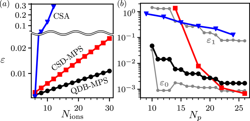
Scalability We study the scalability of the circuits in terms of the excitation energy in units of the energy gap, which bounds infidelity of the prepared states (Appendix F), and is thus a figure of accuracy. Here, and is the energy gap obtained by DMRG, which converges to a finite non-zero value in the thermodynamical limit since the target model is non-critical. Figure 3(a) shows that, for the QDB-MPS and CSD-MPS circuits, grows linearly with , in contrast to the CSA circuit. This is compatible with the previous observation that the two-point correlation functions carry, on average, an error saturating in , and the energy functional contains a linear amount of such correlators.
Scaling of the accuracy with , for the various methods and at fixed , is plotted in Fig. 3(b). Again, we observe that MPS circuits offer asymptotically better accuracy (or better parametric efficiency) than the CSA global resources. While increasing the number of parameters , we observe the CSD-MPS circuit reaches slightly better accuracies than the QDB-MPS circuit; we attribute this effect to the finite temperature of the COM mode we employed for the simulations. This argument is supported by the gray curves in Fig. 3(b), showing relative excitation energies obtained with the same QDB-MPS circuit and the same parameter values as the black plot but with different initial pure states of the COM mode for . For , we have , with . The plot shows that the two quantum trajectories are both variationally optimized in such a way that their error contributions are commensurate, .

Tolerance to temperature Here, we further investigate tolerance of the QDB-MPS approach to finite temperatures of the COM mode. As increases, more amplitudes are populated in , and, therefore, more equations need to be simultaneously satisfied, requiring higher to achieve the same accuracies. In Fig. 4, we consider the fidelity of the optimized output state of qubits, as a function of the average number of excitations and number of variational parameters . Panel (a) shows that, for fixed , decreases linearly with (similarly to the C-phase gate [26] built with sidebands), but with a slope that flattens for increasing . Therefore, to achieve a fidelity threshold, must be increased with . Remarkably, for the case under consideration, it seems that the required to obtain a static fidelity threshold scales logarithmically with . This behavior is illustrated in panel (b), where the density plot shows the infidelity of the optimized state as a function of and . The red curve highlights a fixed fidelity threshold . This property sets our QDB-based VQE apart from the approaches using sideband interactions to construct logical gates [26], in which imperfect cooling imposes a hard bound on the attainable accuracies.
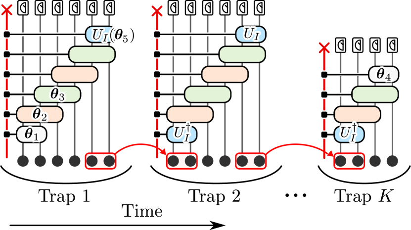
Scalability on a modular ion trap architectures The proposed QDB-MPS circuit 1(a) relies on interactions between individual ions and the COM mode. However, the number of ions which can be coupled to the COM mode in a single trap is limited by [34]. To further scale the ion trap quantum processors, modular ion trap architectures were proposed [33, 34]. Following these proposals, we describe ground state preparation with QDB-MPS circuit across multiple traps, as shown in Fig. 5. We consider coherent shuttling of few ions [33, 70] (or their internal states [34]) as a quantum communication channel among the traps, and we assume it to be error-free. We consider each trap containing a small number of ions, such that each ion is addressable via blue sideband pulses, realizing interactions as Eq. (1) with the COM mode of the corresponding trap. For simplicity, we assume that the initial thermal states, , of the COM modes are identical in each trap, as well as and their effective coupling to the ions.
The variational circuit ansatz is constructed sequentially along the network of traps, i.e., by applying operations in trap after all operations in trap are completed. Since each trap has an independent COM mode as a bosonic QDB, we introduce a variational ‘interface’ operation , constructed with resource interactions (1), which is applied to a set of ions (with the size of the bulk boxes) as the last operation for trap . This operation can be optimized in order to disentangle the COM mode of trap , effectively implementing , with the common state of ions and the COM mode. After transferring the set of ions to trap , we apply the unitary to the same ions plus the COM mode of trap prepared in state , effectively reconstructing the state . Ultimately, this operation removed the ‘impurity’ introduced by the interface between the two traps.
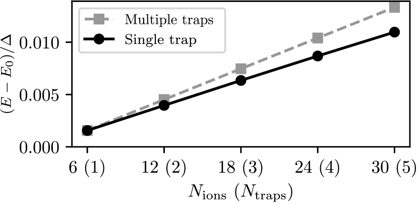
In Fig. 6, we compare the excitation energies, from optimizing the QDB-MPS circuit, with a single trap and with a modular trap network. Both circuits have the same number of variational operations in the boxes in the edges and in the boxes of the bulk, and the interface operation contains variational sideband operations. The error emerging from the optimization of the ion-trap network deviates only slightly from the error in the single trap case, and we recover linear scaling of the error with the system size. This result is an even stronger indicator of scalability of the QDB-MPS approach for VQE, as it can treat hardware interfaces as impurities, and efficiently compensate for them with small variations of the circuit ansatz.
5 Outlook
We proposed an approach for VQE which uses qubit-QDB interactions, available in currently-existing programmable quantum devices, as variational resource operations. In our strategy, the QDB is disentangled from the optimized states only at the end of the state preparation, as a byproduct of the optimization. For trapped ions, we discussed how to realize our strategy with resonant blue-sideband pulses, potentially yielding faster state-preparation rates compared to existing strategies, and thus helping to mitigate decoherence effects. The variational ansatz circuit we designed is tailored to efficiently prepare MPS, leading to a potential improvement in scalability over current VQE strategies.
We numerically simulated the ion trap implementation of VQE based on the QDB-MPS ansatz circuit, and showed strong evidence of scalability of our approach, even when it is realized in modular ion traps. While the ions-COM mode sideband interactions operate in an extended Hilbert space, we demonstrated that these resource operations can incorporate symmetries in the variational circuit, similar to the closed-system VQE approaches. Although here we demonstrated robustness of the method to the initial temperature of the COM mode, further investigations are required to study other realistic imperfections, including (i) qubits decoherence, (ii) fluctuations of the control parameters, and (iii) shot noise resulting from a finite budget of measurements to reconstruct the cost function.
The developed QDB-based VQE can be readily used in other currently available experimental platforms, such as quantum dots [71] or atoms coupled by (chiral) waveguides [72]. Moreover, we expect that the scaling and parametric efficiency of our results, found for the MPS circuit ansatz, extend to other efficiently-contractible tensor network states [58, 61], such as [73, 74], thus allowing us to accomodate the entanglement content required to explore higher dimensions. Also, by including simultaneous operations on multiple qubits, it is possible to build many-body wavefunction ansätze beyond tensor networks, ultimately enabling the efficient preparation of quantum states that can not be numerically simulated. Finally, we envision the possibility of including controllable dissipative elements to the QDB resources [75] in order to construct optimized cooling algorithms beyond stabilizer codes [76, 77].
Appendix
Appendix A Maximum bond dimension
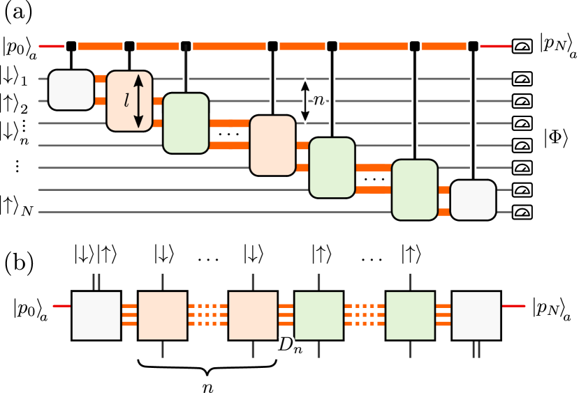
In the section, we study the maximum bond dimension, , of MPS generated with the QDB-MPS circuit using a bosonic QDB and built with resource operations (1) described by the Anti-Jaynes-Cummings Hamiltonian. Here we distinguish two sets of MPS accessible by the circuit. The first set contains all pure states which can be generated by the QDB-MPS circuit. The states of this set can be generated probabilistically [59] after measuring (and therefore disentangling) the QDB at the end. It defines the search space for VQE and, therefore, is desired to be limited. The second set — a subset of the first set — contains deterministically generated translationally invariant MPS, which are disentangled from the QDB by the end of the circuit without measuring the EM. This set, in opposite to the first one, is required to be big enough to include a good approximation of the target state.
Set of probabilistically generated MPS
We start with the set of MPS generated probabilistically. We characterize this set of MPS by considering a possible range of their bond dimensions. Bond dimension of MPS of size is the maximum of bond dimensions between two blocks of qubits and . corresponds to entanglement entropy between the blocks [57], such that the Schmidt decomposition of MPS in the basis of two blocks and is
The entanglement entropy of the blocks is , with the state of qubits .
Using singular value decomposition, one can show that, for an arbitrary state of size , it is valid that , and, therefore, . By using a not universal set of resource operations (9) we limit and, therefore, restrict the set of achievable states. As presented in Appendix B, interactions (1) preserve an extended symmetry . In the following, we explain that this symmetry imposes , where is the size of the bulk boxes in the QDB-MPS circuit, and limits the maximum bond dimension as . Therefore, in comparison with the general case, the bond dimension of the MPS generated by the QDB-MPS circuit is exponentially suppressed.
Figure 7, demonstrates entanglement distribution in the QDB-MPS circuit between the qubits by a subsystem, highlighted by orange color, which includes the QDB and qubits shared by neighbor virtual boxes. Such a subsystem can be considered as a virtual ancilla that sequentially interacts with the qubits distributing entanglement among them [59]. The effective dimension of this ancilla (dimension of the populated Hilbert space) bounds bond dimension .
Let us consider the QDB initially prepared in state , and the qubits prepared in state . Then, because of the preserved symmetry, the maximum possible population of the QDB after interaction with ions can not be higher than . Multiplying the growing dimension of the QDB by the dimension of qubits in the ancilla, we obtain that . From the other side, as explained in [59], has to decrease as approaches to to guarantee that the ancilla (with QDB measured in ) is decoupled by the end of the state preparation. Therefore, there exists some , for which achieves its maximum. To obtain , we study how can decrease while the ancilla interacts with the qubits after qubit . Intuitively, this can be done other way around by considering the growth of bond dimension if MPS would be generated from the other side of the qubits chain, starting from . Since the measured output state can contain number of excitations , the number of excitations in the QDB can not only increase but also decrease as the QDB interacts with the qubits, populating Hilbert space with the twice bigger dimension than if the QDB would be initially prepared in . Therefore, . Solving we obtain that, after , has to decrease with . Thus, we find that .
Set of deterministically generated translationally invariant MPS
In order to generate MPS with translationally invariant in the bulk, the virtual ancilla has to own dimension which repeats itself with a target period along the state preparation. This includes the ancilla dimension after realization of the last box in the bulk, after which the edge box is aimed to disentangle the QDB from ancilla qubits as required by deterministic preparation of a pure state. This can be done only if the effective dimension of the ancilla does not exceed dimension of the qubits. Hence, the limit of the bond dimension of the translationally invariant MPS deterministically generated in the considered QDB-MPS circuit is . Here, we defined the limit not exactly, since the actual bond dimension can vary within one period of the bulk.
Appendix B Symmetries
In this section, we discuss the symmetries protected by the operations
| (9) |
with the Rabi frequency, is the destruction operator for the bosonic QDB, and the lowering operator for qubit , with the internal logical states of the qubit.
Magnetization A number symmetry, forming an Abelian group of symmetric transformations , is generated by the integer operator
| (10) |
where is the number of qubits, , and . It is straightforward to check that is a symmetry since for every site . thus defines a quantum number, which is conserved during the controlled variational dynamics. Consider the initial state of the system of qubits plus the QDB as , with the state of the qubits and the Fock state of the QDB, , . This state has well-defined quantum number . Due to the symmetry of Eq. (10), the evolution of this state will preserve its quantum number, and the state will always be of the form , where the qubit states are labeled by the magnetization (eigenvalues of ) and degeneracy . At the end of the variational quantum state preparation, after optimization of the process, the output state will be disentangled between phonon and qubits, and reads . The final qubit state will thus have a well-defined magnetization . This requirement identifies the class of target Hamiltonians targetable with the chosen resources: which must contain the magnetization symmetry: .
Conjugation A second symmetry is nested within our controls, and it becomes evident after gauging the resource Hamiltonians as in Eq. (1). In this format, the resource Hamiltonians are purely imaginary when expressed in the canonical basis, and thus antisymmetric and traceless . It follows that the unitary operators of time evolution under must be real, as they are imaginary exponentials of imaginary matrices, and have determinant . This means that, with the chosen resources, we can only perform transformations in the special orthogonal group SO(), a subgroup of the unitaries U(), which, in turn, limits the set of states we can prepare to real states (vectors with real coefficients in the canonical basis). In conclusion, the class of models targetable with our variational scheme is restricted to models expressed by real, or symmetric, Hamiltonians, which always possess real eigenbases. We stress that the complex conjugation symmetry can be relaxed by adding a detuning to one or more of the control lasers, which can be helpful if we aim to quantum simulate a non-real Hamiltonian .
Appendix C Controllability
We now discuss the controllability problem and show that, within the constraints set in the symmetry section, the selected controls are theoretically able to prepare any quantum state, in the limit of infinite available resources. First of all, we argue that starting from the state it is possible to shift the system qubits state to any magnetization sector. This is shown recursively, by highlighting that the state under the action of for a time equal to is completely mapped into the state , ultimately increasing the magnetization by +1. Secondly, we show that our controls provide strong controllability within each magnetization sector (of dimension ) of real states, meaning that the Lie algebra generated by contains the Lie algebra of imaginary, hermitian matrices onto the sector, generators of SO, as we will show later in this section. From this observation, it follows that any two real states and can be dynamically connected, i.e., for some , simply because the effective Hamiltonian , with , can be generated with our resources.
We now prove that, by means of linear combination and commutation, we can generate the whole algebra of imaginary Hermitian matrices for the sector by starting from the bare resources . We start by considering the commutator , for sites , which is an endomorphism of magnetization sector . Moreover, it is easy to show that , for . By recursion and locality, it follows that we can generate any string operator of the form
| (11) |
for any binary string . We run one additional commutator, namely where all sites are different. By recursion, we conclude that we can generate operators which are tensor product of one operator at a pair of sites , any amount of , and any amount of (each one acting on separate sites). We remark that these operators form a basis for the imaginary Hermitian endomorphisms of the symmetry sector . To see this, consider the canonical basis , where and are any two-bit strings with total magnetization . This operator can be easily decomposed in operators of the form : for bits that do not flip () just insert a in the tensor product string, while for pairs of bits that flip-flop, insert a , except one, which is substituted by . This concludes the proof.
Appendix D Parameters optimization
In the section, we describe the method used for the optimization of variational parameters in the numerical simulations of VQE with the circuits given in the main text. Since the purpose of the paper is to study the achievable accuracy of the proposed approaches, we employ the exact value of cost function in the optimization. The expectation value is obtained by simulating the circuits in terms of density matrixes without considering shot noise caused by the finite number of measurements of the trial ions states. To optimize parameters we use a gradient-based optimization algorithm, which relies on numerically accessible approximate values of . To be more precise, we use the basin-hopping method [78, 79], which is a two-phase method that combines a global stepping algorithm with local minimization at each step. As a local minimization algorithm, we use the quasi-newton method of Broyden, Fletcher, Goldfarb, and Shanno (BFGS) [80, 81, 82, 83].
To decrease noise in the data presented in the result section, we ensured that is monotonically decreases with decrease of temperature of the COM mode (or equivalently number of excitations ), with decrease of state size , and with growth of the number of variational parameters . We begin by independently optimizing parameters for all data points (defined by one or two values of , , and ), each of which starts from several sets of initial parameters with values . Then, the optimized parameters of the best result in one data point is used as the initial parameters set for the neighbor data point, and the obtained result is compared with the existing ones. In the case when the neighbor data point requires less initial parameters, the extra parameters are removed from the inserted parameters set; otherwise, parameters with can be inserted. To obtain the presented data, we iteratively re-optimize the parameters from one side of data points range to another and, afterward, in the reverse direction until convergence.
Appendix E Gates sequence in the circuit
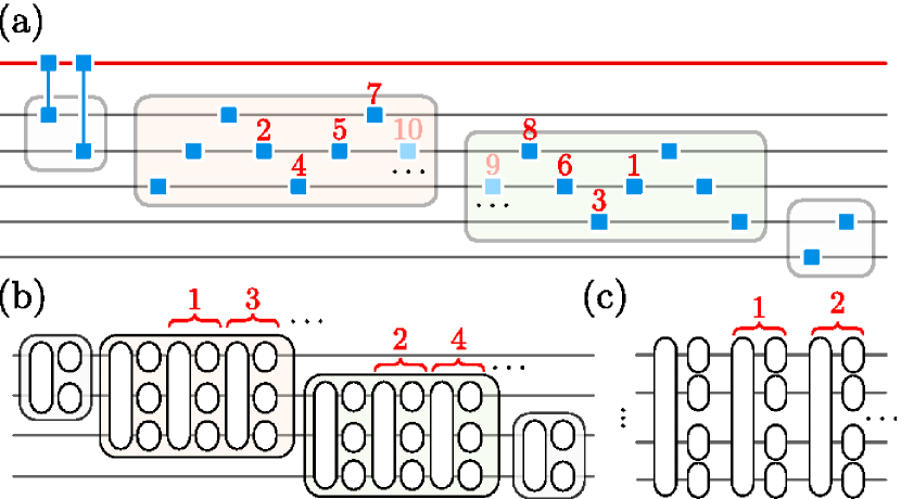
In the section, we consider in detail the sequences of variational operations, Fig. (8), used to construct circuits considered in our work. The number of variational operations in the edge boxes of the QDB-MPS and CSD-MPS circuits is fixed to and 3 correspondingly, as shown in Fig. (8). In these circuits, the number of variational parameters is increased by progressively inserting operations in the first bulk box (orange) or second (green), alternately. In the QDB-MPS circuit, we increase this number by 1, arranging the operations such that the last operation in one box and the first in the next box do not act to the same qubit. In the CSD-MPS circuit, we add a single layer, consisting of a local MS operation and rotations at each ion. To increase the number of variational operations in the CSA circuit, we add a single layer consisting of operations and per ion.
The trial states in the CSA circuit are obtained as , with the resource operations. Afterward, the required correlation functions can be obtained from . Since this method requires numerical operation with the full quantum state, the number of the qubits in the CSA circuit in our study is limited by . On the contrary, one can see from Fig. 8 that, in order to obtain correlation functions of the states generated by the QDB-MPS and CSD-MPS, the full state is not required to be kept, but only a reduced density matrix of at maximum qubits plus the QDB, with the size of the bulk boxes. The qubits which do not more participate in the evolution until the end of the circuit can be measured in the required bases, and the next qubit can be added to the remained qubits state by using the Kronecker product operation.
Appendix F Energy bounds on fidelity and purity
In this section, we show that the final energy , in respect to a target Hamiltonian , measured on the optimized variational quantum state imposes a bound on its fidelity , with the exact ground state. Establishing this bound requires a good estimate of the two lowest energy levels and , which can be estimated on the quantum device via a subspace expansion technique for mixed states, illustrated in detail in the Supplementary Information of Ref. [84]. This analysis provides self-verification of the variational quantum state preparation algorithm [23]. Alternatively, for 1D lattice Hamiltonians, and can be obtained using numerical method DMRG.
Let us consider the following inequality
| (12) |
stating that the state fidelity is bound from below by the ratio
| (13) |
delivering an actual (positive) bound only when the variational state energy is below the first excited energy, i.e. . A lower bound on the fidelity, in turn, infers a bound on the purity . In fact
| (14) |
In conclusion, as long as , we have that
| (15) |
approaching (certified pure state) in the limit .
References
- Endres et al. [2016] M. Endres, H. Bernien, A. Keesling, H. Levine, E. R. Anschuetz, A. Krajenbrink, C. Senko, V. Vuletic, M. Greiner, and M. D. Lukin. Atom-by-atom assembly of defect-free one-dimensional cold atom arrays. Science, 354, 1024–1027, (2016). http://dx.doi.org/10.1126/science.aah3752.
- Gross and Bloch [2017] C. Gross and I. Bloch. Quantum simulations with ultracold atoms in optical lattices. Science, 357, 995–1001, (2017). http://dx.doi.org/10.1126/science.aal3837.
- King et al. [2018] A. D. King, J. Carrasquilla, J. Raymond, I. Ozfidan, E. Andriyash, A. Berkley, M. Reis, T. Lanting, R. Harris, F. Altomare, K. Boothby, P. I. Bunyk, C. Enderud, A. Fréchette, E. Hoskinson, N. Ladizinsky, T. Oh, G. Poulin-Lamarre, C. Rich, Y. Sato, A. Y. Smirnov, L. J. Swenson, M. H. Volkmann, J. Whittaker, J. Yao, E. Ladizinsky, M. W. Johnson, J. Hilton, and M. H. Amin. Observation of topological phenomena in a programmable lattice of 1,800 qubits. Nature, 560, 456–460, (2018). http://dx.doi.org/10.1038/s41586-018-0410-x.
- Hebenstreit et al. [2013] F. Hebenstreit, J. Berges, and D. Gelfand. Real-time dynamics of string breaking. Physical Review Letters, 111, 1–5, (2013). http://dx.doi.org/10.1103/PhysRevLett.111.201601.
- Jurcevic et al. [2014] P. Jurcevic, B. P. Lanyon, P. Hauke, C. Hempel, P. Zoller, R. Blatt, and C. F. Roos. Quasiparticle engineering and entanglement propagation in a quantum many-body system. Nature, 511, 202–205, (2014). http://dx.doi.org/10.1038/nature13461.
- Martinez et al. [2016] E. A. Martinez, C. A. Muschik, P. Schindler, D. Nigg, A. Erhard, M. Heyl, P. Hauke, M. Dalmonte, T. Monz, P. Zoller, and R. Blatt. Real-time dynamics of lattice gauge theories with a few-qubit quantum computer. Nature, 534, 516–519, (2016). http://dx.doi.org/10.1038/nature18318.
- Pichler et al. [2016a] T. Pichler, M. Dalmonte, E. Rico, P. Zoller, and S. Montangero. Real-time dynamics in U(1) lattice gauge theories with tensor networks. Physical Review X, 6, 1–17, (2016). http://dx.doi.org/10.1103/PhysRevX.6.011023.
- Kitagawa and Ueda [1993] M. Kitagawa and M. Ueda. Squeezed spin states. Phys. Rev. A, 47, 5138–5143, (1993). http://dx.doi.org/10.1103/PhysRevA.47.5138.
- Pichler et al. [2016b] T. Pichler, T. Caneva, S. Montangero, M. D. Lukin, and T. Calarco. Noise-resistant optimal spin squeezing via quantum control. Phys. Rev. A, 93, 013851, (2016). http://dx.doi.org/10.1103/PhysRevA.93.013851.
- Kaubruegger et al. [2019] R. Kaubruegger, P. Silvi, C. Kokail, R. van Bijnen, A. M. Rey, J. Ye, A. M. Kaufman, and P. Zoller. Variational Spin-Squeezing Algorithms on Programmable Quantum Sensors. Phys. Rev. Lett., 123, 260505, (2019). http://dx.doi.org/10.1103/PhysRevLett.123.260505.
- Volkoff [2016] T. Volkoff. Optimal and near-optimal probe states for quantum metrology of number-conserving two-mode bosonic Hamiltonians. Physical Review A, 94, 042327, (2016).
- Richerme et al. [2013a] P. Richerme, C. Senko, J. Smith, A. Lee, S. Korenblit, and C. Monroe. Experimental performance of a quantum simulator: Optimizing adiabatic evolution and identifying many-body ground states. Phys. Rev. A, 88, 012334, (2013). http://dx.doi.org/10.1103/PhysRevA.88.012334.
- Bernien et al. [2017] H. Bernien, S. Schwartz, A. Keesling, H. Levine, A. Omran, H. Pichler, S. Choi, A. S. Zibrov, M. Endres, M. Greiner, V. Vuletic, and M. D. Lukin. Probing many-body dynamics on a 51-atom quantum simulator. Nature, 551, 579–584, (2017). http://dx.doi.org/10.1038/nature24622.
- Richerme et al. [2013b] P. Richerme, C. Senko, J. Smith, A. Lee, S. Korenblit, and C. Monroe. Experimental performance of a quantum simulator: Optimizing adiabatic evolution and identifying many-body ground states. Phys. Rev. A, 88, 012334, (2013). http://dx.doi.org/10.1103/PhysRevA.88.012334.
- Peruzzo et al. [2014] A. Peruzzo, J. McClean, P. Shadbolt, M.-H. Yung, X.-Q. Zhou, P. J. Love, A. Aspuru-Guzik, and J. L. O’Brien. A variational eigenvalue solver on a photonic quantum processor. Nature communications, 5, 4213, (2014). http://dx.doi.org/10.1038/ncomms5213.
- Farhi et al. [2014] E. Farhi, J. Goldstone, and S. Gutmann. A quantum approximate optimization algorithm. MIT-CTP/4610, (2014).
- McClean et al. [2016] J. R. McClean, J. Romero, R. Babbush, and A. Aspuru-Guzik. The theory of variational hybrid quantum-classical algorithms. New Journal of Physics, 18, 023023, (2016). http://dx.doi.org/10.1088/1367-2630/18/2/023023.
- Kandala et al. [2017] A. Kandala, A. Mezzacapo, K. Temme, M. Takita, M. Brink, J. M. Chow, and J. M. Gambetta. Hardware-efficient variational quantum eigensolver for small molecules and quantum magnets. Nature, 549, 242, (2017). http://dx.doi.org/10.1038/nature23879.
- Yang et al. [2017] Z.-C. Yang, A. Rahmani, A. Shabani, H. Neven, and C. Chamon. Optimizing Variational Quantum Algorithms Using Pontryagin’s Minimum Principle. Phys. Rev. X, 7, 021027, (2017). http://dx.doi.org/10.1103/PhysRevX.7.021027.
- Doria et al. [2011] P. Doria, T. Calarco, and S. Montangero. Optimal Control Technique for Many-Body Quantum Dynamics. Phys. Rev. Lett., 106, 190501, (2011). http://dx.doi.org/10.1103/PhysRevLett.106.190501.
- Klco et al. [2018] N. Klco, E. F. Dumitrescu, A. J. McCaskey, T. D. Morris, R. C. Pooser, M. Sanz, E. Solano, P. Lougovski, and M. J. Savage. Quantum-classical computation of Schwinger model dynamics using quantum computers. Phys. Rev. A, 98, 032331, (2018). http://dx.doi.org/10.1103/PhysRevA.98.032331.
- Hempel et al. [2018] C. Hempel, C. Maier, J. Romero, J. McClean, T. Monz, H. Shen, P. Jurcevic, B. P. Lanyon, P. Love, R. Babbush, A. Aspuru-Guzik, R. Blatt, and C. F. Roos. Quantum Chemistry Calculations on a Trapped-Ion Quantum Simulator. Phys. Rev. X, 8, 031022, (2018). http://dx.doi.org/10.1103/PhysRevX.8.031022.
- Kokail et al. [2019] C. Kokail, C. Maier, R. van Bijnen, T. Brydges, M. K. Joshi, P. Jurcevic, C. A. Muschik, P. Silvi, R. Blatt, C. F. Roos, and P. Zoller. Self-verifying variational quantum simulation of lattice models. Nature, 569, 355–360, (2019). http://dx.doi.org/10.1038/s41586-019-1177-4.
- Smith et al. [2016] J. Smith, A. Lee, P. Richerme, B. Neyenhuis, P. W. Hess, P. Hauke, M. Heyl, D. A. Huse, and C. Monroe. Many-body localization in a quantum simulator with programmable random disorder. Nature Physics, 12, 907–911, (2016). http://dx.doi.org/10.1038/nphys3783.
- Elben et al. [2020] A. Elben, B. Vermersch, R. van Bijnen, C. Kokail, T. Brydges, C. Maier, M. K. Joshi, R. Blatt, C. F. Roos, and P. Zoller. Cross-Platform Verification of Intermediate Scale Quantum Devices. Phys. Rev. Lett., 124, 010504, (2020). http://dx.doi.org/10.1103/PhysRevLett.124.010504.
- Cirac and Zoller [1995] J. I. Cirac and P. Zoller. Quantum Computations with Cold Trapped Ions. Physical Review Letters, 74, 4091–4094, (1995). http://dx.doi.org/10.1103/PhysRevLett.74.4091.
- Su et al. [1979] W. P. Su, J. R. Schrieffer, and A. J. Heeger. Solitons in Polyacetylene. Phys. Rev. Lett., 42, 1698–1701, (1979). http://dx.doi.org/10.1103/PhysRevLett.42.1698.
- Su et al. [1980] W. P. Su, J. R. Schrieffer, and A. J. Heeger. Soliton excitations in polyacetylene. Phys. Rev. B, 22, 2099–2111, (1980). http://dx.doi.org/10.1103/PhysRevB.22.2099.
- Asbóth et al. [2016] J. K. Asbóth, L. Oroszlány, and A. Pályi. The Su-Schrieffer-Heeger (SSH) Model, pages 1–22. Springer, (2016). http://dx.doi.org/10.1007/978-3-319-25607-8_1.
- Gardiner and Zoller [2015] C. Gardiner and P. Zoller. The quantum world of ultra-cold atoms and light book II: the physics of quantum-optical devices. World Scientific Publishing Company, (2015). http://dx.doi.org/10.1142/p983.
- Östlund and Rommer [1995] S. Östlund and S. Rommer. Thermodynamic Limit of Density Matrix Renormalization. Phys. Rev. Lett., 75, 3537–3540, (1995). http://dx.doi.org/10.1103/PhysRevLett.75.3537.
- Verstraete et al. [2004] F. Verstraete, D. Porras, and J. I. Cirac. Density Matrix Renormalization Group and Periodic Boundary Conditions: A Quantum Information Perspective. Phys. Rev. Lett., 93, 227205, (2004). http://dx.doi.org/10.1103/PhysRevLett.93.227205.
- Blatt and Wineland [2008] R. Blatt and D. Wineland. Entangled states of trapped atomic ions. Nature, 453, 1008–1015, (2008). http://dx.doi.org/10.1038/nature07125.
- Monroe and Kim [2013] C. Monroe and J. Kim. Scaling the Ion Trap Quantum Processor. Science, 339, 1164–1169, (2013). http://dx.doi.org/10.1126/science.1231298.
- Hood et al. [2016] J. D. Hood, A. Goban, A. Asenjo-Garcia, M. Lu, S. P. Yu, D. E. Chang, and H. J. Kimble. Atom-atom interactions around the band edge of a photonic crystal waveguide. Proceedings of the National Academy of Sciences of the United States of America, 113, 10507–10512, (2016). http://dx.doi.org/10.1073/pnas.1603788113.
- Yu et al. [2019] S. P. Yu, J. A. Muniz, C. L. Hung, and H. J. Kimble. Two-dimensional photonic crystals for engineering atom–light interactions. Proceedings of the National Academy of Sciences of the United States of America, 116, 12743–12751, (2019). http://dx.doi.org/10.1073/pnas.1822110116.
- Kollár et al. [2017] A. J. Kollár, A. T. Papageorge, V. D. Vaidya, Y. Guo, J. Keeling, and B. L. Lev. Supermode-density-wave-polariton condensation with a Bose-Einstein condensate in a multimode cavity. Nature Communications, 8, 1–10, (2017). http://dx.doi.org/10.1038/ncomms14386.
- Cohen and Mølmer [2018] I. Cohen and K. Mølmer. Deterministic quantum network for distributed entanglement and quantum computation. Phys. Rev. A, 98, 030302, (2018). http://dx.doi.org/10.1103/PhysRevA.98.030302.
- Vaidya et al. [2018] V. D. Vaidya, Y. Guo, R. M. Kroeze, K. E. Ballantine, A. J. Kollár, J. Keeling, and B. L. Lev. Tunable-Range, Photon-Mediated Atomic Interactions in Multimode Cavity QED. Physical Review X, 8, 11002, (2018). http://dx.doi.org/10.1103/PhysRevX.8.011002.
- Welte et al. [2018] S. Welte, B. Hacker, S. Daiss, S. Ritter, and G. Rempe. Photon-Mediated Quantum Gate between Two Neutral Atoms in an Optical Cavity. Phys. Rev. X, 8, 011018, (2018). http://dx.doi.org/10.1103/PhysRevX.8.011018.
- Fitzpatrick et al. [2017] M. Fitzpatrick, N. M. Sundaresan, A. C. Li, J. Koch, and A. A. Houck. Observation of a dissipative phase transition in a one-dimensional circuit QED lattice. Physical Review X, 7, 1–8, (2017). http://dx.doi.org/10.1103/PhysRevX.7.011016.
- Fink et al. [2017] J. M. Fink, A. Dombi, A. Vukics, A. Wallraff, and P. Domokos. Observation of the photon-blockade breakdown phase transition. Physical Review X, 7, 1–9, (2017). http://dx.doi.org/10.1103/PhysRevX.7.011012.
- Song et al. [2017] C. Song, K. Xu, W. Liu, C.-p. Yang, S.-B. Zheng, H. Deng, Q. Xie, K. Huang, Q. Guo, L. Zhang, P. Zhang, D. Xu, D. Zheng, X. Zhu, H. Wang, Y.-A. Chen, C.-Y. Lu, S. Han, and J.-W. Pan. 10-Qubit Entanglement and Parallel Logic Operations with a Superconducting Circuit. Physical Review Letters, 119, 180511, (2017). http://dx.doi.org/10.1103/PhysRevLett.119.180511.
- Schuetz et al. [2019] M. J. A. Schuetz, B. Vermersch, G. Kirchmair, L. M. K. Vandersypen, J. I. Cirac, M. D. Lukin, and P. Zoller. Quantum simulation and optimization in hot quantum networks. Phys. Rev. B, 99, 241302, (2019). http://dx.doi.org/10.1103/PhysRevB.99.241302.
- Shi et al. [2015] T. Shi, D. E. Chang, and J. I. Cirac. Multiphoton-scattering theory and generalized master equations. Physical Review A, 92, 053834, (2015). http://dx.doi.org/10.1103/PhysRevA.92.053834.
- Sillanpää et al. [2007] M. A. Sillanpää, J. I. Park, and R. W. Simmonds. Coherent quantum state storage and transfer between two phase qubits via a resonant cavity. Nature, 449, 438–442, (2007). http://dx.doi.org/10.1038/nature06124.
- Lemmer et al. [2013] A. Lemmer, A. Bermudez, and M. B. Plenio. Driven geometric phase gates with trapped ions. New Journal of Physics, 15, 083001, (2013). http://dx.doi.org/10.1088/1367-2630/15/8/083001.
- Debnath et al. [2018] S. Debnath, N. M. Linke, S. T. Wang, C. Figgatt, K. A. Landsman, L. M. Duan, and C. Monroe. Observation of Hopping and Blockade of Bosons in a Trapped Ion Spin Chain. Physical Review Letters, 120, 73001, (2018). http://dx.doi.org/10.1103/PhysRevLett.120.073001.
- Mølmer and Sørensen [1999] K. Mølmer and A. Sørensen. Multiparticle Entanglement of Hot Trapped Ions. Physical Review Letters, 82, 1835–1838, (1999). http://dx.doi.org/10.1103/PhysRevLett.82.1835.
- Porras and Cirac [2004] D. Porras and J. I. Cirac. Effective Quantum Spin Systems with Trapped Ions. Phys. Rev. Lett., 92, 207901, (2004). http://dx.doi.org/10.1103/PhysRevLett.92.207901.
- Majer et al. [2007] J. Majer, J. M. Chow, J. M. Gambetta, J. Koch, B. R. Johnson, J. A. Schreier, L. Frunzio, D. I. Schuster, A. A. Houck, A. Wallraff, A. Blais, M. H. Devoret, S. M. Girvin, and R. J. Schoelkopf. Coupling superconducting qubits via a cavity bus. Nature, 449, 443–447, (2007). http://dx.doi.org/10.1038/nature06184.
- Douglas et al. [2015] J. S. Douglas, H. Habibian, C. L. Hung, A. V. Gorshkov, H. J. Kimble, and D. E. Chang. Quantum many-body models with cold atoms coupled to photonic crystals. Nature Photonics, 9, 326–331, (2015). http://dx.doi.org/10.1038/nphoton.2015.57.
- Sackett et al. [2000] C. A. Sackett, D. Kielpinski, B. E. King, C. Langer, V. Meyer, C. J. Myatt, M. Rowe, Q. A. Turchette, W. M. Itano, D. J. Wineland, and C. Monroe. Experimental entanglement of four particles. Nature, 404, 256–259, (2000). http://dx.doi.org/10.1038/35005011.
- Friis et al. [2018] N. Friis, O. Marty, C. Maier, C. Hempel, M. Holzäpfel, P. Jurcevic, M. B. Plenio, M. Huber, C. Roos, R. Blatt, and B. Lanyon. Observation of Entangled States of a Fully Controlled 20-Qubit System. Phys. Rev. X, 8, 021012, (2018). http://dx.doi.org/10.1103/PhysRevX.8.021012.
- Georgescu et al. [2014] I. M. Georgescu, S. Ashhab, and F. Nori. Quantum simulation. Reviews of Modern Physics, 86, 153–185, (2014). http://dx.doi.org/10.1103/RevModPhys.86.153.
- Schollwöck [2011] U. Schollwöck. The density-matrix renormalization group in the age of matrix product states. Annals of Physics, 326, 96–192, (2011). http://dx.doi.org/10.1016/j.aop.2010.09.012.
- Orús [2014] R. Orús. A practical introduction to tensor networks: Matrix product states and projected entangled pair states. Annals of Physics, 349, 117–158, (2014). http://dx.doi.org/10.1016/j.aop.2014.06.013.
- Huggins et al. [2018] W. Huggins, P. Patel, K. B. Whaley, and E. M. Stoudenmire. Towards Quantum Machine Learning with Tensor Networks. Quantum Science and Technology, 4, 024001, (2018). http://dx.doi.org/10.1088/2058-9565/aaea94.
- Schön et al. [2007] C. Schön, K. Hammerer, M. M. Wolf, J. I. Cirac, and E. Solano. Sequential generation of matrix-product states in cavity QED. Phys. Rev. A, 75, 032311, (2007). http://dx.doi.org/10.1103/PhysRevA.75.032311.
- Ran [2019] S.-J. Ran. Efficient Encoding of Matrix Product States into Quantum Circuits of One-and Two-Qubit Gates. arXiv preprint arXiv:1908.07958, (2019).
- Liu et al. [2019] J.-G. Liu, Y.-H. Zhang, Y. Wan, and L. Wang. Variational quantum eigensolver with fewer qubits. Phys. Rev. Research, 1, 023025, (2019). http://dx.doi.org/10.1103/PhysRevResearch.1.023025.
- Roos et al. [1999] C. Roos, T. Zeiger, H. Rohde, H. C. Nägerl, J. Eschner, D. Leibfried, F. Schmidt-Kaler, and R. Blatt. Quantum State Engineering on an Optical Transition and Decoherence in a Paul Trap. Phys. Rev. Lett., 83, 4713–4716, (1999). http://dx.doi.org/10.1103/PhysRevLett.83.4713.
- Schäfer et al. [2018] V. M. Schäfer, C. J. Ballance, K. Thirumalai, L. J. Stephenson, T. G. Ballance, A. M. Steane, and D. M. Lucas. Fast quantum logic gates with trapped-ion qubits. Nature, 555, 75–78, (2018). http://dx.doi.org/10.1038/nature25737.
- Borkar et al. [2015] V. S. Borkar, V. R. Dwaracherla, and N. Sahasrabudhe. Gradient Estimation with Simultaneous Perturbation and Compressive Sensing. Journal of Machine Learning Research, 18, 1–27, (2015).
- Prashanth et al. [2016] L. Prashanth, S. Bhatnagar, M. Fu, and S. Marcus. Adaptive system optimization using random directions stochastic approximation. IEEE Transactions on Automatic Control, 62, 2223–2238, (2016). http://dx.doi.org/10.1109/TAC.2016.2600643.
- Leng et al. [2019] Z. Leng, P. Mundada, S. Ghadimi, and A. Houck. Robust and efficient algorithms for high-dimensional black-box quantum optimization. arXiv preprint arXiv:1910.03591, (2019).
- Nicholas [2014] P. Nicholas. A dividing rectangles algorithm for stochastic simulation optimization. In Proc. INFORMS Comput. Soc. Conf., volume 14, pages 47–61, (2014). http://dx.doi.org/10.1287/ics.2015.0004.
- Liu et al. [2015] H. Liu, S. Xu, X. Wang, J. Wu, and Y. Song. A global optimization algorithm for simulation-based problems via the extended DIRECT scheme. Engineering Optimization, 47, 1441–1458, (2015). http://dx.doi.org/10.1080/0305215X.2014.971777.
- White [1992] S. R. White. Density matrix formulation for quantum renormalization groups. Phys. Rev. Lett., 69, 2863–2866, (1992). http://dx.doi.org/10.1103/PhysRevLett.69.2863.
- Bowler et al. [2012] R. Bowler, J. Gaebler, Y. Lin, T. R. Tan, D. Hanneke, J. D. Jost, J. P. Home, D. Leibfried, and D. J. Wineland. Coherent Diabatic Ion Transport and Separation in a Multi-Zone Trap Array. Physical Review Letters, 109, 1–4, (2012). http://dx.doi.org/10.1103/PhysRevLett.109.080502.
- Baart et al. [2017] T. A. Baart, T. Fujita, C. Reichl, W. Wegscheider, and L. M. K. Vandersypen. Coherent spin-exchange via a quantum mediator. Nature Nanotechnology, 12, 26–30, (2017). http://dx.doi.org/10.1038/nnano.2016.188.
- Lodahl et al. [2016] P. Lodahl, S. Mahmoodian, S. Stobbe, P. Schneeweiss, J. Volz, A. Rauschenbeutel, H. Pichler, and P. Zoller. Chiral Quantum Optics. Nature, 541, 473–480, (2016). http://dx.doi.org/10.1038/nature21037.
- Zaletel and Pollmann [2019] M. P. Zaletel and F. Pollmann. Isometric Tensor Network States in Two Dimensions. arXiv preprint arXiv:1902.05100, (2019).
- Haghshenas et al. [2019] R. Haghshenas, M. J. O’Rourke, and G. K.-L. Chan. Conversion of projected entangled pair states into a canonical form. Phys. Rev. B, 100, 054404, (2019). http://dx.doi.org/10.1103/PhysRevB.100.054404.
- Rivas and Huelga [2012] A. Rivas and S. F. Huelga. Open quantum systems. Springer, (2012). http://dx.doi.org/10.1007/978-3-642-23354-8.
- Shor [1995] P. W. Shor. Scheme for reducing decoherence in quantum computer memory. Phys. Rev. A, 52, R2493–R2496, (1995). http://dx.doi.org/10.1103/PhysRevA.52.R2493.
- Reiter et al. [2017] F. Reiter, A. S. Sørensen, P. Zoller, and C. A. Muschik. Dissipative quantum error correction and application to quantum sensing with trapped ions. Nature Communications, 8, 1822, (2017). http://dx.doi.org/10.1038/s41467-017-01895-5.
- Wales and Doye [1997] D. J. Wales and J. P. Doye. Global optimization by basin-hopping and the lowest energy structures of Lennard-Jones clusters containing up to 110 atoms. The Journal of Physical Chemistry A, 101, 5111–5116, (1997). http://dx.doi.org/10.1021/jp970984n.
- Olson et al. [2012] B. Olson, I. Hashmi, K. Molloy, and A. Shehu. Basin hopping as a general and versatile optimization framework for the characterization of biological macromolecules. Advances in Artificial Intelligence, 2012, 3, (2012). http://dx.doi.org/10.1155/2012/674832.
- Broyden [1970] C. G. Broyden. The convergence of a class of double-rank minimization algorithms 1. general considerations. IMA Journal of Applied Mathematics, 6, 76–90, (1970). http://dx.doi.org/doi.org/10.1093/imamat/6.1.76.
- Fletcher [1970] R. Fletcher. A new approach to variable metric algorithms. The computer journal, 13, 317–322, (1970). http://dx.doi.org/10.1093/comjnl/13.3.317.
- Goldfarb [1970] D. Goldfarb. A family of variable-metric methods derived by variational means. Mathematics of computation, 24, 23–26, (1970). http://dx.doi.org/10.1090/S0025-5718-1970-0258249-6.
- Shanno [1970] D. F. Shanno. Conditioning of quasi-Newton methods for function minimization. Mathematics of computation, 24, 647–656, (1970). http://dx.doi.org/10.1090/S0025-5718-1970-0274029-X.
- Colless et al. [2018] J. I. Colless, V. V. Ramasesh, D. Dahlen, M. S. Blok, M. E. Kimchi-Schwartz, J. R. McClean, J. Carter, W. A. De Jong, and I. Siddiqi. Computation of Molecular Spectra on a Quantum Processor with an Error-Resilient Algorithm. Physical Review X, 8, 11021, (2018). http://dx.doi.org/10.1103/PhysRevX.8.011021.
