Adjoint computations by algorithmic differentiation of a parallel solver for time-dependent PDEs

Abstract

A computational fluid dynamics code is differentiated using algorithmic differentiation (AD) in both tangent and adjoint modes. The two novelties of the present approach are 1) the adjoint code is obtained by letting the AD tool Tapenade invert the complete layer of message passing interface (MPI) communications, and 2) the adjoint code integrates time-dependent, non-linear and dissipative (hence physically irreversible) PDEs with an explicit time integration loop running for ca. $10^{6}$ time steps. The approach relies on using the Adjoinable MPI library to reverse the non-blocking communication patterns in the original code, and by controlling the memory overhead induced by the time-stepping loop with binomial checkpointing. A description of the necessary code modifications is provided along with the validation of the computed derivatives and a performance comparison of the tangent and adjoint codes.

1 Introduction

Numerical codes in engineering and physical sciences are most often used to approximate the solution of governing equations on discretized domains. A natural step beyond obtaining solutions in specific conditions is to seek those conditions that modify the solution towards a specific goal, either for optimization or control purposes. In this context, gradient-based methods play an important role. They require invariably the computation of derivatives, a task that can be automated by Algorithmic Differentiation (AD) tools. In short, AD augments a given “primal” code that initially computes outputs $Y_{i}$ from inputs $X_{j}$ into a “differentiated” code that additionally computes some derivatives $dY_{i}/dX_{j}$ requested by the user. AD provides two main modes, the tangent/direct/forward mode and the adjoint/reverse/backward mode. If $1\leq i\leq p$ and $1\leq j\leq q$ bound the dimension of the output and input spaces, respectively, then the tangent mode is most efficient when $q\ll p$ while the adjoint mode is the only realistic option for $p\ll q$.

Many real life applications require computing derivatives of relatively few outputs (cost functions, constraints…) with respect to many inputs (state variables, design parameters, mesh coordinates…). Adjoint AD would fit those applications perfectly since $p\ll q$. However, two features of high-performance codes used in industry and academia have been playing against that: parallel communications and unsteady computations. The reason is the amount of resources needed to reverse the data-flow and control-flow of such long and complex computations [12]. As long as the adjoint mode provided by AD tools did not address these serious limitations, most studies [27, 23, 39] circumvented them by using the following strategies:

• Applying AD on selected parts of the code without MPI calls and manually assembling the differentiated routines to obtain a correct adjoint code.

• Restricting the use of AD to code solving problems that are either stationary or forced to become stationary. As an exception, earth sciences have long used adjoints of unsteady simulations [8, 17], pioneering the so-called checkpointing schemes [11, 13] that we advocate here.

• Using lower accuracy models or otherwise “compressed” representations of the forward trajectory – see, for example, [10]. This approach has been frequently used as part of “multifidelity” modeling.

In this paper, we report on the outcome of exploiting the recently acquired maturity of AD tools [19] at differentiating parallel code in adjoint mode by automatic inversion of the MPI communication layer [34] while handling the cost of an unsteady computation.

The paper is organized as follows. In section 2 we describe the code to be differentiated and the current developments of adjoint AD for parallel codes and unsteady computations. In section 3 we introduce the two test cases analyzed, section 4 explains in detail the process of code differentiation that we followed, section 5 presents our results and we offer our conclusions in section 6.

2 Background

2.1 Primal code description

The code under consideration in the present study - hereafter the primal code - is a computational fluid dynamics (CFD) solver that integrates the governing equations for compressible fluid flow. It belongs to a recent trend of CFD codes that use a high-order spatial discretization adapted to compressible/incompressible flow computations on complex geometries modeled by unstructured meshes. This makes them suitable candidates to become industrial tools in the near future [38]. Our application code is JAGUAR [7, 2], a solver for aerodynamics applications developed to suit the future needs of the aerospace industry. Its excellent scalability, its ability to handle structured or unstructured grids, its optimized 6-step time integration scheme as well as its high-order spatial discretization based on spectral differences [25, 24, 21, 35, 36] are all positive features which inevitably come at a price: the code is complex. Its manual differentiation for sensitivity computations is impractical, thus making AD an attractive solution. The code is written following features from the Fortran 90 standard onward, with a zero-halo partitioning scheme and an MPI-based parallelisation. The version available for the present study used no thread pinning or dynamic load balancing.

2.2 Overloading versus source-transformation AD tools

AD can be based on two working principles: operator overloading (OO) or source transformation (ST). The OO approach barely modifies the primal code: the data-type of numeric variables is simply modified to contain their derivative in addition to their primal value, while arithmetic operations are overloaded to act on both components of the variables. While the debate is still active, it is generally agreed that ST AD tools require a much heavier development, which is in general paid back by a better efficiency of the differentiated code mostly in terms of memory consumption. Benchmark tests have pointed out a tendency for OO-differentiated codes to be more memory demanding and somewhat slower than their ST counterparts [23]. On the other hand, the more flexible OO model can be applied at a low development cost to languages with sophisticated constructs, such as C++ or Python, for which no general-purpose ST tool exists to date. For a given application, the choice between AD tools based on ST or OO is dictated by these constraints: with JAGUAR being written in Fortran, ST appears to be the natural choice. Moreover, for the size and number of time steps of our targeted applications, it is essential to master the memory footprint of the final adjoint code. For this study, we have selected the ST-based AD tool Tapenade [14].

2.3 AD of very long time-stepping sequences

The adjoint mode of AD leads to a code which executes the differentiated instructions in the reverse order of the primal code. However, these differentiated instructions (the “backward sweep”) use partial derivatives based on the values of the variables from the primal code. The primal code, or something close to it, must therefore be executed beforehand, forming the “forward sweep”. As codes generally overwrite variables, a mechanism is needed to recover values overwritten during the forward sweep, as they are needed during the backward sweep. Recovering intermediate values can be done either by recomputing them at need, from some stored state, or by storing them on a stack during the forward sweep and retrieving them during the backward sweep. Neither option scales well on large codes, either with a memory use that grows linearly with the primal code run time, or with an execution time that grows quadratically with the primal code run time. We envision applications with 10⁵ to 10⁶ time steps to integrate the fluid flow equations. The classical answer to this problem is a memory-recomputation trade off known as “checkpointing” [12]. A well-chosen checkpointing strategy can lead to execution time and memory consumption of the adjoint code that grow only logarithmically with the primal code run time.

A checkpointing strategy is constrained by the structure of the primal code. Checkpointing amounts to designating (nested) portions of the code, for which we are ready to pay replicate execution to gain memory storage of its intermediate computations. These portions must have a single entry point and a single exit point, for instance procedure calls or code parts that could be written as procedures. For this reason one cannot in practice implement the theoretical optimal checkpointing scheme, which is defined only on a fixed-length linear sequence of elementary operations of similar cost and nature. A checkpointing scheme on a real code can still achieve a logarithmic behavior, but in general below the theoretical optimal. Since checkpointing relies on repeated execution, it requires storing and restoring a “state”, which is a subset of the memory and of the machine state such that the repeated execution matches the original. This implies that the checkpointed code portion is “reentrant”, i.e. avoids side-effects, so that running the portion twice does not alter the rest of the execution. As a consequence, a checkpointed portion of code must always contain both ends of an MPI communication, and similarly both halves of a non-blocking MPI communication [15].

Time-stepping simulations are more fortunate: at the granularity of time steps, the code is indeed a fixed-length sequence of elementary operations of similar cost and nature. The binomial checkpointing scheme [37] exactly implements the optimal strategy in that case, and Tapenade applies it when requested. Binomial checkpointing also reduces the state restoration runtime overhead, through multiple restorations of each stored state. A checkpointing strategy is also constrained by the characteristics of the storage system. The binomial strategy assumes a uniform and negligible cost for storing and retrieving the memory state before checkpoints (“snapshots”). This is in reality never the case. New research [4, 3] looks for checkpointing strategies that take this memory cost into account, as well as different access times for different memory levels.

In general, few studies confront unsteady problems directly, and most works reported in the literature focus on problems around a fixed-point solution. Convergence towards that fixed steady state is often enforced by means of implicit iterative schemes with preconditioning. Few iterations are necessary, and only the final converged state requires storage before computing the inverted set of instructions. Consequently, memory and computational overhead are kept low. It is unfortunate, however, that many problems of industrial relevance are inherently unsteady. In acoustics and combustion, for instance, unsteadiness simply cannot be ignored, which is what motivates the present study.

2.4 Naïve vs. selective AD

The AD tool requires that the function to be differentiated is designated in the primal code as a “head” procedure. If the function is scattered over several code parts, one must modify the primal code to make the head procedure appear – an acceptable technical constraint. The AD tool will then consider the complete sub-graph of the primal code’s call graph that is recursively accessible from the head. It will analyze it and differentiate it as a whole, in one single step. Each procedure under the head will be differentiated with respect to its “activity pattern”, i.e. those of its inputs and outputs that are involved in a dependence between the selected head procedure inputs and the selected head procedure outputs. This approach is referred to as “brute force” [22] and “full-code” AD [23] in two works that deem the approach inefficient, compared to manual assembly of individually differentiated procedures with user-provided activity patterns. The inefficiency may come in part from the unavoidable imprecision of the static data-flow analysis that detects the differentiated inputs and outputs of each procedure. Static analysis has to make conservative approximations, that lead to larger activity patterns than actually needed. One answer to that could be to use differentiation pragmas, not provided at present in Tapenade. The inefficiency may also have come from the superposition of activity patterns coming from a procedure’s different call sites. The situation has now improved, with Tapenade allowing a procedure to have several differentiated versions, potentially one for each activity pattern encountered [19].

2.5 Parallel communications

Parallelism is in general a challenge for AD, especially in adjoint mode, since variable reads give birth to adjoint variable increments. By design, the MPI distributed memory model at least evacuates the risk of race conditions that would arise in other models such as OpenMP. Much conceptual work has been devoted to AD of MPI code [18, 16, 32, 31, 30]. However, it is with the recent advent of the Adjoinable MPI library [34] that several AD tools (Adol-C, Rapsodia, dco, OpenAD, Tapenade) support AD of code containing MPI calls. Related projects include the Adjoint MPI library [33, 32, 30] compatible with the dco suite of AD tools, and CoDiPack [28] for C++ code - both based on OO. The automatic inversion of MPI calls necessary to derive a parallel adjoint code can thus be performed by three tools. In [33], the CFD code OpenFOAM was adjointed with the combination of dco/c++ and Adjoint MPI. CoDiPack was used to adjoint the CFD code SU2 [1]. To our knowledge, these are the most similar studies to ours in terms of letting the AD tool handle the parallel communication layer automatically - yet without solving a time-dependent problem.

An attractive choice is to restrict AD to parts of the code devoid of MPI communications. The individually differentiated fragments can then be manually assembled into an adjoint code that preserves the often heavily optimized parallel communications layer of the primal code. A disadvantage of this approach is the increased workload incurred every time a different problem is tackled, where the optimization concerns different quantities from those previously considered. A certain degree of freedom in choosing the cost function and automation in assembling differentiated procedures has been achieved in [27]. Alternatively, [20] has presented the transposed forward-mode algorithmic differentiation to take advantage of those code portions featuring symmetric properties in order to obtain adjointed code using the forward-mode AD. Either way, handling MPI calls differently from the rest of the code contradicts the ultimate goal of AD, which is full automation of the differentiation process regardless of the programming features actually used in the primal code. It is true, however, that each specific library that involves side-effects raises new issues, limitations, and challenges that cannot be readily solved by AD tools. Given the efforts that have been devoted towards making MPI calls compatible with AD tools [18, 16, 32, 31, 30], we aim to test and document the outcome of letting the AD tool handle them alone. In this respect, our work intends to provide a proof of concept illustrating that the route followed, which on the whole has been avoided in the literature, is in fact practicable.

3 Test cases

3.1 Incompressible, viscous, two-dimensional double shear layer in a periodic square

We consider a viscous, two-dimensional incompressible flow in a square periodic domain spanning $L=1$ in the streamwise $(x)$ and vertical $(y)$ directions. The velocity field at the initial instant $t_{0}$ is given by

$$u = U\tanh\left[r\left(y-1/4\right)\right],\quad y\leq 1/2$$ (1)

$$u = U\tanh\left[r\left(3/4-y\right)\right],\quad y>1/2$$ (2)

$$v = U\delta\sin\left[2\pi\left(x+1/4\right)\right],$$ (3)

where all quantities are made non-dimensional with $L$ and the streamwise reference velocity $U_{0}=1$ as follows:

$$\quad t=\tilde{t}\ U_{0}/L,\quad y=\tilde{y}/L,\quad x=\tilde{x}/L,\quad U=\tilde{U}/U_{0},\quad r=\tilde{r}\ L.$$ (4)

The parameters of the problem are $U$, $r$ and $\delta$. These are the streamwise velocity amplitude, the shear parameter and the ratio of vertical to streamwise velocity amplitudes, respectively. We set $\delta=0.05$ for the remainder of this study so that it is no longer a free parameter. We analyze the evolution of the overall enstrophy $\Omega$, defined as

$$\Omega=\int_{0}^{1}\int_{0}^{1}\frac{1}{2}\omega_{z}^{2}\ dx\ dy,$$ (5)

where $\omega_{z}=\partial_{x}v-\partial_{y}u$ is the vorticity. It can be readily shown from Equations (1)-(3) and (5) that at $t=t_{0}$,

$$\Omega=U^{2}\left[6r\tanh(r/4)-2r\tanh^{3}(r/4)+3\delta^{2}\pi^{2}\right]/3,$$ (6)

and we choose $r=40$ with $U=1$ to yield an initial enstrophy level $\Omega_{ref}=53.36$ which we set as a constraint for all $r$. This implies $U$ is a function of $r$ only, determined by re-arranging Equation (6) as follows:

$$U(r)=\left[3\Omega_{ref}\ /\ \left(6r\tanh(r/4)-2r\tanh^{3}(r/4)+3\delta^{2}\pi^{2}\right)\right]^{1/2}.$$ (7)

The Reynolds number $Re_{0}=U_{0}L/\nu=1.176\times 10^{4}$ is the same for all values of $r$ we consider, which are displayed on Table 1.

case name	’r40’	’r80’	’r160’
$r$	40	80	160
$U$	1	0.7072	0.5001

Table 1: The three perturbation amplitudes $U$ corresponding to the 3 shear parameters $r$ used in Figure 2. $U$ is computed with Equation (7). In all cases, the constraint of an initial enstrophy of $\Omega_{ref}=53.36$ is applied.

We display $\omega_{z}(x,y)$ for the case $r=160$ at four different instants on Figure 1, and $\Omega(t)$ for the three cases on Figure 2. The time dependence of the flow is clear, albeit to a lesser extent in the final stage where two large vortices slowly decay under the action of viscosity. The motivation behind choosing this specific test case is that we have effectively created an unsteady physical system where we can tune the dynamics with a single parameter. We also intend to illustrate that a viscous flow, hence dissipative and irreversible from a physical point of view, can safely be treated by the adjoint-mode of AD executing the temporal integration in backwards mode. It is sometimes pointed out that this type of problems can lead to unstable schemes by drawing analogies with physical irreversibility and negative diffusivity. Finally, we aim to show that unsteady problems governed by non-linear equations do not necessarily lead to the failure of sensitivity analysis due to chaos, thus requiring shadowing techniques such as those in [6].

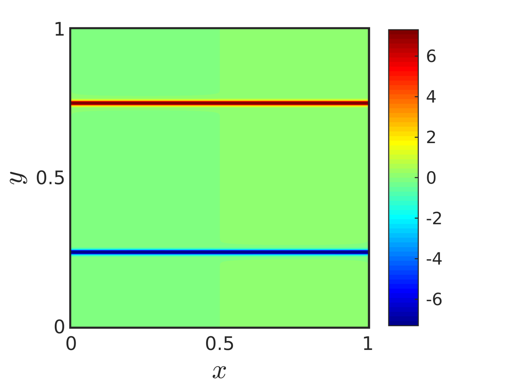
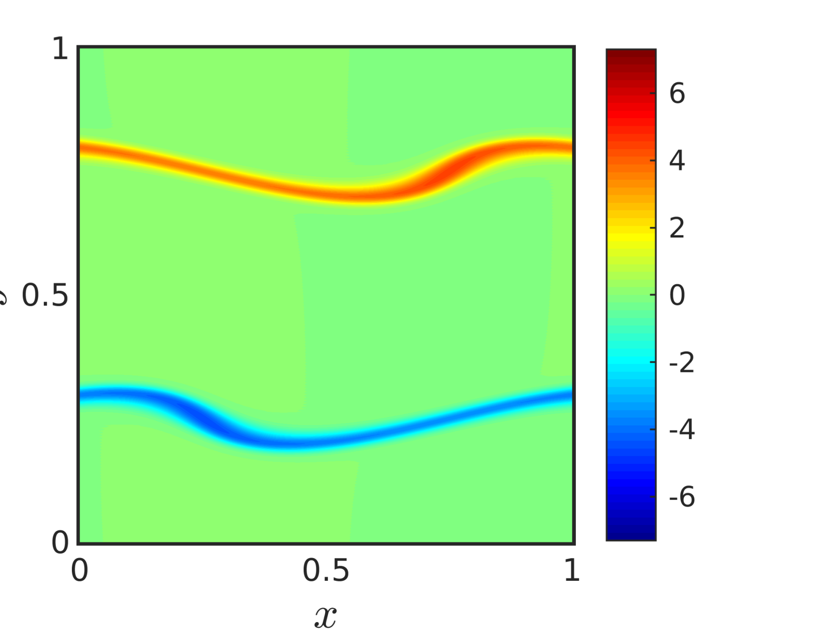
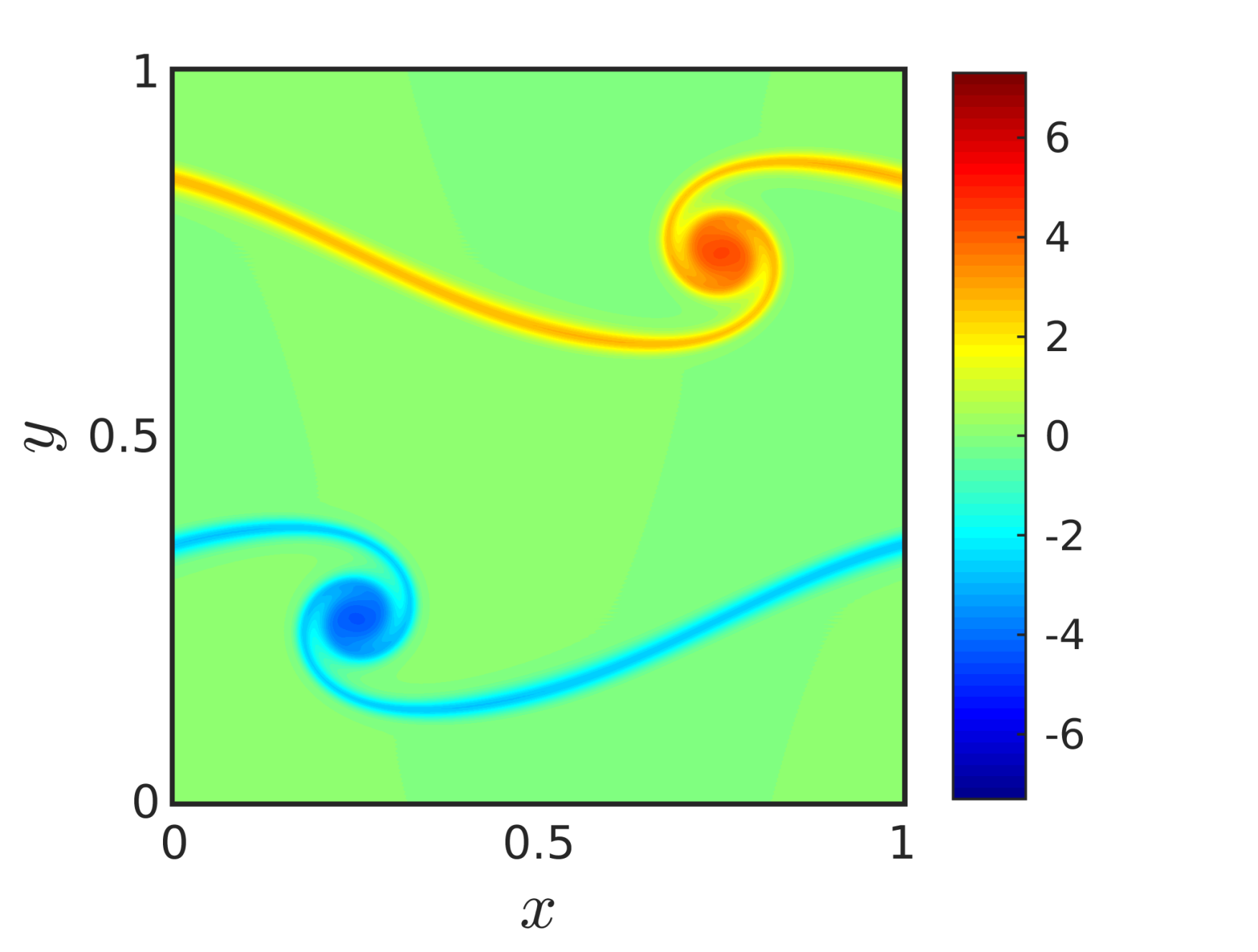
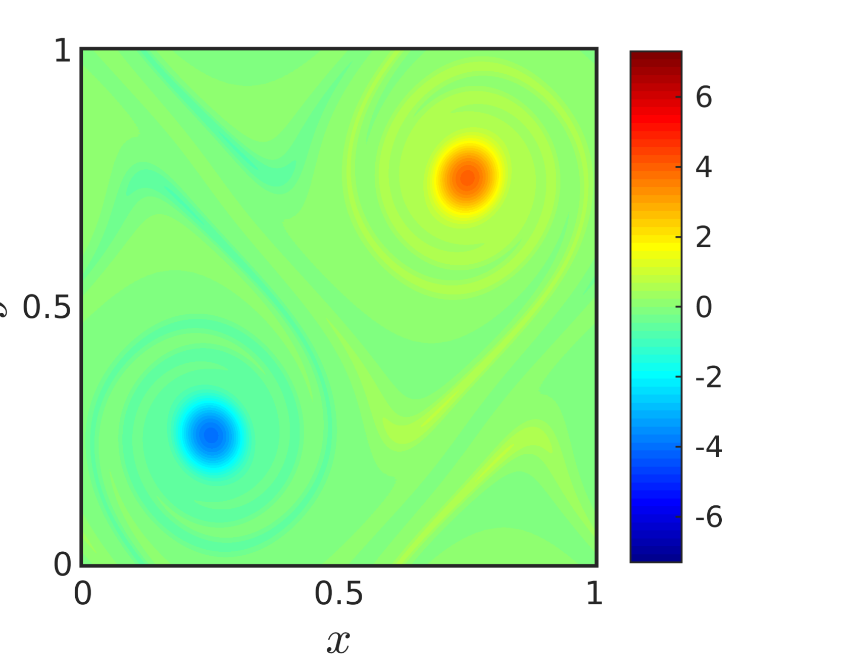
Figure 1: Spatial distribution of $\omega_{z}/\sqrt{\Omega_{ref}}$ for case $r160$ at 4 instants $t\sqrt{\Omega_{ref}}=\{0,7,10,23\}$ in the following respective order: top left, top right, bottom left and bottom right.

The incompressible 2D Navier-Stokes equations are solved with the initial and boundary conditions outlined above using JAGUAR on a structured mesh with $72\times 72$ square elements. The Mach number ($Ma$) is set to zero to approach, as much as possible, incompressibility. The solution and flux points are located following Gauss-Lobatto-Chebyshev and Legendre collocation, respectively, and the CFL is kept constant at 0.5. The fluxes at the cell faces are computed with the Roe scheme. The temporal integration is done with a six-stage, fourth-order low-dissipation low-dispersion Runge-Kutta scheme optimized for the spectral difference code using the procedure in [5]. We use an in-house, fully spectral code (MatSPE) designed for periodic incompressible viscous flows to solve the same test case and validate JAGUAR. The output of the two codes is compared on Figure 2, showing that the agreement between the codes is extremely good.

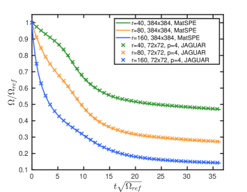
Figure 2: Evolution of $\Omega(t)$ at 3 different values of $r$, JAGUAR vs. fully spectral and incompressible code MatSPE. The legend includes the number of Fourier modes used in each direction for the MatSPE simulation (of which 1/3 are zero-padded for dealiasing), while the JAGUAR data includes parameter $p$ which is the selected order of the spatial discretization of the spectral difference scheme. The grid used in the JAGUAR simulation is a $72\times 72$ structured mesh which, together with the setting $p=4$, yields $360$ degrees of freedom (DoF) per spatial direction. So we are effectively comparing $256^{2}$ DoF with MatSPE against $360^{2}$ DoF with JAGUAR.

We define the following cost function

$$J = \int_{0}^{T}\Omega(t)\ dt.$$ (8)

Its derivative with respect to $r$ will be the target sensitivity we compute by means of AD. From a physical point of view, $\Omega(t)$ is directly proportional to the rate of kinetic energy dissipation in the flow due to the action of viscosity. Hence, the area under a curve of $\Omega(t)$ on Figure 2 for a given time interval is a proxy for the kinetic energy dissipated by the flow during that time. It may be argued that since our numerical experiments only target $dJ/dr$, it is pointless to use adjoint-mode AD because $r$ is a scalar. One must bear in mind, however, that the final application of our study is to compute sensitivities of some $J$ with respect to many inputs. Restricting the number of inputs to one in the sequel is only a convenient way to validate our proposed work flow and the AD derivatives, as well as to compare and study performance.

The computation of $J$ in the primal code is carried out by adding a contribution to the time integral at each new time step in a running sum fashion, using a simple trapezoidal rule. The tangent-differentiated code accumulates contributions of each time step to $dJ/dr$, along with the primal time-stepping sequence, i.e. in the same order. This is conceptually simple: once we reach the iteration corresponding to $t=T$ (which we will call iteration number $N$), both $J$ and $dJ/dr$ are known and the program can end. In contrast, the adjoint-differentiated code will first run an initial forward sweep that will integrate the Navier-Stokes equations from $t=0$ to iteration $N$ of the time-stepping loop, chiefly to generate the final state of the program variables. Only then can the backward sweep of the adjoint code start to accumulate derivatives, computing the sensitivity of $J$ with respect to the state variables at iteration $N-1$, and carry on stepping back in time to finally obtain $dJ/dr$ when $t=0$ is reached. In order to provide intermediate values from the forward sweep to the backward sweep in the correct order (i.e. reversed), a combination of stack storage and additional forward recomputation is needed, making a good checkpointing scheme essential. The recomputations and stack use will inevitably imply that one run of the adjoint code requires significantly more memory and execution time than the tangent code. We thus expect the tangent code to still outperform the adjoint code when $p=q$ or when $q$ is only a few times larger than $p$, but the adjoint code will definitely outperform the tangent code when $p\ll q$, which is the case in many applications.

3.2 Inviscid compressible flow over an airfoil section

We study the two-dimensional flow around a NACA 0012 airfoil at zero angle of attack $\alpha$. It is a symmetric airfoil commonly used as an aerodynamics test case. Even though the flow eventually becomes stationary, JAGUAR is run in unsteady mode so that the steady state is reached without numerical stabilization. Two important differences with respect to the previous test case deserve to be highlighted: the flow is compressible and there is no viscosity in the set of equations solved by JAGUAR. We consider two levels of compressibility: close to incompressible with $Ma=0.1$, and a higher subsonic regime with $Ma=0.5$. Both are below the critical Mach number, so no shock appears on the upper side of the airfoil. Yet at $Ma=0.5$, we expect to see sizable departures from predictions based on two-dimensional, incompressible and inviscid (i.e. potential) flow predictions. The domain is discretized with a structured mesh of 2876 quadrilateral elements. We are interested in the derivative of the lift coefficient $Cl$ with respect to $\alpha$ at $\alpha=0^{\circ}$. This frequently computed quantity allows for comparison with experimental measurements [26] and with numerical computations based on the potential flow solver XFOIL [9]. Figure 3 shows the Mach number distribution around the airfoil for the angle of attack $\alpha=4^{\circ}$, computed by JAGUAR with the same mesh as the $\alpha=0^{\circ}$ case. At this $\alpha$ setting, an asymmetric pressure distribution gives rise to lift due to the faster flow on the upper side – yet subsonic conditions are mantained.

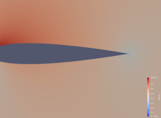
Figure 3: Distribution of the Mach number around a NACA 0012 airfoil section at $\alpha=4^{\circ}$, computed with JAGUAR in inviscid two-dimensional mode. The upstream Mach number is $Ma=0.5$, the flow is from left to right.

3.3 Sensitivity validations with finite differences

The estimates of a given sensitivity computed with tangent- or adjoint-mode AD codes should agree almost to machine precision, as they result from the same computation modulo associativity-commutativity. In contrast, the reference value against which to validate the sensitivity is obviously a finite-difference (FD) estimate, which is subject to errors due to the contribution of higher derivatives. For the viscous test case, we compute our FD estimates with two independent realizations at $r$ and $r+dr$, where $dr/r=10^{-5}$. Similarly, for the inviscid test case we use two independent realizations at $\alpha$ and $\alpha+d\alpha$, where $d\alpha/\alpha=10^{-5}$. We thus expect an agreement between FD and AD derivatives up to more or less half of the decimals, whereas we expect a much better agreement between tangent AD and adjoint AD derivatives.

4 Differentiation work flow

We adopted the following work flow with regards to the JAGUAR flow solver, the working principles of Tapenade and the Adjoinable MPI library:

• Identify the part of the code that computes the function to differentiate, exactly from the differentiation input variables to the differentiation output, and make it appear as a procedure (the “head” procedure of section 2.4). This may require a bit of code refactoring. The differentiation tool must be given (at least) this root procedure and the call tree below it.

• Migrate all MPI calls to Adjoinable MPI, whether AD will be applied in tangent or in adjoint mode. This involves two steps. First, as Adjoinable MPI does not support all MPI communication styles (e.g. one-sided), the code must be transformed to only use the supported styles, which is a reasonably large subset. Second, effectively translate the MPI constructs into their Adjoinable MPI equivalent, which occasionally requires minor modifications to the call arguments. As Adjoinable MPI is just a wrapper around MPI, the resulting code should still compile and run, and it is wise to test that.

• Provide the AD tool with the source of the head procedure and of all the procedures that it may recursively call, together with the specification of the differentiation input and output variables. Then differentiate, after which two steps follow. First, fix all issues signaled by the AD tool, e.g. unknown external procedures or additional info needed, and validate the differentiated code. Second, address performance issues and in particular optimize the checkpointing strategy by adding AD-related directives to the source. This may also involve special treatment of linear algebra procedures such as solvers.

Step A) is best illustrated with the viscous test case. The main program in JAGUAR calls thirteen procedures before $r$ is used to initialize the velocity field. $r$ has thus no impact on the code prior to the velocity field initialization. A few procedure calls after the initialization, the time integration routine is called, at the end of which $J$ is known. All code after that point has no impact on the sensitivity computation we investigate. So we create a head that contains all procedure calls from the velocity field initialization to the time integration routine, excluding everything else. This head, say TopSub(X,Y), takes $X=r$ as input and outputs $Y=J$. It will be differentiated in step C).

The work involved in step B) is likely to depend heavily on the primal code and the state of advancement in the Adjoinable MPI project at the time of implementation. Codes tuned for high-performance computing which repeat a non-blocking communication pattern many times benefit from using persistent communication requests through the MPI_SEND_INIT and MPI_SEND_RECV calls. This leads to the later use of the MPI_STARTALL and MPI_WAITALL constructs when the communications are actually invoked. These communication patterns are not currently supported by the Adjoinable MPI library, and the advice of the developers in such cases is to replace them by loops over processes containing individual non-blocking MPI_ISEND, MPI_IRECV and their respective MPI_WAIT calls. The output of the modified primal code needs to be validated against the original version, which can be done reliably on a small number of processes. The impact of the modifications on the performance, however, is difficult to assess without access to hundreds, preferably thousands of cores. With 16 cores, we record a performance drop of $2.6\%$ after $3.5\times 10^{5}$ time steps on the inviscid test case. Since the modified code preserves the non-blocking structure of the original code, we expect the performance drop to be low. The drop should be attributed to the overhead for communication between the process and the communication controller, which is what persistent communications alleviate - and not between one communication controller and another. All in all, support for persistent communications would be a useful addition to the Adjoinable MPI library.

Migrating from MPI to Adjoinable MPI involves changes that are mainly cosmetic. The name of each MPI call requires relabeling to match the name of the Adjoinable MPI wrapper for that call. Typically, all that needs to be done is to change CALL MPI_COMM_SIZE, CALL MPI_BARRIER, CALL MPI_ALLREDUCE, etc. into CALL AMPI_COMM_SIZE, CALL AMPI_BARRIER, CALL AMPI_ALLREDUCE and so on. These modifications can be automated with a suitable script. For each point-to-point Adjoinable MPI call, however, the user has to manually add an argument that specifies the kind of MPI call at the other end of the communication. For example, the extra argument for a send instruction may be AMPI_TO_RECV, AMPI_TO_IRECV_WAIT or AMPI_TO_IRECV_WAITALL. Similarly, the extra argument for a receive may be AMPI_FROM_SEND, AMPI_FROM_ISEND_WAIT, AMPI_FROM_ISEND_WAITALL. This must be left to the programmer, as no static data-flow analysis can determine it in general.

In step C), specific instructions can be passed on to tune how Tapenade should handle the checkpointing of the primal code. The most important part in specifying these is to identify the time-stepping loop(s), to label them for binomial checkpointing, and to assign them a well-chosen number of snapshots. It can be done by placing a number of specific directives in the source code, to indicate which subroutine calls should be checkpointed portions. By default, all of them are. This is a delicate trade off, of experimental nature. The rule of thumb is to avoid checkpointing on “small” procedures, as they require very little space on stack and on the other hand may require a large snapshot for checkpointing. Typically a subroutine that takes in an array and an index to just overwrite the array element at this index is considered “small” and should not be checkpointed. A case of forbidden checkpointing, detailed in [15], is a subroutine that contains one end of a non-blocking communication, for example the MPI_ISEND or the MPI_IRECV, but not the corresponding MPI_WAIT. The subroutine is not reentrant and must not be checkpointed. In our application, this happened on two procedures. For completeness, we must point out a manual modification required on the adjoint code, i.e. after step C). At the “turning” point between forward and backward sweeps, one must insert specific calls to declare, for each primal variable V that is active (i.e. it has a derivative) and that is passed through MPI, the correspondence with its derivative counterpart Vb. Specifically, this is done by calling ADTOOL_AMPI_Turn(V, Vb). This must be done by hand, until Tapenade generates these calls automatically.

The differentiation of the head routine TopSub(X,Y) leads to TopSub_d(X,Xd,Y,Yd) in tangent mode and to TopSub_b(X,Xb,Y,Yb) in adjoint mode. The final program calls the differentiated routines when derivatives are needed. In doing so, it is necessary to correctly set the initial Xd (respectively Yb) and to correctly interpret the resulting Yd (resp. Xb). For parallel execution specifically, the full sensitivity could be spread across the Xb of several processes after having seeded all of them with Xb=0 and Yb=1. In such cases, a global reduction operation is needed to sum the resulting Xb held by each process in order to recover the correct sensitivity. Strategies for handling the dispersion of the derivatives across different processes in adjoint-mode AD have been discussed in [29].

Let us finally comment on our experience using an AD tool on a large parallel code. The difficulties encountered on the AD tool side, including 3 bug reports, will no longer stand on the way of future attempts at performing a similar study. This gives a rough idea of the maturity, or lack thereof, of the Tapenade tool. Issues with the Adjoinable MPI library were limited to the lack of support, at the time of writing, for persistent communication requests. The fact that Tapenade does not yet introduce automatically the needed calls to ADTOOL_AMPI_Turn is a limitation. We would like to think that having one developer of the AD tool among us is not a prerequisite for success. The three bugs mentioned above were fixed after being reported by email. Performance tuning of the adjoint code is not yet optimal, and we believe this calls for better support from the AD tool for choosing a good checkpointing scheme.

5 Results

5.1 Viscous double shear layer

Differentiation method	Sensitivity $(dJ/dr)$
FD (MPI)	-0.22002254
Tangent AD (AMPI)	-0.22002394265381
Adjoint AD (AMPI)	-0.22002394265861

Table 2: $dJ/dr$ computed with three different methods, for the time integration interval between $t=0$ and $t=T$ ($6.8\times 10^{5}$ time steps). Viscous test case with $r=160$, run on 16 parallel processes.

The temporal integration of the equations of motion is carried out from $t=0$ to the $n-th$ iteration of the time integration loop in JAGUAR, with $n=6.8\times 10^{5}$. With the CFL setting outlined in section 3, this number of time steps corresponds to $t\sqrt{\Omega_{ref}}=19.8$, which from Figure 1 can be seen as the time when the decay of $\Omega$ becomes slow for all three values of $r$. The value of $dJ/dr$ is given in Table 2, where the results from FD, tangent-mode AD and adjoint-mode AD are all gathered. The agreement between FD-based sensitivities and AD validates the differentiation procedure. In particular, we note that although the underlying system is unsteady and results from non-linear equations, there is no breakdown of the conventional sensitivity analysis. It is important to emphasize this because, as illustrated by [6] for the Lorentz attractor, unsteadyness and chaos can undermine sensitivity computations and motivate the use of more complex approaches. But our system, although unsteady and non-linear, does not fall into the category of problems that require these approaches.

The agreement between the two AD-based sensitivities is excellent, within round-off error of double precision arithmetic. It was expected in case of correct differentiation by Tapenade, but nevertheless it is puzzling when comparing the drastic differences between the two differentiated codes. The fact that the adjoint-differentiated code outputs the correct answer after carrying out the time-stepping loop backwards confirms the absence of any stability or convergence issues related to inverting the instructions of a code that integrates in time an irreversible and dissipative system. More specifically, there is no issue of numerical instability caused by a term with negative diffusivity.

The time required for the various computations is shown on Table 3. A factor of two is indicated for the FD computation, given that two runs of the primal code are required. The computations are run on 16 Intel(R) Xeon(R) Gold 6140 processors at 2.30GHz. The Intel Fortran compiler version 18.0.2 is used, with identical optimization flags for all codes: -ipo -O3. The Intel MPI Library was used for the MPI implementation, in its 2018 version. It appears that the tangent-mode AD can be faster than two runs of the primal code, requiring 1.7 times the execution time of the primal code. The higher accuracy of sensitivity computations from tangent-mode AD thus comes with the added benefit of a faster computation than that of FD. Furthermore, each additional cost function differentiated with respect to $r$ will require an additional FD computation, whereas the cost of each new sensitivity with respect to $r$ will keep the cost of the tangent-mode execution constant. We note in passing that the FD computation is based on the MPI code before the modifications of step B) outlined in section 4, so that the tangent-mode AD is faster than the FD computations despite the move from MPI to Adjoinable MPI. This indicates that the cost of this additional wrapper on top of the MPI library is negligible.

Differentiation method	Normalized compute time
FD (MPI)	$1\>(\times 2)$
Tangent AD (AMPI)	$1.7$
Adjoint AD (AMPI)	$15.4$

Table 3: Same as Table 2, but showing execution times normalized by the primal code execution time. Viscous test case, run on 16 parallel processes.

Table 3 also shows the slowdown factor of the adjoint code, which is 15.4 and deserves some discussion. An initial experiment without any specific checkpointing scheme simply ran out of memory after only less than a hundred time-stepping iterations. Therefore, binomial checkpointing is unavoidable. It accounts for a significant part of this adjoint slowdown: since we chose to allow for 80 snapshots for binomial reversal of $6.8\times 10^{5}$ time steps, the binomial model tells us this costs an average 3.9 extra recomputations per time step. This leaves us with roughly an 11–fold slowdown to account for, which is still higher than expected. By far the most expensive task in JAGUAR is the computation of the right-hand side of the governing equations, required six times per time step by calling procedure ComputeRhsNavier. The latter can itself be decomposed into eight subroutines, shown on Figure 4.

⬇

SUBROUTINE ComputeRhsNavier

CALL ExtrapolSolAndComputeFlux

CALL Scatter

CALL RiemannSolver

CALL GatherSolution

CALL GradientAndInternalFlux

CALL ViscousFlux

CALL GatherFlux

CALL FluxDivAndUpdate

END SUBROUTINE ComputeRhsNavier

Figure 4: Breakdown of the most computationally-expensive subroutine in the code, ComputeRhsNavier.

Upon differentiation in adjoint mode, the subroutines within ComputeRhsNavier will lead to adjoint versions, such as ExtrapolSolAndComputeFlux_b, Scatter_b, etc. Table 4 contains the slowdown factor for each individual adjoint subroutine found inside ComputeRhsNavier compared to its original version.

subroutine	adjoint/primal slowdown
ExtrapolSolAndComputeFlux	2.35
Scatter	1.69
RiemannSolver	8.45
GatherSolution	2.56
GradientAndInternalFlux	12.84
ViscousFlux	6.44
GatherFlux	1.73
FluxDivAndUpdate	5.60

Table 4: Slowdown factor between original and adjoint versions of the subroutines within ComputeRhsNavier. None of the routines above include parallel communication calls within them.

$54\%$ of the time taken by ComputeRhsNavier is spent during execution of GradientAndInternalFlux, so that the largest slowdown – almost 13 – occurs precisely within the most expensive routine. Calls to push and pop intermediate values into the AD stack are spread across all eight procedures, and for this reason we cannot ascribe the performance penalty incurred specifically in GradientAndInternalFlux to AD stack access only. However, we do note that improving the performance when reading and writing into the AD stack – which happens regardless of binomial checkpointing – will generally have a direct impact on adjoint-differentiated code speed. Future efforts on the AD tool side will be geared in that direction.

The type of information on Table 4 provides the AD user with indications on where to hand-tune the AD process further – by preventing some procedures from being checkpointed, for instance. But from here onwards, the process is no longer automatic and will depend heavily on the specific code under consideration. We therefore limit our study to the performance obtained “out of the box” with the current degree of maturity in the development of the AD tool, which has undergone major improvements over the years to reach its present state. With the obtained performance, the adjoint code is already preferable to the tangent code as soon as the number of input variables, with respect to which we request sensitivities, goes over 15.

5.2 Inviscid compressible flow around an airfoil

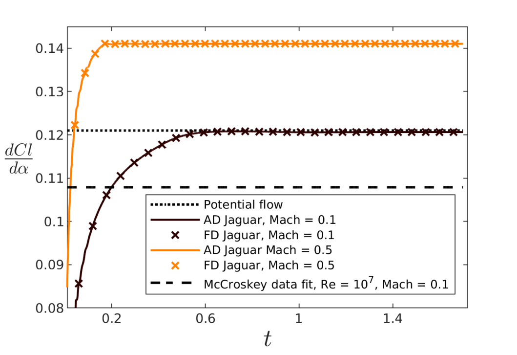
Figure 5: Sensitivity of the lift coefficient $Cl$ to a change in incidence angle $\alpha$ around a NACA 0012 airfoil at zero incidence. Two Mach numbers considered, sensitivities computed with FD and JAGUAR differentiated in tangent-mode AD. Values are compared with the curve fit to experimental data from [26], and with the solution found using FD with the panel code XFOIL (potential flow). Time $t$ is in code units. We verified that the agreement between the JAGUAR output at $Ma=0.1$ and $Ma=0.5$ is considerably improved if normalized by the low $Ma$ correction factor $\sqrt{1-(Ma)^{2}}$.

The flow around the airfoil converges to a steady state after integrating the governing equations for long enough. It can be seen on Figure 5 that both the FD approximation and the AD computation (only tangent-mode used) exhibit similar time-dependence during an initial transient phase, and then stabilize around a converged value. The FD and AD computations agree across both Mach numbers and throughout the time interval considered, validating the AD code. We also show the value obtained for the sensitivity using an altogether different code (XFOIL) and applying FD to it around the same airfoil geometry and for an angle of attack $\alpha=0$. The experimental curve fit shown on Figure 5 is for comparison, illustrating that the discrepancy between the various estimations of the same quantity is within reasonable bounds considering the difference between the approaches.

The time span on Figure 5 by the JAGUAR computations represents $4.3\times 10^{5}$ and $1.2\times 10^{6}$ time steps with Mach=0.1 and 0.5, respectively, using a CFL of 0.5 in both cases. The tangent-mode AD computations last 1.6 times the execution time of the corresponding primal code for both Mach numbers. For this test case, the computations are run on 27 Intel® Xeon(R) Silver 4110 processors at 2.10GHz, with the Intel Fortran compiler version 15.0.1 and identical optimization flag for primal and AD codes: -O3. MPICH-3.2 was used. It is interesting to see that the ratio of run times between the tangent-differentiated and the primal code is very close to that obtained for the previous test case, which was 1.7. The primal codes of both test cases differ due to the presence of additional code lines related to the viscous stresses.

6 Conclusions and future work

A CFD code with an optimized parallel communications layer has been automatically differentiated by letting the AD tool handle the communications layer in an automated way. In adjoint mode the inversion of the communications during the backward sweep was found to produce correct code which could execute in 15 times the primal code execution time. The computational overhead is to a large extent the consequence of having to resort to binomial checkpointing to trade storage for computational time in order to invert a temporal integration loop with a number of iterations of the order of $10^{6}$. We have presented a detailed outline of the code modifications required to achieve the correct differentiation of the parallel code. Two flows were solved with the CFD code, an inviscid and a viscous test case. The latter is a physically dissipative system, which has been computed using the backward mode of AD without running into stability issues and yielding the correct derivative at the end of the computation. Both test cases exhibited run times for the tangent-differentiated codes which were in the range 1.6-1.7 times slower than a single primal code run. They are therefore readily superior to finite difference approximations even for single derivative computations. A natural further step would involve embedding the derivative solver into an optimal control loop. The strength of a code such as JAGUAR lies in its ability to handle acoustics problems, such as the noise radiated by the wake of an object during a given time. Optimization in this type of time-dependent and multi-parameter applications is the subject of ongoing work.

7 Acknowledgments

This work has been financed by a grant from the STAE Foundation for the 3C2T project, managed by the IRT Saint-Exupéry. J.I.C. acknowledges funding from the People Program (Marie Curie Actions) of the European Union’s Seventh Framework Program (FP7/2007-2013) under REA grant agreement n. PCOFUND-GA-2013-609102, through the PRESTIGE program coordinated by Campus France. The computations for the viscous test case were carried out at the CALMIP computing center under the project P0824.

References

- [1] T.A. Albring, M. Sagebaum, and N.R. Gauger. Efficient aerodynamic design using the discrete adjoint method in SU2. In 17th AIAA/ISSMO multidisciplinary analysis and optimization conference, page 3518, 2016.
- [2] American Society of Mechanical Engineers Digital Collection. Comparison of various CFD codes for LES simulations of turbomachinery: from inviscid vortex convection to multi-stage compressor, volume 2C: Turbomachinery, 2018.
- [3] G. Aupy and J. Herrmann. Periodicity in optimal hierarchical checkpointing schemes for adjoint computations. Optimization Methods and Software, 32(3):594–624, 2017.
- [4] G. Aupy, J. Herrmann, P. Hovland, and Y. Robert. Optimal multistage algorithm for adjoint computation. SIAM Journal on Scientific Computing, 38(3):C232–C255, 2016.
- [5] J. Berland, C. Bogey, and C. Bailly. Low-dissipation and low-dispersion fourth-order Runge–Kutta algorithm. Computers & Fluids, 35(10):1459–1463, 2006.
- [6] P.J. Blonigan, Q. Wang, E.J. Nielsen, and B. Diskin. Least-squares shadowing sensitivity analysis of chaotic flow around a two-dimensional airfoil. AIAA Journal, 56(2):658–672, 2018.
- [7] A. Cassagne, J.F. Boussuge, N. Villedieu, G. Puigt, I. D’ast, and A. Genot. Jaguar: a new CFD code dedicated to massively parallel high-order LES computations on complex geometry. In The 50th 3AF International Conference on Applied Aerodynamics (AERO 2015), 2015.
- [8] I. Charpentier. Checkpointing schemes for adjoint codes: application to the meteorological model Meso-NH. SIAM Journal on Scientific Computing, 22(6):2135–2151, 2001.
- [9] M. Drela. Xfoil: An analysis and design system for low reynolds number airfoils. In Thomas J. Mueller, editor, Low Reynolds Number Aerodynamics, pages 1–12, Berlin, Heidelberg, 1989. Springer Berlin Heidelberg.
- [10] Sebastian Götschel and Martin Weiser. Lossy compression for pde-constrained optimization: adaptive error control. Computational Optimization and Applications, 62(1):131 – 155, 2015.
- [11] A. Griewank. Achieving logarithmic growth of temporal and spatial complexity in reverse automatic differentiation. Optimization Methods and Software, 1(1):35–54, 1992.
- [12] A. Griewank and A. Walther. Evaluating derivatives: principles and techniques of algorithmic differentiation, volume 105. Siam, 2008.
- [13] J. Grimm, L. Pottier, and N. Rostaing-Schmidt. Optimal time and minimum space-time product for reversing a certain class of programs. In M. Berz, C. Bischof, and A. Griewank, editors, Computational differentiation, techniques, applications, and tools, pages 95–106, Philadelphia, 1996. SIAM.
- [14] L. Hascoët and V. Pascual. The Tapenade automatic differentiation tool: principles, model, and specification. ACM Transactions on Mathematical Software (TOMS), 39(3):20, 2013.
- [15] L. Hascoët and J. Utke. Programming language features, usage patterns, and the efficiency of generated adjoint code. Optimization Methods and Software, 31(5):885–903, 2016.
- [16] P. Heimbach, C. Hill, and R. Giering. Automatic generation of efficient adjoint code for a parallel Navier-Stokes solver. In Computational Science ICCS 2002, pages 1019–1028, Berlin, Heidelberg, 2002. Springer Berlin Heidelberg.
- [17] P. Heimbach, C. Hill, and R. Giering. An efficient exact adjoint of the parallel mit general circulation model, generated via automatic differentiation. Future Generation Computer Systems, 21(8):1356–1371, 2005.
- [18] P. Hovland and C. Bischof. Automatic differentiation for message-passing parallel programs. In Proceedings of the First Merged International Parallel Processing Symposium and Symposium on Parallel and Distributed Processing, pages 98–104, March 1998.
- [19] J.C. Hückelheim, L. Hascoët, and J.D. Müller. Algorithmic differentiation of code with multiple context-specific activities. ACM Trans. Math. Softw., 43(4):35:1–35:21, January 2017.
- [20] J.C. Hückelheim, P.D. Hovland, M.M. Strout, and J.-D. Müller. Parallelizable adjoint stencil computations using transposed forward-mode algorithmic differentiation. Optimization Methods and Software, 33(4-6):672–693, 2018.
- [21] A. Jameson. A proof of the stability of the spectral difference method for all orders of accuracy. Journal of Scientific Computing, 45(1-3):348–358, 2010.
- [22] D. Jones, J.J. Müller, and F. Christakopoulos. Preparation and assembly of discrete adjoint CFD codes. Computers & Fluids, 46(1):282–286, 2011. 10th ICFD Conference Series on Numerical Methods for Fluid Dynamics (ICFD 2010).
- [23] G.K.W. Kenway, C.A. Mader, P. He, and J.R.R.A. Martins. Effective adjoint approaches for computational fluid dynamics. Progress in Aerospace Sciences, page 100542, 2019.
- [24] D.A. Kopriva. A staggered-grid multidomain spectral method for the compressible navier–stokes equations. Journal of computational physics, 143(1):125–158, 1998.
- [25] Yen Liu, Marcel Vinokur, and Zhi Jian Wang. Spectral difference method for unstructured grids I: basic formulation. Journal of Computational Physics, 216(2):780–801, 2006.
- [26] W.J. McCroskey. Technical evaluation report on the fluid dynamics panel symposium on applications of computational fluid dynamics in aeronautics. NASA STI/Recon Technical Report N, 87, 1987.
- [27] J.D. Müller, J.C. Hückelheim, and O. Mykhaskiv. STAMPS: a finite-volume solver framework for adjoint codes derived with source-transformation AD. In 2018 Multidisciplinary Analysis and Optimization Conference, page 2928, 2018.
- [28] M. Sagebaum, T. Albring, and N.R. Gauger. High-performance derivative computations using CoDiPack. arXiv preprint arXiv:1709.07229, 2017.
- [29] M. Schanen. Semantics driven adjoints of the message passing interface. PhD thesis, Universitätsbibliothek der RWTH Aachen, 2016.
- [30] M. Schanen, M. Förster, and U. Naumann. Second-order algorithmic differentiation by source transformation of MPI code. In European MPI Users’ Group Meeting, pages 257–264. Springer, 2010.
- [31] M. Schanen and U. Naumann. A wish list for efficient adjoints of one-sided MPI communication. In European MPI Users’ Group Meeting, pages 248–257. Springer, 2012.
- [32] M. Schanen, U. Naumann, L. Hascoët, and J. Utke. Interpretative adjoints for numerical simulation codes using mpi. Procedia Computer Science, 1(1):1825–1833, 2010.
- [33] M. Towara, M. Schanen, and U. Naumann. MPI-parallel discrete adjoint openfoam. Procedia Computer Science, 51:19–28, 2015.
- [34] J. Utke, L. Hascoët, P. Heimbach, C. Hill, P. Hovland, and U. Naumann. Toward Adjoinable MPI. In 2009 IEEE International Symposium on Parallel Distributed Processing, pages 1–8, May 2009.
- [35] K. Van den Abeele, C. Lacor, and Z.J. Wang. On the stability and accuracy of the spectral difference method. Journal of Scientific Computing, 37(2):162–188, 2008.
- [36] J. Vanharen, G. Puigt, X. Vasseur, J.F. Boussuge, and P. Sagaut. Revisiting the spectral analysis for high-order spectral discontinuous methods. Journal of Computational Physics, 337:379–402, 2017.
- [37] A. Walther and A. Griewank. Advantages of binomial checkpointing for memory-reduced adjoint calculations. In Numerical mathematics and advanced applications, pages 834–843. Springer, 2004.
- [38] F.D. Witherden and A. Jameson. Future directions in computational fluid dynamics. In 23rd AIAA Computational Fluid Dynamics Conference, page 3791, 2017.
- [39] S. Xu, Radford D., M. Meyer, and J.D. Müller. Stabilisation of discrete steady adjoint solvers. Journal of Computational Physics, 299:175–195, 2015.