Utility Mining Across Multi-Sequences with Individualized Thresholds

Abstract.

Utility-oriented pattern mining has become an emerging topic since it can reveal high-utility patterns (e.g., itemsets, rules, sequences) from different types of data, which provides more information than the traditional frequent/confident-based pattern mining models. The utilities of various items are not exactly equal in realistic situations; each item has its own utility or importance. In general, user considers a uniform minimum utility (minutil) threshold to identify the set of high-utility sequential patterns (HUSPs). This is unable to find the interesting patterns while the minutil is set extremely high or low. We first design a new utility mining framework namely USPT for mining high-Utility Sequential Patterns across multi-sequences with individualized Thresholds. Each item in the designed framework has its own specified minimum utility threshold. Based on the lexicographic-sequential tree and the utility-array structure, the USPT framework is presented to efficiently discover the HUSPs. With the upper-bounds on utility, several pruning strategies are developed to prune the unpromising candidates early in the search space. Several experiments are conducted on both real-life and synthetic datasets to show the performance of the designed USPT algorithm, and the results showed that USPT could achieve good effectiveness and efficiency for mining HUSPs with individualized minimum utility thresholds.

1. Introduction

Sequential pattern mining (SPM) (Agrawal and Srikant, 1995; Srikant and Agrawal, 1996; Pei et al., 2001) has become an interesting and emerging issue in knowledge discovery in databases (KDD) (Agrawal et al., 1993; Chen et al., 1996), and it has been used in many real-life applications, such as behavioral analysis of customers, DNA sequence analysis, and natural disaster analysis (Fournier-Viger et al., 2017). The purpose of SPM is to discover the frequent sequences from the sequence database using a uniform users’ defined minimum threshold. Both SPM and frequent itemset mining (FIM) (Agrawal et al., 1994; Han et al., 2004) are frequent pattern mining approaches, where the main difference between them is that the processed data in SPM is consequentially time-ordered. Thus, it is more complicated and complex to discover the interesting information from the sequential databases in SPM.

The frequency-based pattern mining frameworks (e.g., FIM and SPM) mainly consider the co-occurrence frequencies of the itemset/sequence. The above well-known frameworks cannot, however, retrieve the high-utility patterns or handle more important factors for pattern mining, such as interestingness, utility, importance, and risk. To solve this limitation, in recent decades, the utility-oriented pattern mining framework (Gan et al., 2019c) named high-utility itemset mining (HUIM) has been extensively studied and successfully applied in numerous domains (Chan et al., 2003; Tseng et al., 2013; Liu et al., 2005). HUIM considers the quantity and unit utility of items to measure the high-utility itemsets (HUIs) from a quantitative dataset. Traditional HUIM does not hold the downward closure property (Agrawal et al., 1994), and it becomes a non-trivial task to mine the useful and meaningful HUIs from the databases.

Although HUIM is useful to discover high-utility patterns in many real-life applications, it cannot handle a sequence database that contains the embedded timestamp information of the events/items. In particular, the ordering of elements or events is important in many real-life domains. For instance, HUIM can be applied to analyze the shopping behaviors of the customers for targeted marketing and also be utilized for the recommendation task since the order of purchase products should be considered to retrieve more interesting patterns. Besides, the events/sequences in sequential data commonly contain multiple time-order sequences, but not a single long sequence. For example, the real dataset in market basket analysis is usually has rich information, including user ID, timestamp, event ID, record (event), quantity, and unit price. In general, each record in these datasets contains multi-sequences. Episode mining (Mannila et al., 1997) focuses on discovering interesting patterns from a single sequence, while SPM (Agrawal and Srikant, 1995; Srikant and Agrawal, 1996; Pei et al., 2001; Fournier-Viger et al., 2017) usually discovers frequent sequences from multi-sequences. To solve the above limitation, high-utility sequential pattern mining (HUSPM) (Lan et al., 2014; Wang et al., 2016; Yin et al., 2012, 2013) was introduced, and it mainly aims at discovering more informative sequential patterns. It is more complicated than HUIM and SPM since both the ordering and the utility of events or elements are considered together. A sequence is considered to be a high-utility sequential pattern (HUSP) if its overall utility is no less than a user-specified minimum utility threshold. To retrieve HUSPs, several techniques and approaches have been developed in the past (Alkan and Karagoz, 2015; Wang et al., 2016; Yin et al., 2012). However, most of these techniques focus on improving the mining efficiency, but not its effectiveness. In addition, all the existing HUSPM approaches suffer from an important limitation since most of them focus on mining the HUSPs with a uniform and single minimum utility threshold. Thus, all the items and sequences are considered as being the same weight or importance, which is unfair and not realistic in some real-life situations.

In real-life situations, each object/item has its own importance and utility because the utility (e.g., risk, profit) for various objects/items are not exactly equal. Some patterns with higher importance may have low utilities in databases. For example, a shopping mall contains more than hundred or thousand products, and it is impossible to measure them with the same importance due to their characteristics. For instance, diamond and clothe are two different products and should not be treated as the same importance. It is more reasonable to respectively set different utility thresholds for diamond and clothe since they have different features. Although there are numerous studies of market basket analysis focusing on SPM from the sequential purchase data, none of them consider the quantity, utility factor, or individuality of importance at the same time. Another example can be referred to the recommendation system, which utilizes time-stamp information to improve the performance. A lower threshold could be set for a target topic or product that users are interested to reveal more information, or to sell multiple products for mixed bundling.

Therefore, mining HUSPs with an individualized threshold of each item is more realistic than existing HUSPM algorithms for retrieving more useful and meaningful patterns. However, it is not a trivial task to address these challenges. Therefore, we are motivated to first develop a novel utility-oriented mining framework, called mining high-Utility Sequential Patterns with individualized Thresholds (abbreviated as USPT). The major contributions of this paper are described below:

1. To the best of our knowledge, this is first work to formulate a new USPT framework for mining high-utility sequential patterns across multi-sequences with individualized thresholds. The proposed USPT method sets an individualized threshold for each item, instead of a uniform minimum utility threshold for all items. This progress can avoid the “rare item” problem (Liu et al., 1999), and more flexible for real-life situations.

2. A compressed structure, called utility-array, is utilized to keep the necessary information in a lexicographic-sequential tree. Based on the properties of utility in the projection-based utility-array, several pruning strategies are further designed to improve the mining performance.

3. Experiments indicated that the USPT algorithm and its variations achieved effectiveness and efficiency for mining the set of HUSPs with individualized thresholds from sequential databases. More specifically, the proposed strategies can effectively prune the unpromising candidates and speed up mining process.

Note that some key concepts were presented in a preliminary version (Lin et al., 2017) of this paper. The rest of this paper is organized as follows. A literature review is given in Section 2. Preliminaries and the problem statement of the novel USPT are stated in Section 3. The developed USPT method with utility-array and pruning strategies are discussed in Section 4. An illustrated example, which can illustrate the proposed algorithm step-by-step, is provided in Section 5. Several experiments of the designed algorithm are described in Section 6. Conclusions and directions for future works are given in Section 7.

2. Related Work

We structure the literature review into three main elements, consisting of high-utility itemset mining, high-utility sequential pattern mining, and pattern mining across multi-sequences or with multiple/individualized thresholds.

2.1. High-Utility Itemset Mining

In 2003, Chan et al. (Chan et al., 2003) considered the utility theory (Marshall, 2005) in a pattern mining task, and introduced the problem of high-utility itemset mining (HUIM). Yao et al. (Yao et al., 2004) then introduced an approach for mining the set of high-utility itemsets (HUIs). Since traditional HUIM does not hold the downward closure property (Agrawal et al., 1994), Liu et al. (Liu et al., 2005) developed a transaction-weighted downward closure property and presented the concept of high transaction-weighted utilization itemsets (HTWUIs). To obtain better performance for mining HUIs, several tree-based algorithms have been designed, such as IHUP (Ahmed et al., 2009), HUP-growth (Lin et al., 2011), UP-Growth (Tseng et al., 2010), and UP-Growth⁺ (Tseng et al., 2013). To reduce a huge number of candidates, Liu et al. (Liu and Qu, 2012) developed the HUI-Miner algorithm to efficiently discover the set of HUIs by using a novel utility-list structure. This process can directly discover HUIs. Thus, the procedures of candidate generation and multiple database scans can be avoided. Variations of HUIM have been extensively designed and studied to more efficiently discover HUIs, such as FHM (Fournier-Viger et al., 2014) and EFIM (Zida et al., 2015).

In addition, a number of HUIM algorithms have been extensively studied to improve the mining effectiveness. For example, Tseng et al. studied the problem of concise and lossless representation of high-utility itemsets (Tseng et al., 2015), as well as the top-k issue of HUIM (Tseng et al., 2016). Lin et al. introduced several models to discover various types of high-utility patterns from different types of data, such as mining HUIs from uncertain databases (Lin et al., 2016a), mining up-to-date HUIs (Lin et al., 2015b), and dynamic utility mining (Lin et al., 2015a; Gan et al., 2018b). Other interesting issues, such as mining on-shelf HUIs (Lan et al., 2011), mining high-utility association rules (Mai et al., 2017), and mining high-utility occupancy patterns (Gan et al., 2019a), are also extensively explored. Ryang at al. then addressed the issue that mining HUIs from data stream (Ryang and Yun, 2016), and Yun et al. extended the HUIM problem for establishing manufacturing plan (Yun et al., 2017).

2.2. High-Utility Sequential Pattern Mining

Sequential pattern mining (SPM) (Agrawal and Srikant, 1995; Pei et al., 2001; Srikant and Agrawal, 1996) provides more information to handle order-based applications, such as behavior analysis, DNA sequence analysis, and weblog mining. SPM was first proposed in (Agrawal and Srikant, 1995) and has been extensively studied, resulting in methods such as GSP (Srikant and Agrawal, 1996), PrefixSpan (Pei et al., 2001), SPADE (Zaki, 2001), and SPAM (Ayres et al., 2002). However, SPM is based on a frequency/support framework for mining frequent sequences, which does not focus on business interests. Thus, a novel utility-oriented mining framework, called high-utility sequential pattern mining (HUSPM) (Alkan and Karagoz, 2015; Wang et al., 2016; Yin et al., 2012), has been developed. HUSPM considers ordered sequences and reveals the utilities of multi-sequences. It has many real applications, including high-utility patterns of purchase behavior (Gan et al., 2019d), high-utility web access sequences (Ahmed et al., 2010a), and high-utility mobile sequential patterns (Shie et al., 2011). Ahmed et al. (Ahmed et al., 2010b) first developed level-wise (UL) and pattern-growth (US) approaches for HUSPM. However, both of them can only handle simple sequences. Next, an efficient USpan algorithm (Yin et al., 2012) was proposed, and it employs a lexicographic quantitative sequence (LQS)-tree to ensure that the complete set of HUSPs can be discovered. The utility information of each node in the LQS-tree is stored in the utility-matrix for mining HUSPs without multiple database scans. To obtain an easier parameter setting, a TUS algorithm (Yin et al., 2013) was proposed to discover the top-k HUSPs. Lan et al. (Lan et al., 2014) proposed a HUSPM approach using the projection mechanism. It uses the sequence-utility upper-bound (SUUB) to over-estimate the upper-bound value of the sequence, which is based on the maximum utility measure. The introduced maximum utility measure can obtain a reduced set of patterns, which contains the complete but compact information from the original set. To improve the mining performance for HUSPM, Alkan et al. (Alkan and Karagoz, 2015) proposed the HuspExt algorithm by estimating the Cumulated Rest of Match (CRoM) as the upper-bound value to promptly prune unpromising candidates. Wang et al. (Wang et al., 2016) developed two tight utility upper-bounds called prefix extension utility (PEU) and reduced sequence utility (RSU), which can be used to speed up the mining process. Recently, two novel dynamic models, named IncUSP-Miner (Wang and Huang, 2018) and IncUSP-Miner+ (Wang and Huang, 2018), were proposed to incrementally discover HUSPs. A projection-based ProUM (Gan et al., 2019d) algorithm introduces a new data structure namely utility-array, and has the state-of-the-art performance for mining high-utility sequential patterns. Gan et al. (Gan et al., 2019c) presented a comprehensive report of utility-oriented pattern mining and the up-to-date developments.

2.3. Pattern Mining across Multi-Sequences or with Multiple Thresholds

In the past, several works focused on pattern mining across multi-sequences (Pei et al., 2001; Zaki, 2001; Lee et al., 2009; Fournier-Viger et al., 2017). Different from the early studies that discover interesting patterns from a single sequence (most of them are related to episode mining (Mannila et al., 1997)), the task of SPM aims at mining frequent sequential patterns from multi-sequences where each record contains multiple sequences (Pei et al., 2001; Zaki, 2001). In general, each record in a sequential database, also called an event/sequence, contains multiple time-series sequences, but not a single long sequence. Up to now, many algorithms for SPM have been extensively studied (Fournier-Viger et al., 2017; Gan et al., 2019b). In addition, Pinto et al. (Pinto et al., 2001) first proposed the theme of multi-dimensional sequential pattern mining, which is different from the general sequential pattern mining. The AprioriMD (Yu and Chen, 2005) and PrefixMDSpan (Yu and Chen, 2005) algorithms can find sequential patterns from $d$-dimensional sequence data, where $d$ ¿ 2. Pinto’s work about multi-dimensional SPM aims to find frequent subsequences in subsets of the data, while AprioriMD finds subsequences on different granularities of sequences. Lee et al. (Lee et al., 2009) developed the CMP-Miner algorithm to discover closed patterns from the multiple time-series database.

The above algorithms only consider a uniform minimum support or utility threshold to mine the required information. However, objects/items do not have the same nature (e.g., frequency, utility, weight, and risk) in realistic applications. It is an unfair measurement to consider them as having the same importance to discover the meaningful information. Liu et al. first proposed multiple minimum supports for association rule mining (ARM) to solve the “rare item” problem (Liu et al., 1999). The proposed MSApriori algorithm adopts the sorted closure property, which is used to prune the large candidates (Liu et al., 1999). Liu et al. (Liu et al., 2011) extended the multiple thresholds to the SPM method and proposed the multiple supports-generalized sequential pattern (MS-GSP) algorithm to find the frequent sequential patterns with multiple minimum supports. This approach is performed in a level-wise manner, and thus a large amount of computation is required. Hu et al. (Hu et al., 2013) then considered the multiple minimum support to present a more efficient MSCP-growth for SPM.

Recently, the problem of high-utility itemset mining with individualized utility thresholds has been studied, including the Apriori-like HUI-MMU algorithm (Lin et al., 2016b), the one-phase HIMU algorithm (Gan et al., 2016), and MHUI algorithm (Krishnamoorthy, 2018). HUI-MMU (Lin et al., 2016b) first introduced the MIU (minimum utility threshold of a $k$-itemset) concept and formulates the problem statement of utility mining with multiple utility thresholds, while its mining performance is worse. Both HIMU (Gan et al., 2016) and the enhanced MHUI (Krishnamoorthy, 2018) utilize the vertical data structure utility-list (Liu and Qu, 2012) to store the necessary information of utility, and adopt several powerful pruning strategies to reduce the search space and memory cost. Although the above algorithms involve multiple thresholds (e.g., support or utility) to pattern mining, there is no work related to HUSPM with individualized thresholds yet.

3. Preliminary and Problem Statement

In this section, some concepts and principles of utility mining on sequence with individualized thresholds are firstly presented. We then formulate the problem statement of high-utility sequential pattern mining with individualized thresholds as follows.

Let I = {$i_{1}$, $i_{2}$, $\dots$, $i_{m}$} be a finite set of distinct items. An itemset is denoted as $w$ = [$i_{1}$, $i_{2}$, $\dots$, $i_{c}$], which is a subset of $I$ without quantities. A quantitative itemset, denoted as v = [($i_{1},q_{1}$) ($i_{2},q_{2}$) $\dots$ ($i_{c},q_{c}$)], is a subset of I. In addition, each item $i_{c}$ within the quantitative itemset has its own quantity $q_{c}$, called internal utility. Without a loss of generality, we assume that items in an itemset (quantitative itemset) are listed in alphabetical order since items are unordered in an itemset (quantitative itemset). A sequence is an ordered sequence with at least one or more itemsets but without quantities, which can be denoted as: $t$ = $<$$w_{1}$, $w_{2}$, $\dots$, $w_{d}$$>$. A quantitative sequence is an ordered sequences with at least one or more quantitative itemsets, which can be denoted as: $s$ = $<$$v_{1}$, $v_{2}$, $\dots$, $v_{d}$$>$. In this paper, we use “q-” instead of quantitative. Thus, a “q-sequence” represents the set of ordered sequences, and each item within a sequence has its own quantity. The “sequence” directly represents the set of ordered sequences without quantities. We also can extend this concept to the “q-itemset” and “itemset”. Thus, “q-itemset” represents a set of items, and each item has its own quantity; and “itemset” only represents the set of items without quantities. For instance, $<$[(b, 2) (c, 1)], [(a, 3)]$>$ is a q-sequence, while $<$[bc], [a]$>$ is a sequence. [(b, 2) (c, 1)] is a q-itemset and [bc] is an itemset.

A sequential database with quantitative values is a set of sequences and is denoted as: QSD = {$S_{1}$, $S_{2}$, $\dots$, $S_{n}$}. Each sequence $S_{q}\in QSD$ is a q-sequence and has as a unique identifier, which is used to present its SID. Moreover, each item in QSD is associated with an external utility, which can be the unit utility of each item and denoted as $pr(i_{j})$. In this paper, Table 1 is used as an example to illustrate the definitions and processed steps. The utility-table is used to present the unit utility of each item shown in Table 2. Based on the illustrated example, [(a:3) (b:2)] is the first q-itemset in $S_{3}$. The quantity of (b) in this q-itemset is set as 2, and its utility is measured as 2 $\times$ $5 = $10.

Table 1. A quantitative sequential database (QSD).

SID	Q-sequence
$S_{1}$	$<$[(d:2)], [(a:2) (e:3)], [(b:3) (d:3)], [(c:4) (e:5)]$>$
$S_{2}$	$<$[(b:1) (d:3)], [(b:5) (c:3) (e:2)], [(a:1) (c:2) (d:3) (e:4)]$>$
$S_{3}$	$<$[(a:3) (b:2)], [(a:2) (b:3) (c:1)], [(b:4) (c:5) (e:4)], [(d:3)]$>$
$S_{4}$	$<$[(a:3) (c:2)], [(b:5) (d:1)], [(c:4) (d:5) (e:3)]$>$
$S_{5}$	$<$[(a:3) (b:4)], [(a:2) (b:2) (c:5) (d:3) (e:4)]$>$
$S_{6}$	$<$[(f:4)], [(b:5) (c:3)], [(b:3) (e:4)]$>$

Table 2. A utility table.

Item	a	b	c	d	e	f
Utility	$4	$5	$3	$1	$2	$6

Definition 3.1.

C Let $mu(i_{j})$ represent the minimum utility threshold of $i_{j}$ in a QSD, where $i_{j}$ is an item. A multiple threshold table is denoted as M-table, which consists of the individualized utility threshold of each item and defined as: M-table = $\{mu(i_{1}),mu(i_{2}),\dots,mu(i_{m})\}$. In general, the M-table is user-specified based on prior knowledge.

In the running example, we assume that the M-table is defined as: M-table = {$mu(a)$, $mu(b)$, $mu(c)$, $mu(d)$, $mu(e)$, $mu(f)$} = {$500, $500, $500, $500, $200, $70}.

Definition 3.2.

The minimal utility threshold of a sequence $t$ with respect to items among $t$ is denoted as $MIU(t)$, which is used to represent the minimal utility (mu) value of all items in t. Thus, it is defined as: $MIU(t)=min\{mu(i_{j})|i_{j}\in t\}$. Note that t represents a sequence throughout this paper.

Obviously, the MIU value of a sequence is set based on the user-specified M-table. For example, $MIU$($<$[b]$>$) = min{$mu(b)$} = $500, and $MIU$($<$[be]$>$) = min{$mu(b$), $mu(e)$} = min{$500, $200} = $200.

Definition 3.3.

Let $u(i_{j},v)$ denote the utility of $i_{j}$ in a v, where $i_{j}$ is an item and v is an $q$-itemset. It is defined as: $u(i_{j},v)$ = $q(i_{j},v)\times pr(i_{j})$. The $q(i_{j},v)$ represents the quantity of ($i_{j}$) in $v$, and the unit utility of ($i_{j}$) represents as $pr(i_{j})$. $u(v)$ is the utility of a q-itemset $v$, which can be defined as $u(v)=\sum_{i_{j}\in v}u(i_{j},v)$.

For example, in Table 1, the utility of an item (a) in the first q-itemset of $S_{3}$ is calculated as: $u(a$, [(a:3) (b:2)]) = $q(a$, [(a:3) (b:2)]) $\times$ $pr(a)$ = 3 $\times$ $4 = $12. And u([(a:3) (b:2)]) = u(a, [(a:3) (b:2)]) + u(b, [(a:3) (b:2)]) = 3 $\times$ $4 + 2 $\times$ $5 = $22.

Definition 3.4.

Let $u(s)$ denote the overall utility of a q-sequence such that $s$ = $<$$v_{1},v_{2},\dots,v_{d}$$>$, and it is defined as $u(s)$ = $\sum_{v\in s}u(v)$. Let $u(QSD)$ denote the overall utility of a quantitative sequential database QSD, and it can be defined as: $u(QSD)$ = $\sum_{s\in QSD}u(s)$.

For example, $u(S_{3})$ = u([(a:3) (b:2)]) + u([(a:2)] (b:3) (c:1)) + u([(b:4) (c:5) (e:4)]) + u([(d:3)]) = $22 + $26 + $43 + $3 = $94. Thus, the $u(QSD)$ is to sum up the utilities of $S_{1}$ to $S_{6}$ as: $56 + $67 + $94 + $67 + $76 + $81 = $441.

Definition 3.5.

Let $v$ and $v^{\prime}$ represent two q-itemsets, and $v\subseteq v^{\prime}$ denote $v$ is contained in $v^{\prime}$, if for every item in $v$, it has the same item having the same quantity in $v^{\prime}$. An itemset (q-itemset) containing k items is named k-itemset (k-q-itemset). A sequence (q-sequence) containing k items is named k-sequence (k-q-sequence).

For example, in Table 1, an itemset [ab] is contained in the itemset [abc]. The q-itemset [(a:3) (b:2)] is contained in [(a:3) (b:2) (c:1)] and [(a:3) (b:2) (d:2)], but it is not contained in [((a:1) b:2) (c:3)] and [(a:3) (b:4) (e:4)]. And the sequences $<$[(b:2)], [(d:3)]$>$ and $<$[(b:4)], [(d:3)]$>$ are contained in $S_{3}$, but $<$[(b:1)], [d:3]$>$ and $<$[(b:4)], [(d:4)]$>$ are not contained in $S_{3}$. In addition, $S_{3}$ is a 9-q-sequence and the first q-itemset in $S_{3}$ is a 2-q-itemset.

Definition 3.6.

Given a q-sequence s = $<$$v_{1},v_{2},\dots,v_{d}$$>$ and a sequence $t$ = $<$$w_{1},w_{2},\dots,w_{d^{\prime}}$$>$, if $d$ = $d^{\prime}$ and the items in $v_{k}$ are equal to the items in $w_{k}$ such that $1\leq k\leq d$, and $t$ matches $s$, then it is denoted as: $t\sim s$.

For example, in Table 1, $<$[ab], [abc], [bce]$>$ matches $S_{3}$. However, we may have multiple matches of a target sequence in a q-sequence. For instance, $<$[b], [c]$>$ has three matches in $S_{3}$: $<$[b:2], [c:1]$>$, $<$[b:2], [c:5]$>$ and $<$[b:3], [c:5]$>$. Thus, efficiently discovering the required information in the developed USPT framework is a non-trivial task.

Definition 3.7.

Given two sequences, t = $<$$w_{1},w_{2},\dots,w_{d}$$>$ and $t^{\prime}$ = $<$$w^{\prime}_{1},w^{\prime}_{2},\dots,w^{\prime}_{d^{\prime}}$$>$, $t$ is said to be contained in $t^{\prime}$ as $t\subseteq t$’ if it obtains a sequence $1\leq k_{1}\leq k_{2}\leq\dots\leq d^{\prime}$ such that $w_{j}\subseteq w^{\prime}_{k_{j}}$ for $1\leq j\leq d$. Given two q-sequences $s$ = $<$$v_{1},v_{2}$, $\dots,v_{d}$$>$ and $s^{\prime}$ = $<$$v^{\prime}_{1},v^{\prime}_{2}$, $\dots,v^{\prime}_{d^{\prime}}$$>$, let $s\subseteq s^{\prime}$ represent that $s$ is contained in $s^{\prime}$ if it has an integer sequence $1\leq k_{1}\leq k_{2}\leq\dots\leq d^{\prime}$ such that $v_{j}\subseteq v^{\prime}_{k_{j}}$ for $1\leq j\leq d$. Thus, $t\subseteq s$ can be denoted as $t\sim s_{k}\wedge s_{k}\subseteq s$ for convenience.

According to the previous studies, the maximal utility (Wang et al., 2016; Yin et al., 2012) is adopted to measure the utility of a sequence in a sequential database. Note that our proposed USPT model follows this definition of utility, which is defined as follows.

Definition 3.8.

Let $u(t,s)$ denote the utility of a sequence $t$ in a q-sequence s, and it can be defined as: $u(t,s)$ = $max\{u(s_{k})|t\sim s_{k}\wedge s_{k}\subseteq s\}$. The overall utility of t sequence in QSD is denoted as $u(t)$, and defined as: $u(t)$ = $\sum_{s\in QSD}\{u(t,s)|t\subseteq s\}$.

For example, $u($$<$$[b],[c]$$>$$,S_{3})$ = $max${u($<$[b:2], [c:1]$>$), u($<$[b:2], [c:5]$>$), u($<$[b:3], [c:5]$>$)} = $max${$13, $25, $30} = $30. In other words, the overall utility of $<$$[b],[c]$$>$ in sequence $S_{3}$ is calculated as $30. As shown in the above results, a sequence may have multiple utility values in a q-sequence, which also shows the differences between HUIM and HUSPM. Thus, the utility of $<$[b], [c]$>$ in QSD is: u($<$[b], [c]$>$) = u($<$[b], [c]$>$, $S_{1}$) + u($<$[b], [c]$>$, $S_{2}$) + u($<$[b], [c]$>$, $S_{3}$) + u($<$[b], [c]$>$, $S_{4}$) + u($<$[b], [c]$>$, $S_{5}$) = $27 + $31 + $30 + $37 + $35 = $160.

Definition 3.9.

A sequence $t$ in a QSD is denoted as a high-utility sequential pattern (HUSP) if its overall utility in QSD is no less than the individualized minimum utility threshold of $t$, such that: $HUSP\leftarrow\{t|u(t)\geq MIU(t)\}$.

For instance, the sequence $<$[b], [c]$>$ is not a HUSP since its utility in QSD is less than MIU($<$[b], [c]$>$) = min{$mu(b$), $mu(c)$} = min{$500, $500} = $500. There have been many studies on utility mining from sequence data, which aim at extracting a set of high-utility sequential patterns (HUSPs) with the parameter setting as a uniform minimum utility threshold. However, the addressed problem with HUSPs is not depended on the individualized minimum utility threshold. This motivates us to work on a new mining task with an efficient mining algorithm. Based on the above definitions, the problem statement of mining high-utility sequential patterns across multi-sequences with individualized thresholds can be formulated as a new utility mining problem, as described below.

Problem Statement: For a sequential database with varied quantities named QSD, and a multiple unit utility table called M-table, the problem of mining high-Utility Sequential Patterns across multi-sequences with individualized Thresholds (USPT for short) is to discover the set of HUSPs where the utility of the satisfied pattern is no less than its $MIU$ value in $QSD$.

It is important to notice that if the minimum individualized thresholds in M-table are all equal a uniform minimum utility threshold, the USPT problem can be considered as a traditional HUSPM algorithm. In other words, the traditional HUSPM model is a special case of the USPT problem statement.

4. The Proposed USPT Framework

In this section, the baseline and improved variants for the developed USPT framework are designed, and details are given below.

4.1. Lexicographic-Sequential Tree and Utility-Array

As the representation of search space in the designed USPT algorithm, a lexicographic-sequential (LS)-tree is built to ensure completeness and correctness for mining HUSPs. The construction procedure can be described as follows: the database is first scanned to find the potential 1-sequences against their potential minimum utility (PMIU) thresholds (details are given in subsection 4.3), and the LS-tree can be constructed by the 1-sequences using the depth-first search strategy. The offspring nodes of a parent node can be combined using I-Concatenation or S-Concatenation (details are given in subsection 4.2). From the structure of Fig. 1 (constructed from the running example of Table 1), it can be observed that the LS-tree is an enumeration tree, which lists the set of complete sequences, and each node in the LS-tree can be used to represent a sequence. Each node in the LS-tree represents a sequence.

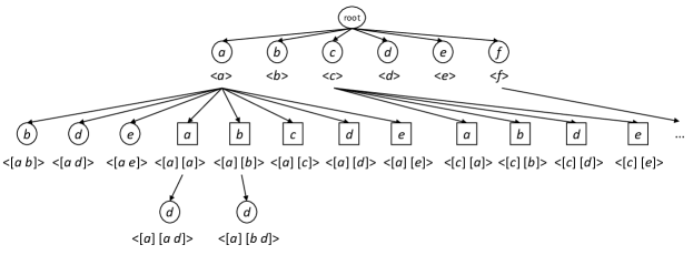
Figure 1. A lexicographic-sequential (LS)-tree (Lin et al., 2017).

For instance, in Fig. 1, $<$a$>$ to $<$f$>$ are the 1-sequences and they are the offsprings of the root. The I-Concatenation sequence is represented as a circle in Fig. 1 and the S-Concatenation sequence is represented as a square. The LS-tree also shows the number of candidates in the search space to discover the set of HUSPs.

In the pattern mining task (Agrawal et al., 1994; Han et al., 2004; Gan et al., 2019b), especially in sequential pattern mining (Pei et al., 2001; Fournier-Viger et al., 2017), there is a huge computational cost if none upper-bound of the patterns is used to prune the search space. To solve this limitation, the utility-array (Gan et al., 2019d) structure is utilized to efficiently calculate the utility and position of the potential patterns. It is used to maintain the necessary information of the patterns in the processed dataset.

Definition 4.1.

(utility-array (Gan et al., 2019d)) In a $q$-sequence database, suppose all the items in a $q$-sequence $s$ have different unique occurred positions as {$p_{1}$, $p_{2}$, $\cdots$, $p_{k}$}, where {$p_{1}$ $<p_{2}$ $<\cdots<p_{k}$}, and the total number of positions ($p_{k}$) is equal to the length of $s$. The utility-array of a $q$-sequence $s$ = $\langle e_{1},e_{2},\cdots,e_{n}\rangle$ consists of a set of arrays, from left to right in $s$, where $e_{n}$ is the $n$-th element in $s$. For an item $i_{j}$ in each position $p_{k}$ in $s$, it represents an array and contains six fields: array${}_{p_{k}}$ = $[$eid, item, u, ru, next_pos, next_eid$]$, in which (1) eid is the element ID of an element containing $i_{j}$; (2) item is the name of item $i_{j}$; (3) $u$ is the actual utility of $i_{j}$ in position $p_{k}$; (4) $ru$ is the remaining utility of $i_{j}$ in position $p_{k}$; (5) next_pos is the next position of $i_{j}$ in $s$; (6) next_eid is the position of the first item in next element (eid+1) after current element (eid). Besides, the utility-array records the first occurred position of each distinct item in a $q$-sequence $s$.

Table 3. The utility-array structure of $S_{3}$ (notation “-” means empty)

. eid item u ru next_pos next_eid array₁ 1 $a$ $12 $84 3 3 array₂ 1 $b$ $10 $72 4 3 array₃ 2 $a$ $8 $64 - 6 array₄ 2 $b$ $15 $49 6 6 array₅ 2 $c$ $3 $46 7 6 array₆ 3 $b$ $20 $26 - 9 array₇ 3 $c$ $15 $11 - 9 array₈ 3 $e$ $8 $3 - 9 array₉ 4 $d$ $3 $0 - -

The utility-array structure of $S_{3}$ from Table 1 can be illustrated as shown in Table 3. For instance, in Table 3, the distinct items of $S_{3}$ are (a), (b), (c), (d), and (e), respectively. The first occurred positions of a), (b), (c), (d), and (e) in $S_{3}$ are 1, 1, 5, 9, and 8, respectively. Consider the item (b) in Table 3, it occurs in position 2 (array₂), 4 (array₄), and 6 (array₆), respectively. In its first occurred position 2 in $S_{3}$, the element ID is 1, the utility of item (b) is $10, and the remaining utility of item (b) is measured as $72, which is the remaining utility. In addition, the next position of an item (b) in $S_{3}$ is 4 (array₄), and the position of the first item in next element ([(a:2) (b:3) (c:1)]) in $S_{3}$ is 3. Thus, the utility-array can store the necessary information (e.g, utility, position, and sequence order), which can be built during the construction of LS-tree.

In the LS-tree, the utility-array of each node/sequence can be directly constructed from the utility-array of its prefix node, without scanning the database again. We adopt the projection mechanism to recursively construct a series of utility-arrays, as well as their extension nodes (aka super-sequences) with the same prefix in the LS-tree. For each node/sequence in the LS-tree, the transactions with the processed node/sequence are then converted into a utility-array, which is attached to the projected utility-array of the processed node. Thus, the utilities and the upper-bounds of the potential HUSPs (or candidates) can be efficiently measured.

4.2. Two Concatenations

In this section, two basic operations, I-Concatenation and S-Concatenation, in the LS-tree are introduced. In the LS-tree, they are used to generate the combinations of the prefix sequences. In other words, the two operations produce the offspring (also called extensions) of the processed nodes.

Definition 4.2.

Let $t$ and $i_{j}$ represent a sequence and an item, respectively. Additionally, let $<$$t\oplus i_{j}$$>$_{I-Concatenation} represent the I-Concatenation of $t$ with $i_{j}$, in which $i_{j}$ is appended to the last element of a sequence $t$. Moreover, let $<$$t\oplus i_{j}$$>$_{S-Concatenation} represent the S-Concatenation of $t$ with $i_{j}$, in which $i_{j}$ is added as a new element/itemset to the last of $t$. Thus, the size of new sequence $<$$t\oplus i_{j}$$>$_{S-Concatenation} increases by one, but the size of new sequence $<$$t\oplus i_{j}$$>$_{I-Concatenation} does not change.

For instance, we generate the new combinations with a sequence $t$ = $<$[$b$], [$c$]$>$ and a new item $(a)$. The results are $<$$t\oplus a$$>$_{I-Concatenation} = $<$[b], [ca]$>$ and $<$$t\oplus a$$>$_{S-Concatenation} = $<$[b], [c], [a]$>$. Obviously, the number of itemsets in $t$ does not change after I-Concatenation. However, the number of itemsets in new sequence generated by S-Concatenation increases by one. Thus, the complete candidates can be easily produced by the two operations in the search space.

As previously described, utility-array (Gan et al., 2019d) is efficient for retrieving the utilities and upper-bounds of the candidate, and the actual HUSPs can be completely discovered. However, a sequence may have multiple matches in a q-sequence, and therefore the sequence may obtain multiple utilities. It is thus necessary to obtain the accurate positions of the matches, which can be used to measure the utilities and the upper-bound values of the processed node (sequence). For convenience, we introduce the concepts for concatenation.

Definition 4.3.

Let t and s represent a sequence and a q-sequence, respectively, and assume that $t\sim s$. The concatenation point of t in s is defined as the position of the final (last) item within each match. The first concatenation point is called the start point.

For instance, in Table 1, we assume that a sequence $t$ = $<$[b], [c]$>$; and it has three matches in $S_{3}$ = $<$[(a:3) (b:2)], [(a:2) (b:3) (c:1)], [(b:4) (c:5) (e:4)], [(d:3)]$>$ such that $<$[b:2], [c:1]$>$, $<$[b:2], [c:5]$>$, and $<$[b:3], [c:5]$>$. Thus, the concatenation positions of $t$ in $S_{3}$ are 5, 7, and 7, respectively. The start point of $<$[b], [c]$>$ in $S_{3}$ is thus set as 5.

Following the definition of I-Concatenation, a new additive item is appended to the last itemset of the processed sequence. Based on I-Concatenation, the candidate items are the items occurring in the same elements/itemsets in which the concatenation points arise. For instance, the candidate items for I-Concatenation of $<$[b:2], [c:1]$>$ are {(a:2), (b:3)}. For the S-Concatenation, the new items are appended to the last of the sequence as the new itemset. For the S-Concatenation operation, the items in the elements/itemsets after the start point are then considered to be the candidate items of each transaction. In the illustrated example, the start point is equal to 5, which appears in the second element in $S_{3}$. Thus, the items after the second element are considered as the candidate items for S-Concatenation, such as {(b:4), (c:5), (e:4), (d:3)} in $S_{3}$. Since multiple matches of a sequence t in a q-sequence can be obtained, the highest utility of the items in the sequence t is then regarded as the utility of t for q-sequence.

In addition, we define the order of sequences in the proposed USPT algorithm and the LS-tree. Given two sequences, $t_{a}$ and $t_{b}$, then $t_{a}\prec t_{b}$, if 1) the length of $t_{a}$ is less than that of $t_{b}$; 2) $t_{a}$ is I-Concatenation from $t$, while $t_{b}$ is S-Concatenation from $t$; and 3) $t_{a}$ and $t_{b}$ are both I-Concatenation or S-Concatenation from t, and the additive item in $t_{a}$ is alphabetically smaller than that in $t_{b}$. This order of sequences is also suitable for $q$-sequences. For example, $<$[a]$>$ $\prec$ $<$[ab]$>$ $\prec$ $<$[a], [a]$>$ $\prec$ $<$[a], [c]$>$. To retrieve the complete set of HUSPs, all candidates of the two operations (concatenations) are enumerated with the lexicographic order in the LS-tree.

4.3. Upper Bounds and Pruning Strategies

Based on the concepts of LS-tree and utility-array, by adopting the depth-first search strategy and two concatenations, the proposed USPT algorithm can successfully identify the complete HUSPs. However, this process may lead to the problem of combinatorial explosion, since a huge number of candidates may be exhaustively explored in the LS-tree. The reason for this is that the downward closure property (Agrawal et al., 1994) (also called Apriori property) cannot be directly applied to HUSPM. Therefore, to solve the problem of combinatorial explosion for mining the HUSPs, a new property is required. Several concepts of sequences and q-sequences are introduced below.

Definition 4.4.

Assume two $q$-sequences such that t and $t^{\prime}$, if $t\subseteq t^{\prime}$ holds, then the extension of $t\in t^{\prime}$ is the suffix of $t^{\prime}$ after $t$. Thus, it can be denoted as $<$$t^{\prime}$-$t$$>_{rest}$. Let t and s represent a sequence and a q-sequence, respectively. If $t\sim s_{k}\wedge s_{k}\subseteq s$ $(t\subseteq s)$ holds, then the superset (extension) of $t$ in $s$ is the rest of $s$ after $s_{k}$, which can be denoted as $<$$s$ - $t$$>_{rest}$, and $s_{k}$ represents the first match of $t$ in $s$.

For instance, two q-sequences such as $s$ = $<$[b:2], [c:5]$>$ and $S_{3}$ are given, where $S_{3}$ is shown in Table 1. The superset of $s$ in $S_{3}$ is $<$$S_{3}$ - $s$$>$_rest = $<$[(e:4)], [(d:3)]$>$. Given a sequence $t$ = $<$[b], [c]$>$, three matches of $t$ in $S_{3}$ are existed, and the first one is $<$[b:2], [c:1]$>$. Thus, $<$$S_{3}$ - $t$$>$_rest = $<$[(b:4) (c:5) (e:4)], [(d:3)]$>$.

Definition 4.5.

The set of extension items of a sequence $t$ in a sequential database is denoted as $I(t)_{rest}$, and defined as:

(1) $$I(t)_{rest}=\{i_{j}|i_{j}\in<s-t>_{rest}\wedge t\subseteq s\wedge s\in QSD\}.$$

Definition 4.6.

The sequence-weighted utilization (SWU) (Yin et al., 2012) of a sequence $t$ in a $QSD$ is denoted as $SWU(t)$, and defined as:

(2) $$SWU(t)=\sum_{s\in QSD}\{u(s)|t\subseteq s\}.$$

From the given example, because $<$$S_{3}$ - $t$$>$_rest = $<$[[(b:4) (c:5) (e:4)], [(d:3)]$>$ in $S_{3}$, I($<$[b], [c]$>$)_rest = {$b,c,e,d$}. In Table 1, $SWU$($<$b$>$) = $u(S_{1})$ + $u(S_{2})$ + $u(S_{3})$ + $u(S_{4})$ + $u(S_{5})$ + $u(S_{6})$= $56 + $67 + $94 + $67 + $76 + $81 = $441, and $SWU$($<$f$>$) = $u(S_{6})$ = $81. Consider $t$ = $<$[b], [c]$>$, SWU($<$[b], [c]$>$) = $u(S_{1})$ + $u(S_{2})$ + $u(S_{3})$ + $u(S_{4})$ + $u(S_{5})$ = $56 + $67 + $94 + $67 + $76 = $360.

Theorem 4.7 (Sequence-Weighted Downward Closure property, SWDC (Yin et al., 2012)).

Given a sequential database $QSD$ and two sequences $t$ and $t^{\prime}$. Based on the concepts of SWU, if $t\subseteq t^{\prime}$ holds, then we can obtain the following property as:

(3) $$SWU(t^{\prime})\leq SWU(t).$$

Theorem 4.8.

Given a sequential database $QSD$ and a sequence $t$, then the following equation holds:

(4) $$u(t)\leq SWU(t).$$

The SWDC property and Theorem 4.8 ensure that if the $SWU$ of a sequence $t$ is no larger than a threshold, then the utility of $t$ and any of its super-sequences are also less than this threshold. Therefore, numerous unpromising candidates can be pruned. To speed up the mining performance, the concept of sequence-weighted utilization (SWU) (Yin et al., 2012) is proposed to maintain the extended downward closure property for mining HUSPs. Thus, the search space can be reduced and some unpromising candidates can be promptly pruned. However, the $SWU$ of a sequence t is usually greater than its actual utility of t. To make the designed algorithm more efficient, the remaining utility model (Yin et al., 2012) is introduced to estimate the lower upper-bound values of the candidates.

Definition 4.9.

Let $SEU(t)$ denote the sequence extension utility of a sequence $t$ in a sequential database $QSD$. As an upper bound, the sequence extension utility (SEU) (Gan et al., 2019d) can be defined as:

(5) $$SEU(t)=\sum_{s\in QSD}\{u(t,s)+u(<s-t>_{rest})|t\subseteq s\}.$$

It should be noted that u($<$s - t$>_{rest}$) is the remaining utility with respect to the first match of $t$ in $s$, which is kept as the fourth field in the utility-array. For instance, in Table 1, suppose a sequence $t$ = $<$[b], [c]$>$, u($<$$S_{2}$ - $t$$>$_rest) = u($<$(d:3), (e:4)$>$, $S_{2})$ = $3 + $8 = $11. Thus, $SEU(t)$ = ($u(t,S_{1})$ + u($<$$S_{1}$ - $t$$>$_rest)) + ($u(t,S_{2})$ + u($<$$S_{2}$ - $t$$>$_rest)) + ($u(t,S_{3})$ + u($<$$S_{3}$ - $t$$>$_rest)) + ($u(t,S_{4})$ + u($<$$S_{4}$ - $t$$>$_rest)) + ($u(t,S_{5})$ + u($<$$S_{5}$ - $t$$>$_rest)) = ($27 + $10) + ($31 + $11) + ($30 + $46) + ($37 + $11) + ($35 + $11) = $249, which is less than SWU($t$)( = $360).

Theorem 4.10.

Suppose two sequences, $t$ and $t^{\prime}$, in QSD. If $t\subseteq t^{\prime}$ holds, then:

(6) $$SEU(t^{\prime})\leq SEU(t).$$

Theorem 4.11.

Given a sequence t in $QSD$, then:

(7) $$u(t)\leq SEU(t).$$

Proof.

$\displaystyle u(t)$ = $\sum_{s\in QSD}\{u(t,s)|t\subseteq s\}\leq\sum_{s\in QSD}\{u(t,s)+u(<s-t>_{rest})|t\subseteq s\}$ = $SEU(t)$. ∎

Theorems 4.10 and 4.11 indicate that for a sequence $t$ in sequence database, if $SEU(t)$ is no greater than a minimum utility threshold, then the utility of $t$ and any of its super-sequences are no greater than this minimum utility threshold. However, the upper bounds (both $SWU$ and $SEU$) cannot be directly utilized in our USPT framework since each item may obtain its individualized minimum utility threshold. Thus, by using the upper bounds of $SWU$ and $SEU$, the USPT framework does not hold the initial downward closure property. For instance, let $t^{\prime}$ be an extension (super-sequence) of $t$; although the $SEU$ or $SWU$ of $t$ is no greater than the minimum utility threshold of $t$, $t^{\prime}$ still has the possibility for becoming a high-utility sequential pattern.

As mentioned, the USPT framework first studies the individualized threshold for each item in utility mining. Thus, several new theorems are presented to hold the downward closure property for correctly and completely mining HUSPs.

Definition 4.12.

The potential minimum utility threshold of a sequence $t$ in QSD is denoted as PMIU$(t)$. Thus, PMIU$(t)$ is the potential least mu threshold among $t$ and its extensions, and defined as:

(8) $$PMIU(t)=min\{mu(i_{j})|i_{j}\in t\vee i_{j}\in I(t)_{rest}\}.$$

Obviously, the concept of PMIU is different from MIU. The reason is that PMIU is related to a sequence $t$ and its extensions, while MIU is only related to a sequence $t$. For instance, in Table 1, PMIU($<$[b], [c]$>$) = min{$mu(i_{j})|i_{j}\in$$<$[b], [c]$>$$\vee i_{j}\in${b, c, e, d}} = min{$500, $500, $200, $500} = $200.

Theorem 4.13.

Based on the definition of HUSP (cf. Definition 3.9), assume a sequence $t$, and let UB$(t)$ be the upper-bound on utility of $t$. We have the theorem as: if $UB(t)<PMIU(t)$, then $t$ and any of its super-sequences will not be the HUSPs.

Proof.

Let $t^{\prime}$ be a extension (super-sequence) of $t$, then $\{i_{j}|i_{j}\in t^{\prime}\}\subseteq\{i_{j}|i_{j}\in t\vee i_{j}\in I(t)_{rest}\}$ and $I(t^{\prime})_{rest}\subseteq I(t)_{rest}$ hold. It is then obtained that $u(t^{\prime})\leq UB(t^{\prime})$ and $u(t)\leq UB(t)$. Next, the following equation can be obtained:

$$u(t^{\prime}) \leq UB(t^{\prime})$$

$$<PMIU(t)=min\{mu(i_{j})|i_{j}\in t\vee i_{j}\in I(t)_{rest}\}$$

$$\leq min\{mu(i_{j})|i_{j}\in t^{\prime}\vee i_{j}\in I(t^{\prime})_{rest}\}=PMIU(t^{\prime})$$

$$\leq min\{mu(i_{j})|i_{j}\in t^{\prime}\}=MIU(t^{\prime}).$$

$$u(t) \leq UB(t)$$

$$<PMIU(t)=min\{mu(i_{j})|i_{j}\in t\vee i_{j}\in I(t)_{rest}\}$$

$$\leq min\{mu(i_{j})|i_{j}\in t\}=MIU(t).$$

It is then ensured that $t$ and $t^{\prime}$ will not be the HUSPs. ∎

Based on Theorem 4.13, if the upper-bound of a sequence $t$ is no greater than the PMIU of $t$, $t$ and any of its super-sequences will not be the HUSPs. The reason for this is that the upper-bound is the maximum utility of a sequence in all possible combinations, which can be either the $SWU$ or $SEU$ of t. In addition, the PMIU is the least and minimum threshold of the sequence. According to the above theorems, the correctness and completeness of the designed USPT algorithm can be guaranteed for mining the HUSPs.

PMIU-based SEU Strategy: The candidate sequences whose SEU values are no greater than their PMIU values are discarded from the candidate set so that their child nodes (or called extensions) are not generated and explored in the LS-tree.

The candidate items for the generation, e.g., I-Concatenation or S-Concatenation of $t$, are measured by their $SWU$ values to reduce the search space. If the $SWU$ value is less than the PMIU value, the candidate item is removed since the super-sequences of $t$ concatenated with this candidate item can not be HUSPs. The set of I-Concatenation or S-Concatenation sequences $t^{\prime}$ ($t^{\prime}$ is the concatenation of $t$ and a candidate item) are determined by their $SEU$ values to check whether they are the candidate sequences. If the $SEU$ of a sequence $t^{\prime}$ is less than its PMIU, then $t^{\prime}$ can be safely discarded since $t^{\prime}$ and any of the super-sequences of $t^{\prime}$ cannot be HUSPs.

The designed baseline USPT algorithm can be used to find the HUSPs correctly and completely. However, the search space of the baseline USPT algorithm is still huge since it utilizes the $SWU$ and $SEU$ over-estimated values, which is much larger than the actual utility of the pattern. Three strategies are developed here to speed up mining performance by promptly pruning the unpromising candidates in the search space. We first utilize a tighter upper-bound on utility for mining HUSPs (Wang et al., 2016), and the details are given below.

Definition 4.14.

The prefix extension utility (PEU) (Wang et al., 2016) of a sequence $t$ in a q-sequence $s$ is defined as PEU$(t,s)$ = $max\{u(s_{k})+u(\textnormal{$<$}s\textnormal{$-$}s_{k}\textnormal{$>$}_{rest})|t\sim s_{k}\wedge s_{k}\subseteq s\}$. Note that here $u(\textnormal{$<$}s\textnormal{$-$}s_{k}\textnormal{$>$}_{rest})$ is the $s_{k}$ match but not the first match of $t$ in $s$.

For example, assume a sequence t = $<$[b], [c]$>$, t has 3 matches in $S_{2}$, which are $<$[b:1], [c:3]$>$, $<$[b:1], [c:2]$>$ and $<$[b:5], [c:2]$>$. It can be obtained that $u$($<$$S_{2}$ - $<$[b:1], [c:3]$>>_{rest}$) = $u$($<$[(e:2)], [(a:1) (c:2) (d:3) (e:4)]$>$) = $25, $u$($<$$S_{2}$ - $<$[b:1], [c:2]$>>_{rest})$ = $u$($<$[(d:3) (e:4)]$>$) = $11, and $u$($<$$S_{2}$ - $<$[b:5], [c:2]$>>_{rest}$) = $u$($<$[(d:3) (e:4)]$>$) = $11. The utilities of 3 matches are $14, $11, and $31, respectively. Thus, PEU($<$[a], [b]$>$, $S_{2}$) = max{$14 + $25, $11 + $11, $31 + $11} = $42. Obviously, the concept of PEU is different from SEU.

Definition 4.15.

The prefix extension utility (PEU) (Wang et al., 2016) of a sequence $t$ in $QSD$ is denoted as PEU$(t)$ and defined as PEU$(t)=\sum_{s\in QSD}\{PEU(t,s)|t\subseteq s\}$. Thus, PEU is the maximal utility of an extension in a sequence or database.

For instance, in Table 1, it is assumed a sequence t = $<$[b], [c]$>$, $PEU(t)$ is measured as $SEU(t,S_{1})$ + $SEU(t,S_{2})$ + $SEU(t,S_{3})$ = $SEU(t,S_{4})$ + $SEU(t,S_{5})$ = $37 + $42 + $59 + $48 + $46 = $232, which is smaller than $SEU$(t) = $249.

Theorem 4.16.

Assume two sequences t and $t^{\prime}$ in QSD. If t $\subseteq$ $t^{\prime}$ holds, then:

(9) $$PEU(t^{\prime})\leq PEU(t).$$

Proof.

Detailed proof can be referred to (Wang et al., 2016). ∎

Thus, Theorem 4.16 shows that if $PEU$ of a sequence $t$ is no greater than a threshold, then the $PEU$ values of its super-sequences are no greater than this threshold. The $PEU$ concept holds the downward closure property.

Theorem 4.17.

Suppose a sequence $t$ in $QSD$, then:

(10) $$u(t)\leq PEU(t).$$

Proof.

Detailed proof can be referred to (Wang et al., 2016). ∎

From Theorems 4.13, 4.16, and 4.17, the completeness and the correctness of the mined HUSPs can be ensured. If the PEU of a sequence $t$ is no greater than the PMIU of $t$, then the utility of $t$ is no greater than the $MIU$ value of t; the utilities of its extensions/super-sequences are no greater than their $MIU$ values ($t$ and the super-sequences of $t$ are not HUSPs).

Theorem 4.18.

Suppose a sequence t in QSD, then:

(11) $$PEU(t)\leq SEU(t)\leq SWU(t).$$

Based on Theorem 4.18, it can be seen that PEU holds a tighter upper-bound value compared to $SEU$ and $SWU$. Thus, the designed algorithm can greatly reduce the unpromising candidates based on the PEU model than that of the $SEU$ and $SWU$ models. The PEU model can be used to estimate the utility values for a candidate sequence and its super-sequences. Therefore, if the PEU of a sequence $t$ is no greater than the PMIU of $t$, then $t$ and any of its super-sequences will not be considered as the HUSPs.

PMIU-based PEU Strategy: The candidate sequences whose PEU values are no greater than their PMIU values are discarded from the candidate set so that their child nodes (or called extensions) are not generated and explored in the LS-tree.

A huge number of candidates are generated using I-Concatenation and S-Concatenation for a processed sequence t. Based on the PMIU concept in the addressed problem, we further propose the PMIU-based pruning strategy (PUK), which can also be used to reduce the search space by promptly removing unpromising candidates.

Theorem 4.19.

For a sequence $t$ in $QSD$, assume an item $i_{j}$ is an I-Concatenation or S-Concatenation candidate item of $t$. Two situations can be considered to produce the super-sequences/extensions as follows:

Case 1: the maximal utility of $<$$t\oplus i_{j}$$>$_{I-Concatenation} is always less than or equal to the upper bound on utility (e.g., SEU, PEU) of $t$;

Case 2: the maximal utility of $<$$t$$\oplus i_{j}$$>$_{S-Concatenation} is always less than or equal to the upper bound on utility (e.g., SEU, PEU) of $t$.

Proof.

For Case 1, let $t^{\prime}$ = $<$$t\oplus i_{j}$$>$_{I-Concatenation}. Since $PEU(t^{\prime})$ = $\sum_{s\in QSD}\{PEU(t^{\prime},s)|t^{\prime}\subseteq s\}$ and $PEU(t^{\prime},s)\leq PEU(t,s)$. For convenience, as proven in Theorem 4.16, $PEU(t^{\prime})\leq PEU(t)$. According to Theorem 4.17, $u(t^{\prime})\leq PEU(t^{\prime})$ holds. Thus, $u(t^{\prime})\leq PEU(t^{\prime})=\sum_{s\in QSD}\{PEU(t^{\prime},s)|t^{\prime}\subseteq s\}\leq\sum_{s\in QSD}\{PEU(t,s)|t\subseteq s\}$, we have $u(t^{\prime})\leq PEU(t)$. Case 2 can be verified in the same way. ∎

Based on the PMIU-based SEU strategy and PEU strategy, we further propose the general strategy to prune the unpromising $k$-sequences during spanning the LS-tree.

PMIU-based pruning unpromising $k$-sequences strategy (PUK strategy): Assume a sequence $t$ in $QSD$, then two situations can be considered as follows:

Case 1: if $i_{j}$ is a I-Concatenation candidate item for $t$ and the upper bound on utility (e.g., SEU, PEU) of $t$ is no greater than PMIU($<$$t\oplus i_{j}$$>$${}_{I-Concatenation})$, then $i_{j}$ can be removed from the set of candidate items for I-Concatenation of $t$;

Case 2: if $i_{j}$ is a S-Concatenation candidate item for $t$ and the upper bound on utility (e.g., SEU, PEU) of $t$ is no greater than PMIU($<$$t\oplus i_{j}$$>$${}_{S-Concatenation})$, then $i_{j}$ can be removed from the set of candidate items for S-Concatenation of $t$.

The PMIU-based PUK strategy is used to promptly prune unpromising candidates for the I-Concatenation and S-Concatenation of $t$ without evaluating the PEU values for $<$$t\oplus i_{j}$$>$_{I-Concatenation} and $<$$t$ $\oplus i_{j}$$>$_{S-Concatenation}, where $t$ is a sequence in a dataset. The reason for this is that the upper-bound value can be easily evaluated from the utility-arrays of $t$. Thus, the designed algorithm can reduce the computational cost with a small set of candidates for either I-Concatenation or S-Concatenation of $t$.

It is important to notice that PEU provides a tighter upper-bound than SEU, thus the search space for mining the HUSPs can be greatly reduce. In addition, more unpromising candidates can be reduced in the search space with the developed PMIU-based pruning strategies. For example, the candidates for I-Concatenation or S-Concatenation of the processed sequence $t$ can be pruned by SEU and PUK strategy and the utility-arrays of $t$ will be re-calculated. After that, the candidates for I-Concatenation and S-Concatenation of the processed $t$ will be measured by PUK strategy instead of their $SWU$ values.

4.4. The Designed USPT Algorithm

Based on the above properties of upper bounds on utility and utility-array, the main procedures of the designed USPT algorithm are introduced in Algorithm 1 and Algorithm 2. Algorithm 1 shows that the whole process of USPT has three input parameters as follows: 1) QSD; 2) utable; and 3) M-table. The USPT algorithm first scans $QSD$ once to construct utility-array of each $s\in QSD$, denoted the set as $D.ua$ (Line 1). After that, USPT processes each 1-sequence $i_{j}\in QSD$ one-by-one with the lexicographic order. Based on the constructed $D.ua$, it first constructs the projected utility-array $(D.ua)|_{<i_{j}>}$ of $i_{j}\in QSD$ to store the information (e.g., utility, position, and sequence order) (Line 4). Then the actual overall utility, $SWU$, PMIU, and $MIU$ of each 1-sequence are respectively calculated from the projected $(D.ua)|_{<i_{j}>}$ (Line 5). USPT also updates the remaining utilities in $D.ua$ by removing the unpromising items $SWU$($<$$i_{j}$$>$) $<$ PMIU($<$$i_{j}$$>$) from $D.ua$ (Line 6, adopts the SWU strategy). For each processed 1-sequence, it is discovered as a candidate item if its $SWU$ value is no less than the PMIU value (Lines 7 to 12). If the utility of a 1-sequence is no less than the MIU value, then this 1-sequence is outputted as a HUSP (Lines 8-10). After that, the candidate pattern that meets the condition as $SWU$($<$$i_{j}$$>$) $\geq$ PMIU($<$$i_{j}$$>$) has become the prefix of Span-Search function for mining prefix-based HUSPs (Line 11).

Input: QSD, a sequential database with quantitative values; utable, a table with the unit utility of each item; M-table, a table with the threshold of each item.

Output: The set of HUSPs.

1

2initialize $D.ua$ = $\emptyset$, HUSPs $\leftarrow\varnothing$;

3 scan $QSD$ once to construct utility-array of each $s\in QSD$, denoted the set as $D.ua$;

4

5for each 1-sequence $i_{j}\in QSD$ do

6       construct utility-array of $<$$i_{j}$$>$ as $(D.ua)|_{<i_{j}>}$ based on $D.ua$;

7       calculate $SWU$($<$$i_{j}$$>$), $u$($<$$i_{j}$$>$), PMIU($<$$i_{j}$$>$), and $MIU$($<$$i_{j}$$>$);

8       update the remaining utilities in $D.ua$ by removing the unpromising items (the SWU strategy);

9      

10      if $SWU$($<$$i_{j}$$>$) $\geq$ PMIU($<$$i_{j}$$>$) (the SWU strategy) then

11             if $u$($<$$i_{j}$$>$) $\geq$ $MIU$($<$$i_{j}$$>$) then

12                   put $<$$i_{j}$$>$ into HUSPs;

13                  

14             end if

15            call Span-Search($<$$i_{j}$$>$, $(D.ua)|_{<i_{j}>}$);

16            

17       end if

18      

19 end for

return HUSPs

ALGORITHM 1 USPT

As presented at Algorithm 2, the Span-Search procedure utilizes a depth-first search to span all possible sequences with the lexicographic order. The enumerated sequences are produced by two concatenations: I-Concatenation and S-Concatenation, respectively. This function first scans the projected $(D.ua)|_{t}$ once to obtain iItem (the set of candidate items for I-Concatenation) and sItem (the set of candidate items for S-Concatenation) (Lines 1-4). At the same time, the $PEU$ values of the candidate items are calculated from $(D.ua)|_{t}$ (Line 5). Then, this procedure removes the unpromising items from two candidate sets (iItem and sItem) that avoid generating the unpromising I-Concatenation and S-Concatenation for the prefix sequence $t$ (Lines 6-7). Based on Theorems 4.7 and 4.8, these unpromising candidate item $i_{j}$ can be safely discarded. After that, each candidate in the updated sets of iItem and sItem is determined one-by-one.

Details of the Span-Search operation are given below (Lines 8-18). For each item $i\in iItem$, USPT generates a new sequence $t^{\prime}\leftarrow$ $I$-Concatenation$(t,i)$, and constructs the projected utility-array $(D.ua)|_{t^{\prime}}$ based on $(D.ua)|_{t}$ (Lines 9-10). Note that $(D.ua)|_{t}$ is the utility-array of the prefix $t$, thus USPT can easily construct the new projected utility-array for extension node/sequence in LS-tree. The $PEU$, PMIU, utility, and $MIU$ of new sequence $t^{\prime}$ are then calculated from $(D.ua)|_{t^{\prime}}$ (Line 11). If the utility of $t^{\prime}$ is no less than the $MIU$ of $t^{\prime}$, then $t^{\prime}$ is identified as a HUSP (Lines 13-15). If the $PEU$ of $t^{\prime}$ is no less than the PMIU of $t^{\prime}$, then the Span-Search procedure is performed to discover HUSPs which are based on the prefix sequence $t^{\prime}$ (Line 16). The Span-Search procedure is recursively called and terminated if no candidates are generated. For each item $i\in sItem$, it is processed in the same way (Lines 19-29). Finally, the Span-Search procedure returns the set of discovered HUSPs w.r.t. prefix $t$. At the end, the final complete set of HUSPs would be discovered by the designed USPT algorithm.

Input: t: a sequence as prefix; $(D.ua)|_{t}$: the projected utility-array of $t$.

Output: HUSPs: the set of high-utility sequential patterns with prefix $t$.

1

2initialize $iItem$ = $\emptyset$ and $sItem$ = $\emptyset$;

3 scan the projected utility-array $(D.ua)|_{t}$ once to:

4 1) put $I$-Concatenation items of $t$ into iItem;

5 2) put $S$-Concatenation items of $t$ into sItem;

6 3) calculate the PEU values of these items form $(D.ua)|_{t}$;

7

8remove unpromising items $i_{j}\in iItem$ that have PEU$(i_{j})<PMIU(t)$ (the PUK strategy);

9 remove unpromising items $i_{j}\in sItem$ that have PEU$(i_{j})<PMIU(t)$ (the PUK strategy);

10

11for each item $i\in iItem$ do

12       generate new sequence $t^{\prime}\leftarrow$ $I$-Concatenation$(t,i)$;

13       construct the projected utility-array $(D.ua)|_{t^{\prime}}$ based on $(D.ua)|_{t}$;

14       determine $u$($t^{\prime}$), $PEU$($t^{\prime}$), PMIU($t^{\prime}$), and $MIU$($t^{\prime}$);

15      

16      if  PEU$(t^{\prime})\geq PMIU(t^{\prime})$ (the PUK strategy) then

17            

18            if $u(t^{\prime})\geq MIU(t^{\prime})$ then

19                   output $t^{\prime}$ into HUSPs;

20                  

21             end if

22            call Span-Search$(t^{\prime},(D.ua)|_{t^{\prime}})$;

23            

24       end if

25      

26 end for

27

28for each item $i\in sItem$ do

29       generate new sequence $t^{\prime}\leftarrow$ $S$-Concatenation$(t,i)$;

30       construct the projected utility-array $(D.ua)|_{t^{\prime}}$;

31      

32      determine $u$($t^{\prime}$), $PEU$($t^{\prime}$), PMIU($t^{\prime}$), and $MIU$($t^{\prime}$);

33      

34      if  PEU$(t^{\prime})\geq PMIU(t^{\prime})$ (the PUK strategy) then

35            

36            if $u(t^{\prime})\geq MIU(t^{\prime})$ then

37                   output $t^{\prime}$ into HUSPs;

38                  

39             end if

40            call Span-Search$(t^{\prime},(D.ua)|_{t^{\prime}})$;

41            

42       end if

43      

44 end for

45

46return HUSPs

ALGORITHM 2 Span-Search

5. An Example of the Proposed Algorithm

In this section, a running example is given to describe the designed USPT and its variations step-by-step. Assume that the individualized minimum utility thresholds of all items in Tables 1 and 2 are respectively assigned in an M-table, as follows: M-table = {$mu(a)$, $mu(b)$, $mu(c)$, $mu(d)$, $mu(e)$, $mu(f)$} = {$500, $500, $500, $500, $200, $70}. Note that these values can be adjusted based on the user’s preference and prior knowledge.

To remove the unpromising items from the database, the USPT method first evaluates the $SWU$ value of each item $i_{j}$ in QSD against $min\{mu(i_{j})|i_{j}\in QSD\}$. The unsatisfied items are then removed from QSD and the size of QSD can be refined. After that, the USPT algorithm scans the refined database once to calculate the transaction utility, and the results are $\{$$u(S_{1})$: $56, $u(S_{2})$: $67, $u(S_{3})$: $94, $u(S_{4})$: $67, $u(S_{5})$: $76, $u(S_{6})$: $81$\}$. The algorithm also generates the utility-arrays for each transaction in QSD. The projected database for each 1-sequence is built based on these utility-arrays. The $SWU$, PMIU, $MIU$, and actual utility of each 1-sequence are calculated from the projected database, respectively. The obtained results are shown in Table 4.

Table 4. The obtained information of 1-sequences in $QSD$.

1-sequence	a	b	c	d	e	f
SWU($<$$i_{j}$$>$)	$360	$441	$441	$360	$441	$81
PMIU($<$$i_{j}$$>$)	$200	$200	$200	$200	$200	$70
u($<$$i_{j}$$>$)	$48	$130	$72	$17	$48	$24
MIU($<$$i_{j}$$>$)	$500	$500	$500	$500	$200	$70

In this example, the 1-sequence $<$a$>$ is first processed with the lexicographic order. Since $SWU$($<$a$>$) ¿ PMIU($<$a$>$) but $u$($<$a$>$) $<$ $MIU$($<$a$>$), $<$a$>$ is not a HUSP, but the super-sequences of $<$a$>$ should be explored. Thus, $<$a$>$ becomes the prefix pattern for the later mining processes. The designed Span-Search function is then performed on $<$a$>$ to generate its super-sequences. USPT scans the projected utility-array $(D.ua)|_{a}$ once to: 1) put $I$-Concatenation items of $t$ into iItem; 2) put $S$-Concatenation items of $t$ into sItem; and 3) calculate the PEU values of these items form $(D.ua)|_{a}$. For 1-sequence $<$a$>$, the candidates are updated as iItem = {$b,c,d,e$} for $I$-Concatenation of $<$a$>$, and sItem = {$a,b,c,d,e$} for $S$-Concatenation of $<$a$>$. In this example, the candidate item $\{a\}$, appearing in $S_{3}$ and $S_{5}$, is different from the prefix $<$a$>$, and it can be used for the S-Concatenation of $<$a$>$. The PEU values of the candidate items are respectively calculated as {PEU($a$): $312, PEU($b$): $359, PEU($c$): $218, PEU($d$): $156, PEU($e$): $104, PEU($f$): $81}, and those unpromising items $d$, $e$, and $f$ are removed from the sets of iItem and sItem since their PEU values are less than PMIU($<$a$>$) (= 200). Thus, only iItem = {$a,b,c$} and sItem = {$a,b,c$} are used to span the LS-tree with I-Concatenation and S-Concatenation, respectively.

After that, the USPT framework first generates new sequence $t^{\prime}$ = $<$a, a$>$ and constructs the projected utility-array $(D.ua)|_{t^{\prime}}$. However, this $(D.ua)|_{t^{\prime}}$ is empty since $<$a, a$>$ does not occurred in Table 1. For the next new sequence $<$a, b$>$, its projected utility-array is then constructed. This utility-array is not empty and the utility values of $<$a, b$>$ for the I-Concatenation of $<$a$>$ are {u($<$a, b$>$): $55, PEU($<$a, b$>$): $170, PMIU($<$a, b$>$): $500, MIU($<$a, b$>$): $500}. Based on the PEU-based PUK strategy, the candidate sequence $<$a, b$>$ and its super-sequences could not be the HUSPs. Therefore, USPT stops calling the Span-Search function and continues to determinate the new candidate sequence $<$a, c$>$.

After checking all candidates for I-Concatenation with prefix $<$$a$$>$, the USPT algorithm begins the similar projection-based search for S-Concatenation with prefix $<$$a$$>$. Three sequences $<$[$a$], [$a$]$>$, $<$[$a$], [$b$]$>$, and $<$[$a$], [$c$]$>$, are then performed to calculate their PEU, PMIU, utility, and $MIU$ values by constructing the projected utility-array $(D.ua)|_{t^{\prime}}$, based on $(D.ua)|_{a}$. After that, the Span-Search approach is continuously performed on next 1-sequence $<$$b$$>$ to discover HUSPs, using the similar operations on 1-sequence $<$$a$$>$. This procedure is then processed repeatedly until no candidates are generated. In this illustrated example, the final discovered HUSPs are shown in Table 5.

Table 5. The discovered HUSPs.

$HUSP$	$utility$	PMIU
$<$[b], [c, e]$>$	$200	$200
$<$[f], [b, c], [b]$>$	$73	$70
$<$[f], [b, c], [b, e]$>$	$81	$70
$<$[f], [b], [b, e]$>$	$72	$70

From Table 5, if the user focuses on the items (f) and (e), then the mu values for (e) and (f) can be set lower. Even though the utilities of these sequences are not high, the designed algorithm can identify the sequences containing interesting items.

6. Experimental Results

Several experiments were performed to evaluate the efficiency and effectiveness of the designed USPT framework. The compared algorithms include the baseline algorithm and its variations with several developed pruning strategies. For convenience, the baseline is called USPT1 (without Line 6 in Algorithm 1 and Lines 6-7 in Algorithm 2), the variation without Lines 6-7 in Algorithm 2 is called USPT2, and the variation with all three pruning strategies as shown in Algorithm 2 is called USPT. This is the first work to handle the issue of discovering the HUSPs with individualized thresholds. Therefore, the baseline algorithm with its variations are compared to evaluate the mining efficiency, in terms of execution time, pattern analysis, memory consumption, and scalability test.

Besides, it is important to notice that the addressed USPT framework equals to high-utility sequential pattern mining (HUSPM) whereas all the individualized thresholds in M-table equal to the unified minimum utility threshold. Therefore, a well-known HUS-Span (Wang et al., 2016) algorithm is compared with USPT to evaluate their effectiveness. A model introduced in (Lin et al., 2016b) was used to set the varied thresholds for the items in datasets. The function of our model was set as: $mu(i_{j})=max\{\beta\times u(i_{j}),LMU\}$. In this function, $LMU$ represents the least minimum utility threshold, which can be adjusted by user’s preference; $u(i_{j})$ shows the utility of each item $i_{j}$ in the dataset; and $\beta$ states the constant factor, which is for adjusting the $mu$ value of items.

6.1. Experimental Environment and Datasets

The all compared algorithms were implemented in Java language, and the experiments were conducted on a PC ThinkPad T470p. An Intel(R) Core(TM) i7-7700HQ CPU was used with 32 GB of main memory. The running operating system was set as 64-bit Microsoft Windows 10.

In the experiments, one synthetic dataset (Agrawal and Srikant, 1994) and five real-life datasets were used to evaluate the performance of the designed USPT algorithm. The characteristics of these datasets are described in Table 6 and Table 7, and details are as follows:

Table 6. Parameters of used datasets.

$\mathbf{\#|D|}$	Number of sequences
$\mathbf{\#|I|}$	Number of distinct items
#S	Length of a sequence $s$
#Seq	Number of elements per sequence
#Ele	Average number of items w.r.t. per element/itemset

Table 7. Dataset features

Dataset	#$|D|$	#$|I|$	avg(#S)	max(#S)	avg(#Seq)	ave(#Ele)
Sign	730	267	52	94	51.99	1.0
Bible	36,369	13,905	21.64	100	17.85	1.0
SynDataset-160k	159,501	7,609	6.19	20	26.64	4.32
Leviathan	5,834	9,025	33.81	100	26.34	1.0
MSNBC	31,790	17	13.1	100	5.33	1.0
yoochoose-buys	234,300	16,004	1.13	21	2.11	1.97

• Sign: a real-life sign language utterance dataset, which was created by the National Center for Sign Language and Gesture Resources at Boston University. It has 730 sequences with total 267 distinct items. Each utterance in this dataset is associated with a segment of video with a detailed transcription.

• Bible: a real-life dataset of the conversion of the Bible into a set of sequences and each word is an item.

• C8S6T4I3D$|$X$|$K: a synthetic sequential dataset, which was generated by IBM Quest Dataset Generator (Agrawal and Srikant, 1994), and used to evaluate the scalability of USPT. Note that SynDataset-160K is a subset of C8S6T4I3D$|$X$|$K, and only contains 160,000 sequences.

• Leviathan: a conversion of the 1651 novel, Leviathan, by Thomas Hobbes. Each word is an item in the sequences.

• MSNBC: a real-life click-stream dataset, which was accessed from the UCI repository, and all the shortest sequences are removed. It contains 31,790 sequences and 17 distinct items.

• yoochoose-buys: a real-life e-commercial dataset, which was collected from YOOCHOOSE GmbH. We preprocess this dataset by removing some noise data.

Since these sequence datasets except for yoochoose-buys do not contain the utility values, a well-known simulation model (Liu et al., 2005) was utilized to generate the internal and external utility values of the items in these datasets. For the quantity value of each item, a random function was used to generate its value in a range from 1 to 5. A log-normal distribution was used to randomly assign the unit utility value of the items in a range from 1 to 1000. All the test datasets, except for C8S6T4I3D$|$X$|$K, can be accessed from the SPMF website.

6.2. Runtime Analysis

In our experiments, each runtime of the designed approach with different pruning strategies was first evaluated to analyze the efficiency of USPT algorithm. Results under various LMUs with a fixed $\beta$ of runtime comparison are shown in Fig. 2. Moreover, results under various $\beta$ with a fixed LMU are shown in Fig. 3.

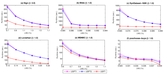
Figure 2. Runtime under various LMU with a fixed $\beta$.

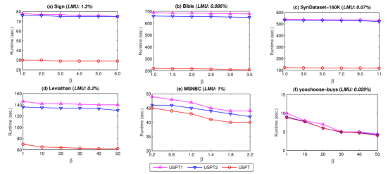
Figure 3. Runtime under various $\beta$ with a fixed LMU.

As shown in Figs. 2 and 3, the hybrid USPT which utilizes all pruning strategies outperformed the basic USPT1 and USPT2 on all the datasets. The runtime always shows that USPT $<$ USPT2 $<$ USPT1. Specifically, USPT was up to one or more orders of magnitude faster than the baseline algorithm without any improvements. For example, when varying LMU from 0.065% to 0.090% on the SynDataset-160K dataset, as shown in Fig. 2(c), the runtime of USPT changed from 130 seconds to 110 seconds, while the consumed runtime of USPT1 changed from 850 seconds to 220 seconds. The same trend can also be observed in Figs. 2(a) to 2(f), and also in Figs. 3(a) to 3(f). The reason for this is that USPT utilizes a tighter upper-bound on sequence utility (e.g., PEU) to prune the unpromising candidates earlier; it is more powerful than the sequence-weighted utilization (SWU) that was used in the basic USPT1 algorithm. Therefore, the proposed three pruning strategies are shown to be effective and efficient to speed up mining performance.

As shown in Fig. 2, the runtime for all the implemented algorithms increased along with a decrease of the LMU on all conducted datasets. When the LMU was set lower, the runtime of USPT remained stable, but the runtime of the baseline USPT1 and USPT2 algorithms dramatically increased. This is reasonable since a large number of candidates are needed and generated with a loose upper-bounds utility, which can be seen in Figs. 2(a), 2(b), and 2(c).

Moreover, it is interesting to notice that the runtime of the compared approaches always decreased with the increase of $\beta$, which is shown in Figs. 3(a) to 3(f). This is because the constant factor $\beta$ increases the $mu$ values of items. The least minimum utility thresholds of the desired sequential patterns would also be increased. Thus, less runtime was required to find fewer candidates for mining HUSPs. The developed UPST algorithm could discover the final results within a reasonable time, and the enhanced variants could achieve good performance in terms of runtime.

6.3. Pattern Analysis

With the same parameter settings as in Section 6.2, the size of the derived candidates and the final set of HUSPs were evaluated. The goal was to analyze the effectiveness of the proposed USPT algorithm and the effect of three pruning strategies. Note that #Candidate 1, #Candidate 2, and #Candidate 3 respectively showed the size of candidates generated by the USPT1, USPT2, and USP algorithms, and # HUSPs denoted the number of the final discovered HUSPs. The pattern results with a fixed $\beta$ and various LMUs and with a fixed LMU and various $\beta$ are illustrated in Tables 8 and 9, respectively.

Table 8. Number of patterns under a fixed $\beta$ with various LMU.

		Fixed $\beta$ with various LMU
		LMU1	LMU2	LMU3	LMU4	LMU5	LMU6
	#Candidate 1	30,968,191	15,039,951	8,494,306	5,265,822	3,490,865	2,418,798
($a$) Sign	#Candidate 2	30,931,811	14,969,330	8,433,278	5,230,673	3,453,759	2,417,460
($\beta$: 3.0)	#Candidate 3	4,431,028	2,122,378	1,179,664	722,378	475,204	330,575
	#HUSPs	84,529	59,062	34,479	24,481	17,352	10,970
	#Candidate 1	1,128,248,314	108,332,778	14,062,212	7,764,230	6,997,687	6,548,176
($b$) Bible	#Candidate 2	999,021,192	91,339,687	12,677,343	7,503,766	6,806,316	6,368,189
($\beta$: 1.0)	#Candidate 3	1,260,949	1,042,111	980,736	927,481	878,041	832,596
	#HUSPs	6,001	5,809	5,593	5,345	5,108	4,940
	#Candidate 1	8,752,612	5,357,804	3,313,643	2,122,959	1,394,948	948,352
($c$) Scalability-160K	#Candidate 2	8,736,281	5,347,225	3,307,685	2,117,095	1,389,002	944,719
($\beta$: 1.0)	#Candidate 3	252,361	109,026	50,308	29,337	21,711	17,516
	#HUSPs	58,519	17,741	4,659	1,220	289	90
	#Candidate 1	16,653,274	10,697,194	7,626,524	5,643,813	4,338,173	3,421,703
($d$) Leviathan	#Candidate 2	16,042,628	10,266,172	7,295,498	5,413,709	4,149,152	3,274,113
($\beta$: 1.0)	#Candidate 3	3,000,848	2,025,511	1,447,670	1,078,496	829,904	654,957
	#HUSPs	384,681	238,670	157,953	109,295	80,857	61,440
	#Candidate 1	2,321,973	1,131,628	625,801	385,761	247,973	167,433
($e$) MSNBC	#Candidate 2	2,321,973	1,131,628	625,801	385,761	247,973	167,433
($\beta$: 1.0)	#Candidate 3	951,843	471,188	269,812	171,706	110,153	75,437
	#HUSPs	136	136	136	136	122	113
	#Candidate 1	268,788	226,033	179,922	134,105	88,400	42,266
($f$) yoochoose-buys	#Candidate 2	268,776	226,018	179,905	134,093	88,395	42,255
($\beta$: 1.0)	#Candidate 3	268,408	225,692	179,611	133,832	88,152	42,048
	#HUSPs	258,886	214,309	168,215	122,706	76,789	31,142

Table 9. Number of patterns under a fixed LMU with various $\beta$.

		Fixed LMU with various $\beta$
		$\beta_{1}$	$\beta_{2}$	$\beta_{3}$	$\beta_{4}$	$\beta_{5}$	$\beta_{6}$
	#Candidate 1	5,265,822	5,265,822	5,265,822	5,265,822	5,265,822	5,265,795
($a$) Sign	#Candidate 2	5,230,673	5,230,673	5,230,673	5,230,673	5,230,673	5,230,646
(LMU: 1.3%)	#Candidate 3	722,378	722,378	722,378	722,378	722,378	722,376
	#HUSPs	55,883	45,733	24,481	9,561	4,733	1,517
	#Candidate 1	108,332,778	108,332,778	108,332,778	108,329,765	108,329,702	108,329,702
($b$) Bible	#Candidate 2	91,339,687	91,339,687	91,339,687	91,336,966	91,336,906	91,336,906
(LMU: 0.086%)	#Candidate 3	1,042,111	1,042,111	1,042,111	1,042,111	1,042,111	1,042,111
	#HUSPs	5,809	1,413	503	283	167	88
	#Candidate 1	5,357,804	5,357,804	5,357,804	5,357,804	5,357,804	5,357,804
($c$) Scalability-160K	#Candidate 2	5,347,225	5,347,225	5,347,225	5,347,225	5,347,225	5,347,225
(LMU: 0.07%)	#Candidate 3	109,026	109,026	109,026	109,026	109,026	109,026
	#HUSPs	17,741	17,513	16,737	8,982	352	261
	#Candidate 1	4,338,173	4,338,112	4,337,591	4,332,859	4,290,103	4,093,436
($d$) Leviathan	#Candidate 2	4,149,152	4,149,096	4,148,651	4,144,219	4,104,213	3,919,454
(LMU: 0.2%)	#Candidate 3	829,904	829,873	829,749	829,269	826,212	811,885
	#HUSPs	80,857	78,006	71,399	19,048	8,329	2,052
	#Candidate 1	248,017	248,017	247,973	234,225	231,471	230,921
($e$) MSNBC	#Candidate 2	248,017	248,017	247,973	234,225	231,471	230,921
(LMU: 1%)	#Candidate 3	110,156	110,156	110,153	102,942	101,690	101,582
	#HUSPs	7,539	1,005	122	32	7	2
	#Candidate 1	268,788	266,582	266,011	253,744	102,749	404
($f$) yoochoose-buys	#Candidate 2	268,776	266,573	266,005	253,743	102,747	402
(LMU: 0.029%)	#Candidate 3	268,408	266,372	265,919	253,680	102,709	364
	#HUSPs	258,886	255,471	255,471	230,207	87,290	0

As shown in Tables 8 and 9, the size of the candidates generated by USPT is much fewer that of USPT1 and USPT2. For instance, in the Leviathan dataset, shown in Table 8(d), when $\beta$ was set as 1.0 and LMU was set as 0.20%, the results respectively were #Candidate 1: 3,421,703, #Candidate 2: 3,274,113, and #Candidate 3: 654,957. Among these, only #Candidate 3 was close to the final results of the HUSPs since #HUSPs: 61,440. Therefore, the developed strategies could be used to greatly reduce the size of candidates in the search space for mining the actual HUSPs. The runtime for mining the HUSPs could also be improved. More specifically, the results of the size of candidates imply that the more powerful filtering ability of the enhanced USPT algorithm pruned the unpromising patterns. The runtime in Figs. 2 and 3 show that the developed strategies could improve mining performance because the size of the candidates was reduced in the search space. To obtain the tight upper-bound values of the candidates, USPT1 and USPT2 need to recalculate the remaining utilities in the utility-array structure, which requires the additional computations.

From the above results, it can be observed that with the decrease of the LMU and $\beta$, the number of candidates increases for the USPT, USPT1, and USPT2. However, with the effect of the pruning strategies, USPT and USPT2 have better performances than the baseline USPT1. Therefore, USPT produced much fewer candidates than USPT1 when a lower LMU or $\beta$ was set. It can also be observed that the size of the candidates sharply decreases in Tables 8(b) and 8(e), which is very interesting and reassuring.

6.4. Memory Consumption

The maximal memory consumption of the compared approaches was further evaluated in this subsection. Note that the maximal memory consumption was checked using Java API. Results under various LMUs with a fixed $\beta$ of memory consumption are shown in Fig. 4. Moreover, results of memory consumption under various $\beta$ with a fixed LMU are shown in Fig. 5.

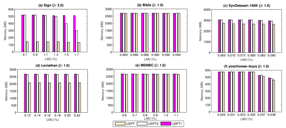
Figure 4. Memory consumption under various LMU with a fixed $\beta$.

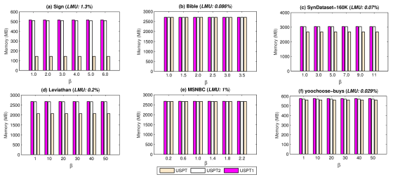
Figure 5. Memory consumption under various $\beta$ with a fixed LMU.

Obviously, three variants of the proposed USPT algorithm consume the stable memory to discover HUSPs with individualized minimum utility thresholds. Among them, USPT1 and USPT2 always consume the similar maximal memory in different parameter settings on all datasets. And the hybrid USPT variant always consumes the least memory on all datasets, and sometimes the gap of memory consumption between USPT and other baselines is large, as shown in Sign (Fig. 4(a) and Fig. 5(a)) and Leviathan (Fig. 4(d) and Fig. 5(d)). According the above experimental results of runtime, the number of generated candidates and memory consumption, we can summarize the conclusion as follows: the designed USPT framework can successfully discover the set of high-utility sequential patterns with individualized thresholds, and the pruning strategies can further be utilized to speedup mining efficiency, in terms of execution time, powerful of pruning unpromising candidates, and the memory consumption.

6.5. USPT Framework vs. Basic HUSPM Model

As mentioned before, a traditional HUSPM algorithm could be a special case of the USPT problem statement whereas the minimum individualized thresholds equal to the unified threshold in HUSPM. In other words, when $\beta$ in the function $mu(i_{j})=max\{\beta\times u(i_{j}),LMU\}$ is set to 0, then the mu value of each item/sequence is equal to LMU. Thus, the basic HUSPM model has become a special case of the USPT problem statement when $\beta$ = 0. In this subsection, a performance comparison of USPT and a traditional HUSPM algorithm was provided. We selected HUS-Span (Wang et al., 2016) as the compared HUSPM algorithm. With the same parameter settings as in Section 6.2, detailed results are presented in Table 10(a) to 10(f), respectively. Note that $\beta$ is set to 0 in USPT, and the LMU equals the unified minimum utility threshold in HUS-Span.

Table 10. Number of patterns under a fixed $\beta$ with various LMU.

		Fixed $\beta$ with various LMU
		LMU1	LMU2	LMU3	LMU4	LMU5	LMU6
	Time*	643	416	278	206	157	119
	Memory*	2,063	2,067	2,067	2,064	2,062	2,064
	#Candidate*	30,971,048	15,039,955	8,494,312	5,265,825	3,490,869	2,418,799
($a$) Sign	#HUSPs*	621,291	245,689	112,001	56,395	30,440	17,274
($\beta$: 3.0)	Time	115	69	46	33	23	19
	Memory	144	144	144	133	133	133
	#Candidate	4,431,158	2,122,378	1,179,664	722,378	475,204	330,575
	#HUSPs	621,291	245,689	112,001	56,395	30,440	17,274
	Time*	-	1,680	1,172	1,088	1,048	1,030
	Memory*	-	3,064	2,966	3,055	2,987	2,900
	#Candidate*	-	108,260,940	14,012,881	7,659,519	6,916,037	6,471,482
($b$) Bible	#HUSPs*	324,599	305,126	287,227	270,850	255,662	241,882
($\beta$: 1.0)	Time	213	210	198	192	189	208
	Memory	2,708	2,708	2,707	2,707	2,705	2,705
	#Candidate	1,260,949	1,042,111	980,736	927,481	878,041	832,596
	#HUSPs	324,599	305,126	287,227	270,850	255,662	241,882
	Time*	2,824	2,022	1,460	1,152	950	820
	Memory*	2,021	1,830	1,734	1,716	1,700	1,512
	#Candidate*	8,752,654	5,357,847	3,313,681	2,123,007	1,394,913	948,397
($c$) SynDataset-160K	#HUSPs*	58,710	17,903	4,794	1,344	394 172
($\beta$: 1.0)	Time	130	119	114	112	109	108
	Memory	2,734	2,679	2,667	2,665	2,665	2,663
	#Candidate	252,361	109,026	50,308	29,337	21,711	17,516
	#HUSPs	58,710	17,903	4,794	1,344	394 172
	Time*	647	474	435	351	289	263
	Memory*	2,720	2,671	2,671	2,670	2,669	2,114
	#Candidate*	16,498,302	10,628,212	7,571,368	5,601,623	4,307,997	3,401,042
($d$) Leviathan	#HUSPs*	1,034,006	672,862	463,814	333,084	249,942	192,424
($\beta$: 1.0)	Time	132	104	85	72	61	53
	Memory	2,677	2,677	2,071	2,070	2,071	2,072
	#Candidate	3,000,848	2,025,511	1,447,670	1,078,496	829,904	654,957
	#HUSPs	1,034,006	672,862	463,814	333,084	249,942	192,424
	Time*	1,015	498	294	201	144	111
	Memory*	2,722	2,730	2,760	2,755	2,748	2,763
	#Candidate*	3,041,187	1,347,748	686,318	392,296	247,873	167,378
($e$) MSNBC	#HUSPs*	113,728	51,007	30,313	20,058	14,275	10,742
($\beta$: 1.0)	Time	210	124	77	62	43	37
	Memory	2,674	2,673	2,674	2,676	2,677	2,121
	#Candidate	1,364,376	590,177	297,371	175,122	110,156	75,439
	#HUSPs	113,728	51,007	30,313	20,058	14,275	10,742
	Time*	2.8	2.7	2.7	2.6	2.6	2.4
	Memory*	1,165	1,083	1,083	892	612	570
	#Candidate*	269,036	226,274	180,138	134,329	88,623	42,476
($f$) yoochoose-buys	#HUSPs*	259,765	215,098	168,945	123,368	77,404	31,720
($\beta$: 1.0)	Time	10	10	9.7	10	9.5	9
	Memory	575	575	575	575	525	484
	#Candidate	268,498	225,760	179,670	133,885	88,202	42,094
	#HUSPs	259,765	215,098	168,945	123,368	77,404	31,720

Note that Time*, Memory*, #Candidate*, and #HUSPs* are the results of HUS-Span, and Time, Memory, #Candidate, and #HUSPs are related to USPT. Note that the scale of the runtime and memory are second and MB, respectively. From Table 10(a) to Table 10(f), their final set of discovered HUSPs are the same, while USPT always significantly outperforms than HUS-Span under various LMU. For example, USPT consumes less execution time and memory than that of HUS-Span except for yoochoose-buys. In particular, the number of candidates generated by USPT is more close to the final set of HUSPs. For instance, in Sign, when LMU is set to 1.3%, the results are: #Candidate*: 5,265,825, #Candidate: 722,378, and #HUSPs: 56,395. Obviously, #Candidate is quite less than #Candidate*, and close to #HUSPs. Notice that there are no results in Tables 10(b) for the HUS-Span algorithm when LMU: 0.084%. This is because HUS-Span was terminated when the mining task required more than 10,000 seconds. We can conclude that the proposed USPT approach is a general utility mining framework and has an acceptable effectiveness, since it can not only address the HUSPM problem with individualized thresholds, but also deal with the basic HUSPM problem with the unified threshold. In addition to the effectiveness, USPT has better efficiency than the state-of-the-art HUSPM algorithm.

6.6. Scalability Test

The scalability of the compared approaches was evaluated on a synthetic dataset named C8S6T4I3D$|$X$|$K. The results in terms of runtime and the number of candidates and HUSPs under the fixed LMU and $\beta$ are shown in Fig. 6. The dataset size of C8S6T4I3D$|$X$|$K is varied from 40K to 400K.

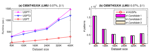
Figure 6. Scalability of the compared approaches.

As shown in Fig. 6, the USPT algorithm has obtained better results in terms of scalability than that of the USPT1 and USPT2 algorithms. With the increasing dataset size, the runtime and the number of candidates of USPT1, USPT2, and USPT increase as well. However, the runtime gap between USPT and USPT1 has become larger along with the increased dataset size. This is reasonable since when the size of dataset has become larger or more denser, more candidates in transactions are required to be determined for mining the HUSPs. This process leads to an increasing in the requirements of runtime consumption. Without the designed strategies to efficiently prune the redundant candidates in the search space, the baseline algorithm sometimes requires a long time to perform the mining process. As shown in Fig. 6(b), the size of the candidates remains stable along with the size of the dataset. The reason is that when the minimum utility value increases along with the dataset size, fewer candidates satisfy the condition for being HUSPs. If the data distribution in datasets was uniform, the number of candidates would increase or decrease steadily. However, the results in Fig. 6(b) shows that the datasets had no uniformity in data distribution. A computation to examine the candidates was still required, and the runtime increases along with the increasing size of the dataset.

7. Conclusion and Future Works

To solve utility-oriented sequential pattern mining, we presented a new USPT framework for efficiently discovering the set of HUSPs across multi-sequences by regarding individualized minimum utility thresholds, which are more informative and useful for decision makers, managers, and experts. To the best of our knowledge, this is the first study for solving the USPT problem. By utilizing the developed properties of upper-bounds, LS-tree and utility-array structures, the USPT framework was first proposed to extract the complete set of HUSPs. By utilizing the properties of various upper-bounds, three strategies were designed to prune the search space and improve the mining performance. To show the effectiveness and efficiency of the designed USPT algorithm, several experiments were conducted.

Since this is the first study on utility mining across multi-sequences with individualized thresholds, many extensions could be explored and studied in the future, such as designing more efficient algorithms, applying the proposed USPT algorithm in big data (Gan et al., 2017), or extending the USPT model to other interesting applications (e.g., discovering rare pattern (Koh and Ravana, 2016), parallel mining (Gan et al., 2019b), privacy preserving utility mining (Gan et al., 2018a), and recommender system (Yin et al., 2014)). Moreover, mining HUSPs with individualized thresholds over uncertain data (Lin et al., 2016a) would be a non-trivial and challenging task.

8. Acknowledgment

We sincerely thank the editors and anonymous reviewers whose valuable comments helped us to improve this paper significantly. This research was partially supported by the Shenzhen Technical Project under KQJSCX 20170726103424709 and JCYJ 20170307151733005, and NSF under grants III-1526499, III-1763325, III-1909323, SaTC-1930941, and CNS-1626432. Specifically, Wensheng Gan was supported by the China Scholarship Council Program, during his study at University of Illinois at Chicago, IL, USA.

References

- (1)
- Agrawal et al. (1993) Rakesh Agrawal, Tomasz Imielinski, and Arun Swami. 1993. Database mining: A performance perspective. IEEE Transactions on Knowledge and Data Engineering 5, 6 (1993), 914–925.
- Agrawal and Srikant (1994) Rakesh Agrawal and Ramakrishnan Srikant. 1994. Quest synthetic data generator. http://www.Almaden.ibm.com/cs/quest/syndata.html. (1994).
- Agrawal and Srikant (1995) Rakesh Agrawal and Ramakrishnan Srikant. 1995. Mining sequential patterns. In Proceedings of the International Conference on Data Engineering. IEEE, 3–14.
- Agrawal et al. (1994) Rakesh Agrawal, Ramakrishnan Srikant, et al. 1994. Fast algorithms for mining association rules. In Proceedings of the 20th International Conference on Very Large Data Bases, Vol. 1215. 487–499.
- Ahmed et al. (2010a) Chowdhury-Farhan Ahmed, Syed-Khairuzzaman Tanbeer, and Byeong-Soo Jeong. 2010a. Mining high utility web access sequences in dynamic web log data. In 11th ACIS International Conference on Software Engineering, Artificial Intelligence, Networking and Parallel/Distributed Computing. IEEE, 76–81.
- Ahmed et al. (2010b) Chowdhury-Farhan Ahmed, Syed-Khairuzzaman Tanbeer, and Byeong-Soo Jeong. 2010b. A novel approach for mining high-utility sequential patterns in sequence databases. ETRI Journal 32, 5 (2010), 676–686.
- Ahmed et al. (2009) Chowdhury-Farhan Ahmed, Syed-Khairuzzaman Tanbeer, Byeong-Soo Jeong, and Young-Koo Lee. 2009. Efficient tree structures for high utility pattern mining in incremental databases. IEEE Transactions on Knowledge and Data Engineering 21, 12 (2009), 1708–1721.
- Alkan and Karagoz (2015) Oznur Kirmemis Alkan and Pinar Karagoz. 2015. CRoM and HuspExt: Improving efficiency of high utility sequential pattern extraction. IEEE Transactions on Knowledge and Data Engineering 27, 10 (2015), 2645–2657.
- Ayres et al. (2002) Jay Ayres, Jason Flannick, Johannes Gehrke, and Tomi Yiu. 2002. Sequential pattern mining using a bitmap representation. In Proceedings of the 8th ACM SIGKDD International Conference on Knowledge Discovery and Data Mining. ACM, 429–435.
- Chan et al. (2003) Raymond Chan, Qiang Yang, and Yi Dong Shen. 2003. Mining high utility itemsets. In Proceedings of the 3rd IEEE International Conference on Data Mining. IEEE, 19–26.
- Chen et al. (1996) Ming-Syan Chen, Jiawei Han, and Philip S. Yu. 1996. Data mining: an overview from a database perspective. IEEE Transactions on Knowledge and Data Engineering 8, 6 (1996), 866–883.
- Fournier-Viger et al. (2017) Philippe Fournier-Viger, Jerry Chun-Wei Lin, Rage-Uday Kiran, and Yun-Sing Koh. 2017. A survey of sequential pattern mining. Data Science and Pattern Recognition 1, 1 (2017), 54–77.
- Fournier-Viger et al. (2014) Philippe Fournier-Viger, Cheng-Wei Wu, Souleymane Zida, and Vincent S Tseng. 2014. FHM: Faster high-utility itemset mining using estimated utility co-occurrence pruning. In International Symposium on Methodologies for Intelligent Systems. Springer, 83–92.
- Gan et al. (2018a) Wensheng Gan, Jerry Chun-Wei Lin, Han-Chieh Chao, Shyue-Liang Wang, and Philip S Yu. 2018a. Privacy preserving utility mining: a survey. In Proceedings of the IEEE International Conference on Big Data. IEEE, 2617–2626.
- Gan et al. (2017) Wensheng Gan, Jerry Chun-Wei Lin, Han-Chieh Chao, and Justin Zhan. 2017. Data mining in distributed environment: a survey. Wiley Interdisciplinary Reviews: Data Mining and Knowledge Discovery 7, 6 (2017), e1216.
- Gan et al. (2016) Wensheng Gan, Jerry Chun-Wei Lin, Philippe Fournier-Viger, and Han-Chieh Chao. 2016. More efficient algorithms for mining high-utility itemsets with multiple minimum utility thresholds. In International Conference on Database and Expert Systems Applications. Springer, 71–87.
- Gan et al. (2018b) Wensheng Gan, Jerry Chun-Wei Lin, Philippe Fournier-Viger, Han-Chieh Chao, Tzung-Pei Hong, and Hamido Fujita. 2018b. A survey of incremental high-utility itemset mining. Wiley Interdisciplinary Reviews: Data Mining and Knowledge Discovery 8, 2 (2018), e1242.
- Gan et al. (2019c) Wensheng Gan, Jerry Chun-Wei Lin, Philippe Fournier-Viger, Han-Chieh Chao, Vincent S Tseng, and Philip S Yu. 2019c. A survey of utility-oriented pattern mining. IEEE Transactions on Knowledge and Data Engineering, DOI: 10.1109/TKDE.2019.2942594 (2019), 1–22.
- Gan et al. (2019a) Wensheng Gan, Jerry Chun-Wei Lin, Philippe Fournier-Viger, Han-Chieh Chao, and Philip S Yu. 2019a. HUOPM: High-utility occupancy pattern mining. IEEE Transactions on Cybernetics, DOI: 10.1109/TCYB.2019.2896267 (2019), 1–14.
- Gan et al. (2019b) Wensheng Gan, Jerry Chun-Wei Lin, Philippe Fournier-Viger, Han-Chieh Chao, and Philip S Yu. 2019b. A survey of parallel sequential pattern mining. ACM Transactions on Knowledge Discovery from Data 13, 3 (2019), 25.
- Gan et al. (2019d) Wensheng Gan, Jerry Chun-Wei Lin, Zhang Jiexiong, Han-Chieh Chao, Hamido Fujita, and Philip S Yu. 2019d. ProUM: High utility sequential pattern mining. In Proceedings of the IEEE International Conference on Systems, Man, and Cybernetics. IEEE, 767–773.
- Han et al. (2004) Jiawei Han, Jian Pei, Yiwen Yin, and Runying Mao. 2004. Mining frequent patterns without candidate generation: A frequent-pattern tree approach. Data Mining and Knowledge Discovery 8, 1 (2004), 53–87.
- Hu et al. (2013) Ya-Han Hu, Fan Wu, and Yi-Jiun Liao. 2013. An efficient tree-based algorithm for mining sequential patterns with multiple minimum supports. Journal of Systems and Software 86, 5 (2013), 1224–1238.
- Koh and Ravana (2016) Yun-Sing Koh and Sri-Devi Ravana. 2016. Unsupervised rare pattern mining: a survey. ACM Transactions on Knowledge Discovery from Data 10, 4 (2016), 45.
- Krishnamoorthy (2018) Srikumar Krishnamoorthy. 2018. Efficient mining of high utility itemsets with multiple minimum utility thresholds. Engineering Applications of Artificial Intelligence 69 (2018), 112–126.
- Lan et al. (2011) Guo-Cheng Lan, Tzung-Pei Hong, and Vincent S Tseng. 2011. Discovery of high utility itemsets from on-shelf time periods of products. Expert Systems with Applications 38, 5 (2011), 5851–5857.
- Lan et al. (2014) Guo-Cheng Lan, Tzung-Pei Hong, Vincent S Tseng, and Shyue-Liang Wang. 2014. Applying the maximum utility measure in high utility sequential pattern mining. Expert Systems with Applications 41, 11 (2014), 5071–5081.
- Lee et al. (2009) Anthony JT Lee, Huei-Wen Wu, Tzu-Yu Lee, Ying-Ho Liu, and Kuo-Tay Chen. 2009. Mining closed patterns in multi-sequence time-series databases. Data & Knowledge Engineering 68, 10 (2009), 1071–1090.
- Lin et al. (2011) Chun-Wei Lin, Tzung-Pei Hong, and Wen-Hsiang Lu. 2011. An effective tree structure for mining high utility itemsets. Expert Systems with Applications 38, 6 (2011), 7419–7424.
- Lin et al. (2016a) Jerry Chun-Wei Lin, Wensheng Gan, Philippe Fournier-Viger, Tzung-Pei Hong, and Vincent S Tseng. 2016a. Efficient algorithms for mining high-utility itemsets in uncertain databases. Knowledge-Based Systems 96 (2016), 171–187.
- Lin et al. (2016b) Jerry Chun-Wei Lin, Wensheng Gan, Philippe Fournier-Viger, Tzung-Pei Hong, and Justin Zhan. 2016b. Efficient mining of high-utility itemsets using multiple minimum utility thresholds. Knowledge-Based Systems 113 (2016), 100–115.
- Lin et al. (2015a) Jerry Chun-Wei Lin, Wensheng Gan, and Tzung-Pei Hong. 2015a. A fast updated algorithm to maintain the discovered high-utility itemsets for transaction modification. Advanced Engineering Informatics 29, 3 (2015), 562–574.
- Lin et al. (2015b) Jerry Chun-Wei Lin, Wensheng Gan, Tzung-Pei Hong, and Vincent S Tseng. 2015b. Efficient algorithms for mining up-to-date high-utility patterns. Advanced Engineering Informatics 29, 3 (2015), 648–661.
- Lin et al. (2017) Jerry Chun-Wei Lin, Jiexiong Zhang, and Philippe Fournier-Viger. 2017. High-utility sequential pattern mining with multiple minimum utility thresholds. In Asia-Pacific Web and Web-Age Information Management Joint Conference on Web and Big Data. Springer, 215–229.
- Liu et al. (1999) Bing Liu, Wynne Hsu, and Yiming Ma. 1999. Mining association rules with multiple minimum supports. In Proceedings of the Fifth ACM SIGKDD International Conference on Knowledge Discovery and Data Mining. ACM, 337–341.
- Liu and Qu (2012) Mengchi Liu and Junfeng Qu. 2012. Mining high utility itemsets without candidate generation. In Proceedings of the 21st ACM International Conference on Information and Knowledge Management. ACM, 55–64.
- Liu et al. (2005) Ying Liu, Wei-Keng Liao, and Alok Choudhary. 2005. A two-phase algorithm for fast discovery of high utility itemsets. In Pacific-Asia Conference on Knowledge Discovery and Data Mining. Springer, 689–695.
- Liu et al. (2011) Yu-Cheng Liu, Chun-Pei Cheng, and Vincent S Tseng. 2011. Discovering relational-based association rules with multiple minimum supports on microarray datasets. Bioinformatics 27, 22 (2011), 3142–3148.
- Mai et al. (2017) Thang Mai, Bay Vo, and Loan TT Nguyen. 2017. A lattice-based approach for mining high utility association rules. Information Sciences 399 (2017), 81–97.
- Mannila et al. (1997) Heikki Mannila, Hannu Toivonen, and A Inkeri Verkamo. 1997. Discovery of frequent episodes in event sequences. Data Mining and Knowledge Discovery 1, 3 (1997), 259–289.
- Marshall (2005) Alfred Marshall. 2005. From Principles of Economics. In Readings in the Economics of the Division of Labor: the Classical Tradition. World Scientific, 195–215.
- Pei et al. (2001) Jian Pei, Jiawei Han, Behzad Mortazavi-Asl, Helen Pinto, Qiming Chen, Umeshwar Dayal, and Mei Chun Hsu. 2001. PrefixSpan: Mining sequential patterns efficiently by prefix-projected pattern growth. In The International Conference on Data Engineering. IEEE, 215–224.
- Pinto et al. (2001) Helen Pinto, Jiawei Han, Jian Pei, Ke Wang, Qiming Chen, and Umeshwar Dayal. 2001. Multi-dimensional sequential pattern mining. In Proceedings of the 10th International Conference on Information and Knowledge Management. ACM, 81–88.
- Ryang and Yun (2016) Heungmo Ryang and Unil Yun. 2016. High utility pattern mining over data streams with sliding window technique. Expert Systems with Applications 57 (2016), 214–231.
- Shie et al. (2011) Bai-En Shie, Hui-Fang Hsiao, Vincent S Tseng, and Philip S Yu. 2011. Mining high utility mobile sequential patterns in mobile commerce environments. In Proceedings of International Conference on Database Systems for Advanced Applications. Springer, 224–238.
- Srikant and Agrawal (1996) Ramakrishnan Srikant and Rakesh Agrawal. 1996. Mining sequential patterns: generalizations and performance improvements. In Proceedings of International Conference on Extending Database Technology. Springer, 1–17.
- Tseng et al. (2013) Vincent S Tseng, Bai-En Shie, Cheng-Wei Wu, and Philip S Yu. 2013. Efficient algorithms for mining high utility itemsets from transactional databases. IEEE Transactions on Knowledge and Data Engineering 25, 8 (2013), 1772–1786.
- Tseng et al. (2015) Vincent S Tseng, Cheng-Wei Wu, Philippe Fournier-Viger, and Philip S Yu. 2015. Efficient algorithms for mining the concise and lossless representation of high utility itemsets. IEEE Transactions on Knowledge and Data Engineering 27, 3 (2015), 726–739.
- Tseng et al. (2016) Vincent S Tseng, Cheng-Wei Wu, Philippe Fournier-Viger, and Philip S Yu. 2016. Efficient algorithms for mining top- high utility itemsets. IEEE Transactions on Knowledge and Data Engineering 28, 1 (2016), 54–67.
- Tseng et al. (2010) Vincent S Tseng, Cheng-Wei Wu, Bai-En Shie, and Philip S Yu. 2010. UP-Growth: an efficient algorithm for high utility itemset mining. In Proceedings of the 16th ACM SIGKDD International Conference on Knowledge Discovery and Data Mining. ACM, 253–262.
- Wang and Huang (2018) Jun-Zhe Wang and Jiun-Long Huang. 2018. On incremental high utility sequential pattern mining. ACM Transactions on Intelligent Systems and Technology 9, 5 (2018), 55.
- Wang et al. (2016) Jun-Zhe Wang, Jiun-Long Huang, and Yi-Cheng Chen. 2016. On efficiently mining high utility sequential patterns. Knowledge and Information Systems 49, 2 (2016), 597–627.
- Yao et al. (2004) Hong Yao, Howard J Hamilton, and Cory J Butz. 2004. A foundational approach to mining itemset utilities from databases. In Proceedings of the SIAM International Conference on Data Mining. SIAM, 482–486.
- Yin et al. (2014) Hongzhi Yin, Bin Cui, Yizhou Sun, Zhiting Hu, and Ling Chen. 2014. LCARS: A spatial item recommender system. ACM Transactions on Information Systems 32, 3 (2014), 11.
- Yin et al. (2012) Junfu Yin, Zhigang Zheng, and Longbing Cao. 2012. USpan: an efficient algorithm for mining high utility sequential patterns. In Proceedings of the 18th ACM SIGKDD International Conference on Knowledge Discovery and Data Mining. ACM, 660–668.
- Yin et al. (2013) Junfu Yin, Zhigang Zheng, Longbing Cao, Yin Song, and Wei Wei. 2013. Efficiently mining top- high utility sequential patterns. In Proceedings of the IEEE 13th International Conference on Data Mining. IEEE, 1259–1264.
- Yu and Chen (2005) Chung-Ching Yu and Yen-Liang Chen. 2005. Mining sequential patterns from multidimensional sequence data. IEEE Transactions on Knowledge and Data Engineering 17, 1 (2005), 136–140.
- Yun et al. (2017) Unil Yun, Gangin Lee, and Eunchul Yoon. 2017. Efficient high utility pattern mining for establishing manufacturing plans with sliding window control. IEEE Transactions on Industrial Electronics 64, 9 (2017), 7239–7249.
- Zaki (2001) Mohammed J Zaki. 2001. SPADE: an efficient algorithm for mining frequent sequences. Machine Learning 42, 1-2 (2001), 31–60.
- Zida et al. (2015) Souleymane Zida, Philippe Fournier-Viger, Jerry Chun-Wei Lin, Cheng-Wei Wu, and Vincent S Tseng. 2015. EFIM: a highly efficient algorithm for high-utility itemset mining. In Mexican International Conference on Artificial Intelligence. Springer, 530–546.