Improving Visual Recognition using Ambient Sound for Supervision

Abstract

Our brains combine vision and hearing to create a more elaborate interpretation of the world. When the visual input is insufficient, a rich panoply of sounds can be used to describe our surroundings. Since more than $1,000$ hours of videos are uploaded to the internet everyday, it is arduous, if not impossible, to manually annotate these videos. Therefore, incorporating audio along with visual data without annotations is crucial for leveraging this explosion of data for recognizing and understanding objects and scenes. [24] suggests that a rich representation of the physical world can be learned by using a convolutional neural network to predict sound textures associated with a given video frame. We attempt to reproduce the claims from their experiments, of which the code is not publicly available. In addition, we propose improvements in the pretext task that result in better performance in other downstream computer vision tasks.

Keywords: self-supervision, multi-modal learning, computer vision

1 Introduction

When there is movement, there is sound. One of the most important functions of the midbrain is the integration between visual and auditory signals through the corpora quadrigemina. In particular, the upper layers of the superior colliculi receive information from the retina and the central nuclei of inferior colliculi receive signals from multiple auditory receptors. Then, the lower layers of the superior colliculi and the central nuclei of inferior colliculi create an audiovisual loop, where the information is learned together dynamically. [31] suggests that by incorporating visual and auditory information, we learn a more accurate perception of the world. As a result, it is natural to question the sufficiency of unimodal computer vision algorithms in interpreting the complex world we experience.

On the other hand, since the invention of the convolutional neural network [35] and other deep learning techniques, we are able to create highly accurate supervised models that perform many computer vision tasks exceptionally well. However, training these models can be very expensive since labeling data requires exceedingly large amount of human effort and time. Alternatively, self-supervised learning has gained popularity over the past few years. It is cost-effective and it can be generalized to a multitude of downstream tasks.

In this paper, we present a self-supervised model that learns representations of the world using statistical summaries of sound textures extracted from audio associated with the frames in videos. We then evaluate the model performance by fine-tuning the model for object classification and compare the results to those from the current state-of-the-art models.

2 Related Work

Sound representation. A sound texture is a composition of acoustic features. Many studies have been done to create different representations of sound textures such as Markov model-based clustering [18] and support vector machine [20]. In our paper, however, we focused on representing sound textures using statistical summaries. Several works have approached sound representations and shown interesting results [8, 10]. We are particularly interested in the statistical model described in [21].

Multi-modal learning. In a multi-model learning algorithm, more than one modality is incorporated in the learning process. For instance, [30] uses a deep Boltzmann machine to learn molti-modal data and [14] uses images and natural language data to create bidirectional retrieval mappings between them. A detailed list of multi-modal works can be found in [2]. We attempt to combine sound and visual data in hope to provide insights on computer vision tasks because it mimics how we perceive and learn the world.

Self-supervised Learning. Self-supervised learning has been able to discover natural features in the data. Many different supervisions have been proposed: [32] uses video tracking as supervision, [13] uses rate of co-occurrence in space and time as supervision. We use sound for supervision because sound provides rich information that are lacked from still images.

3 Approach

3.1 Dataset

We want to create a model which given an image, predicts the corresponding sound. For this, we use a subset of the AudioSet dataset [11] which contains $10$-second video clips. We prefer to use AudioSet over other video datasets such as Kinetics [15] because videos in AudioSet have more local sound as opposed to background music that is counter-intuitive to our approach. We assume that the ambient sound caused by objects in the frame will help the model gain a better visual understanding as opposed to noise, such as from music videos.

Although the AudioSet contains videos, we want to predict sound from only the given frame. This ensures that the learned image features can then be used for image recognition downstream tasks that will be discussed later in this paper. We then choose to use $3.75$-second clips of audios for their corresponding image frames as it has been shown that sound is temporally invariant in this window [21]. Finally, we obtain around $55,000$ frames with their corresponding audio clips.

3.2 Representing Sound

Statistical Summaries of Sound. We follow closely the method suggested in [24], a modified version of [21], to compute a set of $502$-dimensional vectors of statistical summaries of the audio clips. We describe the method briefly as follows. To obtain a set of $32$ subband envelopes, a sound waveform $\bm{s}$ is convoluted with a bank $\left\{\bm{f_{i}}\right\}_{i=1}^{32}$ of bandpass filters

$$c_{i}(t)=\left|(\bm{s}\ast\bm{f}_{i})+i\mathcal{H}(\bm{s}\ast\bm{f}_{i})\right|$$

where $\mathcal{H}$ denotes the Hilbert transform, $i=\sqrt{-1}$, and $\ast$ is the convolution operator. The subband envelopes are then downsampled to $400$ Hz for computational efficiency and raised to $0.3$ power to simulate basilar membrane compression [21]. Next, we compute several statistics for the subband envelopes. First, we estimate the marginal statistics, i.e. the means $\left\{\mu_{i}\right\}_{i=1}^{32}$ and the standard deviations $\left\{\sigma_{i}\right\}_{i=1}^{32}$ for each subband envelope $c_{i}(t)$, and normalize the standard deviations $\tilde{\sigma}_{i}=\sqrt{\sigma_{i}^{2}/\mu_{i}^{2}}$. Then, we compute the cross-band envelope correlations

$$\rho_{jk}=\sum_{t}\frac{(c_{j}(t)-\mu_{j})(c_{k}(t)-\mu_{k})}{\sigma_{j}\sigma_{k}}$$

for all $j,k\in[1,\ldots,32]$ such that $\left|j-k\right|\in\left\{1,2,3,5\right\}$. Lastly, we calculate the loudness $l=\mathrm{median}({\left\|\bm{c}(t)\right\|})$ of the subband envelopes. On the other hand, we estimate modulation filters by convoluting the subband envelopes with a bank $\left\{\bm{m_{j}}\right\}_{j=1}^{10}$ of bandpass filters

$$b_{ij}=\frac{{\left\|c_{i}\ast m_{j}\right\|}^{2}}{N},$$

where $N$ is the length of the modulation filters. The $b_{ij}$’s are then normalized by the same variance of the subband envelope $\tilde{b}_{ij}=\sqrt{b_{ij}/\mu_{i}^{2}}$. Lastly, we flatten the vectors and matrices and organize these statistics into the desired summary vector

$$(\mu_{1},\ldots,\mu_{32},\tilde{\sigma_{1}},\ldots,\tilde{\sigma}_{32},\rho_{1},,\ldots,\rho_{32},\tilde{b}_{1},\ldots,\tilde{b}_{320},l)\in\mathbb{R}^{502}.$$

Mel-Frequency Cepstral Coefficents (MFCCs). In addition to the statistical summaries of sound used in [24], we create a second set of acoustic representations using MFCCs [5]. MFCCs has been a standard method to represent sound parametrically since its invention. MFCCs first low-pass filter a sound waveform $\bm{s}$ at $5$ kHz and then sample at $10$ kHz. Next, $20$ triangular bandpass filters are used to compute MFCCs for cascaded frames $12.8$ ms apart with a $256$ Hamming window using discrete Fourier transform

$$\mathrm{MFCC}_{i}=\sum_{k=1}^{20}X_{k}\cos\left[i\left(k-\frac{1}{2}\right)\frac{\pi}{20}\right],$$

where $i=1,\ldots,155$ and $X_{k}$ is the log-energy output of the $k$th filter. For simplicity, we use MFCC from Librosa [4] and obtain a set of $20\times 155$ matrices and flatten them into vectors of size $3,100$.

3.3 Predicting sound from images

Now that we have a set of supervisory signal vectors, we treat our problem as a regression task and predict sound vectors from images themselves using a deep convolutional neural network. However, the difficulty in training such a model has been highlighted before by Owens et al in [24]. Hence, using a classification approach would be a much more lucrative option as it makes analysis of the model easier. So, we use the clustering approach as described in [24], where we perform $k$-means clustering on the entire dataset and categorize each frame and its corresponding audio into a cluster. These different clusters can then act as output classes which can be used as the supervisory signals while training the model.

We perform the same clustering on both representations of sound (Statistical summaries and MFCCs).

The idea behind clustering frames based on their sound is that frames belonging to the same cluster would contain similar sounding objects in them. Using these clusters as our supervisory signals would help our model learn to differentiate between these clusters, and in turn, the different objects in them. These similarities can be seen in Figure 1.

Figure 1: (Left) Frames grouped by sound clusters. We see that frames from videos fall into categories such as “outdoor scenes”, “indoor scenes”, “people laughing”, and “music”. (Right) Our sound prediction model.

Self-supervised training

We use an AlexNet model [17], which takes in a single RGB frame as input and predicts the corresponding cluster number (which we will call as the “class”). We use PyTorch [25] to train this model and cross-entropy loss to calculate the error between the predicted and the true class. We use the AdamW [28] optimizer along with the OneCycle learning rate scheduling policy [29] for $200$ epochs.

An interesting question arises while training this pretext model is that to what extent should we train the model? If the model gets very good at classifying these sound clusters, it can prove degrading towards the downstream tasks. As a result, we choose to train the model for a fixed number of iterations ($200$), which usually gives us a validation set classification accuracy of nearly $45\%-55\%$ depending on the number of clusters.

Filter $\bm{7}$

Filter $\bm{23}$

Filter $\bm{117}$

Filter $\bm{129}$

Filter $\bm{205}$

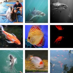
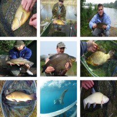
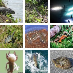
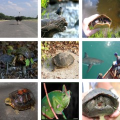
Figure 2: Top activated images from a subset of the dataset for a specific target filters in the 3rd convolutional layer. We see that the images contain different objects in the same scene, like, fishes in water, people holding caught fish, or insects on the ground.

4 Evaluation of trained model

Qualitative evaluation:

A good way to assess what the model has learned is to learn which input image maximizes the activation of a particular neuron in the model. This method has been described in detail in [37] and [9]. Figure 2 shows the top $9$ activated images from a subset of our dataset. An interesting observation that emerges is that backgrounds of images in a given set are the same even if the objects in the foregrounds are different.

We suspect that this indicates the fact that backgrounds contribute more to the ambient sound. This still means that the model has learned a rich representation of the world. It can be demonstrated further by using this model to fine-tune for other downstream tasks.

Quantitative - Finetuning on Pascal VOC:

We evaluate our model quantitatively by fine-tuning it on image classification on Pascal VOC. The training set of Pascal VOC contains $2500$ images which makes it an ideal candidate for evaluation as it is very close to real world situations where obtaining a lot of labeled data is difficult. We follow the standard testing conditions for classification on the test set of Pascal VOC 2007 dataset and perform hyperparameter tuning on the validation set.

We perform two different fine-tuning experiments, one where we only train the “head” of the model while we freeze the rest of it. And the other where we fine-tune the whole model.

Table 1 summarizes and compares the mean average precision percentages between our approach and other self-supervised approaches. We use our $15$-cluster variant of the model for the comparisons.

	Head	All
Imagenet(pretrained) [17]	78.9	79.9
Random [16]	29	33.2
Pathak et al. [27]	34.6	56.5
Donahue et al. [7]	52.3	60.1
Owens et al. [24]	52.3	61.3
Pathak et al. [26]	-	61
Wang et al. [33]	55.6	63.1
Doersch et al. [6]	55.1	65.3
Bojanowski et al. [3]	56.7	65.3
Zhang et al. [38]	61.5	65.9
Zhang et al. [39]	63	67.1
Noroozi and Favaro [22]	-	67.6
Noroozi et al. [23]	-	67.7
Our model	52.8	55.1

Table 1: Comparison of the statistical summaries Alexnet model with $15$ clusters to the state-of-the-art unsupervised approaches on Pascal VOC classification. Here, “Head” refers to training only the fully connected part of the model, and “All” refers to fine-tuning the entire model.

5 Further experiments

ResNet vs AlexNet: We hypothesize that using a ResNet model, which is proven to have a higher learning capacity, would be more beneficial for this task. Hence, we follow the same procedure and evaluate the performance on the ResNet-18 variant and we compare the results with the AlexNet model. We find that the AlexNet outperforms ResNet-18, which could be attributed to the fact that the ResNet model requires more training than the AlexNet model to learn a better visual representation. However, when trained for the same amount of epochs, AlexNet seems to learn a better representation.

Varying cluster sizes: We investigate how varying cluster sizes affects the performance of the model on the downstream task. As shown in Figure 3 We find that there is little improvement past $30$ clusters, whereas having very few clusters is also not ideal to produce good performance.

This trend is carried over when we use a ResNet model, which tells us that cluster sizes are independent of the model we use to train our pretext task.

	aer	bk	brd	bt	btl	bus	car	cat	chr	cow	din	dog	hrs	mbk	prs	pot	shp	sfa	trn	tv
Imagenet(pretrained)[17]	79	71	73	75	25	60	80	75	51	45	60	70	80	72	91	42	62	56	82	62
Owens et al. [24]	68	47	38	54	15	45	66	45	42	23	37	28	71	58	85	25	26	32	67	42
Colorization [38]	70	50	45	58	15	45	71	50	39	20	38	41	72	57	81	17	42	41	66	38
Tracking [33]	67	35	41	54	11	35	62	35	39	21	30	26	70	53	78	22	32	37	61	34
Object motion [26]	65	39	39	50	13	33	61	36	39	24	35	28	69	49	82	14	19	34	56	31
Patch position [6]	70	44	43	60	12	44	66	52	44	24	45	31	73	48	78	14	28	39	62	43
Egomotion [1]	60	24	21	35	10	19	57	24	27	11	22	18	61	40	69	13	12	24	48	28
Texton-CNN [19]	65	35	28	46	11	31	63	30	41	17	28	23	64	51	74	9	19	33	54	30
$k$-means [16]	61	31	27	69	9	27	58	34	36	12	25	21	64	38	70	18	14	25	51	25
Ours - Sound Texture	76	58	45	57	20	60	76	48	44	35	46	42	75	69	90	33	34	43	76	43
Ours - MFCC	74	60	48	57	20	54	76	49	45	37	51	43	74	69	87	31	40	42	75	45

Table 2: Per class AP score on the Pascal VOC classification task. The average of these $20$ scores represents the mAP of the model.

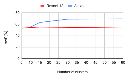
Figure 3: (Left) Difference in the mean average precision obtained from two different model architectures keeping cluster size fixed at $15$. (Right) Effects of varying the cluster sizes on the two kinds of models.

Statistical summaries vs MFCC: We choose MFCCs as an alternative sound representation. To see how the learned representation varies, we evaluate the mAP on the downstream image classification task on Pascal VOC in a similar manner using the model trained with the MFCC features. Figure 4 shows the comparison between statistical summaries and MFCC features on the downstream task. We can see that there is a slight improvement using MFCCs. This can be attributed to the different representation of the sound which leads to a different clustering, which then in turn lead to a different visual representation learned by the model.

Figure 4: Comparing the mAP on the downstream task by models learned using Statistical summaries vs MFCCs as the audio representation.

6 Discussion

We see that the representation of sound matters significantly in this study. Hence, looking for an optimal sound representation will be crucial to advances in this approach. A case can be made for learning these audio representations using deep neural networks as shown in [12]. However, since they would be trained using human annotated labels, they would not be in the spirit of a truly self-supervised approach.

The effects of using deeper networks like Wide-Resnets [36] and ResNeXts [34], which currently are the state-of-the-art models for image recognition, can also be studied. However, their performance need not be analogous as seen here by the comparison between ResNet-18 and AlexNet.

Other self-supervised techniques are evaluated on different downstream tasks such as bounding box detection and instance segmentation as well. This means that visual representations obtained in this manner are rich enough to translate to several different tasks and the limits of which can be further studied.

7 Conclusion

In this paper, we showed a scalable approach for training self-supervised models on image recognition tasks using audios as supervisory signals. We successfully reproduced the claims in [24]. Additionally, we observed that using different representations of audios can affect the performance on the downstream task and mel-frequency cepstral coefficents tend to perform better than statistical sound summaries. Our approach works best when the pretext task is trained on a dataset like AudioSet, where the sources of sound are local to the image. This approach is highly scalable due to the abundance of available videos and therefore making it a good candidate for learning deep representations in a self-supervised manner where obtaining human annotations is proven to be difficult.

References

- [1] Pulkit Agrawal, Joao Carreira, and Jitendra Malik. Learning to see by moving. In Proceedings of the IEEE International Conference on Computer Vision, pages 37–45, 2015.
- [2] Tadas Baltrušaitis, Chaitanya Ahuja, and Louis-Philippe Morency. Multimodal machine learning: A survey and taxonomy. IEEE Transactions on Pattern Analysis and Machine Intelligence, 41(2):423–443, 2018.
- [3] Piotr Bojanowski, Armand Joulin, David Lopez-Paz, and Arthur Szlam. Optimizing the latent space of generative networks. arXiv preprint arXiv:1707.05776, 2017.
- [4] Matt McVicar Alexandros Metsai Stefan Balke Carl Thomé Adam Weiss Brian McFee, Vincent Lostanlen. librosa/librosa: 0.7.1 (version 0.7.1)., 2019.
- [5] S. Davis and P. Mermelstein. Comparison of parametric representations for monosyllabic word recognition in continuously spoken sentences. IEEE Transactions on Acoustics, Speech, and Signal Processing, 28(4):357–366, August 1980.
- [6] Carl Doersch, Abhinav Gupta, and Alexei A Efros. Unsupervised visual representation learning by context prediction. In Proceedings of the IEEE International Conference on Computer Vision, pages 1422–1430, 2015.
- [7] Jeff Donahue, Philipp Krähenbühl, and Trevor Darrell. Adversarial feature learning. arXiv preprint arXiv:1605.09782, 2016.
- [8] D. P. W. Ellis, X. Zeng, and J. H. McDermott. Classifying soundtracks with audio texture features. In 2011 IEEE International Conference on Acoustics, Speech and Signal Processing (ICASSP), pages 5880–5883, May 2011.
- [9] Dumitru Erhan, Yoshua Bengio, Aaron Courville, and Pascal Vincent. Visualizing higher-layer features of a deep network. University of Montreal, 1341(3):1, 2009.
- [10] A. J. Eronen, V. T. Peltonen, J. T. Tuomi, A. P. Klapuri, S. Fagerlund, T. Sorsa, G. Lorho, and J. Huopaniemi. Audio-based context recognition. IEEE Transactions on Audio, Speech, and Language Processing, 14(1):321–329, Jan 2006.
- [11] Jort F Gemmeke, Daniel PW Ellis, Dylan Freedman, Aren Jansen, Wade Lawrence, R Channing Moore, Manoj Plakal, and Marvin Ritter. Audio set: An ontology and human-labeled dataset for audio events. In 2017 IEEE International Conference on Acoustics, Speech and Signal Processing (ICASSP), pages 776–780. IEEE, 2017.
- [12] Shawn Hershey, Sourish Chaudhuri, Daniel P. W. Ellis, Jort F. Gemmeke, Aren Jansen, Channing Moore, Manoj Plakal, Devin Platt, Rif A. Saurous, Bryan Seybold, Malcolm Slaney, Ron Weiss, and Kevin Wilson. Cnn architectures for large-scale audio classification. In International Conference on Acoustics, Speech and Signal Processing (ICASSP). 2017.
- [13] Phillip Isola, Daniel Zoran, Dilip Krishnan, and Edward H Adelson. Learning visual groups from co-occurrences in space and time. arXiv preprint arXiv:1511.06811, 2015.
- [14] Andrej Karpathy, Armand Joulin, and Li F Fei-Fei. Deep fragment embeddings for bidirectional image sentence mapping. In Advances in neural information processing systems, pages 1889–1897, 2014.
- [15] Will Kay, Joao Carreira, Karen Simonyan, Brian Zhang, Chloe Hillier, Sudheendra Vijayanarasimhan, Fabio Viola, Tim Green, Trevor Back, Paul Natsev, et al. The kinetics human action video dataset. arXiv preprint arXiv:1705.06950, 2017.
- [16] Philipp Krähenbühl, Carl Doersch, Jeff Donahue, and Trevor Darrell. Data-dependent initializations of convolutional neural networks. arXiv preprint arXiv:1511.06856, 2015.
- [17] Alex Krizhevsky, Ilya Sutskever, and Geoffrey E Hinton. Imagenet classification with deep convolutional neural networks. In F. Pereira, C. J. C. Burges, L. Bottou, and K. Q. Weinberger, editors, Advances in Neural Information Processing Systems 25, pages 1097–1105. Curran Associates, Inc., 2012.
- [18] K. Lee, D. P. W. Ellis, and A. C. Loui. Detecting local semantic concepts in environmental sounds using markov model based clustering. In 2010 IEEE International Conference on Acoustics, Speech and Signal Processing, pages 2278–2281, March 2010.
- [19] Thomas Leung and Jitendra Malik. Representing and recognizing the visual appearance of materials using three-dimensional textons. International journal of computer vision, 43(1):29–44, 2001.
- [20] Lie Lu, HongJiang Zhang, and Stan Z. Li. Content-based audio classification and segmentation by using support vector machines. Multimedia Systems, 8:482–492, 2003.
- [21] Simoncelli E.P. McDermott, J.H. Sound texture perception via statistics of the auditory periphery: evidence from sound synthesis. volume 71(5), 926–940s, 2011.
- [22] Mehdi Noroozi and Paolo Favaro. Unsupervised learning of visual representations by solving jigsaw puzzles. In European Conference on Computer Vision, pages 69–84. Springer, 2016.
- [23] Mehdi Noroozi, Hamed Pirsiavash, and Paolo Favaro. Representation learning by learning to count. In Proceedings of the IEEE International Conference on Computer Vision, pages 5898–5906, 2017.
- [24] Andrew Owens, Jiajun Wu, Josh H McDermott, William T Freeman, and Antonio Torralba. Learning sight from sound: Ambient sound provides supervision for visual learning. In International Journal of Computer Vision (IJCV), 2018.
- [25] Adam Paszke, Sam Gross, Francisco Massa, Adam Lerer, James Bradbury, Gregory Chanan, Trevor Killeen, Zeming Lin, Natalia Gimelshein, Luca Antiga, et al. Pytorch: An imperative style, high-performance deep learning library. In Advances in Neural Information Processing Systems, pages 8024–8035, 2019.
- [26] Deepak Pathak, Ross Girshick, Piotr Dollár, Trevor Darrell, and Bharath Hariharan. Learning features by watching objects move. In Proceedings of the IEEE Conference on Computer Vision and Pattern Recognition, pages 2701–2710, 2017.
- [27] Deepak Pathak, Philipp Krahenbuhl, Jeff Donahue, Trevor Darrell, and Alexei A Efros. Context encoders: Feature learning by inpainting. In Proceedings of the IEEE conference on computer vision and pattern recognition, pages 2536–2544, 2016.
- [28] Sashank J Reddi, Satyen Kale, and Sanjiv Kumar. On the convergence of adam and beyond. arXiv preprint arXiv:1904.09237, 2019.
- [29] Leslie N Smith and Nicholay Topin. Super-convergence: Very fast training of residual networks using large learning rates. 2018.
- [30] Nitish Srivastava and Ruslan R Salakhutdinov. Multimodal learning with deep boltzmann machines. In Advances in neural information processing systems, pages 2222–2230, 2012.
- [31] Pieper F. Hollensteiner KJ. Engler G. Engel AK. Stitt I., Galindo-Leon E. Auditory and visual interactions between the superior and inferior colliculi in the ferret. volume 41. Issue 10. Page 1311 - 1320., 2015.
- [32] Xiaolong Wang and Abhinav Gupta. Unsupervised learning of visual representations using videos. In Proceedings of the IEEE International Conference on Computer Vision, pages 2794–2802, 2015.
- [33] Xiaolong Wang and Abhinav Gupta. Unsupervised learning of visual representations using videos. In Proceedings of the IEEE International Conference on Computer Vision, pages 2794–2802, 2015.
- [34] Saining Xie, Ross Girshick, Piotr Dollár, Zhuowen Tu, and Kaiming He. Aggregated residual transformations for deep neural networks. In Proceedings of the IEEE conference on computer vision and pattern recognition, pages 1492–1500, 2017.
- [35] Yoshua Bengio Patrick Haffner Yann LeCun, Léon Bottou. Gradient-based learning applied to document recognition. volume 86. Issue 11. Page 2278-2324, 1998.
- [36] Sergey Zagoruyko and Nikos Komodakis. Wide residual networks. arXiv preprint arXiv:1605.07146, 2016.
- [37] Matthew D Zeiler and Rob Fergus. Visualizing and understanding convolutional networks. In European conference on computer vision, pages 818–833. Springer, 2014.
- [38] Richard Zhang, Phillip Isola, and Alexei A Efros. Colorful image colorization. In ECCV, 2016.
- [39] Richard Zhang, Phillip Isola, and Alexei A Efros. Split-brain autoencoders: Unsupervised learning by cross-channel prediction. In Proceedings of the IEEE Conference on Computer Vision and Pattern Recognition, pages 1058–1067, 2017.