Learning performance in inverse Ising problems
with sparse teacher couplings

Alia Abbara, Yoshiyuki Kabashima, Tomoyuki Obuchi , and Yingying Xu Laboratoire de Physique de l’Ecole Normale Supérieure, 24 rue Lhomond, 75005 Paris, France Department of Mathematical and Computing Science, Tokyo Institute of Technology, 2-12-1, Ookayama, Meguro-ku, Tokyo, JapanDepartment of Systems Science, Graduate School of Informatics, Kyoto University, Yoshida Hon-machi, Sakyo-ku, Kyoto-shi, Kyoto 606-8501, JapanCorresponding author. E-mail: obuchi@@@i.kyoto-u.ac.jp
Abstract

We investigate the learning performance of the pseudolikelihood maximization method for inverse Ising problems. In the teacher-student scenario under the assumption that the teacher’s couplings are sparse and the student does not know the graphical structure, the learning curve and order parameters are assessed in the typical case using the replica and cavity methods from statistical mechanics. Our formulation is also applicable to a certain class of cost functions having locality; the standard likelihood does not belong to that class. The derived analytical formulas indicate that the perfect inference of the presence/absence of the teacher’s couplings is possible in the thermodynamic limit taking the number of spins N𝑁N as infinity while keeping the dataset size M𝑀M proportional to N𝑁N, as long as α=M/N>2𝛼𝑀𝑁2\alpha=M/N>2. Meanwhile, the formulas also show that the estimated coupling values corresponding to the truly existing ones in the teacher tend to be overestimated in the absolute value, manifesting the presence of estimation bias. These results are considered to be exact in the thermodynamic limit on locally tree-like networks, such as the regular random or Erdős–Rényi graphs. Numerical simulation results fully support the theoretical predictions. Additional biases in the estimators on loopy graphs are also discussed.

1 Introduction

Inference based on the classical Ising model is called the inverse Ising problem or Boltzmann machine learning, which is attracting more and more attention with the increasing interest in machine learning technologies. One recent application spurring this trend is for retinal neurons [1, 2], and subsequent applications to a wide range of systems have been conducted [3, 4, 5, 6, 7, 8, 9, 10], showing the potential usefulness of the inverse Ising framework.

However, it is difficult to compute standard estimators such as the maximum likelihood estimator in this framework when the system size is large. Thus, certain approximations and/or algorithms must be tailored to ease this difficulty and meet the demands of advanced applications, which have been attempted in previous studies [11, 12, 13, 14, 15, 16, 17, 18, 19, 20, 21, 22, 23]. One of the most effective examples is the pseudolikelihood method [11, 20]. This method approximates the likelihood function by the product of conditional likelihood functions, each of which is for a single random variable conditioned by its neighboring variables. This is useful for a wide range of problems defined on graphical models, and enables us to treat large systems because local couplings directly connected to a focused single random variable are isolated from the other couplings, and thus can be estimated independently. This local nature is sometimes referred to as local learning [24].

Another benefit of local learning is its theoretical tractability in high-dimensional settings. Recent theoretical analyses based on the replica method revealed the tight limit of inference accuracy in the thermodynamic limit where the dataset size is comparable to model dimensionality [24, 25, 26]. This provides a firm theoretical basis for the inverse Ising framework.

Previous studies of [24, 25, 26] focused on fully-connected Ising models. In high-dimensional settings, however, sparsely-connected models are more interesting because the inference accuracy is expected to be much better than the dense case, and the inferred estimator is expected to have clearer interpretations owing to the sparsity. The present paper deals with this case. We investigate the so-called teacher-student scenario using the replica method by drawing on previous studies [24, 25, 26], but refine the theoretical treatment in [24] for dealing with the teacher with sparse connections. The cavity method is used but the cavity field is assumed to consist of separately treatable signal and noise; the functional form of the associated probability distribution is hypothesized. The network structure of couplings is assumed to be locally tree-like, and our theoretical result is expected to be exact on those networks in the thermodynamic limit. To check the accuracy, numerical experiments are also conducted.

The remainder of this paper is organized as follows. In sec. 2, we review the inverse Ising framework and the statistical mechanical formulation to analyze inference accuracy. We also briefly review the analysis of the fully-connected case given in [24] to demonstrate how the formulation is applied. In sec. 3, we extend the method in the statistical mechanical formulation to the sparsely-connected case. Some theoretical treatments developed in [24] are refined and our ansatz to deal with the teacher model with sparse connections is stated. In sec. 4, our numerical analysis results are provided and compared with our theoretical results to check their accuracy. The final section presents a summary and discussion.

2 Formulation

In this section, we briefly review the inverse Ising framework and two associated inference methods: the maximum likelihood (ML) and pseudolikelihood (PL) methods. The class of local learning is also introduced and explained. In addition, the general framework of the statistical-mechanical analysis proposed in [24] is presented. We emphasize its technically important points and review the case of the fully-connected Ising model [24] to demonstrate its application.

2.1 Inference framework

Let us consider an Ising model consisting of N𝑁N spin variables 𝒔=(si=±1)i=1N𝒔superscriptsubscriptsubscript𝑠𝑖plus-or-minus1𝑖1𝑁\bm{s}=\left(s_{i}=\pm 1\right)_{i=1}^{N} and obeying the following distribution:

PIsing(𝒔|J,𝑯)=1ZIsingei<jNJijsisj+i=1NHisi,subscript𝑃Isingconditional𝒔𝐽𝑯1subscript𝑍Isingsuperscript𝑒superscriptsubscript𝑖𝑗𝑁subscript𝐽𝑖𝑗subscript𝑠𝑖subscript𝑠𝑗superscriptsubscript𝑖1𝑁subscript𝐻𝑖subscript𝑠𝑖\displaystyle P_{\rm Ising}\left(\bm{s}\big{|}J,\bm{H}\right)=\frac{1}{Z_{\rm Ising}}e^{\sum_{i<j}^{N}J_{ij}s_{i}s_{j}+\sum_{i=1}^{N}H_{i}s_{i}}, (1)

where JN×N𝐽superscript𝑁𝑁J\in\mathbb{R}^{N\times N} and 𝑯N𝑯superscript𝑁\bm{H}\in\mathbb{R}^{N} are termed couplings and external fields, respectively. The setting of the inverse Ising problem is aimed at inferring the couplings and external fields from a given dataset of spin snapshots (samples) DM{𝒔(μ)}μ=1Msuperscript𝐷𝑀superscriptsubscriptsuperscript𝒔𝜇𝜇1𝑀D^{M}\equiv\left\{\bm{s}^{(\mu)}\right\}_{\mu=1}^{M}, where M𝑀M denotes the dataset size. The representative statistical solution or estimator is the ML estimator defined by

{J^ML(DM),𝑯^ML(DM)}=argminJ,𝑯{μ=1MlogPIsing(𝒔(μ)|J,𝑯)}.superscript^𝐽MLsuperscript𝐷𝑀superscript^𝑯MLsuperscript𝐷𝑀subscriptargmin𝐽𝑯superscriptsubscript𝜇1𝑀subscript𝑃Isingconditionalsuperscript𝒔𝜇𝐽𝑯\displaystyle\left\{\hat{J}^{\rm ML}(D^{M}),\hat{\bm{H}}^{\rm ML}(D^{M})\right\}=\operatorname*{arg\,min}_{J,\bm{H}}\left\{-\sum_{\mu=1}^{M}\log P_{\rm Ising}\left(\bm{s}^{(\mu)}\big{|}J,\bm{H}\right)\right\}. (2)

Hereafter, the symbol ^^\hat{\cdot} is used to represent an estimator. This canonical estimator has some desirable properties such as consistency, unbiasedness, and efficiency when the dataset size M𝑀M is large enough while N𝑁N is kept finite (the asymptotic limit) [27, 28]. Consistency means that the estimator converges in probability to the true parameter in the large M𝑀M limit; unbiasedness means that the mean of the estimator (which is a random variable when the dataset is randomly generated) becomes identical to the true parameter; unbiased estimators yielding the lowest mean-squared error are termed efficient. Note that the ML estimator enjoys the unbiasedness and the efficiency only in the asymptotic sense, and for finite size datasets it can have bias and be not efficient.

In this sense, the ML estimator is good, but is not always appropriate for the inverse Ising framework for some computational reasons. The PL method [11] overcomes this problem by replacing the likelihood with the conditional distribution P(si|𝒔\i,𝑱i,Hi)𝑃conditionalsubscript𝑠𝑖subscript𝒔\absent𝑖subscript𝑱𝑖subscript𝐻𝑖P\left(s_{i}\big{|}\bm{s}_{\backslash i},\bm{J}_{i},H_{i}\right) for each sisubscript𝑠𝑖s_{i}, where 𝑱i=(Jij)jsubscript𝑱𝑖subscriptsubscript𝐽𝑖𝑗𝑗\bm{J}_{i}=(J_{ij})_{j} is the coupling vector connected to the i𝑖ith spin, and 𝒔\isubscript𝒔\absent𝑖\bm{s}_{\backslash i} denotes the spin vector without the i𝑖ith component. The explicit form is

P(si|𝒔\i,𝑱i,Hi)=1Ziesi(j(i)Jijsj+Hi),𝑃conditionalsubscript𝑠𝑖subscript𝒔\absent𝑖subscript𝑱𝑖subscript𝐻𝑖1subscript𝑍𝑖superscript𝑒subscript𝑠𝑖subscriptannotated𝑗absent𝑖subscript𝐽𝑖𝑗subscript𝑠𝑗subscript𝐻𝑖\displaystyle P\left(s_{i}\big{|}\bm{s}_{\backslash i},\bm{J}_{i},H_{i}\right)=\frac{1}{Z_{i}}e^{s_{i}\left(\sum_{j(\neq i)}J_{ij}s_{j}+H_{i}\right)}, (3)
Zi=2cosh(j(i)Jijsj+Hi).subscript𝑍𝑖2subscriptannotated𝑗absent𝑖subscript𝐽𝑖𝑗subscript𝑠𝑗subscript𝐻𝑖\displaystyle Z_{i}=2\cosh\left(\sum_{j(\neq i)}J_{ij}s_{j}+H_{i}\right). (4)

The PL estimator is obtained separately for each i𝑖i by

{𝑱^iPL(DM),H^iPL(DM)}=argmin𝑱i,Hi{μ=1MlogP(si(μ)|𝒔\i(μ),𝑱i,Hi)}subscriptsuperscript^𝑱PL𝑖superscript𝐷𝑀superscriptsubscript^𝐻𝑖PLsuperscript𝐷𝑀subscriptargminsubscript𝑱𝑖subscript𝐻𝑖superscriptsubscript𝜇1𝑀𝑃conditionalsubscriptsuperscript𝑠𝜇𝑖subscriptsuperscript𝒔𝜇\absent𝑖subscript𝑱𝑖subscript𝐻𝑖\displaystyle\left\{\hat{\bm{J}}^{\rm PL}_{i}(D^{M}),\hat{H}_{i}^{\rm PL}(D^{M})\right\}=\operatorname*{arg\,min}_{\bm{J}_{i},H_{i}}\left\{-\sum_{\mu=1}^{M}\log P\left(s^{(\mu)}_{i}\big{|}\bm{s}^{(\mu)}_{\backslash i},\bm{J}_{i},H_{i}\right)\right\}
=argmin𝑱i,Hi{μ=1MPL(si(μ)hi(𝒔\i(μ),𝑱i,Hi))},absentsubscriptargminsubscript𝑱𝑖subscript𝐻𝑖superscriptsubscript𝜇1𝑀superscriptPLsubscriptsuperscript𝑠𝜇𝑖subscript𝑖subscriptsuperscript𝒔𝜇\absent𝑖subscript𝑱𝑖subscript𝐻𝑖\displaystyle=\operatorname*{arg\,min}_{\bm{J}_{i},H_{i}}\left\{\sum_{\mu=1}^{M}\ell^{\rm PL}\left(s^{(\mu)}_{i}h_{i}(\bm{s}^{(\mu)}_{\backslash i},\bm{J}_{i},H_{i})\right)\right\}, (5)

where

hi(𝒔\i,𝑱i,Hi)=j(i)Jijsj+Hi,subscript𝑖subscript𝒔\absent𝑖subscript𝑱𝑖subscript𝐻𝑖subscriptannotated𝑗absent𝑖subscript𝐽𝑖𝑗subscript𝑠𝑗subscript𝐻𝑖\displaystyle h_{i}(\bm{s}_{\backslash i},\bm{J}_{i},H_{i})=\sum_{j(\neq i)}J_{ij}s_{j}+H_{i}, (6)
PL(x)=x+log2coshx.superscriptPL𝑥𝑥2𝑥\displaystyle\ell^{\rm PL}\left(x\right)=-x+\log 2\cosh x. (7)

Two remarkable properties are held by the PL estimator. The first is its consistency. When the dataset size M𝑀M is sufficiently large, the PL estimator converges to the true values {𝑱^iPL,H^iPL}{𝑱i,Hi}subscriptsuperscript^𝑱PL𝑖subscriptsuperscript^𝐻PL𝑖subscript𝑱𝑖subscript𝐻𝑖\{\hat{\bm{J}}^{\rm PL}_{i},\hat{H}^{\rm PL}_{i}\}\to\{\bm{J}_{i},H_{i}\}. The second is its locality. Owing to the factorized nature of PL, each coupling vector 𝑱isubscript𝑱𝑖\bm{J}_{i} can be assessed independently with low (polynomial) computational cost, which is in contrast to the ML estimator for which the exponentially large computational cost is necessary when assessing the partition function. However, coupling symmetry Jij=Jjisubscript𝐽𝑖𝑗subscript𝐽𝑗𝑖J_{ij}=J_{ji} is inevitably lost (J^ijPLJ^jiPLsubscriptsuperscript^𝐽PL𝑖𝑗subscriptsuperscript^𝐽PL𝑗𝑖\hat{J}^{\rm PL}_{ij}\neq\hat{J}^{\rm PL}_{ji} in general).

This local property of PL also simplifies the theoretical treatment, which inspired explorations of the “optimal cost function” in a class of models with the same locality as the PL case [24, 26]. On the basis of these studies, we treat this local learning class and assume that the cost function argument is the only product of the local spin and effective field. The cost function and corresponding estimator are denoted as =(sih(𝒔\i))subscript𝑠𝑖subscript𝒔\absent𝑖\ell=\ell(s_{i}h(\bm{s}_{\backslash i})) and {𝑱^i,H^i}subscript^𝑱𝑖subscript^𝐻𝑖\left\{\hat{\bm{J}}_{i},\hat{H}_{i}\right\}, respectively. When specifying a certain model in the class, the appropriate superscript will be attached as eqs. (2.1,7).

We have an additional remark on the lost symmetry in the PL estimator. This limitation of the PL estimator can be recovered by adding PL cost functions of different sites i𝑖i and j𝑗j and by performing the minimization with respect to a symmetric variable Jijsubscript𝐽𝑖𝑗J_{ij} shared in both terms [29]. Although our theoretical analysis presented in this paper can also be generalized to this case with a slight increase in the respective computational steps shown in sec. 3, we restrict ourselves on the simplest case without such a symmetrizing operation.

2.1.1 Teacher-student scenario

Here, we consider the inverse Ising problem in the teacher-student scenario. Specifically, the dataset DM{𝒔(μ)}μ=1Msuperscript𝐷𝑀superscriptsubscriptsuperscript𝒔𝜇𝜇1𝑀D^{M}\equiv\left\{\bm{s}^{(\mu)}\right\}_{\mu=1}^{M} is assumed to be independently identically distributed (i.i.d.) samples from a teacher Ising model with the couplings Jsuperscript𝐽J^{*} and external fields 𝑯superscript𝑯\bm{H}^{*}, and a student Ising model attempts to infer the teacher couplings and fields from the dataset. The inference accuracy is quantified by the residual sum of squares (RSS) between the teacher couplings and student’s estimator

=𝑱i𝑱^i22=j(i)(JijJ^ij)2=R2ρ+R,superscriptsubscriptnormsuperscriptsubscript𝑱𝑖subscript^𝑱𝑖22subscriptannotated𝑗absent𝑖superscriptsuperscriptsubscript𝐽𝑖𝑗subscript^𝐽𝑖𝑗2superscript𝑅2𝜌𝑅\displaystyle\mathcal{E}=||\bm{J}_{i}^{*}-\hat{\bm{J}}_{i}||_{2}^{2}=\sum_{j(\neq i)}\left(J_{ij}^{*}-\hat{J}_{ij}\right)^{2}=R^{*}-2\rho+R, (8)

where we defined the following three macroscopic parameters:

R=j(i)(Jij)2,superscript𝑅subscriptannotated𝑗absent𝑖superscriptsuperscriptsubscript𝐽𝑖𝑗2\displaystyle R^{*}=\sum_{j(\neq i)}\left(J_{ij}^{*}\right)^{2}, (9a)
R=j(i)(J^ij)2,𝑅subscriptannotated𝑗absent𝑖superscriptsubscript^𝐽𝑖𝑗2\displaystyle R=\sum_{j(\neq i)}\left(\hat{J}_{ij}\right)^{2}, (9b)
ρ=j(i)JijJ^ij.𝜌subscriptannotated𝑗absent𝑖superscriptsubscript𝐽𝑖𝑗subscript^𝐽𝑖𝑗\displaystyle\rho=\sum_{j(\neq i)}J_{ij}^{*}\hat{J}_{ij}. (9c)

These are later associated with the order parameters in the statistical mechanical analysis.

2.2 Statistical mechanical analysis

Here, we explain the statistical mechanical formulation developed in [24] to analyze the theoretical performance of local learning models. For simplicity of the theoretical analysis, we assume the absence of external fields 𝑯=𝟎𝑯0\bm{H}=\bm{0} both in the teacher and student models.

2.2.1 General framework

The basic idea of statistical mechanical analysis is to introduce the following Hamiltonian and Boltzmann distribution induced by the cost function \ell:

(𝑱|𝑫M)=μ=1M(s0(μ)h(𝒔\0(μ),𝑱)),conditional𝑱superscript𝑫𝑀superscriptsubscript𝜇1𝑀subscriptsuperscript𝑠𝜇0subscriptsuperscript𝒔𝜇\absent0𝑱\displaystyle\mathcal{H}(\bm{J}|\bm{D}^{M})=\sum_{\mu=1}^{M}\ell\left(s^{(\mu)}_{0}h(\bm{s}^{(\mu)}_{\backslash 0},\bm{J})\right), (10)
P(𝑱|𝑫M)=1Zeβ(𝑱|𝑫M),𝑃conditional𝑱superscript𝑫𝑀1𝑍superscript𝑒𝛽conditional𝑱superscript𝑫𝑀\displaystyle P(\bm{J}|\bm{D}^{M})=\frac{1}{Z}e^{-\beta\mathcal{H}(\bm{J}|\bm{D}^{M})}, (11)

where

h(𝒔\0,𝑱)=j=1N1Jjsj,subscript𝒔\absent0𝑱superscriptsubscript𝑗1𝑁1subscript𝐽𝑗subscript𝑠𝑗\displaystyle h(\bm{s}_{\backslash 0},\bm{J})=\sum_{j=1}^{N-1}J_{j}s_{j}, (12)
Z=Tr𝑱eβ(𝑱|𝑫M).𝑍subscriptTr𝑱superscript𝑒𝛽conditional𝑱superscript𝑫𝑀\displaystyle Z=\mathop{\rm Tr}_{\bm{J}}e^{-\beta\mathcal{H}(\bm{J}|\bm{D}^{M})}. (13)

Here, we reorder the spins and focus on the zeroth spin and its coupling vector 𝑱𝑱\bm{J}. The external field is set to zero as declared above; Tr𝑱subscriptTr𝑱\mathop{\rm Tr}_{\bm{J}} denotes the integration with respect to 𝑱𝑱\bm{J} with an appropriate measure, the detailed definition of which is given in sec. A. In the limit β𝛽\beta\to\infty, the Boltzmann distribution converges to a pointwise measure on the estimator 𝑱^=argmin𝑱{μ=1M(s0(μ)h(𝒔(μ),𝑱))}^𝑱subscriptargmin𝑱superscriptsubscript𝜇1𝑀subscriptsuperscript𝑠𝜇0superscript𝒔𝜇𝑱\hat{\bm{J}}=\operatorname*{arg\,min}_{\bm{J}}\left\{\sum_{\mu=1}^{M}\ell\left(s^{(\mu)}_{0}h(\bm{s}^{(\mu)},\bm{J})\right)\right\}; thus, the Boltzmann distribution enables the capture of the estimator’s properties. We are interested in the thermodynamic limit N𝑁N\to\infty while keeping α=M/N=O(1)𝛼𝑀𝑁𝑂1\alpha=M/N=O(1); hence, the free energy density f=(Nβ)1logZ𝑓superscript𝑁𝛽1𝑍f=-(N\beta)^{-1}\log Z will show the self-averaging property. Thus, for typical datasets, the free energy density converges to its average in this limit. The averaged free energy density is denoted as

fave=(Nβ)1[logZ]DM,superscript𝑓avesuperscript𝑁𝛽1subscriptdelimited-[]𝑍superscript𝐷𝑀\displaystyle f^{\rm ave}=-(N\beta)^{-1}\left[\log Z\right]_{D^{M}}, (14)

where the square brackets []DMsubscriptdelimited-[]superscript𝐷𝑀\left[\cdot\right]_{D^{M}} denote the average over the dataset, which is the average over the teacher Ising model:

[]DM=𝒔(1),,𝒔(M)()μ=1MPIsing(𝒔(μ)|𝑱).subscriptdelimited-[]superscript𝐷𝑀subscriptsuperscript𝒔1superscript𝒔𝑀superscriptsubscriptproduct𝜇1𝑀subscript𝑃Isingconditionalsuperscript𝒔𝜇superscript𝑱\displaystyle\left[\cdot\right]_{D^{M}}=\sum_{\bm{s}^{(1)},\cdots,\bm{s}^{(M)}}\left(\cdot\right)\prod_{\mu=1}^{M}P_{\rm Ising}(\bm{s}^{(\mu)}|\bm{J}^{*}). (15)

The average of logZ𝑍\log Z over DMsuperscript𝐷𝑀D^{M} is, however, generally difficult to compute. The replica method is a prescription to overcome this difficulty and is symbolized by the following identity:

fave=(Nβ)1[logZ]DM=limn0(nNβ)1log[Zn]DM.\displaystyle f^{\rm ave}=-(N\beta)^{-1}\left[\log Z\right]_{D^{M}}=\lim_{n\to 0}-(nN\beta)^{-1}\log\left[Z^{n}\right]_{D^{M}}. (16)

Assuming that n𝑛n is a positive integer, we can rewrite [Zn]DMsubscriptdelimited-[]superscript𝑍𝑛superscript𝐷𝑀\left[Z^{n}\right]_{D^{M}} as

[Zn]DM=Tr{𝑱a}a=1n{𝒔PIsing(𝒔|𝑱)eβa=1n(s0h(𝒔\0,𝑱a))}M.subscriptdelimited-[]superscript𝑍𝑛superscript𝐷𝑀subscriptTrsuperscriptsubscriptsuperscript𝑱𝑎𝑎1𝑛superscriptsubscript𝒔subscript𝑃Isingconditional𝒔superscript𝑱superscript𝑒𝛽superscriptsubscript𝑎1𝑛subscript𝑠0subscript𝒔\absent0superscript𝑱𝑎𝑀\displaystyle\left[Z^{n}\right]_{D^{M}}=\mathop{\rm Tr}_{\{\bm{J}^{a}\}_{a=1}^{n}}\left\{\sum_{\bm{s}}P_{\rm Ising}(\bm{s}|\bm{J}^{*})e^{-\beta\sum_{a=1}^{n}\ell\left(s_{0}h(\bm{s}_{\backslash 0},\bm{J}^{a})\right)}\right\}^{M}. (17)

Rewriting this by introducing variables (ha=j=1N1Jjasj)asubscriptsuperscript𝑎superscriptsubscript𝑗1𝑁1superscriptsubscript𝐽𝑗𝑎subscript𝑠𝑗𝑎\left(h^{a}=\sum_{j=1}^{N-1}J_{j}^{a}s_{j}\right)_{a} and h=j=1N1Jjsjsuperscriptsuperscriptsubscript𝑗1𝑁1superscriptsubscript𝐽𝑗subscript𝑠𝑗h^{*}=\sum_{j=1}^{N-1}J_{j}^{*}s_{j}, which are hereafter called cavity fields, we get

[Zn]DM=Tr{𝑱a}a=1n{𝒔dha=1ndha\displaystyle\left[Z^{n}\right]_{D^{M}}=\mathop{\rm Tr}_{\{\bm{J}^{a}\}_{a=1}^{n}}\Biggl{\{}\sum_{\bm{s}}\int dh^{*}\prod_{a=1}^{n}dh^{a}
×δ(hj=1N1Jjsj)a=1nδ(haj=1N1Jjasj)PIsing(𝒔|𝑱)eβa=1n(s0ha)}M\displaystyle\times\delta\left(h^{*}-\sum_{j=1}^{N-1}J_{j}^{*}s_{j}\right)\prod_{a=1}^{n}\delta\left(h^{a}-\sum_{j=1}^{N-1}J_{j}^{a}s_{j}\right)P_{\rm Ising}(\bm{s}\big{|}\bm{J}^{*})e^{-\beta\sum_{a=1}^{n}\ell\left(s_{0}h^{a}\right)}\Biggr{\}}^{M}
=Tr{𝑱a}a=1n{s0𝑑ha=1ndhaPcav(h,{ha}a=1n|𝑱,{𝑱a}a=1n)1Z0es0heβa=1n(s0ha)}M,absentsubscriptTrsuperscriptsubscriptsuperscript𝑱𝑎𝑎1𝑛superscriptsubscriptsubscript𝑠0differential-dsuperscriptsuperscriptsubscriptproduct𝑎1𝑛𝑑superscript𝑎subscript𝑃cavsuperscriptconditionalsuperscriptsubscriptsuperscript𝑎𝑎1𝑛superscript𝑱superscriptsubscriptsuperscript𝑱𝑎𝑎1𝑛1subscript𝑍0superscript𝑒subscript𝑠0superscriptsuperscript𝑒𝛽superscriptsubscript𝑎1𝑛subscript𝑠0superscript𝑎𝑀\displaystyle=\mathop{\rm Tr}_{\{\bm{J}^{a}\}_{a=1}^{n}}\Biggl{\{}\sum_{s_{0}}\int dh^{*}\prod_{a=1}^{n}dh^{a}P_{\rm cav}(h^{*},\left\{h^{a}\right\}_{a=1}^{n}\big{|}\bm{J}^{*},\left\{\bm{J}^{a}\right\}_{a=1}^{n})\frac{1}{Z_{0}}e^{s_{0}h^{*}}e^{-\beta\sum_{a=1}^{n}\ell\left(s_{0}h^{a}\right)}\Biggr{\}}^{M}, (18)

At the last equality, we took the summation over the spins except for s0subscript𝑠0s_{0}, yielding the joint distribution Pcav(h,{ha}a=1n|𝑱,{𝑱a}a=1n)subscript𝑃cavsuperscriptconditionalsuperscriptsubscriptsuperscript𝑎𝑎1𝑛superscript𝑱superscriptsubscriptsuperscript𝑱𝑎𝑎1𝑛P_{\rm cav}(h^{*},\left\{h^{a}\right\}_{a=1}^{n}\big{|}\bm{J}^{*},\left\{\bm{J}^{a}\right\}_{a=1}^{n}) of the cavity fields. The normalization constant Z0subscript𝑍0Z_{0} is defined through its marginal as

Z0=𝑑hPcav(h|𝑱)2coshh.subscript𝑍0differential-dsuperscriptsubscript𝑃cavconditionalsuperscriptsuperscript𝑱2superscript\displaystyle Z_{0}=\int dh^{*}P_{\rm cav}(h^{*}|\bm{J}^{*})2\cosh h^{*}. (19)

To proceed further with the computation, we need to specify the functional form of the cavity field distribution and take the average over it. This is possible when the teacher is a fully-connected model, as demonstrated in [24]. We review this result below as it contains some steps essential for the sparsely-connected case.

2.2.2 Revisit the fully-connected case

When the teacher is a fully-connected model, we can use the central limit theorem and assume that the cavity fields are multivariate Gaussian variables with appropriate covariances and means. In [24], the authors assumed that the teacher system is in the paramagnetic phase and the replica symmetry (RS) holds in both the student and teacher systems. These assumptions imply that the following four order parameters are sufficient to describe the free energy density:

Qi,jCij\0JiJj,superscript𝑄subscript𝑖𝑗superscriptsubscript𝐶𝑖𝑗\absent0superscriptsubscript𝐽𝑖subscriptsuperscript𝐽𝑗\displaystyle Q^{*}\equiv\sum_{i,j}C_{ij}^{\backslash 0}J_{i}^{*}J^{*}_{j}, (20a)
Qi,jCij\0JiaJja,𝑄subscript𝑖𝑗superscriptsubscript𝐶𝑖𝑗\absent0superscriptsubscript𝐽𝑖𝑎superscriptsubscript𝐽𝑗𝑎\displaystyle Q\equiv\sum_{i,j}C_{ij}^{\backslash 0}J_{i}^{a}J_{j}^{a}, (20b)
qi,jCij\0JiaJjb,(ab),𝑞subscript𝑖𝑗superscriptsubscript𝐶𝑖𝑗\absent0superscriptsubscript𝐽𝑖𝑎superscriptsubscript𝐽𝑗𝑏𝑎𝑏\displaystyle q\equiv\sum_{i,j}C_{ij}^{\backslash 0}J_{i}^{a}J_{j}^{b},~{}(a\neq b), (20c)
mi,jCij\0JiJja,𝑚subscript𝑖𝑗superscriptsubscript𝐶𝑖𝑗\absent0superscriptsubscript𝐽𝑖superscriptsubscript𝐽𝑗𝑎\displaystyle m\equiv\sum_{i,j}C_{ij}^{\backslash 0}J_{i}^{*}J_{j}^{a}, (20d)

where C\0superscript𝐶\absent0C^{\backslash 0} is the correlation matrix between the spins:

Cij\0=sisj\0si\0sj\0=sisj\0,superscriptsubscript𝐶𝑖𝑗\absent0superscriptdelimited-⟨⟩subscript𝑠𝑖subscript𝑠𝑗\absent0superscriptdelimited-⟨⟩subscript𝑠𝑖\absent0superscriptdelimited-⟨⟩subscript𝑠𝑗\absent0superscriptdelimited-⟨⟩subscript𝑠𝑖subscript𝑠𝑗\absent0\displaystyle C_{ij}^{\backslash 0}=\left\langle{s_{i}s_{j}}\right\rangle^{\backslash 0}-\left\langle{s_{i}}\right\rangle^{\backslash 0}\left\langle{s_{j}}\right\rangle^{\backslash 0}=\left\langle{s_{i}s_{j}}\right\rangle^{\backslash 0}, (21)

where \0superscriptdelimited-⟨⟩\absent0\left\langle{\cdots}\right\rangle^{\backslash 0} denotes the average over the teacher Ising model without the zeroth spin; the last equality is due to the paramagnetic assumption. The covariances of the cavity fields are described by eq. (20) as hahb\0=Qδab+(1δab)q,hha\0=m,(h)2\0=Qformulae-sequencesuperscriptdelimited-⟨⟩superscript𝑎superscript𝑏\absent0𝑄subscript𝛿𝑎𝑏1subscript𝛿𝑎𝑏𝑞formulae-sequencesuperscriptdelimited-⟨⟩superscriptsuperscript𝑎\absent0𝑚superscriptdelimited-⟨⟩superscriptsuperscript2\absent0superscript𝑄\left\langle{h^{a}h^{b}}\right\rangle^{\backslash 0}=Q\delta_{ab}+(1-\delta_{ab})q,~{}\left\langle{h^{*}h^{a}}\right\rangle^{\backslash 0}=m,~{}\left\langle{\left(h^{*}\right)^{2}}\right\rangle^{\backslash 0}=Q^{*}. Upon assuming this, we can rewrite [Zn]DMsubscriptdelimited-[]superscript𝑍𝑛superscript𝐷𝑀\left[Z^{n}\right]_{D^{M}} as

[Zn]DM=𝑑Q𝑑q𝑑meNS(C\0,𝑱,Q,q,m)+MlogL(Q,Q,q,m),subscriptdelimited-[]superscript𝑍𝑛superscript𝐷𝑀differential-d𝑄differential-d𝑞differential-d𝑚superscript𝑒𝑁𝑆superscript𝐶\absent0superscript𝑱𝑄𝑞𝑚𝑀𝐿superscript𝑄𝑄𝑞𝑚\displaystyle\left[Z^{n}\right]_{D^{M}}=\int dQdqdm~{}e^{NS\left(C^{\backslash 0},\bm{J}^{*},Q,q,m\right)+M\log L(Q^{*},Q,q,m)}, (22)

where

eNS(C\0,𝑱,Q,q,m)Tr{𝑱a}a=1na=1n{δ(Qi,jCij\0JiaJja)δ(mi,jCij\0JiJja)}superscript𝑒𝑁𝑆superscript𝐶\absent0superscript𝑱𝑄𝑞𝑚subscriptTrsuperscriptsubscriptsuperscript𝑱𝑎𝑎1𝑛superscriptsubscriptproduct𝑎1𝑛𝛿𝑄subscript𝑖𝑗superscriptsubscript𝐶𝑖𝑗\absent0superscriptsubscript𝐽𝑖𝑎superscriptsubscript𝐽𝑗𝑎𝛿𝑚subscript𝑖𝑗superscriptsubscript𝐶𝑖𝑗\absent0superscriptsubscript𝐽𝑖superscriptsubscript𝐽𝑗𝑎\displaystyle e^{NS\left(C^{\backslash 0},\bm{J}^{*},Q,q,m\right)}\equiv\mathop{\rm Tr}_{\{\bm{J}^{a}\}_{a=1}^{n}}\prod_{a=1}^{n}\left\{\delta\left(Q-\sum_{i,j}C_{ij}^{\backslash 0}J_{i}^{a}J_{j}^{a}\right)\delta\left(m-\sum_{i,j}C_{ij}^{\backslash 0}J_{i}^{*}J_{j}^{a}\right)\right\}
×a<bδ(qi,jCij\0JiaJjb),\displaystyle\times\prod_{a<b}\delta\left(q-\sum_{i,j}C_{ij}^{\backslash 0}J_{i}^{a}J_{j}^{b}\right), (23)
L(Q,Q,q,m)s0𝑑ha=1ndhaPcav(h,{ha}a=1n|Q,Q,q,m)1Z0es0heβa=1n(s0ha).𝐿superscript𝑄𝑄𝑞𝑚subscriptsubscript𝑠0differential-dsuperscriptsuperscriptsubscriptproduct𝑎1𝑛𝑑superscript𝑎subscript𝑃cavsuperscriptconditionalsuperscriptsubscriptsuperscript𝑎𝑎1𝑛superscript𝑄𝑄𝑞𝑚1subscript𝑍0superscript𝑒subscript𝑠0superscriptsuperscript𝑒𝛽superscriptsubscript𝑎1𝑛subscript𝑠0superscript𝑎\displaystyle L(Q^{*},Q,q,m)\equiv\sum_{s_{0}}\int dh^{*}\prod_{a=1}^{n}dh^{a}P_{\rm cav}(h^{*},\left\{h^{a}\right\}_{a=1}^{n}\big{|}Q^{*},Q,q,m)\frac{1}{Z_{0}}e^{s_{0}h^{*}}e^{-\beta\sum_{a=1}^{n}\ell\left(s_{0}h^{a}\right)}. (24)

Deferring the detailed computations to sec. A, we immediately have the result in the limit n0𝑛0n\to 0:

limn01nS(C\0,𝑱,Q,q,m)=12{Qm2/QQq+log2π+log(Qq)1NTrlogC\0},subscript𝑛01𝑛𝑆superscript𝐶\absent0superscript𝑱𝑄𝑞𝑚12𝑄superscript𝑚2superscript𝑄𝑄𝑞2𝜋𝑄𝑞1𝑁Trsuperscript𝐶\absent0\displaystyle\lim_{n\to 0}\frac{1}{n}S\left(C^{\backslash 0},\bm{J}^{*},Q,q,m\right)=\frac{1}{2}\left\{\frac{Q-m^{2}/Q^{*}}{Q-q}+\log 2\pi+\log(Q-q)-\frac{1}{N}\mathop{\rm Tr}\log C^{\backslash 0}\right\}, (25)
limn01nlogL(Q,Q,q,m)=Dzem2qz12m2qlogDveβ(Qqv+qz),subscript𝑛01𝑛𝐿superscript𝑄𝑄𝑞𝑚𝐷𝑧superscript𝑒superscript𝑚2𝑞𝑧12superscript𝑚2𝑞𝐷𝑣superscript𝑒𝛽𝑄𝑞𝑣𝑞𝑧\displaystyle\lim_{n\to 0}\frac{1}{n}\log L\left(Q^{*},Q,q,m\right)=\int Dz~{}e^{\sqrt{\frac{m^{2}}{q}}z-\frac{1}{2}\frac{m^{2}}{q}}\log\int Dv~{}e^{-\beta\ell\left(\sqrt{Q-q}v+\sqrt{q}z\right)}, (26)

where we introduce a Gaussian measure

Dx()dx2πe12x2().𝐷𝑥superscriptsubscript𝑑𝑥2𝜋superscript𝑒12superscript𝑥2\displaystyle\int Dx(\cdots)\equiv\int_{-\infty}^{\infty}\frac{dx}{\sqrt{2\pi}}~{}e^{-\frac{1}{2}x^{2}}(\cdots). (27)

Further, we take the limit β𝛽\beta\to\infty, which requires the following relation:

limββ(Qq)=χ=O(1).subscript𝛽𝛽𝑄𝑞𝜒𝑂1\displaystyle\lim_{\beta\to\infty}\beta(Q-q)=\chi=O(1). (28)

After straightforward calculations, we get

fave(β)=limβ1β(limn01nS(C\0,𝑱,Q,q,m)+αlimn01nlogL(Q,Q,q,m))superscript𝑓ave𝛽subscript𝛽1𝛽subscript𝑛01𝑛𝑆superscript𝐶\absent0superscript𝑱𝑄𝑞𝑚𝛼subscript𝑛01𝑛𝐿superscript𝑄𝑄𝑞𝑚\displaystyle f^{\rm ave}\left(\beta\to\infty\right)=\lim_{\beta\to\infty}-\frac{1}{\beta}\left(\lim_{n\to 0}\frac{1}{n}S\left(C^{\backslash 0},\bm{J}^{*},Q,q,m\right)+\alpha\lim_{n\to 0}\frac{1}{n}\log L\left(Q^{*},Q,q,m\right)\right)
=ExtrQ,χ,m{12Qm2/Qχ+αDzmaxy((yQzm)22χ(y))},absentsubscriptExtr𝑄𝜒𝑚12𝑄superscript𝑚2superscript𝑄𝜒𝛼𝐷𝑧subscript𝑦superscript𝑦𝑄𝑧𝑚22𝜒𝑦\displaystyle=-\mathop{\rm Extr}_{Q,\chi,m}\left\{\frac{1}{2}\frac{Q-m^{2}/Q^{*}}{\chi}+\alpha\int Dz\max_{y}\left(-\frac{\left(y-\sqrt{Q}z-m\right)^{2}}{2\chi}-\ell(y)\right)\right\}, (29)

where α=M/N𝛼𝑀𝑁\alpha=M/N, and ExtrxsubscriptExtr𝑥\mathop{\rm Extr}_{x} denotes the extremization condition with respect to x𝑥x. The extremization condition yields the following equations of state (EOS):

0=1χαQDzzy|y=y^,01𝜒evaluated-at𝛼𝑄𝐷𝑧𝑧𝑦𝑦^𝑦\displaystyle 0=\frac{1}{\chi}-\frac{\alpha}{\sqrt{Q}}\int Dzz\frac{\partial\ell}{\partial y}\Bigg{|}_{y=\hat{y}}, (30a)
0=mQχαDzy|y=y^,0𝑚superscript𝑄𝜒evaluated-at𝛼𝐷𝑧𝑦𝑦^𝑦\displaystyle 0=-\frac{m}{Q^{*}\chi}-\alpha\int Dz\frac{\partial\ell}{\partial y}\Bigg{|}_{y=\hat{y}}, (30b)
0=1χ2(Qm2Q)+αDz(y|y=y^)2,01superscript𝜒2𝑄superscript𝑚2superscript𝑄𝛼𝐷𝑧superscriptevaluated-at𝑦𝑦^𝑦2\displaystyle 0=-\frac{1}{\chi^{2}}\left(Q-\frac{m^{2}}{Q^{*}}\right)+\alpha\int Dz\left(\frac{\partial\ell}{\partial y}\Bigg{|}_{y=\hat{y}}\right)^{2}, (30c)

where

y^(z,Q,χ,m)=argmaxy((yQzm)22χ(y)).^𝑦𝑧𝑄𝜒𝑚subscriptargmax𝑦superscript𝑦𝑄𝑧𝑚22𝜒𝑦\displaystyle\hat{y}(z,Q,\chi,m)=\operatorname*{arg\,max}_{y}\left(-\frac{\left(y-\sqrt{Q}z-m\right)^{2}}{2\chi}-\ell(y)\right). (31)

Using the solution of eq. (30), we can evaluate the macroscopic parameters (9) by

R=(Qm2Q)1NTr(C\0)1+R(mQ)2,𝑅𝑄superscript𝑚2superscript𝑄1𝑁Trsuperscriptsuperscript𝐶\absent01superscript𝑅superscript𝑚superscript𝑄2\displaystyle R=\left(Q-\frac{m^{2}}{Q^{*}}\right)\frac{1}{N}\mathop{\rm Tr}\left(C^{\backslash 0}\right)^{-1}+R^{*}\left(\frac{m}{Q^{*}}\right)^{2}, (32a)
ρ=RmQ.𝜌superscript𝑅𝑚superscript𝑄\displaystyle\rho=R^{*}\frac{m}{Q^{*}}. (32b)

These relations can be derived by a standard technique using auxiliary variables [24] and the derivation is given in sec. B. Once the values of R𝑅R and ρ𝜌\rho are obtained, the RSS is eventually computed by eq. (8). Note that the values of Qsuperscript𝑄Q^{*} and Rsuperscript𝑅R^{*} are directly determined by the problem setting, as well as the inverse correlation function (C\0)1superscriptsuperscript𝐶\absent01\left(C^{\backslash 0}\right)^{-1}. To obtain these quantities, we need to separately solve the direct problem.

3 Details of the sparsely-connected case

This section provides the extension of the above result to the sparsely-connected case, which is the main contribution of this paper. To this end, we introduce an ansatz about the estimator’s behavior as well as the functional form of the cavity field distribution. Under the ansatz, the cavity field is decomposed into a signal and a noise, and it is shown that the noise part obeys essentially the same EOS as the fully-connected case. To complete the computation under the ansatz, the tree-like structure of the coupling network of the teacher model is employed.

3.1 Ansatz for the sparse case

In contrast to the fully-connected case, the cavity field distribution in the sparse case cannot be regarded as Gaussian; the distribution of hsuperscripth^{*} actually becomes the sum of a few pointwise measures, which is far from Gaussian. Hence, we need a new ansatz to handle the cavity field distribution in the sparse case.

To obtain an idea of how to resolve this, let us consider an ideal situation where we know which couplings are nonzero. Let us suppose that the zeroth spin is connected to c=O(1)𝑐𝑂1c=O(1) neighboring spins, and introduce two sets of indices Ω={i|Ji0,i{1,,N1}}Ωconditional-set𝑖formulae-sequencesubscriptsuperscript𝐽𝑖0𝑖1𝑁1\Omega=\{i|J^{*}_{i}\neq 0,~{}i\in\{1,\cdots,N-1\}\} and Ω¯={i|Ji=0,i{1,,N1}}¯Ωconditional-set𝑖formulae-sequencesubscriptsuperscript𝐽𝑖0𝑖1𝑁1\bar{\Omega}=\{i|J^{*}_{i}=0,~{}i\in\{1,\cdots,N-1\}\}, where Ω(Ω¯)Ω¯Ω\Omega~{}(\bar{\Omega}) is called the active (inactive) set; |Ω|=cΩ𝑐|\Omega|=c and |Ω¯|=N1c¯Ω𝑁1𝑐|\bar{\Omega}|=N-1-c. If we know ΩΩ\Omega and Ω¯¯Ω\bar{\Omega} in advance, then the inference should be conducted only on {Ji|iΩ}conditional-setsubscript𝐽𝑖𝑖Ω\{J_{i}|i\in\Omega\}. Accordingly, the number of variables to be inferred is just c=O(1)𝑐𝑂1c=O(1); hence, the dataset size M=O(N)𝑀𝑂𝑁M=O(N) is sufficiently large. Thus, we can apply the asymptotic theory of statistics, which implies that an estimator in this ideal case behaves as

J^ioracle={Ji+Δi(iΩ)0(iΩ¯),subscriptsuperscript^𝐽oracle𝑖casessuperscriptsubscript𝐽𝑖subscriptΔ𝑖𝑖Ω0𝑖¯Ω\displaystyle\hat{J}^{\rm oracle}_{i}=\left\{\begin{array}[]{cc}J_{i}^{*}+\Delta_{i}&(i\in\Omega)\\ 0&(i\in\bar{\Omega})\end{array}\right., (35)

this is called an oracle estimator. The “error” from the true solution, ΔisubscriptΔ𝑖\Delta_{i}, is a random variable. In the local learning class with appropriate (consistent) cost functions such as PL [30], ΔisubscriptΔ𝑖\Delta_{i} is considered to be zero mean with variance decreasing at the rate of O(M1)=O(N1)𝑂superscript𝑀1𝑂superscript𝑁1O(M^{-1})=O(N^{-1}). The RSS is written as =iΩΔi2=O(N1)subscript𝑖ΩsuperscriptsubscriptΔ𝑖2𝑂superscript𝑁1\mathcal{E}=\sum_{i\in\Omega}\Delta_{i}^{2}=O(N^{-1}), and vanishes in the thermodynamic limit.

Based on these observations about the oracle estimator, we assume that the (non-oracle) estimator obtained from consistent cost functions obeys the following form:

J^i{J¯i+Δi(iΩ)Δi(iΩ¯),approaches-limitsubscript^𝐽𝑖casessubscript¯𝐽𝑖subscriptΔ𝑖𝑖ΩsubscriptΔ𝑖𝑖¯Ω\displaystyle\hat{J}_{i}\doteq\left\{\begin{array}[]{cc}\bar{J}_{i}+\Delta_{i}&(i\in\Omega)\\ \Delta_{i}&(i\in\bar{\Omega})\end{array}\right., (38)

where we again assume that ΔisubscriptΔ𝑖\Delta_{i} is a random variable which is asymptotically zero mean with variance scaled as O(N1)𝑂superscript𝑁1O(N^{-1}); the correlations among {Δi}isubscriptsubscriptΔ𝑖𝑖\{\Delta_{i}\}_{i} are also assumed to be sufficiently weak. The quantity J¯isubscript¯𝐽𝑖\bar{J}_{i} is interpreted as the mean value of the estimator and will deviate from the true value Jisuperscriptsubscript𝐽𝑖J_{i}^{*} owing to the extensive number of noise terms {Δi}isubscriptsubscriptΔ𝑖𝑖\{\Delta_{i}\}_{i}. The values of {J¯i}iΩsubscriptsubscript¯𝐽𝑖𝑖Ω\{\bar{J}_{i}\}_{i\in\Omega} are later computed by taking the minimization condition of the free energy as the order parameters. The applicable range of this ansatz is discussed in sec. 3.3.

Let us examine the consequence of the ansatz. The RSS can be written as

iΩ(JiJ¯i)2+iΩ¯Δi2.subscript𝑖Ωsuperscriptsuperscriptsubscript𝐽𝑖subscript¯𝐽𝑖2subscript𝑖¯ΩsuperscriptsubscriptΔ𝑖2\displaystyle\mathcal{E}\approx\sum_{i\in\Omega}\left(J_{i}^{*}-\bar{J}_{i}\right)^{2}+\sum_{i\in\bar{\Omega}}\Delta_{i}^{2}. (39)

Now, there are two non-negligible contributions to the RSS coming from the bias in ΩΩ\Omega and the noise in Ω¯¯Ω\bar{\Omega}; the RSS remains finite even in the limit N𝑁N\to\infty in contrast to the ideal case. The ansatz also allows us to decompose the cavity field as

ha=hΩ+hΔa,superscript𝑎subscriptΩsubscriptsuperscript𝑎Δ\displaystyle h^{a}=h_{\Omega}+h^{a}_{\Delta}, (40)
hΩjΩJ¯jsj,hΔajΔjasjjΩ¯Δjasj,formulae-sequencesubscriptΩsubscript𝑗Ωsubscript¯𝐽𝑗subscript𝑠𝑗subscriptsuperscript𝑎Δsubscript𝑗subscriptsuperscriptΔ𝑎𝑗subscript𝑠𝑗subscript𝑗¯ΩsubscriptsuperscriptΔ𝑎𝑗subscript𝑠𝑗\displaystyle h_{\Omega}\equiv\sum_{j\in\Omega}\bar{J}_{j}s_{j},~{}~{}h^{a}_{\Delta}\equiv\sum_{j}\Delta^{a}_{j}s_{j}\approx\sum_{j\in\bar{\Omega}}\Delta^{a}_{j}s_{j}, (41)

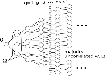
where hΔasubscriptsuperscript𝑎Δh^{a}_{\Delta} is termed as the “noise” part. Furthermore, we can assume that hΩsubscriptΩh_{\Omega} and hΔasubscriptsuperscript𝑎Δh^{a}_{\Delta} are asymptotically independent in the limit N𝑁N\to\infty. This assumption is reasonable, and a schematic to explain this is given in Fig. 1.
Refer to caption
Figure 1: Schematic explaining the independence between (s0,𝒔Ω)subscript𝑠0subscript𝒔Ω(s_{0},\bm{s}_{\Omega}) and hΔasubscriptsuperscript𝑎Δh^{a}_{\Delta}. The majority in the sum in hΔasuperscriptsubscriptΔ𝑎h_{\Delta}^{a} is uncorrelated with spins in ΩΩ\Omega and dominates hΔasubscriptsuperscript𝑎Δh^{a}_{\Delta} in the thermodynamic limit.

Owing to the tree-like structure, we can define the generation g𝑔g of a spin s𝑠s from ΩΩ\Omega as the shortest path length between s𝑠s and any spin in ΩΩ\Omega along the network. As g𝑔g grows, the correlation with {si|iΩ}conditional-setsubscript𝑠𝑖𝑖Ω\{s_{i}|i\in\Omega\} decays exponentially fast, while the number of spins belonging to generation g𝑔g exponentially increases. If the correlation decay is sufficiently faster than the increase of the spins, then the majority of spins in the network can be regarded as uncorrelated with ΩΩ\Omega. Some terms in hΔasubscriptsuperscript𝑎Δh^{a}_{\Delta} are certainly correlated with hsuperscripth^{*}, but their contribution is O(N1)𝑂superscript𝑁1O(\sqrt{N}^{-1}) because Δi=O(N1)subscriptΔ𝑖𝑂superscript𝑁1\Delta_{i}=O(\sqrt{N}^{-1}) and the number of correlating terms is O(1)𝑂1O(1) owing to the sufficiently fast decay of correlations. Hence, the contribution of correlating terms vanishes and the uncorrelated majority with ΩΩ\Omega completely dominates hΔasubscriptsuperscript𝑎Δh^{a}_{\Delta} in the thermodynamic limit. These observations indicate that eq. (17) can be now decomposed as follows:

[Zn]DM=Tr{𝑱a}a=1n{𝒔PIsing(𝒔|𝑱)eβa=1n(s0ha)}Msubscriptdelimited-[]superscript𝑍𝑛superscript𝐷𝑀subscriptTrsuperscriptsubscriptsuperscript𝑱𝑎𝑎1𝑛superscriptsubscript𝒔subscript𝑃Isingconditional𝒔superscript𝑱superscript𝑒𝛽superscriptsubscript𝑎1𝑛subscript𝑠0superscript𝑎𝑀\displaystyle\left[Z^{n}\right]_{D^{M}}=\mathop{\rm Tr}_{\{\bm{J}^{a}\}_{a=1}^{n}}\Biggl{\{}\sum_{\bm{s}}\int P_{\rm Ising}(\bm{s}\big{|}\bm{J}^{*})e^{-\beta\sum_{a=1}^{n}\ell\left(s_{0}h^{a}\right)}\Biggr{\}}^{M}
Tr{𝚫a}a=1n{𝒔a=1ndhΔaPIsing(𝒔|𝑱)δ(hΔajΩ¯Δjasj)eβa=1n(s0(jΩJ¯jsj+hΔa))}MabsentsubscriptTrsuperscriptsubscriptsuperscript𝚫𝑎𝑎1𝑛superscriptsubscript𝒔superscriptsubscriptproduct𝑎1𝑛𝑑subscriptsuperscript𝑎Δsubscript𝑃Isingconditional𝒔superscript𝑱𝛿subscriptsuperscript𝑎Δsubscript𝑗¯ΩsuperscriptsubscriptΔ𝑗𝑎subscript𝑠𝑗superscript𝑒𝛽superscriptsubscript𝑎1𝑛subscript𝑠0subscript𝑗Ωsubscript¯𝐽𝑗subscript𝑠𝑗superscriptsubscriptΔ𝑎𝑀\displaystyle\approx\mathop{\rm Tr}_{\{\bm{\Delta}^{a}\}_{a=1}^{n}}\Biggl{\{}\sum_{\bm{s}}\int\prod_{a=1}^{n}dh^{a}_{\Delta}P_{\rm Ising}(\bm{s}|\bm{J}^{*})\delta\left(h^{a}_{\Delta}-\sum_{j\in\bar{\Omega}}\Delta_{j}^{a}s_{j}\right)e^{-\beta\sum_{a=1}^{n}\ell\left(s_{0}\left(\sum_{j\in\Omega}\bar{J}_{j}s_{j}+h_{\Delta}^{a}\right)\right)}\Biggr{\}}^{M}
=Tr{𝚫a}a=1n{s0,𝒔Ωa=1ndhΔaP(s0,𝒔Ω,{hΔa}a|𝑱,{𝚫a}a)eβa=1n(s0(jΩJ¯jsj+hΔa))}MabsentsubscriptTrsuperscriptsubscriptsuperscript𝚫𝑎𝑎1𝑛superscriptsubscriptsubscript𝑠0subscript𝒔Ωsuperscriptsubscriptproduct𝑎1𝑛𝑑subscriptsuperscript𝑎Δ𝑃subscript𝑠0subscript𝒔Ωconditionalsubscriptsubscriptsuperscript𝑎Δ𝑎superscript𝑱subscriptsuperscript𝚫𝑎𝑎superscript𝑒𝛽superscriptsubscript𝑎1𝑛subscript𝑠0subscript𝑗Ωsubscript¯𝐽𝑗subscript𝑠𝑗superscriptsubscriptΔ𝑎𝑀\displaystyle=\mathop{\rm Tr}_{\{\bm{\Delta}^{a}\}_{a=1}^{n}}\Biggl{\{}\sum_{s_{0},\bm{s}_{\Omega}}\int\prod_{a=1}^{n}dh^{a}_{\Delta}P(s_{0},\bm{s}_{\Omega},\{h^{a}_{\Delta}\}_{a}|\bm{J}^{*},\{\bm{\Delta}^{a}\}_{a})e^{-\beta\sum_{a=1}^{n}\ell\left(s_{0}\left(\sum_{j\in\Omega}\bar{J}_{j}s_{j}+h_{\Delta}^{a}\right)\right)}\Biggr{\}}^{M}
Tr{𝚫a}a=1n{s0,𝒔Ωa=1ndhΔaPIsing(s0,𝒔Ω|𝑱)Pcav({hΔa}a|{𝚫a}a)\displaystyle\approx\mathop{\rm Tr}_{\{\bm{\Delta}^{a}\}_{a=1}^{n}}\Biggl{\{}\sum_{s_{0},\bm{s}_{\Omega}}\int\prod_{a=1}^{n}dh^{a}_{\Delta}P_{\rm Ising}(s_{0},\bm{s}_{\Omega}|\bm{J}^{*})P_{\rm cav}(\{h^{a}_{\Delta}\}_{a}|\{\bm{\Delta}^{a}\}_{a})
×eβa=1n(s0(jΩJ¯jsj+hΔa))}M.\displaystyle\times e^{-\beta\sum_{a=1}^{n}\ell\left(s_{0}\left(\sum_{j\in\Omega}\bar{J}_{j}s_{j}+h_{\Delta}^{a}\right)\right)}\Biggr{\}}^{M}. (42)

In the second line, we performed the variable transformation 𝚫a=𝑱a𝑱¯superscript𝚫𝑎superscript𝑱𝑎¯𝑱\bm{\Delta}^{a}=\bm{J}^{a}-\bar{\bm{J}} and neglected the contribution jΩΔjasjsubscript𝑗ΩsuperscriptsubscriptΔ𝑗𝑎subscript𝑠𝑗\sum_{j\in\Omega}\Delta_{j}^{a}s_{j} in hΔasubscriptsuperscript𝑎Δh^{a}_{\Delta} as eq. (41). In the third line, we denoted 𝒔Ω={si|iΩ}subscript𝒔Ωconditional-setsubscript𝑠𝑖𝑖Ω\bm{s}_{\Omega}=\{s_{i}|i\in\Omega\} and 𝒔Ω¯={si|iΩ¯}subscript𝒔¯Ωconditional-setsubscript𝑠𝑖𝑖¯Ω\bm{s}_{\bar{\Omega}}=\{s_{i}|i\in\bar{\Omega}\}, and performed the sum over 𝒔Ω¯subscript𝒔¯Ω\bm{s}_{\bar{\Omega}}, yielding the joint distribution P(s0,𝒔Ω,{hΔa}a|𝑱,{𝚫a}a)𝑃subscript𝑠0subscript𝒔Ωconditionalsubscriptsubscriptsuperscript𝑎Δ𝑎superscript𝑱subscriptsuperscript𝚫𝑎𝑎P(s_{0},\bm{s}_{\Omega},\{h^{a}_{\Delta}\}_{a}|\bm{J}^{*},\{\bm{\Delta}^{a}\}_{a}). In the fourth line, we used the asymptotic uncorrelatedness between hΔasuperscriptsubscriptΔ𝑎h_{\Delta}^{a} and (s0,𝒔Ω)subscript𝑠0subscript𝒔Ω(s_{0},\bm{s}_{\Omega}) discussed so far.

Now, the central limit theorem can be applied to the noise part {hΔa}asubscriptsubscriptsuperscript𝑎Δ𝑎\{h^{a}_{\Delta}\}_{a}, and they can be regarded as Gaussian variables. As the fully-connected case, two order parameters describing their covariances are introduced:

Qi,jCij\0ΔiaΔja,𝑄subscript𝑖𝑗superscriptsubscript𝐶𝑖𝑗\absent0superscriptsubscriptΔ𝑖𝑎superscriptsubscriptΔ𝑗𝑎\displaystyle Q\equiv\sum_{i,j}C_{ij}^{\backslash 0}\Delta_{i}^{a}\Delta_{j}^{a}, (43)
qi,jCij\0ΔiaΔjb,(ab).𝑞subscript𝑖𝑗superscriptsubscript𝐶𝑖𝑗\absent0superscriptsubscriptΔ𝑖𝑎superscriptsubscriptΔ𝑗𝑏𝑎𝑏\displaystyle q\equiv\sum_{i,j}C_{ij}^{\backslash 0}\Delta_{i}^{a}\Delta_{j}^{b},~{}(a\neq b). (44)

Counterparts of m𝑚m and Qsuperscript𝑄Q^{*} are unnecessary because the dependence on (s0,𝒔Ω)subscript𝑠0subscript𝒔Ω(s_{0},\bm{s}_{\Omega}) is separately and explicitly treated in the present formulation. Then,

[Zn]DM𝑑Q𝑑qeNS(C\0,Q,q)+MlogL(𝑱,𝑱¯,Q,q),subscriptdelimited-[]superscript𝑍𝑛superscript𝐷𝑀differential-d𝑄differential-d𝑞superscript𝑒𝑁𝑆superscript𝐶\absent0𝑄𝑞𝑀𝐿superscript𝑱¯𝑱𝑄𝑞\displaystyle\left[Z^{n}\right]_{D^{M}}\approx\int dQdq~{}e^{NS\left(C^{\backslash 0},Q,q\right)+M\log L(\bm{J}^{*},\bar{\bm{J}},Q,q)}, (45)

where

eNS(C\0,Q,q)Tr{𝚫a}a=1na=1nδ(Qi,jCij\0ΔiaΔja)a<bδ(qi,jCij\0ΔiaΔjb),superscript𝑒𝑁𝑆superscript𝐶\absent0𝑄𝑞subscriptTrsuperscriptsubscriptsuperscript𝚫𝑎𝑎1𝑛superscriptsubscriptproduct𝑎1𝑛𝛿𝑄subscript𝑖𝑗superscriptsubscript𝐶𝑖𝑗\absent0superscriptsubscriptΔ𝑖𝑎superscriptsubscriptΔ𝑗𝑎subscriptproduct𝑎𝑏𝛿𝑞subscript𝑖𝑗superscriptsubscript𝐶𝑖𝑗\absent0superscriptsubscriptΔ𝑖𝑎superscriptsubscriptΔ𝑗𝑏\displaystyle e^{NS\left(C^{\backslash 0},Q,q\right)}\equiv\mathop{\rm Tr}_{\{\bm{\Delta}^{a}\}_{a=1}^{n}}\prod_{a=1}^{n}\delta\left(Q-\sum_{i,j}C_{ij}^{\backslash 0}\Delta_{i}^{a}\Delta_{j}^{a}\right)\prod_{a<b}\delta\left(q-\sum_{i,j}C_{ij}^{\backslash 0}\Delta_{i}^{a}\Delta_{j}^{b}\right), (46)
L(𝑱,𝑱¯,Q,q)=s0,𝒔Ωa=1ndhΔaPIsing(s0,𝒔Ω|𝑱)Pcav({hΔa}a=1n|Q,q)𝐿superscript𝑱¯𝑱𝑄𝑞subscriptsubscript𝑠0subscript𝒔Ωsuperscriptsubscriptproduct𝑎1𝑛𝑑subscriptsuperscript𝑎Δsubscript𝑃Isingsubscript𝑠0conditionalsubscript𝒔Ωsuperscript𝑱subscript𝑃cavconditionalsuperscriptsubscriptsubscriptsuperscript𝑎Δ𝑎1𝑛𝑄𝑞\displaystyle L(\bm{J}^{*},\bar{\bm{J}},Q,q)=\sum_{s_{0},\bm{s}_{\Omega}}\int\prod_{a=1}^{n}dh^{a}_{\Delta}P_{\rm Ising}(s_{0},\bm{s}_{\Omega}|\bm{J}^{*})P_{\rm cav}(\left\{h^{a}_{\Delta}\right\}_{a=1}^{n}\big{|}Q,q)
×eβa=1n(s0(jΩJ¯jsj+hΔa)).absentsuperscript𝑒𝛽superscriptsubscript𝑎1𝑛subscript𝑠0subscript𝑗Ωsubscript¯𝐽𝑗subscript𝑠𝑗subscriptsuperscript𝑎Δ\displaystyle\times e^{-\beta\sum_{a=1}^{n}\ell\left(s_{0}\left(\sum_{j\in\Omega}\bar{J}_{j}s_{j}+h^{a}_{\Delta}\right)\right)}. (47)

Again, using the techniques in sec. A we get

limn01nS(C\0,Q,q)=12{QQq+log2π+log(Qq)1NTrlogC\0},subscript𝑛01𝑛𝑆superscript𝐶\absent0𝑄𝑞12𝑄𝑄𝑞2𝜋𝑄𝑞1𝑁Trsuperscript𝐶\absent0\displaystyle\lim_{n\to 0}\frac{1}{n}S\left(C^{\backslash 0},Q,q\right)=\frac{1}{2}\left\{\frac{Q}{Q-q}+\log 2\pi+\log(Q-q)-\frac{1}{N}\mathop{\rm Tr}\log C^{\backslash 0}\right\}, (48)
limn01nlogL(𝑱,𝑱¯,Q,q)=s0,𝒔ΩPIsing(s0,𝒔Ω|𝑱)subscript𝑛01𝑛𝐿superscript𝑱¯𝑱𝑄𝑞subscriptsubscript𝑠0subscript𝒔Ωsubscript𝑃Isingsubscript𝑠0conditionalsubscript𝒔Ωsuperscript𝑱\displaystyle\lim_{n\to 0}\frac{1}{n}\log L\left(\bm{J}^{*},\bar{\bm{J}},Q,q\right)=\sum_{s_{0},\bm{s}_{\Omega}}P_{\rm Ising}(s_{0},\bm{s}_{\Omega}|\bm{J}^{*})
×DzlogDveβ(s0(jΩJ¯jsj+Qqv+qz)).\displaystyle\times\int Dz\log\int Dv~{}e^{-\beta\ell\left(s_{0}\left(\sum_{j\in\Omega}\bar{J}_{j}s_{j}+\sqrt{Q-q}v+\sqrt{q}z\right)\right)}. (49)

Employing the relation (28) and taking the β𝛽\beta\to\infty limit, we get

fave=ExtrQ,χ{12Qχ\displaystyle f^{\rm ave}=-\mathop{\rm Extr}_{Q,\chi}\Bigg{\{}\frac{1}{2}\frac{Q}{\chi}
+αs0,𝒔ΩPIsing(s0,𝒔Ω|𝑱)Dzmaxy((ys0(Qz+jΩJ¯jsj))22χ(y))}.\displaystyle+\alpha\sum_{s_{0},\bm{s}_{\Omega}}P_{\rm Ising}(s_{0},\bm{s}_{\Omega}|\bm{J}^{*})\int Dz\max_{y}\left(-\frac{\left(y-s_{0}(\sqrt{Q}z+\sum_{j\in\Omega}\bar{J}_{j}s_{j})\right)^{2}}{2\chi}-\ell\left(y\right)\right)\Bigg{\}}. (50)

The extremization condition with respect to Q𝑄Q and χ𝜒\chi gives

0=1χαQs0,𝒔ΩPIsing(s0,𝒔Ω|𝑱)s0Dzzy|y=y^,01𝜒evaluated-at𝛼𝑄subscriptsubscript𝑠0subscript𝒔Ωsubscript𝑃Isingsubscript𝑠0conditionalsubscript𝒔Ωsuperscript𝑱subscript𝑠0𝐷𝑧𝑧𝑦𝑦^𝑦\displaystyle 0=\frac{1}{\chi}-\frac{\alpha}{\sqrt{Q}}\sum_{s_{0},\bm{s}_{\Omega}}P_{\rm Ising}(s_{0},\bm{s}_{\Omega}|\bm{J}^{*})s_{0}\int Dzz\frac{\partial\ell}{\partial y}\Bigg{|}_{y=\hat{y}}, (51a)
0=Qχ2+αs0,𝒔ΩPIsing(s0,𝒔Ω|𝑱)Dz(y|y=y^)2,0𝑄superscript𝜒2𝛼subscriptsubscript𝑠0subscript𝒔Ωsubscript𝑃Isingsubscript𝑠0conditionalsubscript𝒔Ωsuperscript𝑱𝐷𝑧superscriptevaluated-at𝑦𝑦^𝑦2\displaystyle 0=-\frac{Q}{\chi^{2}}+\alpha\sum_{s_{0},\bm{s}_{\Omega}}P_{\rm Ising}(s_{0},\bm{s}_{\Omega}|\bm{J}^{*})\int Dz\left(\frac{\partial\ell}{\partial y}\Bigg{|}_{y=\hat{y}}\right)^{2}, (51b)

where

y^(z,s0,𝒔Ω|Q,χ,{J¯j}jΩ)=argmaxy((ys0(Qz+jΩJ¯jsj))22χ(y)).^𝑦𝑧subscript𝑠0conditionalsubscript𝒔Ω𝑄𝜒subscriptsubscript¯𝐽𝑗𝑗Ωsubscriptargmax𝑦superscript𝑦subscript𝑠0𝑄𝑧subscript𝑗Ωsubscript¯𝐽𝑗subscript𝑠𝑗22𝜒𝑦\displaystyle\hat{y}(z,s_{0},\bm{s}_{\Omega}|Q,\chi,\{\bar{J}_{j}\}_{j\in\Omega})=\operatorname*{arg\,max}_{y}\left(-\frac{\left(y-s_{0}\left(\sqrt{Q}z+\sum_{j\in\Omega}\bar{J}_{j}s_{j}\right)\right)^{2}}{2\chi}-\ell(y)\right). (52)

Further, the mean estimates {J¯j}jΩsubscriptsubscript¯𝐽𝑗𝑗Ω\{\bar{J}_{j}\}_{j\in\Omega} are also evaluated by the extremization condition. The result for J¯jsubscript¯𝐽𝑗\bar{J}_{j} is given by

0=s0,𝒔ΩPIsing(s0,𝒔Ω|𝑱)Dzy|y=y^s0sj.0evaluated-atsubscriptsubscript𝑠0subscript𝒔Ωsubscript𝑃Isingsubscript𝑠0conditionalsubscript𝒔Ωsuperscript𝑱𝐷𝑧𝑦𝑦^𝑦subscript𝑠0subscript𝑠𝑗\displaystyle 0=\sum_{s_{0},\bm{s}_{\Omega}}P_{\rm Ising}(s_{0},\bm{s}_{\Omega}|\bm{J}^{*})\int Dz\frac{\partial\ell}{\partial y}\Bigg{|}_{y=\hat{y}}s_{0}s_{j}. (53)

Using the parameters Q,χ,{J¯i}iΩ𝑄𝜒subscriptsubscript¯𝐽𝑖𝑖ΩQ,\chi,\{\bar{J}_{i}\}_{i\in\Omega} computed by eqs. (51-53), we can evaluate the RSS which is expressed in the present setting as

iΩ(JiJ¯i)2+iΩ¯Δi2=iΩ(JiJ¯i)2+QNTr(C\0)1.subscript𝑖Ωsuperscriptsuperscriptsubscript𝐽𝑖subscript¯𝐽𝑖2subscript𝑖¯ΩsuperscriptsubscriptΔ𝑖2subscript𝑖Ωsuperscriptsuperscriptsubscript𝐽𝑖subscript¯𝐽𝑖2𝑄𝑁Trsuperscriptsuperscript𝐶\absent01\displaystyle\mathcal{E}\approx\sum_{i\in\Omega}(J_{i}^{*}-\bar{J}_{i})^{2}+\sum_{i\in\bar{\Omega}}{\Delta}_{i}^{2}=\sum_{i\in\Omega}(J_{i}^{*}-\bar{J}_{i})^{2}+\frac{Q}{N}\mathop{\rm Tr}\left(C^{\backslash 0}\right)^{-1}. (54)

The quantity (C\0)1superscriptsuperscript𝐶\absent01\left(C^{\backslash 0}\right)^{-1} will be computed in another discussion on the direct problem as the fully-connected case. In addition, PIsing(s0,𝒔Ω|𝑱)subscript𝑃Isingsubscript𝑠0conditionalsubscript𝒔Ωsuperscript𝑱P_{\rm Ising}(s_{0},\bm{s}_{\Omega}|\bm{J}^{*}) will also be assessed separately in the sparse case. These points are addressed in the next subsection.

3.2 Direct problem’s properties

The inverse problem essentially requires certain information from its direct problem counterpart. Necessary information to compute the quantities of interest depends on the system’s properties. In the fully-connected case, two-body quantities such as (C\0)1superscriptsuperscript𝐶\absent01\left(C^{\backslash 0}\right)^{-1} and i,jCij\0JiJjsubscript𝑖𝑗subscriptsuperscript𝐶\absent0𝑖𝑗superscriptsubscript𝐽𝑖superscriptsubscript𝐽𝑗\sum_{i,j}C^{\backslash 0}_{ij}J_{i}^{*}J_{j}^{*} are sufficient. However, in the sparse case, higher-order information is needed because the central limit theorem does not fully dominate the system. Hence, the functional form of PIsing(s0,𝒔Ω)subscript𝑃Isingsubscript𝑠0subscript𝒔ΩP_{\rm Ising}(s_{0},\bm{s}_{\Omega}) becomes necessary, as seen in eq. (50). Techniques for computing such quantities in the sparse case largely advanced in the ’90–’00s. Here, we quote a portion of the results to compute the necessary quantities. For readers interested in the detailed techniques, please refer to [31, 32]. Although these techniques are applied in general situations, to obtain compact analytic forms of the quantities of interest, we rely on the assumptions that the teacher model is in the paramagnetic phase and the external fields are absent.

3.2.1 Marginal distribution of the teacher model

The marginal distribution PIsing(s0,𝒔Ω|𝑱)subscript𝑃Isingsubscript𝑠0conditionalsubscript𝒔Ωsuperscript𝑱P_{\rm Ising}(s_{0},\bm{s}_{\Omega}|\bm{J}^{*}) is computed by marginalizing the whole distribution PIsing(𝒔|𝑱)subscript𝑃Isingconditional𝒔superscript𝑱P_{\rm Ising}(\bm{s}|\bm{J}^{*}) with respect to 𝒔Ω¯subscript𝒔¯Ω\bm{s}_{\bar{\Omega}}. In general, this operation requires nontrivial computations and the resultant distribution becomes dependent on parameters among the marginalized spins. However, under the present assumptions, such dependencies do not exist and the expression becomes rather simple:

PIsing(s0,𝒔Ω|𝑱)=1ZΩces0jΩJjsj,ZΩc=s0,𝒔Ωes0jΩJjsj,formulae-sequencesubscript𝑃Isingsubscript𝑠0conditionalsubscript𝒔Ωsuperscript𝑱1subscript𝑍subscriptΩ𝑐superscript𝑒subscript𝑠0subscript𝑗Ωsuperscriptsubscript𝐽𝑗subscript𝑠𝑗subscript𝑍subscriptΩ𝑐subscriptsubscript𝑠0subscript𝒔Ωsuperscript𝑒subscript𝑠0subscript𝑗Ωsuperscriptsubscript𝐽𝑗subscript𝑠𝑗\displaystyle P_{\rm Ising}(s_{0},\bm{s}_{\Omega}|\bm{J}^{*})=\frac{1}{Z_{\Omega_{c}}}e^{s_{0}\sum_{j\in\Omega}J_{j}^{*}s_{j}},~{}Z_{\Omega_{c}}=\sum_{s_{0},\bm{s}_{\Omega}}e^{s_{0}\sum_{j\in\Omega}J_{j}^{*}s_{j}}, (55)

where ΩcsubscriptΩ𝑐\Omega_{c} denotes the union index set of 00 and ΩΩ\Omega. This form is applied to eqs. (51,53) to obtain the order parameters.

3.2.2 Inverse correlation function

Next, we compute the inverse correlation function C1superscript𝐶1C^{-1}; hereafter, we treat the whole system and discard the superscript \0 as it is not essential.

On the tree-like networks, the so-called Bethe approximation gives an exact result as the system size tends to infinity, and it provide a compact analytic form of the inverse correlation function. The derivation is given in [33, 34] and we here just quote the result. Under the present assumptions without magnetizations and external fields, it becomes

(C1)ij=(ki11tanh2(Jik)(ci1))δijtanh(Jij)1tanh2(Jij)(1δij),subscriptsuperscript𝐶1𝑖𝑗subscript𝑘𝑖11superscript2subscript𝐽𝑖𝑘subscript𝑐𝑖1subscript𝛿𝑖𝑗subscript𝐽𝑖𝑗1superscript2subscript𝐽𝑖𝑗1subscript𝛿𝑖𝑗\displaystyle\left(C^{-1}\right)_{ij}=\left(\sum_{k\in\partial i}\frac{1}{1-\tanh^{2}(J_{ik})}-(c_{i}-1)\right)\delta_{ij}-\frac{\tanh(J_{ij})}{1-\tanh^{2}(J_{ij})}(1-\delta_{ij}), (56)

where i𝑖\partial i denotes the index set of nodes connected to i𝑖i and cisubscript𝑐𝑖c_{i} denotes the connectivity or the number of edges connecting to node i𝑖i.

3.3 Applicable range of the ansatz

Here we consider the applicable range of the ansatz (38). This ansatz is a strong statement since it allows us to not think of any possible biases of the estimators outside the active set ΩΩ\Omega. When is this valid? How does it relate to the tree-like network structure?

To obtain answers to these questions, we rethink eq. (53). An important observation is that this equation is merely the zero-gradient condition of \ell with respect to Jj,(jΩ)subscript𝐽𝑗𝑗ΩJ_{j},(j\in\Omega) averaged over the datasets, as shown below. Denoting the empirical average on the dataset DMsuperscript𝐷𝑀D^{M} by ¯DMsuperscript¯superscript𝐷𝑀\overline{\cdots}^{D^{M}}, and using the statistical mechanical analysis explained so far, we can write the zero-gradient condition with respect to Jjsubscript𝐽𝑗J_{j} for jΩ𝑗Ωj\in\Omega as

0=(s0h(𝒔\0,𝑱))Jj|𝑱=𝑱^(DM)¯DM=(y)ys0sj¯DM,0superscript¯evaluated-atsubscript𝑠0subscript𝒔\absent0𝑱subscript𝐽𝑗𝑱^𝑱superscript𝐷𝑀superscript𝐷𝑀superscript¯𝑦𝑦subscript𝑠0subscript𝑠𝑗superscript𝐷𝑀\displaystyle 0=\overline{\frac{\partial\ell(s_{0}h(\bm{s}_{\backslash 0},\bm{J}))}{\partial J_{j}}\Biggr{|}_{\bm{J}=\hat{\bm{J}}(D^{M})}}^{D^{M}}=\overline{\frac{\partial\ell(y)}{\partial y}s_{0}s_{j}}^{D^{M}}, (57)

where we put y=s0h(𝒔\0,𝑱^)=s0(iJ^isi)𝑦subscript𝑠0subscript𝒔\absent0^𝑱subscript𝑠0subscript𝑖subscript^𝐽𝑖subscript𝑠𝑖y=s_{0}h(\bm{s}_{\backslash 0},\hat{\bm{J}})=s_{0}\left(\sum_{i}\hat{J}_{i}s_{i}\right). With this expression, we replace the estimator 𝑱^^𝑱\hat{\bm{J}} with the average over eq. (11), take the average over the dataset, and use the replica method. The result is

0=limβlimn0Tr{𝑱a}a=1n(𝒔PIsing(𝒔|𝑱)eβa=1n(ya))M10subscript𝛽subscript𝑛0subscriptTrsuperscriptsubscriptsuperscript𝑱𝑎𝑎1𝑛superscriptsubscript𝒔subscript𝑃Isingconditional𝒔superscript𝑱superscript𝑒𝛽superscriptsubscript𝑎1𝑛superscript𝑦𝑎𝑀1\displaystyle 0=\lim_{\beta\to\infty}\lim_{n\to 0}\mathop{\rm Tr}_{\{\bm{J}^{a}\}_{a=1}^{n}}\left(\sum_{\bm{s}}P_{\rm Ising}(\bm{s}\big{|}\bm{J}^{*})e^{-\beta\sum_{a=1}^{n}\ell(y^{a})}\right)^{M-1}
×(𝒔PIsing(𝒔|𝑱)eβa=1n(ya)(y1)y1s0sj).absentsubscript𝒔subscript𝑃Isingconditional𝒔superscript𝑱superscript𝑒𝛽superscriptsubscript𝑎1𝑛superscript𝑦𝑎superscript𝑦1superscript𝑦1subscript𝑠0subscript𝑠𝑗\displaystyle\times\left(\sum_{\bm{s}}P_{\rm Ising}(\bm{s}\big{|}\bm{J}^{*})e^{-\beta\sum_{a=1}^{n}\ell(y^{a})}\frac{\partial\ell(y^{1})}{\partial y^{1}}s_{0}s_{j}\right). (58)

where yas0(iJiasj)superscript𝑦𝑎subscript𝑠0subscript𝑖superscriptsubscript𝐽𝑖𝑎subscript𝑠𝑗y^{a}\equiv s_{0}\left(\sum_{i}J_{i}^{a}s_{j}\right). The ansatz (38) and RS used in sec. 3.1, in short, say

ya=ansatzs0{iΩJ¯isi+hΔa}=RSs0{iΩJ¯isi+Qqva+qz}.superscript𝑦𝑎ansatzsubscript𝑠0subscript𝑖Ωsubscript¯𝐽𝑖subscript𝑠𝑖superscriptsubscriptΔ𝑎RSsubscript𝑠0subscript𝑖Ωsubscript¯𝐽𝑖subscript𝑠𝑖𝑄𝑞superscript𝑣𝑎𝑞𝑧\displaystyle y^{a}\overset{\mathrm{ansatz}}{=}s_{0}\left\{\sum_{i\in\Omega}\bar{J}_{i}s_{i}+h_{\Delta}^{a}\right\}\overset{\mathrm{RS}}{=}s_{0}\left\{\sum_{i\in\Omega}\bar{J}_{i}s_{i}+\sqrt{Q-q}v^{a}+\sqrt{q}z\right\}. (59)

where va,z𝒩(0,1)similar-tosuperscript𝑣𝑎𝑧𝒩01v^{a},z\sim\mathcal{N}(0,1). Applying this form and following the same line of computations as in sec. 3.1, we get

(𝒔PIsing(𝒔|𝑱)eβa=1n(ya)(y1)y1s0sj)subscript𝒔subscript𝑃Isingconditional𝒔superscript𝑱superscript𝑒𝛽superscriptsubscript𝑎1𝑛superscript𝑦𝑎superscript𝑦1superscript𝑦1subscript𝑠0subscript𝑠𝑗\displaystyle\left(\sum_{\bm{s}}P_{\rm Ising}(\bm{s}\big{|}\bm{J}^{*})e^{-\beta\sum_{a=1}^{n}\ell(y^{a})}\frac{\partial\ell(y^{1})}{\partial y^{1}}s_{0}s_{j}\right)
Ns0,𝒔ΩPIsing(s0,𝒔Ω|𝑱)Dz(Dveβ(y(z,v)))nDv1eβ(y(z,v1))(y1)y1s0sjDv1eβ(y(z,v1))𝑁subscriptsubscript𝑠0subscript𝒔Ωsubscript𝑃Isingsubscript𝑠0conditionalsubscript𝒔Ωsuperscript𝑱𝐷𝑧superscript𝐷𝑣superscript𝑒𝛽𝑦𝑧𝑣𝑛𝐷superscript𝑣1superscript𝑒𝛽𝑦𝑧superscript𝑣1superscript𝑦1superscript𝑦1subscript𝑠0subscript𝑠𝑗𝐷superscript𝑣1superscript𝑒𝛽𝑦𝑧superscript𝑣1\displaystyle\overset{N\to\infty}{\longrightarrow}\sum_{s_{0},\bm{s}_{\Omega}}P_{\rm Ising}(s_{0},\bm{s}_{\Omega}\big{|}\bm{J}^{*})\int Dz\left(\int Dve^{-\beta\ell(y(z,v))}\right)^{n}\frac{\int Dv^{1}e^{-\beta\ell(y(z,v^{1}))}\frac{\partial\ell(y^{1})}{\partial y^{1}}s_{0}s_{j}}{\int Dv^{1}e^{-\beta\ell(y(z,v^{1}))}}
n0s0,𝒔ΩPIsing(s0,𝒔Ω|𝑱)DzDveβ(y(z,v))(y)ys0sjDveβ(y(z,v))𝑛0subscriptsubscript𝑠0subscript𝒔Ωsubscript𝑃Isingsubscript𝑠0conditionalsubscript𝒔Ωsuperscript𝑱𝐷𝑧𝐷𝑣superscript𝑒𝛽𝑦𝑧𝑣𝑦𝑦subscript𝑠0subscript𝑠𝑗𝐷𝑣superscript𝑒𝛽𝑦𝑧𝑣\displaystyle\overset{n\to 0}{\longrightarrow}\sum_{s_{0},\bm{s}_{\Omega}}P_{\rm Ising}(s_{0},\bm{s}_{\Omega}\big{|}\bm{J}^{*})\int Dz\frac{\int Dve^{-\beta\ell(y(z,v))}\frac{\partial\ell(y)}{\partial y}s_{0}s_{j}}{\int Dve^{-\beta\ell(y(z,v))}}
βs0,𝒔ΩPIsing(s0,𝒔Ω|𝑱)Dz(y)y|y=y^s0sj,evaluated-at𝛽subscriptsubscript𝑠0subscript𝒔Ωsubscript𝑃Isingsubscript𝑠0conditionalsubscript𝒔Ωsuperscript𝑱𝐷𝑧𝑦𝑦𝑦^𝑦subscript𝑠0subscript𝑠𝑗\displaystyle\overset{\beta\to\infty}{\longrightarrow}\sum_{s_{0},\bm{s}_{\Omega}}P_{\rm Ising}(s_{0},\bm{s}_{\Omega}\big{|}\bm{J}^{*})\int Dz\frac{\partial\ell(y)}{\partial y}\Biggr{|}_{y=\hat{y}}s_{0}s_{j}, (60)

and the factor (𝒔PIsing(𝒔|𝑱)eβa=1n(ya))M1superscriptsubscript𝒔subscript𝑃Isingconditional𝒔superscript𝑱superscript𝑒𝛽superscriptsubscript𝑎1𝑛superscript𝑦𝑎𝑀1\left(\sum_{\bm{s}}P_{\rm Ising}(\bm{s}\big{|}\bm{J}^{*})e^{-\beta\sum_{a=1}^{n}\ell(y^{a})}\right)^{M-1} in eq. (58) becomes unity when taking the n0𝑛0n\to 0 limit, yielding the identical result to eq. (53).

This computation naturally leads to the following question: Should we compute all the zero-gradient conditions not only for ΩΩ\Omega but also for Ω¯¯Ω\bar{\Omega}? This point is important because if this is the case, then the ansatz (38) is insufficient as it only suffices those for the active set jΩ𝑗Ωj\in\Omega. To be consistent, the answer is considered to be yes in general; hence, we need to take into account the zero-gradient conditions for kΩ¯𝑘¯Ωk\in\bar{\Omega}. This implies that the ansatz (38) should be modified and we need to introduce mean estimates J¯ksubscript¯𝐽𝑘\bar{J}_{k} for kΩ¯𝑘¯Ωk\in\bar{\Omega} in general situations.

Fortunately, if the network is tree-like, we can show that all the zero-gradient conditions are automatically satisfied once those for jΩfor-all𝑗Ω\forall j\in\Omega are met. Hence, the ansatz (38) is consistent on such networks; we show proof of this below. For technical reasons, we recover the external field 𝑯superscript𝑯\bm{H}^{*} in the remaining of this subsection. When the external field exists, the student model should also have the external field variable, and hence the replica result is slightly modified. That modification is accomplished by replacing (jΩJ¯jsj)subscript𝑗Ωsubscript¯𝐽𝑗subscript𝑠𝑗\left(\sum_{j\in\Omega}\bar{J}_{j}s_{j}\right) with (jΩJ¯jsj+H¯0)subscript𝑗Ωsubscript¯𝐽𝑗subscript𝑠𝑗subscript¯𝐻0\left(\sum_{j\in\Omega}\bar{J}_{j}s_{j}+\bar{H}_{0}\right) in eqs. (50,52) and (59). Here, H¯0subscript¯𝐻0\bar{H}_{0} denotes the mean estimate of the external field variable acting on the focused spin s0subscript𝑠0s_{0} of the student model, and is determined by the extremization condition of the free energy, yielding

0=s0,𝒔ΩPIsing(s0,𝒔Ω|𝑱,𝑯)Dzy|y=y^s0.0evaluated-atsubscriptsubscript𝑠0subscript𝒔Ωsubscript𝑃Isingsubscript𝑠0conditionalsubscript𝒔Ωsuperscript𝑱superscript𝑯𝐷𝑧𝑦𝑦^𝑦subscript𝑠0\displaystyle 0=\sum_{s_{0},\bm{s}_{\Omega}}P_{\rm Ising}(s_{0},\bm{s}_{\Omega}|\bm{J}^{*},\bm{H}^{*})\int Dz\frac{\partial\ell}{\partial y}\Bigg{|}_{y=\hat{y}}s_{0}. (61)

Under the above setup, we show the consistency of eq. (38) on tree-like networks. The first step is to write down the zero-gradient condition for kΩ¯𝑘¯Ωk\in\bar{\Omega}. The result of applying the averages and replica method is the replacement of sjsubscript𝑠𝑗s_{j} with sksubscript𝑠𝑘s_{k} in eq. (58). With this expression, we perform the following transformation:

𝒔PIsing(𝒔|𝑱,𝑯)eβa=1n(ya)(y1)y1s0sk=Hk(𝒔PIsing(𝒔|𝑱,𝑯)eβa=1n(ya)(y1)y1s0)subscript𝒔subscript𝑃Isingconditional𝒔superscript𝑱superscript𝑯superscript𝑒𝛽superscriptsubscript𝑎1𝑛superscript𝑦𝑎superscript𝑦1superscript𝑦1subscript𝑠0subscript𝑠𝑘superscriptsubscript𝐻𝑘subscript𝒔subscript𝑃Isingconditional𝒔superscript𝑱superscript𝑯superscript𝑒𝛽superscriptsubscript𝑎1𝑛superscript𝑦𝑎superscript𝑦1superscript𝑦1subscript𝑠0\displaystyle\sum_{\bm{s}}P_{\rm Ising}(\bm{s}\big{|}\bm{J}^{*},\bm{H}^{*})e^{-\beta\sum_{a=1}^{n}\ell(y^{a})}\frac{\partial\ell(y^{1})}{\partial y^{1}}s_{0}s_{k}=\frac{\partial}{\partial H_{k}^{*}}\left(\sum_{\bm{s}}P_{\rm Ising}(\bm{s}\big{|}\bm{J}^{*},\bm{H}^{*})e^{-\beta\sum_{a=1}^{n}\ell(y^{a})}\frac{\partial\ell(y^{1})}{\partial y^{1}}s_{0}\right)
+(𝒔PIsing(𝒔|𝑱,𝑯)eβa=1n(ya)(y1)y1s0)sk,subscript𝒔subscript𝑃Isingconditional𝒔superscript𝑱superscript𝑯superscript𝑒𝛽superscriptsubscript𝑎1𝑛superscript𝑦𝑎superscript𝑦1superscript𝑦1subscript𝑠0delimited-⟨⟩subscript𝑠𝑘\displaystyle+\left(\sum_{\bm{s}}P_{\rm Ising}(\bm{s}\big{|}\bm{J}^{*},\bm{H}^{*})e^{-\beta\sum_{a=1}^{n}\ell(y^{a})}\frac{\partial\ell(y^{1})}{\partial y^{1}}s_{0}\right)\left\langle{s_{k}}\right\rangle, (62)

where delimited-⟨⟩\left\langle{\cdots}\right\rangle denotes the average over PIsing(𝒔|𝑱,𝑯)subscript𝑃Isingconditional𝒔superscript𝑱superscript𝑯P_{\rm Ising}(\bm{s}\big{|}\bm{J}^{*},\bm{H}^{*}). By following the same computations so far, the second term vanishes in the limit limβlimn0limNsubscript𝛽subscript𝑛0subscript𝑁\lim_{\beta\to\infty}\lim_{n\to 0}\lim_{N\to\infty} because the coefficient converges to the right-hand side of (61) giving zero. Meanwhile, in the same limit, the first term can be transformed as

Hk(𝒔PIsing(𝒔|𝑱,𝑯)eβa=1n(ya)(y1)y1s0)superscriptsubscript𝐻𝑘subscript𝒔subscript𝑃Isingconditional𝒔superscript𝑱superscript𝑯superscript𝑒𝛽superscriptsubscript𝑎1𝑛superscript𝑦𝑎superscript𝑦1superscript𝑦1subscript𝑠0\displaystyle\frac{\partial}{\partial H_{k}^{*}}\left(\sum_{\bm{s}}P_{\rm Ising}(\bm{s}\big{|}\bm{J}^{*},\bm{H}^{*})e^{-\beta\sum_{a=1}^{n}\ell(y^{a})}\frac{\partial\ell(y^{1})}{\partial y^{1}}s_{0}\right)
Hk(s0,𝒔ΩPIsing(s0,𝒔Ω|𝑱,𝑯)Dz(y)y|y=y^s0),absentsuperscriptsubscript𝐻𝑘evaluated-atsubscriptsubscript𝑠0subscript𝒔Ωsubscript𝑃Isingsubscript𝑠0conditionalsubscript𝒔Ωsuperscript𝑱superscript𝑯𝐷𝑧𝑦𝑦𝑦^𝑦subscript𝑠0\displaystyle\to\frac{\partial}{\partial H_{k}^{*}}\left(\sum_{s_{0},\bm{s}_{\Omega}}P_{\rm Ising}(s_{0},\bm{s}_{\Omega}\big{|}\bm{J}^{*},\bm{H}^{*})\int Dz\frac{\partial\ell(y)}{\partial y}\Biggr{|}_{y=\hat{y}}s_{0}\right), (63)

and the dependence on Hksuperscriptsubscript𝐻𝑘H_{k}^{*} appears only in the marginal distribution PIsing(s0,𝒔Ω|𝑱,𝑯)subscript𝑃Isingsubscript𝑠0conditionalsubscript𝒔Ωsuperscript𝑱superscript𝑯P_{\rm Ising}(s_{0},\bm{s}_{\Omega}\big{|}\bm{J}^{*},\bm{H}^{*}). On tree-like networks, the marginal distribution necessarily takes the following form:

PIsing(s0,𝒔Ω|𝑱,𝑯)=1Zes0(iΩJisi+H0)+iΩhi\0si,subscript𝑃Isingsubscript𝑠0conditionalsubscript𝒔Ωsuperscript𝑱superscript𝑯1𝑍superscript𝑒subscript𝑠0subscript𝑖Ωsuperscriptsubscript𝐽𝑖subscript𝑠𝑖superscriptsubscript𝐻0subscript𝑖Ωsuperscriptsubscript𝑖\absent0subscript𝑠𝑖\displaystyle P_{\rm Ising}(s_{0},\bm{s}_{\Omega}\big{|}\bm{J}^{*},\bm{H}^{*})=\frac{1}{Z}e^{s_{0}\left(\sum_{i\in\Omega}J_{i}^{*}s_{i}+H_{0}^{*}\right)+\sum_{i\in\Omega}h_{i}^{\backslash 0}s_{i}}, (64)

where hi\0superscriptsubscript𝑖\absent0h_{i}^{\backslash 0} is the effective field obtained by marginalizing the descendant spins of i𝑖i, and is usually termed as cavity field. An important point of eq. (64) is the absence of higher-order interactions among active set spins because of the tree-like structure. Hence, the differentiation of Hksuperscriptsubscript𝐻𝑘H_{k}^{*} appears only through that of the effective fields. Furthermore, owing to the tree-like structure, only one of the effective fields is dependent on Hksubscriptsuperscript𝐻𝑘H^{*}_{k}. Specifying the corresponding index as j(Ω)annotated𝑗absentΩj(\in\Omega), we get

Hk(s0,𝒔ΩPIsing(s0,𝒔Ω|𝑱,𝑯)Dz(y)y|y=y^s0)superscriptsubscript𝐻𝑘evaluated-atsubscriptsubscript𝑠0subscript𝒔Ωsubscript𝑃Isingsubscript𝑠0conditionalsubscript𝒔Ωsuperscript𝑱superscript𝑯𝐷𝑧𝑦𝑦𝑦^𝑦subscript𝑠0\displaystyle\frac{\partial}{\partial H_{k}^{*}}\left(\sum_{s_{0},\bm{s}_{\Omega}}P_{\rm Ising}(s_{0},\bm{s}_{\Omega}\big{|}\bm{J}^{*},\bm{H}^{*})\int Dz\frac{\partial\ell(y)}{\partial y}\Biggr{|}_{y=\hat{y}}s_{0}\right)
=hj\0Hkhj\0(s0,𝒔ΩPIsing(s0,𝒔Ω|𝑱,𝑯)Dz(y)y|y=y^s0)absentsuperscriptsubscript𝑗\absent0superscriptsubscript𝐻𝑘superscriptsubscript𝑗\absent0evaluated-atsubscriptsubscript𝑠0subscript𝒔Ωsubscript𝑃Isingsubscript𝑠0conditionalsubscript𝒔Ωsuperscript𝑱superscript𝑯𝐷𝑧𝑦𝑦𝑦^𝑦subscript𝑠0\displaystyle=\frac{\partial h_{j}^{\backslash 0}}{\partial H_{k}^{*}}\frac{\partial}{\partial h_{j}^{\backslash 0}}\left(\sum_{s_{0},\bm{s}_{\Omega}}P_{\rm Ising}(s_{0},\bm{s}_{\Omega}\big{|}\bm{J}^{*},\bm{H}^{*})\int Dz\frac{\partial\ell(y)}{\partial y}\Biggr{|}_{y=\hat{y}}s_{0}\right)
=hj\0Hk{(r.h.s.ofeq.(53))(r.h.s.ofeq.(61))×sj}=0.\displaystyle=\frac{\partial h_{j}^{\backslash 0}}{\partial H_{k}^{*}}\left\{\mathrm{(r.h.s.~{}of~{}eq.~{}(\ref{eq:Jbar}))-(r.h.s.~{}of~{}eq.~{}(\ref{eq:H0}))}\times\left\langle{s_{j}}\right\rangle\right\}=0. (65)

Hence, the zero-gradient conditions on the inactive set Ω¯¯Ω\bar{\Omega} are satisfied once those of the active set ΩΩ\Omega hold, proving our statement.

The above proof also provides a perspective for loopy graphs. If loops exist, then higher-order interactions emerge in PIsing(s0,𝒔Ω)subscript𝑃Isingsubscript𝑠0subscript𝒔ΩP_{\rm Ising}(s_{0},\bm{s}_{\Omega}); they generally depend on Hksuperscriptsubscript𝐻𝑘H_{k}^{*} in a complex manner and yield some additional terms as a result of differentiation. In such situations, additional mean estimates J¯ksubscript¯𝐽𝑘\bar{J}_{k} for kΩ¯𝑘¯Ωk\in\bar{\Omega} will be necessary to satisfy the corresponding zero-gradient conditions; however, treating all variables in Ω¯¯Ω\bar{\Omega} is clearly infeasible. Tailoring good approximations in such cases may be interesting in future work, although in sec. 4.3 we show an example in which our present theoretical treatment becomes a good approximation even for loopy graphs.

4 Numerical experiments

In this section, we conduct numerical experiments to check the accuracy of the theoretical computations. The actual behavior of the order parameters and related quantities depends on the details of the coupling ensembles. Hence, we treat the regular random (RR) graph and Erdős–Rényi (ER) graph as representative examples of sparse tree-like graphs. The RR graph is characterized by one connectivity parameter c𝑐c, while the ER graph is characterized by the connection probability p𝑝p. To keep the generated graph sparse enough in the ER case, we assume the probability is scaled as p=d/N𝑝𝑑𝑁p=d/N, yielding the mean degree d𝑑d. Furthermore, we also assume that the couplings of the teacher model have the same probability of taking both signs and the strength is constant: |Ji|=K>0subscriptsuperscript𝐽𝑖𝐾0|J^{*}_{i}|=K>0. The coupling strength K𝐾K is assumed to be small enough to satisfy the paramagnet assumption of the teacher model. In particular, for the RR graph, the paramagnetic condition is

(c1)tanh2K<1,𝑐1superscript2𝐾1\displaystyle(c-1)\tanh^{2}K<1, (66)

while that of the ER one is

dtanh2K<1.𝑑superscript2𝐾1\displaystyle d\tanh^{2}K<1. (67)

For readers interested in the derivation, please refer to [31, 32]. The cost function is fixed to that of PL in the following, as the simplest and commonly used case. The result of the RR graph case is shown below in sec. 4.1, and that of the ER graph is in sec. 4.2. For comparison, some numerical results on the square lattice are shown in sec. 4.3, focusing on the approximation nature of the present theoretical results. Furthermore, as another common cost function, the so-called interaction screening (IS) method [21] belonging to the local learning class is examined and compared with PL.

Owing to the uniformity of the coupling strength, the strength of mean estimates {J¯i}iΩsubscriptsubscript¯𝐽𝑖𝑖Ω\{\bar{J}_{i}\}_{i\in\Omega} can also be set to a uniform value |Ji¯|=K¯=b^K¯subscript𝐽𝑖¯𝐾^𝑏𝐾|\bar{J_{i}}|=\bar{K}=\hat{b}K, where the bias factor

b^K¯/K,^𝑏¯𝐾𝐾\displaystyle\hat{b}\equiv\bar{K}/K, (68)

is introduced. By the same reason, the marginal distribution can be simplified by again introducing the cavity field h=jΩJjsjsuperscriptsubscript𝑗Ωsuperscriptsubscript𝐽𝑗subscript𝑠𝑗h^{*}=\sum_{j\in\Omega}J_{j}^{*}s_{j} as

s0,𝒔ΩP(s0,𝒔Ω|𝑱)()=s0𝑑hPcav(h|𝑱)es0hZ0(),subscriptsubscript𝑠0subscript𝒔Ω𝑃subscript𝑠0conditionalsubscript𝒔Ωsuperscript𝑱subscriptsubscript𝑠0differential-dsuperscriptsubscript𝑃cavconditionalsuperscriptsuperscript𝑱superscript𝑒subscript𝑠0superscriptsubscript𝑍0\displaystyle\sum_{s_{0},\bm{s}_{\Omega}}P(s_{0},\bm{s}_{\Omega}|\bm{J}^{*})(\cdots)=\sum_{s_{0}}\int dh^{*}P_{\rm cav}(h^{*}|\bm{J}^{*})\frac{e^{s_{0}h^{*}}}{Z_{0}}(\cdots), (69)

where Z0=𝑑hPcav(h|𝑱)2coshhsubscript𝑍0differential-dsuperscriptsubscript𝑃cavconditionalsuperscriptsuperscript𝑱2superscriptZ_{0}=\int dh^{*}P_{\rm cav}(h^{*}|\bm{J}^{*})2\cosh h^{*}. If the focused spin’s connectivity is c𝑐c, then the cavity field distribution becomes

Pcav(h|𝑱)=Pcav(h|K,c)12ck=0c(ck)δ(hK(c2k)).subscript𝑃cavconditionalsuperscriptsuperscript𝑱subscript𝑃cavconditionalsuperscript𝐾𝑐1superscript2𝑐superscriptsubscript𝑘0𝑐binomial𝑐𝑘𝛿superscript𝐾𝑐2𝑘\displaystyle P_{\rm cav}(h^{*}|\bm{J}^{*})=P_{\rm cav}(h^{*}|K,c)\equiv\frac{1}{2^{c}}\sum_{k=0}^{c}\binom{c}{k}\delta\left(h^{*}-K(c-2k)\right). (70)

Applying the reduction (69) in eqs. (51,53) with replacement jΩ¯J¯jsjb^hsubscript𝑗¯Ωsubscript¯𝐽𝑗subscript𝑠𝑗^𝑏superscript\sum_{j\in\bar{\Omega}}\bar{J}_{j}s_{j}\to\hat{b}h^{*} in eq. (52) reduces the computation of mean estimates to that of the bias factor b^^𝑏\hat{b}. The theoretically evaluated b^^𝑏\hat{b} was compared with that obtained by numerical experiments to check the validity of our theoretical treatment.

The numerical computation of the order parameter Q𝑄Q will be conducted below, but it has some delicate points. In our actual computations, the following procedure was adopted: From the generated teacher model we first compute the inverse correlation function (C\0)1superscriptsuperscript𝐶\absent01\left(C^{\backslash 0}\right)^{-1} by the cavity formula (56) and numerically invert it to obtain C\0superscript𝐶\absent0C^{\backslash 0}; then we introduce {Δ^i=J^iJ¯i}i=1N1superscriptsubscriptsubscript^Δ𝑖subscript^𝐽𝑖subscript¯𝐽𝑖𝑖1𝑁1\{\hat{\Delta}_{i}=\hat{J}_{i}-\bar{J}_{i}\}_{i=1}^{N-1} from the learning result 𝑱^^𝑱\hat{\bm{J}} and the mean estimate 𝑱¯¯𝑱\bar{\bm{J}} which is obtained as 𝑱¯=b^𝑱¯𝑱^𝑏superscript𝑱\bar{\bm{J}}=\hat{b}\bm{J}^{*} into which the theoretically evaluated value of b^^𝑏\hat{b} is inserted; finally we get a numerical value of Q𝑄Q by Q=i,jCij\0Δ^iΔ^j𝑄subscript𝑖𝑗subscriptsuperscript𝐶\absent0𝑖𝑗subscript^Δ𝑖subscript^Δ𝑗Q=\sum_{i,j}C^{\backslash 0}_{ij}\hat{\Delta}_{i}\hat{\Delta}_{j}. Although it is also possible to evaluate C\0superscript𝐶\absent0C^{\backslash 0} by the Monte Carlo (MC) sampling instead of using the formula (56), this method is better for controlling fluctuations and reducing computational cost.

The outline of our numerical experiment is as follows. We first generate teacher model, next perform MC sampling, and finally choose a center spin and conduct learning by numerically minimizing the PL cost function (2.1). The obtained estimator is used to compute relevant quantities such as RSS. As a result, there are some distinctive sources of fluctuation in the estimate, but we do not discriminate them below. The error bar is accordingly defined by the standard error coming from those fluctuations. The number of datasets used to compute the error bar is hereafter denoted as Nsetsubscript𝑁setN_{\rm set}. More details of the numerical experiment are summarized in sec. C.

4.1 RR graph case

In the case of the RR graph with connectivity c𝑐c, using eq. (56) the trace of the inverse correlation function becomes

1NTrC1=c1tanh2Kc+1.1𝑁Trsuperscript𝐶1𝑐1superscript2𝐾𝑐1\displaystyle\frac{1}{N}\mathop{\rm Tr}C^{-1}=\frac{c}{1-\tanh^{2}K}-c+1. (71)

Substituting this in conjunction with the parameters obtained by eqs. (51-53) into eq. (54), we obtain the RSS. Below, we compare these theoretical values with the numerically evaluated ones.

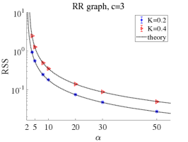
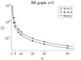
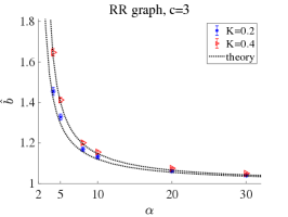
We start by comparing the theoretical and numerical values of \mathcal{E}, Q𝑄Q, and b^^𝑏\hat{b}. In Fig. 6, these quantities are plotted against α𝛼\alpha for K=0.2𝐾0.2K=0.2 and 0.40.40.4 at N=200𝑁200N=200 and c=3𝑐3c=3.

Refer to caption
Refer to caption
Refer to caption
Figure 2: Plots of \mathcal{E} (left), Q𝑄Q (middle), and b^^𝑏\hat{b} (right) against α𝛼\alpha for K=0.2𝐾0.2K=0.2 and 0.40.40.4 at (N,c)=(200,3)𝑁𝑐2003(N,c)=(200,3). Dotted lines and color markers are the theoretical and numerical values, respectively. The agreement between them is fairly good. The left and middle panels are plotted in the double log scale because \mathcal{E} and Q𝑄Q drastically diverge in the limit α2𝛼2\alpha\to 2. The error bars obtained from Nset=100subscript𝑁set100N_{\rm set}=100 datasets are shown, although they tend to be comparable with the size of markers.

In all the plots, the agreement between the theoretical (dotted lines) and numerical (color markers) results is fairly good, supporting the validity of our analytical treatment.

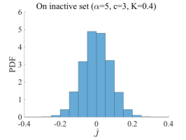
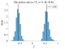
Next, we consider the distributions of the estimators in Fig. 3, which were normalized as probability distribution functions.
Refer to caption
Refer to caption
Refer to caption
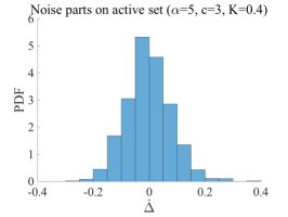
Figure 3: Distribution of the estimators 𝑱^^𝑱\hat{\bm{J}} on the active and inactive sets are given in the left and middle panels, respectively. The right panel is the distribution of the noise part on the active set, {Δ^i=J^iJ¯i}iΩsubscriptsubscript^Δ𝑖subscript^𝐽𝑖subscript¯𝐽𝑖𝑖Ω\{\hat{\Delta}_{i}=\hat{J}_{i}-\bar{J}_{i}\}_{i\in\Omega}. The system parameters are (N,K,α,c)=(200,0.4,5,3)𝑁𝐾𝛼𝑐2000.453(N,K,\alpha,c)=(200,0.4,5,3). The middle and right panels imply that the noise parts obey the zero-mean Gaussian distribution and have no discriminative difference between the active and inactive sets. Here, the histograms are generated from Nset=500subscript𝑁set500N_{\rm set}=500 datasets; from each dataset, the number of obtained estimators is c=3𝑐3c=3 for ΩΩ\Omega while that for Ω¯¯Ω\bar{\Omega} is Nc1=196𝑁𝑐1196N-c-1=196.

The left panel is the distribution of the estimators on the active set ΩΩ\Omega. We can observe that two peaks are located around the theoretical prediction ±b^Kplus-or-minus^𝑏𝐾\pm\hat{b}K. In the middle panel, the estimator distribution on the inactive set Ω¯¯Ω\bar{\Omega} is shown, yielding a Gaussian-like distribution with zero mean. Similar behavior is observed for the noise part on the active set, {Δ^i=J^iJ¯i}iΩsubscriptsubscript^Δ𝑖subscript^𝐽𝑖subscript¯𝐽𝑖𝑖Ω\{\hat{\Delta}_{i}=\hat{J}_{i}-\bar{J}_{i}\}_{i\in\Omega}, the distribution of which is given in the right panel. Here, the mean estimates {J¯i}iΩsubscriptsubscript¯𝐽𝑖𝑖Ω\{\bar{J}_{i}\}_{i\in\Omega} are computed by multiplying the theoretically evaluated bias b^^𝑏\hat{b} by the true coupling {Ji}iΩsubscriptsuperscriptsubscript𝐽𝑖𝑖Ω\{J_{i}^{*}\}_{i\in\Omega}. These observations are again consistent with our theoretical analysis.

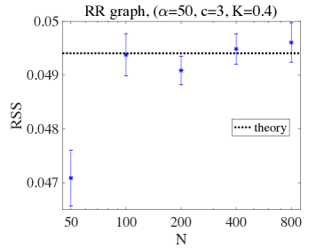
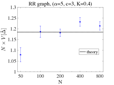
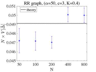
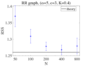
Thirdly, we check the finite size effect. In Fig. 4, against the system size N𝑁N, the RSS and rescaled variance (multiplied by N𝑁N) of the noise parts 𝚫^=𝑱^𝑱¯^𝚫^𝑱¯𝑱\hat{\bm{\Delta}}=\hat{\bm{J}}-\bar{\bm{J}} are plotted in the upper and lower panels, respectively.
Refer to caption
Refer to caption
Refer to caption
Refer to caption
Figure 4: (Upper): Plot of \mathcal{E} against the system size N𝑁N for α=5𝛼5\alpha=5 (left) and 505050 (right) at (K,c)=(0.4,3)𝐾𝑐0.43(K,c)=(0.4,3). The black dotted lines denote the theoretical result and the markers are the numerical ones. The numerical results tend to converge with the theoretical results as the system size grows, although the finite size effect seems to be different between the left and right panels. The error bar is obtained from Nset=500subscript𝑁set500N_{\rm set}=500 datasets for N=50𝑁50N=50200200200, Nset=400subscript𝑁set400N_{\rm set}=400 for N=400𝑁400N=400, and Nset=50subscript𝑁set50N_{\rm set}=50 for N=800𝑁800N=800. (Lower): The rescaled variance (multiplied by N𝑁N) of the noise part 𝚫^=𝑱^𝑱¯^𝚫^𝑱¯𝑱\hat{\bm{\Delta}}=\hat{\bm{J}}-\bar{\bm{J}} is plotted against the system size N𝑁N. The parameters are the same as those of their counterparts in the upper panels. Although in this closeup scale there is a small gap between the numerical and theoretical results within the one standard error, this gap can be eliminated by taking a larger number of samples. Here, the error bar was obtained using the bootstrap method by considering each realization and component of 𝚫^^𝚫\hat{\bm{\Delta}} as i.i.d..

Although the finite size effect behaves in different ways depending on the parameters and quantities, we can see that the numerical results (markers) fairly matched the theoretical values (black dotted lines) as the system size is large. Here, the rescaled variance corresponds to the quantity QTr(C\0)1/N𝑄Trsuperscriptsuperscript𝐶\absent01𝑁Q\mathop{\rm Tr}\left(C^{\backslash 0}\right)^{-1}/N in our theoretical computation, which is consistent with eq. (54). These results again confirm the validity of our computations.

Finally, we have some noteworthy remarks. The results shown in Figs. 3 and 4 imply the possibility of an efficient method of debiasing and hypothesis testing. The bias factor b^^𝑏\hat{b} can be computed from our analytical result, and hence we can debias our estimator in an efficient manner. The residual after debiasing 𝚫^^𝚫\hat{\bm{\Delta}} is considered to obey a Gaussian distribution, as shown in Fig. 3, and is supported by our analytical computations in sec. A. Thus, we can efficiently compute the P-value according to the standard hypothesis testing method, enabling us to judge the relevance of the estimated couplings. Moreover, in the thermodynamic limit N𝑁N\to\infty, we can show that the perfect reconstruction of the teacher’s network is possible for any α>2𝛼2\alpha>2. To do so, we need to evaluate the probability of getting false positives in the estimator. To control false positives, we introduce a constant threshold value Kth(>0)annotatedsubscript𝐾thabsent0K_{\rm th}(>0), and consider estimated couplings with absolute values less than Kthsubscript𝐾thK_{\rm th} as negligible and set to zero; we independently repeat this procedure for all i=1,,N𝑖1𝑁i=1,\cdots,N. Let us evaluate the probability of successfully screening out false positives using this method. The observations so far imply, on the inactive set Ω¯¯Ω\bar{\Omega}, that the estimator behaves as

J^i𝒩(0,σi2N),(iΩ¯),similar-tosubscript^𝐽𝑖𝒩0superscriptsubscript𝜎𝑖2𝑁for-all𝑖¯Ω\displaystyle\hat{J}_{i}\sim\mathcal{N}\left(0,\frac{\sigma_{i}^{2}}{N}\right),~{}(\forall i\in\bar{\Omega}), (72)

where σi2(=O(1))annotatedsuperscriptsubscript𝜎𝑖2absent𝑂1\sigma_{i}^{2}(=O(1)) is the rescaled variance of the estimate, with relation (1/N)iΩ¯σi2QTr(C\0)1/N1𝑁subscript𝑖¯Ωsuperscriptsubscript𝜎𝑖2𝑄Trsuperscriptsuperscript𝐶\absent01𝑁(1/N)\sum_{i\in\bar{\Omega}}\sigma_{i}^{2}\approx Q\mathop{\rm Tr}\left(C^{\backslash 0}\right)^{-1}/N. Hence, the probability of successfully screening out these estimators on Ω¯¯Ω\bar{\Omega} is

iΩ¯Prob(|J^i|<Kth)=iΩ¯(12Nσi2Kth𝑑ze12z22π)subscriptproduct𝑖¯ΩProbsubscript^𝐽𝑖subscript𝐾thsubscriptproduct𝑖¯Ω12superscriptsubscript𝑁superscriptsubscript𝜎𝑖2subscript𝐾thdifferential-d𝑧superscript𝑒12superscript𝑧22𝜋\displaystyle\prod_{i\in\bar{\Omega}}{\rm Prob}\left(|\hat{J}_{i}|<K_{\rm th}\right)=\prod_{i\in\bar{\Omega}}\left(1-2\int_{\sqrt{\frac{N}{\sigma_{i}^{2}}}K_{\rm th}}^{\infty}dz~{}\frac{e^{-\frac{1}{2}z^{2}}}{\sqrt{2\pi}}\right)
iΩ¯(122πe12Nσi2Kth2Nσi2Kth)1,(N).formulae-sequenceabsentsubscriptproduct𝑖¯Ω122𝜋superscript𝑒12𝑁superscriptsubscript𝜎𝑖2superscriptsubscript𝐾th2𝑁superscriptsubscript𝜎𝑖2subscript𝐾th1𝑁\displaystyle\approx\prod_{i\in\bar{\Omega}}\left(1-\frac{2}{\sqrt{2\pi}}\frac{e^{-\frac{1}{2}\frac{N}{\sigma_{i}^{2}}K_{\rm th}^{2}}}{\sqrt{\frac{N}{\sigma_{i}^{2}}}K_{\rm th}}\right)\to 1,~{}(N\to\infty). (73)

The second approximate equality comes from the asymptotic formula of the integral, which can be justified for large N𝑁N. The last limiting behavior holds as long as σisubscript𝜎𝑖\sigma_{i} is bounded from above, because the exponential factor e12Nσi2Kth2superscript𝑒12𝑁superscriptsubscript𝜎𝑖2superscriptsubscript𝐾th2e^{-\frac{1}{2}\frac{N}{\sigma_{i}^{2}}K_{\rm th}^{2}} decays fast enough compared with the number of products |Ω¯|=Nc1¯Ω𝑁𝑐1|\bar{\Omega}|=N-c-1. Hence, we can completely suppress the false positives in the limit N𝑁N\to\infty. Meanwhile, we also desire to accurately reproduce the presence of couplings on ΩΩ\Omega. This can be done by tuning the threshold value Kthsubscript𝐾thK_{\rm th} as smaller than the true coupling strength K𝐾K (the mean estimates 𝑱¯¯𝑱\bar{\bm{J}} are larger than K𝐾K in the absolute value). In practical situations, we do not know the true coupling strength K𝐾K in advance, and thus it is nontrivial to correctly tune Kthsubscript𝐾thK_{\rm th}. In such cases, it may be better to tune Kthsubscript𝐾thK_{\rm th} by monitoring the distribution of estimators such as Fig. 3, and to find a value that effectively separates the modes of distribution. The present theoretical analysis supports this process by manifesting the behavior of estimators in the limit N𝑁N\to\infty.

4.2 ER graph case

For the ER graph with connection probability p=d/N𝑝𝑑𝑁p=d/N, the evaluation of the order parameters and related quantities is slightly more complex than the RR case because of the distributed nature of the connectivity. In the thermodynamic limit, the distribution of connectivity c𝑐c in the ER graph obeys the Poisson distribution:

Ppo(c|d)=eddcc!.subscript𝑃poconditional𝑐𝑑superscript𝑒𝑑superscript𝑑𝑐𝑐\displaystyle P_{\rm po}(c|d)=e^{-d}\frac{d^{c}}{c!}. (74)

The trace of the inverse correlation function fortunately becomes simple in the limit:

1NTrC1Nc=0(c1tanh2Kc+1)Ppo(c|d)=(d1tanh2Kd+1).𝑁1𝑁Trsuperscript𝐶1superscriptsubscript𝑐0𝑐1superscript2𝐾𝑐1subscript𝑃poconditional𝑐𝑑𝑑1superscript2𝐾𝑑1\displaystyle\frac{1}{N}\mathop{\rm Tr}C^{-1}\xrightarrow[]{N\to\infty}\sum_{c=0}^{\infty}\left(\frac{c}{1-\tanh^{2}K}-c+1\right)P_{\rm po}(c|d)=\left(\frac{d}{1-\tanh^{2}K}-d+1\right). (75)

When focusing on spin i𝑖i with connectivity cisubscript𝑐𝑖c_{i} in the ER graph, its associated order parameters are computed by eq. (51) with P(h|ci)𝑃conditionalsuperscriptsubscript𝑐𝑖P(h^{*}|c_{i}) defined in eq. (70), and the RSS is given by

i(ci)=(1b^(ci))2K2+Q(ci)(d1tanh2Kd+1).subscript𝑖subscript𝑐𝑖superscript1^𝑏subscript𝑐𝑖2superscript𝐾2𝑄subscript𝑐𝑖𝑑1superscript2𝐾𝑑1\displaystyle\mathcal{E}_{i}(c_{i})=(1-\hat{b}(c_{i}))^{2}K^{2}+Q(c_{i})\left(\frac{d}{1-\tanh^{2}K}-d+1\right). (76)

This explicit dependence of the order parameter on cisubscript𝑐𝑖c_{i} is the complex point of the ER case. Upon realizing this property, we can easily compute the mean RSS for the whole network, which is written as

mean=1Ni=1NiNc=0{(1b^(c))2K2+(d1tanh2Kd+1)Q(c)}Ppo(c|d).subscriptmean1𝑁superscriptsubscript𝑖1𝑁subscript𝑖𝑁superscriptsubscript𝑐0superscript1^𝑏𝑐2superscript𝐾2𝑑1superscript2𝐾𝑑1𝑄𝑐subscript𝑃poconditional𝑐𝑑\displaystyle\mathcal{E}_{\rm mean}=\frac{1}{N}\sum_{i=1}^{N}\mathcal{E}_{i}\xrightarrow[]{N\to\infty}\sum_{c=0}^{\infty}\left\{(1-\hat{b}(c))^{2}K^{2}+\left(\frac{d}{1-\tanh^{2}K}-d+1\right)Q(c)\right\}P_{\rm po}(c|d). (77)

These provide explicit formulas of the RSSs for the ER case.

As an interesting departure from the RR case, we here examine the connectivity dependence of our quantities of interest. The plots of (c),Q(c)𝑐𝑄𝑐\mathcal{E}(c),Q(c), and b^(c)^𝑏𝑐\hat{b}(c) at (N,α,d,K)=(400,10,4,0.4)𝑁𝛼𝑑𝐾4001040.4(N,\alpha,d,K)=(400,10,4,0.4) are given in Fig. 5.

Refer to caption
Refer to caption
Refer to caption
Figure 5: Plots of \mathcal{E} (left), Q𝑄Q (middle), and b^^𝑏\hat{b} (right) against c𝑐c at (N,α,d)=(400,10,4)𝑁𝛼𝑑400104(N,\alpha,d)=(400,10,4). Black dotted lines and markers are the theoretical and numerical values, respectively; the different colors correspond to different K𝐾K. The agreement between them is fairly good.

In this experiment, we generated ten different ER networks, performed two independent MC samplings, and conducted learning for all i=1,,N𝑖1𝑁i=1,\cdots,N. The error bars were placed using the obtained datasets, and thus Nsetsubscript𝑁setN_{\rm set} varied among different connectivity c𝑐c. The agreement between the theoretical and numerical results is fairly good, supporting our theoretical result. Although a slight deviation at large c𝑐c in (c)𝑐\mathcal{E}(c) and Q(c)𝑄𝑐Q(c) was observed, this was presumably attributed to the finite size effect, which increased at large c𝑐c because of insufficient system size for generating nodes with large c𝑐c. We have tried to control this deviation but found it is difficult to conduct experiments of sufficiently large systems in reasonable time: The generation probability of node with, say, c=13𝑐13c=13 can be estimated as Ppo(13|4)2×10⁴subscript𝑃poconditional1342superscript104P_{\rm po}(13|4)\approx 2\times 10^{-4}, and hence for stably generating networks with such large degree nodes we need at least N5000𝑁5000N\approx 5000, which is too much in our experiment. We thus leave this problem untouched.

We also computed the mean RSS (77) for the whole network. The theoretical value is mean=0.4780subscriptmean0.4780\mathcal{E}_{\rm mean}=0.4780, while the present experimental value is mean=0.4907±0.0041subscriptmeanplus-or-minus0.49070.0041\mathcal{E}_{\rm mean}=0.4907\pm 0.0041. The slight difference between these is again attributed to the finite size effect. Here, the theoretical value was obtained by taking the sum of eq. (77) up to c=20𝑐20c=20; the effect of this truncation was found to be small.

4.3 Square lattice case for comparison

The cavity method in direct problems is known to yield good approximations even for loopy graphs, when correlations among spins are weak; it is sometimes referred to as Bethe approximation. Here, we examined this approximation nature of the present theoretical computation of inverse problems. To this end, we compared our theoretical result for c=4𝑐4c=4 with the simulation result on the square lattice with periodic boundary condition. To avoid possible complexity due to frustration, the present teacher couplings were assumed to be all positive and constant, Ji=K>0,(iΩ)formulae-sequencesuperscriptsubscript𝐽𝑖𝐾0𝑖ΩJ_{i}^{*}=K>0,(i\in\Omega).

In Fig. 6, we plotted \mathcal{E} and b^^𝑏\hat{b} against α𝛼\alpha for K=0.2𝐾0.2K=0.2 on the square lattice of size 20×20202020\times 20, in comparison with our theoretical result (dotted line) computed with the assumption of the tree-like network structure.
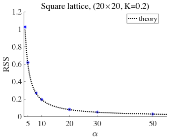
Refer to caption
Refer to caption
Figure 6: Plots of \mathcal{E} (left) and b^^𝑏\hat{b} (right) against α𝛼\alpha for K=0.2𝐾0.2K=0.2 on the square lattice of size 20×20202020\times 20. For comparison, the theoretical results derived by assuming the tree-like structure of the coupling network are plotted as the dotted lines. The agreement between the markers (numerical results) and lines is fairly good. The error bars obtained from Nset=400subscript𝑁set400N_{\rm set}=400 datasets are shown.

The agreement between the theoretical and numerical results is fairly good. This indicates that our theoretical result can be a good approximation even for loopy graphs.

Another interesting phenomenon for loopy graphs is the possible presence of bias in the estimated couplings for spins in Ω¯¯Ω\bar{\Omega}, as discussed in sec. 3.3. To examine this, in the upper panels of Fig. 7 we show the distributions of the coupling estimates corresponding to the next nearest neighbors (NNN) from the center spin s0subscript𝑠0s_{0} in the teacher model for the square lattice (left) and for the RR graph with c=4𝑐4c=4 (right).

Refer to caption
Refer to caption
Refer to caption
Refer to caption
Figure 7: (Upper): Distributions of the NNN estimators for the 20×20202020\times 20 square lattice (left) and for the RR graph with (N,c)=(400,4)𝑁𝑐4004(N,c)=(400,4). In both cases, other parameters are set to be (K,α)=(0.2,5)𝐾𝛼0.25(K,\alpha)=(0.2,5) and Nset=400subscript𝑁set400N_{\rm set}=400. No clear positive/negative tendency is observed in both cases. (Lower). Plots of the mean of the NNN estimate distribution against the system size for the square lattice (left) and RR graph (right). The other parameters are similar to those of the corresponding upper panels. The means are quite small, and no clear deviation from zero is observed. The dataset sizes are Nset=600,600,400,200,40subscript𝑁set60060040020040N_{\rm set}=600,600,400,200,40 for N=100,225,400,900,1600𝑁1002254009001600N=100,225,400,900,1600, respectively. The error bars are obtained using the bootstrap method.

To make a fair comparison, the present teacher couplings for the RR graph case are all positive and constant as the square lattice case. These two distributions are very similar, implying that the bias in coupling estimates for remote spins is, even if it exists in loopy graphs, very weak for the present situation. For further quantitative information, the means of those distributions were plotted against the system size in the lower panels. Again, we observed no clear deviation from zero and no significant difference between the two cases of the square lattice and RR graph. These suggest the practicality of the theoretical results for wider situations than tree-like networks.

4.4 Comparison with interaction screening

We here examine the IS cost function [21, 22], which is another common method for the inverse Ising problem. The IS cost function is given by

IS(x)=ex.superscriptIS𝑥superscript𝑒𝑥\displaystyle\ell^{{\rm IS}}(x)=e^{-x}. (78)

The quantitative comparison with the PL method is of our interest.

In Fig. 8, we plot \mathcal{E}, Q𝑄Q, and b^^𝑏\hat{b} against α𝛼\alpha for the RR graph at (c,K)=(3,0.4)𝑐𝐾30.4(c,K)=(3,0.4), with two theoretical curves of IS (dashed line) and PL (dotted line). Numerical results (asterisks) are also shown to validate the theoretical result of the IS case.
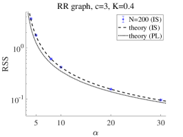
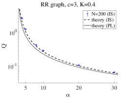
Refer to caption
Refer to caption
Refer to caption
Figure 8: Comparison of the PL and IS results. Plots of \mathcal{E} (left), Q𝑄Q (middle), and b^^𝑏\hat{b} (right) against α𝛼\alpha at (c,K)=(3,0.4)𝑐𝐾30.4(c,K)=(3,0.4) for the RR graph are given. The theoretical curves for PL and IS are described by dotted and dashed lines, respectively. The color markers are the numerical results for the IS case at N=200𝑁200N=200, whose error bars are obtained from Nset=100subscript𝑁set100N_{\rm set}=100 datasets. The consistency of the numerical and theoretical results is fairly good. The IS result provides larger values in all these three quantities than those of PL, implying that IS gives larger error, variance, and bias.

The important observation is that the IS result consistently gives larger values of \mathcal{E}, Q𝑄Q, b^^𝑏\hat{b} than those of PL. This implies that the IS method gives larger error, variance, and bias than PL. Although it is known that IS achieves the optimal scaling of the dataset size M𝑀M [21, 22, 35] necessary for perfect reconstruction of the coupling network structure, it does not necessarily mean the better accuracy in terms of variance/bias. The present analysis demonstrates this in a concise way.

5 Summary and discussion

We proposed a theory to evaluate the reconstruction performance in inverse Ising problems with sparse couplings by maximizing of the pseudolikelihood in the thermodynamic limit. A large part of the theory relies on the statistical mechanical formulation in [24], but we refined the theoretical treatment in the cavity method to handle the teacher model with sparse couplings. The resultant expression requires a full functional form of the cavity field distribution, which is far from Gaussian but was obtained by appropriate consideration of the direct problem counterpart. The theoretical result shows fairly good agreement with numerical experiments conducted on the RR and ER graphs, justifying our theoretical treatment. This agreement holds even for the case of the square lattice, suggesting the practicality of the present result as an approximation for loopy graphs.

The crucial assumptions of our treatment are the asymptotic behavior of the estimator (38) and the paramagnet assumption of the teacher model, leading to the decoupled distributions of the cavity fields. The former assumption implies that the teacher’s couplings can be reconstructed by the student almost perfectly, as discussed at the end of sec. 4.1 according to the hypothesis testing framework, providing a theoretical reasoning to use the inverse Ising framework. The latter assumption requires the smallness of the coupling strength, implying that strongly-correlated datasets cannot be treated by the proposed theory. It will be a challenge to overcome this applicability limitation.

Concerning to the perfect reconstruction of the sparse network in the inverse Ising framework, earlier studies reported similar results in empirical and theoretical ways [29, 35, 36, 37]. Especially, a series of analyses by Wainwright and the collaborators [35, 36, 37] derived the necessary and sufficient conditions for the perfect reconstruction in the high-dimensional limit, clarifying that the necessary size of the dataset scales as M=O(logN)𝑀𝑂𝑁M=O(\log N) when the maximum degree of the network is bounded from above. Compared to this scaling, our result on the scaling M=O(N)𝑀𝑂𝑁M=O(N) is rather conservative. Our formulation, however, has some nontrivial advantages by deriving more detailed information about the system. For example, our formulation can treat the ER graph, the maximum degree of which is not bounded and the proofs established in [35, 36, 37] are not applicable. Our result also clarifies by directly assessing the estimator’s fluctuation that the hypothesis testing can actually achieve the perfect reconstruction, which provides another efficient way of reconstruction than the 1subscript1\ell_{1} regularization used in the above earlier studies. The explicit computation of the bias on the estimator is also another profit. In this way, the present formulation can provide finer information in concrete cases and will be beneficial in wider situations.

For handling real-world datasets, finite magnetizations as well as possible loop structures in the network should be taken into account. For such realistic situations, the computation of (1/N)TrC11𝑁Trsuperscript𝐶1(1/N)\mathop{\rm Tr}C^{-1} and Pcav(h|𝑱)subscript𝑃cavconditionalsuperscriptsuperscript𝑱P_{\rm cav}(h^{*}|\bm{J}^{*}) will be more complicated. For evaluating those quantities, advanced techniques such as Bethe approximation [33, 34], high-temperature expansion, and MC samplings will be useful. The ansatz (38) should be also modified for the case of loopy graphs, as discussed in sec. 3.3. The presented result can be still practical as an approximation for treating such situations, as demonstrated in sec. 4.3. Certain data analysis utilizing these theoretical results will be interesting and useful.

A clear drawback of the estimator treated in this paper is that it is not informative in the region α2𝛼2\alpha\leq 2, as indicated by the divergent RSS in the limit α2+0𝛼20\alpha\to 2+0 shown in sec. 4 and [24]. To overcome this, the use of regularizations will be promising. The 1subscript1\ell_{1} regularization will be particularly useful to control false positives in the estimated couplings. It is also possible to employ hypothesis testing in conjunction with 2subscript2\ell_{2} regularization [38]. An extension of the present analysis to these cases is interesting and will be our focus in future work.

Another interesting extension of the present analysis might be the analysis of the model-mismatched cases where the student model cannot be equal to the teacher one. Even in such cases, some limited information in the teacher, such as the coupling network structure, might be recovered in some conditions [10]. Pursuing this possibility will be interesting because it can provide a better justification for applications of the inverse Ising framework to the analysis of real-world datasets. The analysis of model-mismatched cases may also have a connection to “criticality” observed in earlier studies [39].

The inverse Ising problem or Boltzmann machine has been treated in this paper. Although this model is much simpler than the current models of machine learning communities, we believe that it is important to enhance theoretical knowledge on such simple models to maintain the reliability and interpretability of the results given by machine learning technologies. We hope that our study contributes to this direction, which will lead to a better understanding of and relationship with more complex models.

Acknowledgement

This work was supported by JSPS KAKENHI Nos. 25120013 and 17H00764, and JST CREST Grant Number JPMJCR1912, Japan.

Appendix A Computations for L𝐿L and S𝑆S

For computing L𝐿L, the following decomposition of the cavity fields becomes useful:

h=Qm2qv+m2qz,superscriptsuperscript𝑄superscript𝑚2𝑞subscript𝑣superscript𝑚2𝑞𝑧\displaystyle h^{*}=\sqrt{Q^{*}-\frac{m^{2}}{q}}v_{*}+\sqrt{\frac{m^{2}}{q}}z, (79)
ha=Qqva+qz,superscript𝑎𝑄𝑞subscript𝑣𝑎𝑞𝑧\displaystyle h^{a}=\sqrt{Q-q}v_{a}+\sqrt{q}z, (80)

where va,v,zsubscript𝑣𝑎subscript𝑣𝑧v_{a},v_{*},z are i.i.d Gaussian variables with zero mean and unit variance. It is easy to confirm that this decomposition reproduces the covariances among {h,h1,,hn}superscriptsuperscript1superscript𝑛\{h^{*},h^{1},\cdots,h^{n}\}. Using this and performing the integration with respect to vsubscript𝑣v_{*}, we get

L(Q,Q,q,m)=Dzem2qz12m2q(Dveβ(Qqv+qz))n,𝐿superscript𝑄𝑄𝑞𝑚𝐷𝑧superscript𝑒superscript𝑚2𝑞𝑧12superscript𝑚2𝑞superscript𝐷𝑣superscript𝑒𝛽𝑄𝑞𝑣𝑞𝑧𝑛\displaystyle L(Q^{*},Q,q,m)=\int Dz~{}e^{\sqrt{\frac{m^{2}}{q}}z-\frac{1}{2}\frac{m^{2}}{q}}\left(\int Dv~{}e^{-\beta\ell\left(\sqrt{Q-q}v+\sqrt{q}z\right)}\right)^{n}, (81)

where we use the relation Z0=2e12Qsubscript𝑍02superscript𝑒12superscript𝑄Z_{0}=2e^{\frac{1}{2}Q^{*}}, which was canceled with a factor appearing by the integration of vsubscript𝑣v_{*}. Eq. (26) is easily derived from this.

For computing the entropic term S(C\0,𝑱,Q,q,m)𝑆superscript𝐶\absent0superscript𝑱𝑄𝑞𝑚S(C^{\backslash 0},\bm{J}^{*},Q,q,m), we use the rescaled variable 𝑾=N𝑱𝑾𝑁𝑱\bm{W}=\sqrt{N}\bm{J} and set the integration measure as Tr𝑱=𝑑𝑾subscriptTr𝑱differential-d𝑾\mathop{\rm Tr}_{\bm{J}}=\int d\bm{W}. Here, we use the uniform measure because in the present setting the student has no prior information about the teacher couplings. If certain prior knowledge is available such as the teacher coupling sparseness, it can be suitable to introduce another measure such as Laplace prior. Further, we represent the delta functions by the Fourier expressions as follows:

δ(Q1Ni,jCij\0WiaWja)=C1𝑑Q~e12NQ~Q12Q~i,iCij\0WiaWja,𝛿𝑄1𝑁subscript𝑖𝑗subscriptsuperscript𝐶\absent0𝑖𝑗subscriptsuperscript𝑊𝑎𝑖superscriptsubscript𝑊𝑗𝑎subscript𝐶1differential-d~𝑄superscript𝑒12𝑁~𝑄𝑄12~𝑄subscript𝑖𝑖subscriptsuperscript𝐶\absent0𝑖𝑗subscriptsuperscript𝑊𝑎𝑖superscriptsubscript𝑊𝑗𝑎\displaystyle\delta\left(Q-\frac{1}{N}\sum_{i,j}C^{\backslash 0}_{ij}W^{a}_{i}W_{j}^{a}\right)=C_{1}\int d\tilde{Q}~{}e^{\frac{1}{2}N\tilde{Q}Q-\frac{1}{2}\tilde{Q}\sum_{i,i}C^{\backslash 0}_{ij}W^{a}_{i}W_{j}^{a}}, (82a)
δ(q1Ni,jCij\0WiaWjb)=C2𝑑q~eNq~q+q~i,jCij\0WiaWjb,𝛿𝑞1𝑁subscript𝑖𝑗subscriptsuperscript𝐶\absent0𝑖𝑗subscriptsuperscript𝑊𝑎𝑖superscriptsubscript𝑊𝑗𝑏subscript𝐶2differential-d~𝑞superscript𝑒𝑁~𝑞𝑞~𝑞subscript𝑖𝑗subscriptsuperscript𝐶\absent0𝑖𝑗subscriptsuperscript𝑊𝑎𝑖superscriptsubscript𝑊𝑗𝑏\displaystyle\delta\left(q-\frac{1}{N}\sum_{i,j}C^{\backslash 0}_{ij}W^{a}_{i}W_{j}^{b}\right)=C_{2}\int d\tilde{q}~{}e^{-N\tilde{q}q+\tilde{q}\sum_{i,j}C^{\backslash 0}_{ij}W^{a}_{i}W_{j}^{b}}, (82b)
δ(m1Ni,jCij\0WiWja)=C2𝑑m~eNm~m+m~i,jCij\0WiWja,𝛿𝑚1𝑁subscript𝑖𝑗subscriptsuperscript𝐶\absent0𝑖𝑗subscriptsuperscript𝑊𝑖superscriptsubscript𝑊𝑗𝑎subscript𝐶2differential-d~𝑚superscript𝑒𝑁~𝑚𝑚~𝑚subscript𝑖𝑗subscriptsuperscript𝐶\absent0𝑖𝑗subscriptsuperscript𝑊𝑖superscriptsubscript𝑊𝑗𝑎\displaystyle\delta\left(m-\frac{1}{N}\sum_{i,j}C^{\backslash 0}_{ij}W^{*}_{i}W_{j}^{a}\right)=C_{2}\int d\tilde{m}~{}e^{-N\tilde{m}m+\tilde{m}\sum_{i,j}C^{\backslash 0}_{ij}W^{*}_{i}W_{j}^{a}}, (82c)

where the integration contour is the imaginary axis and C1,C2subscript𝐶1subscript𝐶2C_{1},C_{2} are appropriate normalization constants; however, these points are irrelevant and ignored hereafter. Inserting this into eq. (23), we get

eNS=𝑑Q~𝑑q~𝑑m~eSXad𝑾aeU,superscript𝑒𝑁𝑆differential-d~𝑄differential-d~𝑞differential-d~𝑚superscript𝑒subscript𝑆𝑋subscriptproduct𝑎𝑑superscript𝑾𝑎superscript𝑒𝑈\displaystyle e^{NS}=\int d\tilde{Q}d\tilde{q}d\tilde{m}~{}e^{S_{X}}\int\prod_{a}d\bm{W}^{a}~{}e^{U}, (83)

where

𝒮X=N(12nQ^Q12n(n1)q~qnm~m),subscript𝒮𝑋𝑁12𝑛^𝑄𝑄12𝑛𝑛1~𝑞𝑞𝑛~𝑚𝑚\displaystyle\mathcal{S}_{X}=N\left(\frac{1}{2}n\hat{Q}Q-\frac{1}{2}n(n-1)\tilde{q}q-n\tilde{m}m\right), (84)
U=12Q~a(𝑾a)C\0𝑾a+q~a<b(𝑾a)C\0𝑾b+m~a(𝑱)C\0𝑾a𝑈12~𝑄subscript𝑎superscriptsuperscript𝑾𝑎topsuperscript𝐶\absent0superscript𝑾𝑎~𝑞subscript𝑎𝑏superscriptsuperscript𝑾𝑎topsuperscript𝐶\absent0superscript𝑾𝑏~𝑚subscript𝑎superscriptsuperscript𝑱topsuperscript𝐶\absent0superscript𝑾𝑎\displaystyle U=-\frac{1}{2}\tilde{Q}\sum_{a}\left(\bm{W}^{a}\right)^{\top}C^{\backslash 0}\bm{W}^{a}+\tilde{q}\sum_{a<b}\left(\bm{W}^{a}\right)^{\top}C^{\backslash 0}\bm{W}^{b}+\tilde{m}\sum_{a}\left(\bm{J}^{*}\right)^{\top}C^{\backslash 0}\bm{W}^{a}
=12(Q~+q~)a(𝑾a)C\0𝑾a+12q~a,b(𝑾a)C\0𝑾b+m~a(𝑱)C\0𝑾a.absent12~𝑄~𝑞subscript𝑎superscriptsuperscript𝑾𝑎topsuperscript𝐶\absent0superscript𝑾𝑎12~𝑞subscript𝑎𝑏superscriptsuperscript𝑾𝑎topsuperscript𝐶\absent0superscript𝑾𝑏~𝑚subscript𝑎superscriptsuperscript𝑱topsuperscript𝐶\absent0superscript𝑾𝑎\displaystyle=-\frac{1}{2}(\tilde{Q}+\tilde{q})\sum_{a}\left(\bm{W}^{a}\right)^{\top}C^{\backslash 0}\bm{W}^{a}+\frac{1}{2}\tilde{q}\sum_{a,b}\left(\bm{W}^{a}\right)^{\top}C^{\backslash 0}\bm{W}^{b}+\tilde{m}\sum_{a}\left(\bm{J}^{*}\right)^{\top}C^{\backslash 0}\bm{W}^{a}. (85)

To decouple different replicas and components of {𝑾a}asubscriptsuperscript𝑾𝑎𝑎\{\bm{W}^{a}\}_{a}, we use the expression C\0=OΛOsuperscript𝐶\absent0superscript𝑂topΛ𝑂C^{\backslash 0}=O^{\top}\Lambda O, where ΛΛ\Lambda is the diagonal matrix consisting of the eigenvalues {λi}isubscriptsubscript𝜆𝑖𝑖\{\lambda_{i}\}_{i} and O𝑂O is the appropriate orthogonal matrix. Performing the variable transformation 𝑾~=O𝑾~𝑾𝑂𝑾\tilde{\bm{W}}=O\bm{W} and applying the Hubbard–Stratonovich transformation, we get

ad𝑾aeU=iDziad𝑾~ae12(Q~+q~)aiλi(W~ia)2+ai(λiW~im~+λiq~zi)W~iasubscriptproduct𝑎𝑑superscript𝑾𝑎superscript𝑒𝑈subscriptproduct𝑖𝐷subscript𝑧𝑖subscriptproduct𝑎𝑑superscript~𝑾𝑎superscript𝑒12~𝑄~𝑞subscript𝑎subscript𝑖subscript𝜆𝑖superscriptsubscriptsuperscript~𝑊𝑎𝑖2subscript𝑎subscript𝑖subscript𝜆𝑖subscriptsuperscript~𝑊𝑖~𝑚subscript𝜆𝑖~𝑞subscript𝑧𝑖subscriptsuperscript~𝑊𝑎𝑖\displaystyle\int\prod_{a}d\bm{W}^{a}~{}e^{U}=\int\prod_{i}Dz_{i}\int\prod_{a}d\tilde{\bm{W}}^{a}~{}e^{-\frac{1}{2}(\tilde{Q}+\tilde{q})\sum_{a}\sum_{i}\lambda_{i}\left(\tilde{W}^{a}_{i}\right)^{2}+\sum_{a}\sum_{i}\left(\lambda_{i}\tilde{W}^{*}_{i}\tilde{m}+\sqrt{\lambda_{i}\tilde{q}}z_{i}\right)\tilde{W}^{a}_{i}}
=iDzieni{12(λiW~im~+q~zi)2(Q~+q~)+12(log2πlogλilog(Q~+q~))}absentsubscriptproduct𝑖𝐷subscript𝑧𝑖superscript𝑒𝑛subscript𝑖12superscriptsubscript𝜆𝑖subscriptsuperscript~𝑊𝑖~𝑚~𝑞subscript𝑧𝑖2~𝑄~𝑞122𝜋subscript𝜆𝑖~𝑄~𝑞\displaystyle=\int\prod_{i}Dz_{i}~{}e^{n\sum_{i}\left\{\frac{1}{2}\frac{\left(\sqrt{\lambda_{i}}\tilde{W}^{*}_{i}\tilde{m}+\sqrt{\tilde{q}}z_{i}\right)^{2}}{\left(\tilde{Q}+\tilde{q}\right)}+\frac{1}{2}\left(\log 2\pi-\log\lambda_{i}-\log(\tilde{Q}+\tilde{q})\right)\right\}}
=eN2log(1nq~Q~+q~)+12niλi(W~i)2m~2Q~+q~(1n)+n2i(log2πlogλilog(Q~+q~))e𝒮J.absentsuperscript𝑒𝑁21𝑛~𝑞~𝑄~𝑞12𝑛subscript𝑖subscript𝜆𝑖superscriptsubscriptsuperscript~𝑊𝑖2superscript~𝑚2~𝑄~𝑞1𝑛𝑛2subscript𝑖2𝜋subscript𝜆𝑖~𝑄~𝑞superscript𝑒subscript𝒮𝐽\displaystyle=e^{-\frac{N}{2}\log\left(1-\frac{n\tilde{q}}{\tilde{Q}+\tilde{q}}\right)+\frac{1}{2}n\sum_{i}\frac{\lambda_{i}\left(\tilde{W}^{*}_{i}\right)^{2}\tilde{m}^{2}}{\tilde{Q}+\tilde{q}(1-n)}+\frac{n}{2}\sum_{i}\left(\log 2\pi-\log\lambda_{i}-\log(\tilde{Q}+\tilde{q})\right)}\equiv e^{\mathcal{S}_{J}}. (86)

Note that this quadratic form with respect to 𝑾~~𝑾\tilde{\bm{W}} implies that 𝑾~~𝑾\tilde{\bm{W}} essentially obeys Gaussian, and thus the estimator 𝑱^^𝑱\hat{\bm{J}} also does. This knowledge of the distribution can be used for hypothesis testing as addressed in the main text.

In the thermodynamic limit N𝑁N\to\infty, we can use the saddle-point (or Laplace) method to avoid the explicit integrations with respect to Q~,q~,m~~𝑄~𝑞~𝑚\tilde{Q},\tilde{q},\tilde{m}. This yields

S=ExtrQ~,q~,m~{𝒮X+𝒮JN}=ExtrQ~,q~,m~{12nQ~Q12n(n1)q~qnm~m12log(1nq~Q~+q~)\displaystyle S=\mathop{\rm Extr}_{\tilde{Q},\tilde{q},\tilde{m}}\left\{\frac{\mathcal{S}_{X}+\mathcal{S}_{J}}{N}\right\}=\mathop{\rm Extr}_{\tilde{Q},\tilde{q},\tilde{m}}\Bigg{\{}\frac{1}{2}n\tilde{Q}Q-\frac{1}{2}n(n-1)\tilde{q}q-n\tilde{m}m-\frac{1}{2}\log\left(1-\frac{n\tilde{q}}{\tilde{Q}+\tilde{q}}\right)
+12nQm~2Q~+q~(1n)+n2(log2πlog(Q~+q~))n2NTrlogC\0}.\displaystyle+\frac{1}{2}n\frac{Q^{*}\tilde{m}^{2}}{\tilde{Q}+\tilde{q}(1-n)}+\frac{n}{2}\left(\log 2\pi-\log(\tilde{Q}+\tilde{q})\right)-\frac{n}{2N}\mathop{\rm Tr}\log C^{\backslash 0}\Bigg{\}}. (87)

where we used the relations iλi(W~i)2=NQ,ilogλi=TrlogC\0formulae-sequencesubscript𝑖subscript𝜆𝑖superscriptsubscriptsuperscript~𝑊𝑖2𝑁superscript𝑄subscript𝑖subscript𝜆𝑖Trsuperscript𝐶\absent0\sum_{i}\lambda_{i}\left(\tilde{W}^{*}_{i}\right)^{2}=NQ^{*},~{}\sum_{i}\log\lambda_{i}=\mathop{\rm Tr}\log C^{\backslash 0}. The limit n0𝑛0n\to 0 leads to

limn0Sn=ExtrQ~,q~,m~{12Q~Q+12q~qm~m+12q~+Qm~2Q~+q~\displaystyle\lim_{n\to 0}\frac{S}{n}=\mathop{\rm Extr}_{\tilde{Q},\tilde{q},\tilde{m}}\Bigg{\{}\frac{1}{2}\tilde{Q}Q+\frac{1}{2}\tilde{q}q-\tilde{m}m+\frac{1}{2}\frac{\tilde{q}+Q^{*}\tilde{m}^{2}}{\tilde{Q}+\tilde{q}}
+12(log2πlog(Q~+q~))12NTrlogC\0},\displaystyle+\frac{1}{2}\left(\log 2\pi-\log(\tilde{Q}+\tilde{q})\right)-\frac{1}{2N}\mathop{\rm Tr}\log C^{\backslash 0}\Bigg{\}}, (88)

and the extremization condition gives

Q~=Q2q+m2/Q(Qq)2,q~=qm2/Q(Qq)2,m~=m/QQq.formulae-sequence~𝑄𝑄2𝑞superscript𝑚2superscript𝑄superscript𝑄𝑞2formulae-sequence~𝑞𝑞superscript𝑚2superscript𝑄superscript𝑄𝑞2~𝑚𝑚superscript𝑄𝑄𝑞\displaystyle\tilde{Q}=\frac{Q-2q+m^{2}/Q^{*}}{(Q-q)^{2}},~{}\tilde{q}=\frac{q-m^{2}/Q^{*}}{(Q-q)^{2}},~{}\tilde{m}=\frac{m/Q^{*}}{Q-q}. (89)

Substituting these relations into eq. (88), we obtain eq. (25). If we ignore the terms related to m𝑚m and m~~𝑚\tilde{m}, we have eq. (48).

Appendix B Derivation of macroscopic parameters R𝑅R and ρ𝜌\rho

To derive the expressions of R𝑅R and ρ𝜌\rho, we can employ the technique of auxiliary variables. We introduce two terms hRa(𝑾a)𝑾asubscript𝑅subscript𝑎superscriptsuperscript𝑾𝑎topsuperscript𝑾𝑎h_{R}\sum_{a}\left(\bm{W}^{a}\right)^{\top}\bm{W}^{a} and hρa(𝑾)𝑾asubscript𝜌subscript𝑎superscriptsuperscript𝑾topsuperscript𝑾𝑎h_{\rho}\sum_{a}\left(\bm{W}^{*}\right)^{\top}\bm{W}^{a} in eq. (85), and perform the same line of computations as in sec. A. As a result, the entropic term is modified to the following expression:

limn0Sn=ExtrQ~,q~,m~{12Q~Q+12q~qm~m\displaystyle\lim_{n\to 0}\frac{S}{n}=\mathop{\rm Extr}_{\tilde{Q},\tilde{q},\tilde{m}}\Bigg{\{}\frac{1}{2}\tilde{Q}Q+\frac{1}{2}\tilde{q}q-\tilde{m}m
+12Ni((m~λi+hρ)2(W~i)2+λiq~(Q~+q~)λi2hR+log2πlog((Q~+q~)(λi2hR)))}.\displaystyle+\frac{1}{2N}\sum_{i}\left(\frac{(\tilde{m}\lambda_{i}+h_{\rho})^{2}\left(\tilde{W}^{*}_{i}\right)^{2}+\lambda_{i}\tilde{q}}{(\tilde{Q}+\tilde{q})\lambda_{i}-2h_{R}}+\log 2\pi-\log\left((\tilde{Q}+\tilde{q})(\lambda_{i}-2h_{R})\right)\right)\Bigg{\}}. (90)

Taking the differentiation with respect to hρsubscript𝜌h_{\rho} and taking the limit hρ,hR0subscript𝜌subscript𝑅0h_{\rho},h_{R}\to 0, we get

ρ=limhρ,hR0hρlimn0Sn=1Nim~(W~i)2Q~+q~=mQR.𝜌subscriptsubscript𝜌subscript𝑅0subscript𝜌subscript𝑛0𝑆𝑛1𝑁subscript𝑖~𝑚superscriptsubscriptsuperscript~𝑊𝑖2~𝑄~𝑞𝑚superscript𝑄superscript𝑅\displaystyle\rho=\lim_{h_{\rho},h_{R}\to 0}\frac{\partial}{\partial h_{\rho}}\lim_{n\to 0}\frac{S}{n}=\frac{1}{N}\sum_{i}\frac{\tilde{m}\left(\tilde{W}^{*}_{i}\right)^{2}}{\tilde{Q}+\tilde{q}}=\frac{m}{Q^{*}}R^{*}. (91)

The last expression is obtained by using eq. (89). Similarly,

R=limhρ,hR0hRlimn0Sn=1Ni(m~2(W~i)2(Q~+q~)2+Q~+2q~(Q~+q~)21λi)𝑅subscriptsubscript𝜌subscript𝑅0subscript𝑅subscript𝑛0𝑆𝑛1𝑁subscript𝑖superscript~𝑚2superscriptsubscriptsuperscript~𝑊𝑖2superscript~𝑄~𝑞2~𝑄2~𝑞superscript~𝑄~𝑞21subscript𝜆𝑖\displaystyle R=\lim_{h_{\rho},h_{R}\to 0}\frac{\partial}{\partial h_{R}}\lim_{n\to 0}\frac{S}{n}=\frac{1}{N}\sum_{i}\left(\frac{\tilde{m}^{2}\left(\tilde{W}^{*}_{i}\right)^{2}}{\left(\tilde{Q}+\tilde{q}\right)^{2}}+\frac{\tilde{Q}+2\tilde{q}}{\left(\tilde{Q}+\tilde{q}\right)^{2}}\frac{1}{\lambda_{i}}\right)
=(mQ)2R+(Qm2Q)1NTr(C\0)1.absentsuperscript𝑚superscript𝑄2superscript𝑅𝑄superscript𝑚2superscript𝑄1𝑁Trsuperscriptsuperscript𝐶\absent01\displaystyle=\left(\frac{m}{Q^{*}}\right)^{2}R^{*}+\left(Q-\frac{m^{2}}{Q^{*}}\right)\frac{1}{N}\mathop{\rm Tr}\left(C^{\backslash 0}\right)^{-1}. (92)

These give eq. (32).

In the sparse case, we need to compute iΩ¯Δi2subscript𝑖¯ΩsuperscriptsubscriptΔ𝑖2\sum_{i\in\bar{\Omega}}\Delta_{i}^{2} for computing the RSS. By construction, this is equivalent with R𝑅R when m𝑚m is absent. Hence iΩ¯Δi2subscript𝑖¯ΩsuperscriptsubscriptΔ𝑖2\sum_{i\in\bar{\Omega}}\Delta_{i}^{2} is given by putting m=0𝑚0m=0 in eq. (92), leading to eq. (54).

Appendix C Details of numerical experiments

The actual experimental procedures are summarized as follows. We first generated a random graph and the teacher couplings on it, and obtained spin snapshots using MC sampling. Then, we randomly chose a center spin s0subscript𝑠0s_{0} from the whole spins and learned the couplings connected to s0subscript𝑠0s_{0} by minimizing the PL cost function defined with a dataset obtained from the sampled spin configurations. This single sequence of operations provided single values of the quantities of interest, such as \mathcal{E} and Q𝑄Q. To obtain the error bars of those quantities, we repeated this sequence many times. Here, the experiment had three different sources of fluctuations: the generated teacher model (graph shape and couplings), the choice of the center spin, and the MC sampling. We did not discriminate between these three fluctuations unless explicitly mentioned, and we defined the error bar as the standard error among the obtained values according to their recurrence; the number of datasets obtained this way is hereafter denoted as Nsetsubscript𝑁setN_{\rm set}. In the MC sampling, we started from a random initial configuration and updated the state by the standard Metropolis method; one MC step (MCS) is defined by N𝑁N trial flips of spins, where N𝑁N is the total number of spins. We discarded the first 105superscript10510^{5} MCSs as burn-in to avoid systematic errors from the initialization. Furthermore, to avoid possible correlations in samples, each dataset for learning was generated by subsampling from a much larger dataset, which consists of all the configurations recorded after every few numbers of MCS. The size of the subsampled dataset was chosen to be at least five times smaller than that of the larger dataset. The optimization algorithm is a standard trust-region method using the second-order expansion of the objective function.

References

  • [1] Elad Schneidman, Michael J Berry, Ronen Segev, and William Bialek. Weak pairwise correlations imply strongly correlated network states in a neural population. Nature, 440(7087):1007–1012, apr 2006.
  • [2] Jonathon Shlens, Greg D Field, Jeffrey L Gauthier, Matthew I Grivich, Dumitru Petrusca, Alexander Sher, Alan M Litke, and E J Chichilnisky. The structure of multi-neuron firing patterns in primate retina. J. Neurosci., 26(32):8254–8266, aug 2006.
  • [3] Aonan Tang, David Jackson, Jon Hobbs, Wei Chen, Jodi L Smith, Hema Patel, Anita Prieto, Dumitru Petrusca, Matthew I Grivich, Alexander Sher, Pawel Hottowy, Wladyslaw Dabrowski, Alan M Litke, and John M Beggs. A maximum entropy model applied to spatial and temporal correlations from cortical networks in vitro. J. Neurosci., 28(2):505–518, jan 2008.
  • [4] Liberty S Hamilton, Jascha Sohl-Dickstein, Alexander G Huth, Vanessa M Carels, Karl Deisseroth, and Shaowen Bao. Optogenetic activation of an inhibitory network enhances feedforward functional connectivity in auditory cortex. Neuron, 80(4):1066–1076, 2013.
  • [5] Takamitsu Watanabe, Satoshi Hirose, Hiroyuki Wada, Yoshio Imai, Toru Machida, Ichiro Shirouzu, Seiki Konishi, Yasushi Miyashita, and Naoki Masuda. A pairwise maximum entropy model accurately describes resting-state human brain networks. Nat. Commun., 4(May 2012):1370, jan 2013.
  • [6] Takamitsu Watanabe, Naoki Masuda, Fukuda Megumi, Ryota Kanai, and Geraint Rees. Energy landscape and dynamics of brain activity during human bistable perception. Nat. Commun., 5, jan 2014.
  • [7] Gašper Tkačik, Olivier Marre, Dario Amodei, Elad Schneidman, William Bialek, and Michael J. Berry. Searching for collective behavior in a large network of sensory neurons. PLoS Comput. Biol., 10(1):e1003408, jan 2014.
  • [8] Gaia Tavoni, Ulisse Ferrari, Francesco P. Battaglia, Simona Cocco, and Rémi Monasson. Inferred model of the prefrontal cortex activity unveils cell assemblies and memory replay. bioRxiv, 2015.
  • [9] Yu Terada, Tomoyuki Obuchi, Takuya Isomura, and Yoshiyuki Kabashima. Objective procedure for reconstructing couplings in complex systems. arXiv preprint arXiv:1803.04738, 2018.
  • [10] Yu Terada, Tomoyuki Obuchi, Takuya Isomura, and Yoshiyuki Kabashima. Objective and efficient inference for couplings in neuronal networks. In S. Bengio, H. Wallach, H. Larochelle, K. Grauman, N. Cesa-Bianchi, and R. Garnett, editors, Advances in Neural Information Processing Systems 31, pages 4971–4980. Curran Associates, Inc., 2018.
  • [11] Julian Besag. Spatial interaction and the statistical analysis of lattice systems. Journal of the Royal Statistical Society: Series B (Methodological), 36(2):192–225, 1974.
  • [12] Hilbert J. Kappen and Francisco de Borja Rodríguez. Efficient learning in Boltzmann machines using linear response theory. Neural Computation, 10(5):1137–1156, 1998.
  • [13] Toshiyuki Tanaka. Mean-field theory of Boltzmann machine learning. Physical Review E, 58(2):2302, 1998.
  • [14] Geoffrey E. Hinton. Training products of experts by minimizing contrastive divergence. Neural Computation, 14(8):1771–1800, 2002.
  • [15] Tamara Broderick, Miroslav Dudik, Gasper Tkacik, Robert E Schapire, and William Bialek. Faster solutions of the inverse pairwise Ising problem. arXiv preprint arXiv:0712.2437, 2007.
  • [16] Vitor Sessak and Rémi Monasson. Small-correlation expansions for the inverse Ising problem. Journal of Physics A: Mathematical and Theoretical, 42(5):055001, 2009.
  • [17] Yasser Roudi and John Hertz. Mean field theory for nonequilibrium network reconstruction. Phys. Rev. Lett., 106:048702, Jan 2011.
  • [18] M Mézard and J Sakellariou. Exact mean-field inference in asymmetric kinetic Ising systems. Journal of Statistical Mechanics: Theory and Experiment, 2011(07):L07001, jul 2011.
  • [19] S. Cocco and R. Monasson. Adaptive cluster expansion for inferring Boltzmann machines with noisy data. Phys. Rev. Lett., 106:090601, Mar 2011.
  • [20] Erik Aurell and Magnus Ekeberg. Inverse Ising inference using all the data. Phys. Rev. Lett., 108:090201, Mar 2012.
  • [21] Marc Vuffray, Sidhant Misra, Andrey Lokhov, and Michael Chertkov. Interaction screening: Efficient and sample-optimal learning of Ising models. In Advances in Neural Information Processing Systems, pages 2595–2603, 2016.
  • [22] Andrey Y Lokhov, Marc Vuffray, Sidhant Misra, and Michael Chertkov. Optimal structure and parameter learning of Ising models. Science advances, 4(3):e1700791, 2018.
  • [23] Marc Vuffray, Sidhant Misra, and Andrey Y. Lokhov. Efficient learning of discrete graphical models. CoRR, abs/1902.00600, 2019.
  • [24] Ludovica Bachschmid-Romano and Manfred Opper. A statistical physics approach to learning curves for the inverse Ising problem. Journal of Statistical Mechanics: Theory and Experiment, 2017(6):063406, 2017.
  • [25] Ludovica Bachschmid-Romano and Manfred Opper. Learning of couplings for random asymmetric kinetic Ising models revisited: random correlation matrices and learning curves. Journal of Statistical Mechanics: Theory and Experiment, 2015(9):P09016, 2015.
  • [26] Johannes Berg. Statistical mechanics of the inverse Ising problem and the optimal objective function. Journal of Statistical Mechanics: Theory and Experiment, 2017(8):083402, aug 2017.
  • [27] Thomas M Cover and Joy A Thomas. Elements of Information Theory. John Wiley & Sons, 2012.
  • [28] H Chau Nguyen, Riccardo Zecchina, and Johannes Berg. Inverse statistical problems: from the inverse Ising problem to data science. Advances in Physics, 66(3):197–261, 2017.
  • [29] Aurélien Decelle and Federico Ricci-Tersenghi. Pseudolikelihood decimation algorithm improving the inference of the interaction network in a general class of Ising models. Physical review letters, 112(7):070603, 2014.
  • [30] Aapo Hyvärinen. Consistency of pseudolikelihood estimation of fully visible Boltzmann machines. Neural Computation, 18(10):2283–2292, 2006.
  • [31] Manfred Opper and David Saad. Advanced Mean Field Methods : Theory and Practice. Neural information processing series. MIT Press, 2001.
  • [32] Marc Mezard and Andrea Montanari. Information, Physics, and Computation. Oxford University Press, 2009.
  • [33] Federico Ricci-Tersenghi. The Bethe approximation for solving the inverse Ising problem: a comparison with other inference methods. Journal of Statistical Mechanics: Theory and Experiment, 2012(08):P08015, 2012.
  • [34] H Chau Nguyen and Johannes Berg. Bethe–Peierls approximation and the inverse ising problem. Journal of Statistical Mechanics: Theory and Experiment, 2012(03):P03004, 2012.
  • [35] Narayana P Santhanam and Martin J Wainwright. Information-theoretic limits of selecting binary graphical models in high dimensions. IEEE Transactions on Information Theory, 58(7):4117–4134, 2012.
  • [36] Martin J Wainwright, Michael I Jordan, et al. Graphical models, exponential families, and variational inference. Foundations and Trends® in Machine Learning, 1(1–2):1–305, 2008.
  • [37] Pradeep Ravikumar, Martin J Wainwright, and John D Lafferty. High-dimensional Ising model selection using 1subscript1\ell_{1}-regularized logistic regression. The Annals of Statistics, 38(3):1287–1319, 2010.
  • [38] Yingying Xu, Santeri Puranen, Jukka Corander, and Yoshiyuki Kabashima. Inverse finite-size scaling for high-dimensional significance analysis. Physical Review E, 97(6):062112, 2018.
  • [39] Iacopo Mastromatteo and Matteo Marsili. On the criticality of inferred models. Journal of Statistical Mechanics: Theory and Experiment, 2011(10):P10012, 2011.