Neural Subgraph Isomorphism Counting

Abstract.

In this paper, we study a new graph learning problem: learning to count subgraph isomorphisms. Different from other traditional graph learning problems such as node classification and link prediction, subgraph isomorphism counting is NP-complete and requires more global inference to oversee the whole graph. To make it scalable for large-scale graphs and patterns, we propose a learning framework that augments different representation learning architectures and iteratively attends pattern and target data graphs to memorize intermediate states of subgraph isomorphism searching for global counting. We develop both small graphs ($\leq$ 1,024 subgraph isomorphisms in each) and large graphs ($\leq$ 4,096 subgraph isomorphisms in each) sets to evaluate different representation and interaction modules. A mutagenic compound dataset, MUTAG, is also used to evaluate neural models and demonstrate the success of transfer learning. While the learning based approach is inexact, we are able to generalize to count large patterns and data graphs in linear time compared to the exponential time of the original NP-complete problem. Experimental results show that learning based subgraph isomorphism counting can speed up the traditional algorithm, VF2, 10-1,000 times with acceptable errors. Domain adaptation based on fine-tuning also shows the usefulness of our approach in real-world applications.

1. Introduction

Counting subgraph isomorphisms aims at determining the number of subgraphs of a given graph that match (i.e., be isomorphic to) a specific pattern graph of interest. It is one of the useful graph-related tasks for knowledge discovery and data mining applications, e.g., discovering protein interactions in bioinformatics (Milo et al., 2002; Alon et al., 2008), finding active chemical compounds for new drug development in chemoinformatics (Huan et al., 2003), and mining social structures in online social network analysis (Kuramochi and Karypis, 2004). Moreover, finding sub-structures are useful for heterogeneous information networks (HINs) such as knowledge graphs and recommender systems (Fang et al., 2016; Huang et al., 2016; Jiang et al., 2017; Zhao et al., 2017). The rich types on HIN’s schema provide meaningful semantics so that counting itself is valuable for a variety types of queries. For example, in a knowledge graph, we can answer questions like “how many languages are there in Africa spoken by people living near banks of the Nile River?” On a social network, a query like “number of pairs of friends, among them one likes a comic, and the other one likes its movie adaptation” may help briefing an advertisement targeting.

However, previous studies on similar tasks are often under specific constraints, and discussions for general patterns on large heterogeneous graphs are limited. Particularly, former studies on counting reduce to small subgraphs with 3-5 nodes as motifs (without considering isomorphisms) (Milo et al., 2002) or graphlets (limited to induced subgraphs) (Przulj et al., 2006). Moreover, although customized pattern mining algorithms or graph database indexing based approaches may tackle the general problem of subgraph isomorphism (Ullmann, 1976; Cordella et al., 2004; He and Singh, 2008; Han et al., 2013; Carletti et al., 2018), all such algorithms struggle with scaling up to larger graphs due to the NP-complete nature of the task. To extend to larger graphs under the more general and theoretically fundamental setting, alternative scalable methods are required. Specifically, we turn to approximate the answer by machine learning.

Learning with graphs has recently drawn much attention as neural approaches to representation learning have been proven to be effective for complex data structures (Niepert et al., 2016; Kipf and Welling, 2017; Hamilton et al., 2017b; Schlichtkrull et al., 2018; Velickovic et al., 2018; Xu et al., 2019). Admittedly, most of existing graph representation learning algorithms focus on tasks like node classification and link prediction (Hamilton et al., 2017a) that information from local structure is enough for making inference. Such tasks are different from ours which is to count over the whole graph. However, recently it has been demonstrated that, more challenging reasoning problems that involve global inference, such as summary statistics, relational argmax, dynamic programming, and the NP-hard subset sum, can be elegantly solved by learning with properly designed architectures (Xu et al., 2020). The results are inspiring and encouraging. However, there are still challenges lying ahead to the target to count subgraph isomorphisms with machine learning:

$\bullet$ Typical sizes of existing datasets are limited, and far from enough to train a graph neural network. Meanwhile, it is non-trivial to generate sufficient training data for this problem due to the difficulty to obtain the ground truth, compared with other graph learning problems such as shortest path (Graves et al., 2016) or centrality (Fan et al., 2019).

$\bullet$ Appropriate inductive bias must be carefully selected for such challenging task (Battaglia et al., 2018). Therefore, following considerations should be taken into account: First, as the general case of heterogeneous node types and edge types being considered, to represent and discriminate nodes and edges with neighborhood structure, stronger and more complicated representation learning techniques should be applied. Second, the task is not performed on a single graph but involves with an extra pattern. Therefore, the interaction between two graphs must be taken into consideration in the model design. Third, the model would be trained on and applied to dataset with not only large graphs but also large number of samples, given the diversity of possible patterns. Hence the computational efficiency should be considered as well.

In this paper, to tackle the challenges above, we first develop two large-scale datasets for our experiments including one with small graphs ($\leq$ 1,024 counts in each graph) and one with large graphs ($\leq$ 4,096 counts in each graph). We develop a framework to learn from our datasets. To find appropriate inductive biases in graph neural networks, we compare different methods for extracting representations of node and edges, including CNN (Kim, 2014), RNN like GRU (Cho et al., 2014), attention models like Transformer-XL (Dai et al., 2019), RGCN (Schlichtkrull et al., 2018), a natural generalization of graph convolutional networks for heterogeneous graphs, and RGIN, an extension of RGCN with the recent graph isomorphism network (GIN) (Xu et al., 2019). Furthermore, we develop a dynamic intermedium attention memory network (DIAMNet) which iteratively attends the query pattern and the target data graph to scan the data graph with local structure memorized for global inference. Then we perform systematic evaluation on our synthetic datasets to demonstrate the efficacy of inductive biases we have introduce. In addition, we also conduct experiments on the well-known benchmark dataset, MUTAG, to show the power and usefulness of our approach for real applications.

Our main contributions are summarized as follows:

$\bullet$  To our best knowledge, this is the first work to model the subgraph isomorphism counting problem as a learning task, for which both training and inference enjoy linear time complexities, scalable for pattern/graph sizes and the number of data examples.

$\bullet$  We exploit the representation power of different deep neural network architectures under an end-to-end learning framework. In particular, we provide universal encoding methods for both sequence models and graph models, and upon them we introduce a dynamic intermedium attention memory network to address the more global inference problem of counting.

$\bullet$  We conduct extensive experiments on two synthetic datasets and a well-known real benchmark dataset, which demonstrate that our framework can achieve good results on both relatively large graphs and patterns. Data and code are available at
https://github.com/HKUST-KnowComp/NeuralSubgraphCounting.

2. Preliminaries

We begin by introducing the problem and our general idea.

2.1. Problem Definition

Traditionally, the subgraph isomorphism problem is defined between two simple graphs or two directed simple graphs, which is an NP-complete problem. We extend the problem to the more general case on directed heterogeneous multigraphs.

A graph or a pattern is defined as $\mathcal{G}=(\mathcal{V},\mathcal{E},\mathcal{X},\mathcal{Y})$ where $\mathcal{V}$ is the set of vertices, each with a different vertex id. $\mathcal{E}\subseteq\mathcal{V}\times\mathcal{V}$ is the set of edges, $\mathcal{X}$ is a label function that maps a vertex to a vertex label, and $\mathcal{Y}$ is a label function that maps an edge to a set of edge labels. Under the settings of heterogeneous multigraph, each multiedge can be represented by an ordered pair of source and target, along with a set of edge labels. That is to say, each edge can be uniquely identified with source, target, and its edge label. To simplify the statement, we assume $\mathcal{Y}((u,v))=\phi$ if $(u,v)\not\in\mathcal{E}$. Here, we focus on isomorphic mappings that preserve graph topology, vertex labels and edge labels, but not vertex ids. More precisely, a pattern $\mathcal{G}_{P}=(\mathcal{V}_{P},\mathcal{E}_{P},\mathcal{X}_{P},\mathcal{Y}_{P})$ is isomorphic to a graph $\mathcal{G}_{G}=(\mathcal{V}_{G},\mathcal{E}_{G},\mathcal{X}_{G},\mathcal{Y}_{G})$ if there is a bijection $f:\mathcal{V}_{G}\rightarrow\mathcal{V}_{P}$ such that:

• $\forall v\in\mathcal{V}_{G},\mathcal{X}_{G}(v)=\mathcal{X}_{P}(f(v))$,

• $\forall v\in\mathcal{V}_{P},\mathcal{X}_{P}(v)=\mathcal{X}_{G}(f^{-1}(v))$,

• $\forall(u,v)\in\mathcal{E}_{G},\mathcal{Y}_{G}((u,v))=\mathcal{Y}_{P}((f(u),f(v)))$,

• $\forall(u,v)\in\mathcal{E}_{P},\mathcal{Y}_{P}((u,v))=\mathcal{Y}_{G}((f^{-1}(u),f^{-1}(v)))$.

Then, a pattern $\mathcal{G}_{P}$ being isomorphic to a graph $\mathcal{G}_{G}$ is denoted as $\mathcal{G}_{P}\simeq\mathcal{G}_{G}$ and the function $f$ is named as an isomorphism. Moreover, a pattern $\mathcal{G}_{P}=(\mathcal{V}_{P},\mathcal{E}_{P},\mathcal{X}_{P},\mathcal{Y}_{P})$ is isomorphic to a subgraph $\mathcal{G}_{G}^{\prime}=(\mathcal{V}_{G}^{\prime},\mathcal{E}_{G}^{\prime},\mathcal{X}_{G},\mathcal{Y}_{G})$ of a graph $\mathcal{G}_{G}=(\mathcal{V}_{G},\mathcal{E}_{G},\mathcal{X}_{G},\mathcal{Y}_{G})$: $\mathcal{V}_{G}^{\prime}\subseteq\mathcal{V}_{G}$, $\mathcal{E}_{G}^{\prime}\subseteq\mathcal{E}_{G}\cap(\mathcal{V}_{G}^{\prime}\times\mathcal{V}_{G}^{\prime})$ if $\mathcal{G}_{P}\simeq\mathcal{G}_{G}^{\prime}$. The bijection function $f:\mathcal{V}_{G}^{\prime}\rightarrow\mathcal{V}_{P}$ is named as a subgraph isomorphism.

The subgraph isomorphism counting problem is defined as to find the number of all different subgraph isomorphisms between a pattern graph $\mathcal{G}_{P}$ and a graph $\mathcal{G}_{G}$. Examples are shown in Figure 1.

Figure 1. Subgraph isomorphism counting examples in different settings: homogeneous graphs, heterogeneous vertex graphs where there are two types of nodes, and heterogeneous vertex and heterogeneous edge graphs where there are two types of nodes and two types of edges.

2.2. General Idea

Intuitively, we need to compute $\mathcal{O}(Perm(|\mathcal{V}_{G}|,|\mathcal{V}_{P}|)\cdot d^{|\mathcal{V}_{P}|})$ to solve the subgraph isomorphism counting problem by brute force, where $Perm(n,k)=\frac{n!}{(n-k)!}$, $|\mathcal{V}_{G}|$ is the number of graph nodes, and $|\mathcal{V}_{P}|$ is the number of pattern nodes, $d$ is the maximum degree. Ullmann’s algorithm (Ullmann, 1976), the standard exact method on the task, reduces the seaching time to $\mathcal{O}({|\mathcal{V}_{P}|}^{|\mathcal{V}_{G}|}\cdot{|\mathcal{V}_{G}|}^{2})$.

Since the computational cost grows exponentially, it is impossible to be applied to larger graphs or patterns. As for non-exponential approximations, we may apply neural networks to learn distributed representations for $\mathcal{G}_{G}$ and $\mathcal{G}_{P}$ with a linear cost. Then, to make predictions, pairwise interactions between nodes or edges of both the graph and the pattern can be handled by attention (Bahdanau et al., 2015), under the complexity of $\mathcal{O}(|\mathcal{V}_{P}|\cdot|\mathcal{V}_{G}|+|\mathcal{V}_{P}|^{2}+|\mathcal{V}_{G}|^{2})$ or $\mathcal{O}(|\mathcal{E}_{P}|\cdot|\mathcal{E}_{G}|+|\mathcal{E}_{P}|^{2}+|\mathcal{E}_{G}|^{2})$. However, such quadratic complexity is still unacceptable when querying over large graphs. Unfortunately, if the attention module (especially the self-attention module) for handling interactions is completely absent, even though the time can be reduced to $\mathcal{O}(|\mathcal{V}_{G}|)$ or $\mathcal{O}(|\mathcal{E}_{G}|)$, the capability of the model would be strictly limited and the performance may deteriorate. Therefore, in this work we introduce the attention mechanism with an additional memory to reduce the complexity to approximately linear, while we expect the performance to be kept acceptable.

3. Methodologies

A general framework of learning to count subgraph isomorphism is shown in Figure 2. In our framework, we treat the graph $\mathcal{G}_{G}$ as the data containing information and the pattern $\mathcal{G}_{P}$ as the query to retrieve information from the graph. Thus the counting problem can be naturally formulated as a question-answering problem well established in natural language processing (e.g., (Kumar et al., 2016)). Besides the difference of text and graph as inputs, the major problem is that in a QA model, the answers are usually facts extracted from the provided texts while in the counting problem, the answers are summary statistics of matched local patterns. To make the problem learnable, the graph (or the pattern) should be either represented as a sequence of edges, or a series of adjacent matrices and vertex features. The difference between sequence encoding and graph encoding is shown in Figure 3. For sequence inputs we can use CNNs (Kim, 2014), RNNs such as LSTM (Hochreiter and Schmidhuber, 1997), or Transformer-XL (Dai et al., 2019) to extract high-level features. If the inputs are modeled as series of adjacent matrices and vertex features, we can use RGCN (Schlichtkrull et al., 2018) or an extension of GIN (Xu et al., 2019) to learn vertex representations with message passing from neighborhoods. After obtaining the pattern representations and the graph representations, we feed them into an interaction module to extract the correlated features from each side. Then we feed the output context of the interaction module with size information into fully-connected layers to make predictions.

3.1. Sequence Models

3.1.1. Sequence Encoding

In sequence models, the minimal element of a graph (or a pattern) is an edge. By definition, at least three attributes are required to identify an edge $e$, which are the source vertex id $u$, the target vertex id $v$, and its edge label $y\in\mathcal{Y}(e)$. We further add two attributes of vertices’ labels to form a 5-tuple $(u,v,\mathcal{X}(u),y,\mathcal{X}(v))$ to represent an edge $e$, where $\mathcal{X}(u)$ is the source vertex label and $\mathcal{X}(v)$ is the target vertex label. A list of 5-tuple is referred as a code. We follow the order defined in gSpan (Yan and Han, 2002) to compare pairs of code lexicographically; the detailed definition is given in Appendix A. The minimum code is the code with the minimum lexicographic order with the same elements. Finally, each graph can be represented by the corresponding minimum code, and vice versa.

Figure 2. General framework of neural subgraph isomorphism counting models.

Given that a graph is represented as a minimum code, or a list of 5-tuples, the next encoding step is to transform each 5-tuple into a vector. Assuming that we know the max values of $|\mathcal{V}|$, $|\mathcal{X}|$, $|\mathcal{Y}|$ in a dataset in advance, we can encode each vertex id, vertex label, and edge label into $B$-nary digits, where $B$ is the base and each digit $d\in\{0,1,\cdots,B-1\}$. We can represent each digit as a one-hot vector so that each id or label can be vectorized as a multi-hot vector which is the concatenation of these one-hot vectors. Furthermore, the 5 multi-hot vectors can be concatenated to represent a 5-tuple. The length of the multi-hot vector of a 5-tuple is $B\cdot(2\cdot\lceil\log_{B}(Max(|\mathcal{V}|))\rceil+2\cdot\lceil\log_{B}(Max(|\mathcal{X}|))\rceil+\lceil\log_{B}(Max(|\mathcal{Y}|))\rceil)$. Then minimum is achieved when $B=2$. We can easily calculate the dimension $d_{g}$ for graph tuples and the dimension $d_{p}$ for pattern tuples. Furthermore, the minimum code can be encoded into a multi-hot matrix, $\bm{G}\in\mathbb{R}^{|\mathcal{E}_{G}|\times d_{g}}$ for a graph $\mathcal{G}_{G}$ or $\bm{P}\in\mathbb{R}^{|\mathcal{E}_{P}|\times d_{p}}$ for a pattern $\mathcal{G}_{P}$.

This encoding method can be extended when we have larger values of $|\mathcal{V}|$, $|\mathcal{X}|$, $|\mathcal{Y}|$. A larger value, e.g., $|\mathcal{V}|$, only increases the length of its multi-hot vector corresponding to additional digits. Therefore, we can regard new digits as the same number of zeroes and ones ahead the previous encoded vector, e.g., extending $0110$ to $\underline{01\cdots 01}0110$. As long as we initialize the model parameters associated with new extended dimensions as zeros, the extended input and parameters will not affect models.

Figure 3. Two views of different encoding methods. There are three labels of vertices (marked as orange, blue, and yellow) and two labels of edges (marked as solid and dashed lines). The numbers affixed show one possible set of ids for the vertices.

3.1.2. Sequence Neural Networks

Given the encoding method in Section 3.1.1, we can simply embed graphs as multi-hot matrices. Then we can use general strategies of sequence modeling to learn dependencies among edges in graphs.

Convolutional Neural Networks (CNNs) have been proved to be effective in sequence modeling (Kim, 2014). In our experiments, we stack multiply convolutional layers and max-pooling layers to obtain a sequence of high-level features.

Long Short-Term Memory (LSTM) (Hochreiter and Schmidhuber, 1997) is widely used in many sequence modeling tasks. Its memory cell is considered to be capable of learning long-term dependencies.

Transformer-XL (TXL) (Dai et al., 2019) is a variant of the Transformer architecture (Vaswani et al., 2017) and enables learning long dependencies beyond a fixed length without disrupting temporal coherence. Unlike the original autoregressive settings, we use the Transformer-XL as a feature extractor, in which the attention mechanism has a full, unmasked scope over the whole sequence. But its computational cost grows quadratically with the segment length and the memory size, so the tradeoff between performance and efficiency should be considered.

3.2. Graph Models

3.2.1. Graph Encoding

In graph models, each vertex has a feature vector, and each edge is used to pass information from its source to its target. GNNs do not need vertex ids and edge ids explicitly because the adjacency information is included in an adjacent matrix. As explained in Section 3.1.1, we can vectorize vertex labels into multi-hot vectors as vertex features. The adjacent information of a (directed or undirected) simple graph can be stored in a sparse matrix to reduce the memory usage and improve the computation speed. As for heterogeneous graphs, behaviors of edges should depend on edge labels. Therefore, relation-specific transformations to mix the edge label and topological information should be applied and passed to the target.

3.2.2. Graph Neural Networks

We set encoded vertex labels as vertex features and propagate mixed messages by edges.

Relational Graph Convolutional Network (RGCN) (Schlichtkrull et al., 2018) is developed specifically to handle multi-relational data in realistic knowledge bases. Each relation corresponds to a transformation matrix to transform relation-specific information from the source to the target. Two decomposition methods are proposed to address the rapid growth in the number of parameters with the number of relations: basis-decomposition and block-diagonal-decomposition. We choose the block-diagonal-decomposition and follow the original setting with the mean aggregator.

Graph Isomorphism Network (GIN) (Xu et al., 2019) can capture homogeneous graph structures better with the help of Multilayer Perceptrons (MLPs) and the sum aggregator. We add MLPs after each relational graph convolutional layer and use the sum aggregator to aggregate messages, and we name this variant as RGIN.

Figure 4. Dynamic intermedium attention memory network (DIAMNet). $\Phi_{1}$ represents Eqs. (1) and (2), $\Phi_{2}$ represents Eqs. (4) and (5), and two types of gates are Eqs. (3) and (6).

3.3. Dynamic Intermedium Attention Memory

After obtaining a graph representation $\check{\bm{G}}$ and a pattern representation $\check{\bm{P}}$ from a sequence model or a graph model where their column vectors are $d$-dimensional, we feed them as inputs of interaction layers to extract the correlated context between the pattern and the graph. A naive idea is to use attention mechanism (Bahdanau et al., 2015) to model interactions between these two representations and interactions over the graph itself. However, this method is not practical due to its complexity, up to $\mathcal{O}(|\mathcal{E}_{P}|\cdot|\mathcal{E}_{G}|+|\mathcal{E}_{G}|^{2})$ for sequence modeling and $\mathcal{O}(|\mathcal{V}_{P}|\cdot|\mathcal{V}_{G}|+|\mathcal{V}_{G}|^{2})$ for graph modeling.

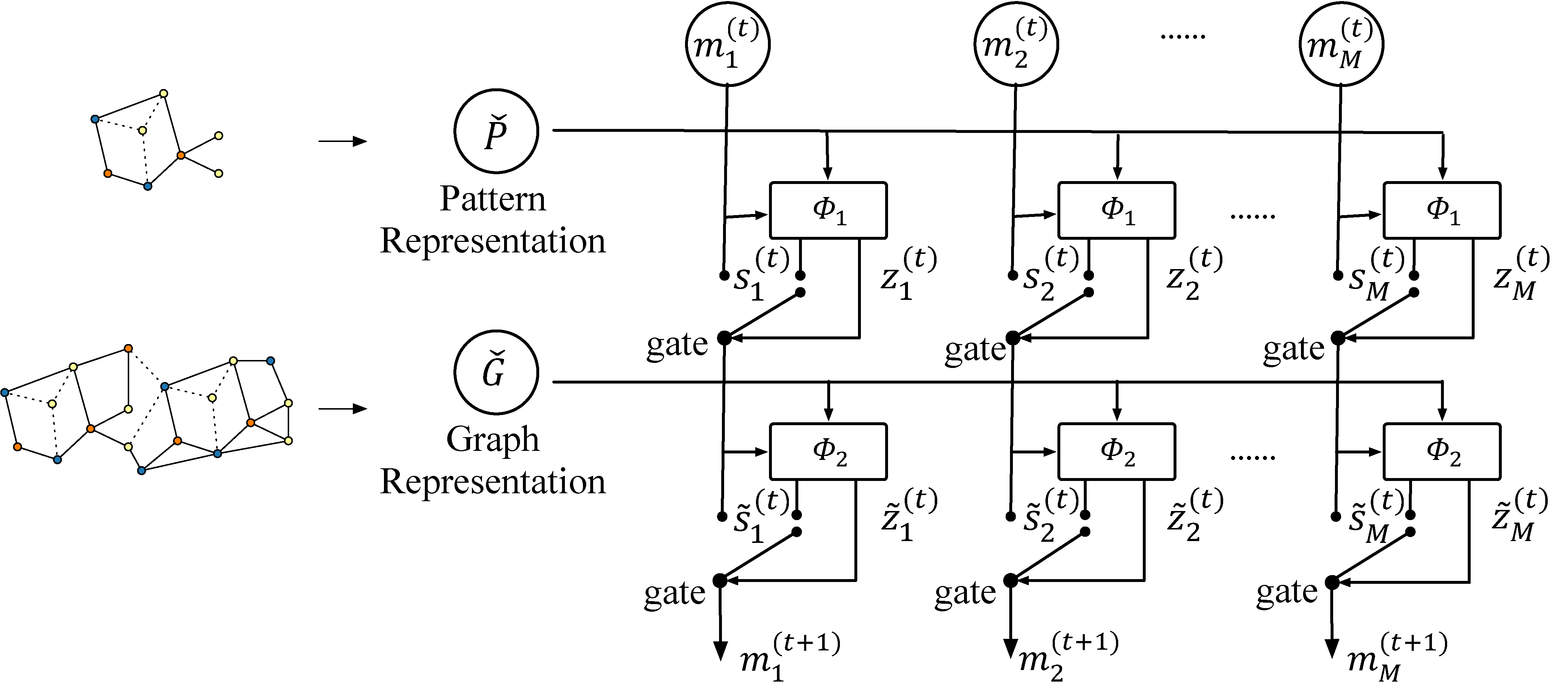
To address the problem of high computational cost in the attention mechanism, we propose the Dynamic Intermedium Attention Memory Network (DIAMNet), using an external memory as an intermedium to attend both the pattern and the graph in order. To make sure that the memory has the knowledge of the pattern while attending the graph and vice-versa, this dynamic memory is designed as a gated recurrent network as shown in Figure 4. Assuming that the memory size is $M$ and we have $T$ recurrent steps, the time complexity is decreased to $\mathcal{O}(T\cdot M\cdot(|\mathcal{E}_{P}|+|\mathcal{E}_{G}|))$ or $\mathcal{O}(T\cdot M\cdot(|\mathcal{V}_{P}|+|\mathcal{V}_{G}|))$, which means the method can be easily applied to large-scale graphs.

The external memory $\bm{M}$ is divided into $M$ blocks $\{\bm{m}_{1},...,\bm{m}_{M}\}$, where $\bm{m}_{j}\in\mathbb{R}^{d}$. At each time step $t$, $\{\bm{m}_{j}\}$ is updated by the pattern and the graph in order via multi-head attention mechanism (Vaswani et al., 2017). Specifically, the update equations of our DIAMNet are given by:

(1) $$\bm{s}_{j}^{(t)} =MultiHead(\bm{m}_{j}^{(t)},\check{\bm{P}},\check{\bm{P}}),$$

(2) $$\bm{z}_{j}^{(t)} =\sigma(\bm{U}_{P}\bm{m}_{j}^{(t)}+\bm{V}_{P}\bm{s}_{j}^{(t)}),$$

(3) $$\overline{\bm{s}}_{j}^{(t)} =\bm{z}_{j}^{(t)}\odot\bm{m}_{j}^{(t)}+(1-\bm{z}_{j}^{(t)})\odot\bm{s}_{j}^{(t)},$$

(4) $$\widetilde{\bm{s}}_{j}^{(t)} =MultiHead(\overline{\bm{s}}_{j}^{(t)},\check{\bm{G}},\check{\bm{G}}),$$

(5) $$\widetilde{\bm{z}}_{j}^{(t)} =\sigma(\bm{U}_{G}\overline{\bm{s}}_{j}^{(t)}+\bm{V}_{G}\widetilde{\bm{s}}_{j}^{(t)}),$$

(6) $$\bm{m}_{j}^{(t+1)} =\widetilde{\bm{z}}_{j}^{(t)}\odot\overline{\bm{s}}_{j}^{(t)}+(1-\widetilde{\bm{z}}_{j}^{(t)})\odot\widetilde{\bm{s}}_{j}^{(t)}.$$

Here $MultiHead$ is the attention method described in (Vaswani et al., 2017), $\sigma$ represents the logistic sigmoid function, $\overline{\bm{s}}_{j}$ is the intermediate state of the $j^{th}$ block of memory that summarizes information from the pattern, and $\widetilde{\bm{s}}$ for information from both the pattern and the graph. $\bm{z}_{j}$ and $\widetilde{\bm{z}}_{j}$ are two gates designed to control the updates on the states in the $j^{th}$ block. $\bm{U}_{P},\bm{V}_{P},\bm{U}_{G},\bm{V}_{G}\in\mathbb{R}^{d\times d}$ are trainable parameters. There are many possible ways to initialize $\bm{M}^{(0)}$, and we discuss the memory initialization in Appendix D.3.

4. Experiments

In this section, we report our major experimental results.

4.1. Datasets

Table 1. Statistics of the datasets. “#” means number, “A.” means average, “M.” means max.

	#Training	#Dev	#Test	A.$(|\mathcal{V}_{G}|)$	A.$(|\mathcal{E}_{G}|)$	M.(Counts)
Small	358,512	44,814	44,814	32.6	76.3	1,024
Large	316,224	39,528	39,528	240.0	560.0	4,096
MUTAG	1,488	1,512	1,512	17.9	39.6	156

In order to train and evaluate our neural models for the subgraph isomorphism counting problem, we need to generate enough graph-pattern data.

Synthetic data

We generate two synthetic datasets, small and large. As there’s no special constraint on the pattern, the pattern generator may produce any connected multigraph without identical edges, i.e., parallel edges with identical label. In contrast, the ground truth numbers of subgraph isomorphisms must be tractable in synthetic data graphs given one pattern. We follow the idea of neighborhood equivalence class (NEC) in TurboISO (Han et al., 2013) to control the necessary conditions of a subgraph isomorphism in the graph generation process. The detailed algorithms are shown in Appendix B. Our graph generator first generates multiple disconnected components, possibly with some subgraph isomorphisms. Then the generator merges these components into a larger graph and ensures that there is no more subgraph isomorphism created during the merging process. Hence, the subgraph isomorphism search can be done over small components in parallel before merging into a large graph. Using the pattern generator and the graph generator above, we can generate many patterns and graphs for neural models. We are interested in follow research questions: whether sequence models and graph models can perform well given limited data, whether their running time is acceptable, whether memory can help models make better predictions even faced with a NP-complete problem, and whether models pre-trained on synthetic data can be transferred to real-life data. To evaluate different neural architectures and different prediction networks, we generate two datasets in different graph scales, with statistics reported in Table 1. There are 187 unique patterns, where 75 patterns belong to the small dataset and 122 patterns belong to the large dataset. Graphs are generated randomly based on these patterns. The generation details are reported in Appendix C.1.

MUTAG

We also generate 24 patterns for 188 graphs on the MUTAG dataset. We use the same pattern generator to generate 24 different heterogenous patterns, and their structures are listed in Appendix C.2. To make the dataset more challenging, graphs in training data, dev data, and test data are disjoint.

4.2. Implementation Details

Instead of directly feeding multi-hot encoding vectors into representation modules, we use two linear layer to separately transform pattern and graph multi-hot vectors to vectors with the predefined hidden size. To improve the efficiency and performance, we also add a filter network to filter out edges or vertices in a graph that are irrelevant to the given pattern before representation modules. The details of this filter network is shown in Section D.1.

4.2.1. Representation Models

In our experiments, we implemented five different representation models: (1) CNN is a 3-layer convolutional layers followed by max-pooling layers. The convolutional kernels are 2,3,4 respectively and strides are 1. The pooling kernels are 2,3,4 and strides are 1. (2) LSTM is a simple 3-layer LSTM model. (3) TXL is a 6-layer Transformer encoder with additional memory. (4) RGCN is a 3-layer RGCN with the block-diagonal-decomposition. We follow the same setting in the original paper to use mean-pooling in the message propagation part. (5) RGIN is a combination of GIN and RGCN: adding a 2-layer MLP after each relational convolutional layer and using the sum aggregator. Residual connections (He et al., 2016) are added to limit the vanish gradient problem.

4.2.2. Interaction Networks

After getting a graph representation $\check{\bm{G}}$ and a pattern representation $\check{\bm{P}}$ from the representation learning modules, we feed them into the following different types of interaction layers for comparison.

Pool: A simple pooling operation is directly applied for the output of neural models for classification or regression. We apply one of sum-pooling, mean-pooling, and max-pooling for $\check{\bm{G}}$ and $\check{\bm{P}}$ to obtain $\check{\bm{g}}$ and $\check{\bm{p}}$, and then send $Concate(\check{\bm{g}},\check{\bm{p}},\check{\bm{g}}-\check{\bm{p}},\check{\bm{g}}\odot\check{\bm{p}})$ with the graph size and the pattern size into the next fully connected (FC) layers.

MemAttn: QA models always use source attention and self-attention to find answers in paragraphs (Hu et al., 2018). One drawback of attention is the computational cost. We consider to use memory for the key and the value. Two gated multi-head attention is applied on $\check{\bm{G}}$ and $\check{\bm{P}}$, which is described in Appendix D.2. Finally, we get the mean-pooled representations for the pattern and the graph and feed the same combination in Pool to the FC layers.

DIAMNet: We compare the performance and efficiency of our DIAMNet proposed in Section 3.3 with above interaction networks. Similarly, we have many initialization strategies in Appendix D.3, but we find mean-pooling is fast and performs well. Finally, we feed the whole memory with size information into the next FC layers. The main difference between DIAMNet and MemAttn is that the memory in DIAMNet is regarded as the query, initialized once and updated $t$ times, but MemAttn initializes memory $2t$ times, takes memory as the key and the value, and updates graph representations $\check{\bm{G}}$ $t$ times.

4.3. Experimental Settings

For fair comparison, we set embedding dimensions, dimensions of all representation models, and the numbers of filters all as 128. The segment size and memory size in TXL are also 64 based on the computational complexity consideration. The length of memory in DIAMNet and MemAttn is fixed to 4 for all experiments. We use the grid search to find the best recurrent steps in MemAttn and DIAMNet. We use the mean squared error (MSE) to train models and choose best models based on the results of dev sets. The optimizer is AdamW (Loshchilov and Hutter, 2019) with a base learning rate of 1e-3 for synthetic data or 1e-4 for real-life data and a weight decay coefficient of 1e-6. To avoid gradient explosion and overfitting, we add gradient clipping and dropout with a dropout rate 0.2. We use $Leaky\_ReLU$ as activation functions in all modules. We use the same representation module with shared parameters to produce representations for both patterns and graphs considering the limited number of patterns.

For the small and large datasets, we first train models on the small and further use curriculum learning (Bengio et al., 2009) on the large. For the MUTAG dataset, we reports results of the best representation model, RGIN, with different numbers of training data. Transfer learning (Pan and Yang, 2010) from synthetic data to MUTAG is also conducted.

Training and evaluating of neural models were finished on NVIDIA V100 GPUs under PyTorch and DGL frameworks. VF2 were finished with 16-core (32 threads) Intel E5-2620v4 CPUs in parallel.

4.4. Evaluation Metrics

As we model this subgraph isomorphism counting problem as a learning problem, we use common metrics in regression tasks, including the root mean square error (RMSE) and the mean absolute error (MAE). In this task, negative predictions are meaningless so that those predictions are regarded as zeros. Two trivial baselines, Zero that always predicts 0 and Avg that always predicts the average count of training data, are also used in comparison.

4.5. Results and Analysis on Synthetic Data

We first report results for the small dataset in Table 2 and results for the large dataset in Table 3. Only the best Pool result is reported for each representation module. In addition to the trivial all-zero and average baselines and other neural network learning based baselines, we are also curious about to what extent our neural models can be faster than traditional searching algorithms. Therefore, we also compare the running time (I/O time excluded). Considering that we use NEC to generate graphs instead of random generation, we compare with VF2 algorithm (Cordella et al., 2004) which does not involve NEC or similar heuristic rules (e.g., rules in VF3 (Carletti et al., 2018)) for fairness. From the experiments, we can draw following observations and conclusions.

Table 2. Results of different models on the small dataset. Time is evaluated on the whole test set.

Models		Test
		RMSE	MAE	Time (sec)
CNN	MaxPool	45.606	8.807	0.808
	MemAttn	30.773	6.066	0.907
	DIAMNet	30.257	5.776	1.198
LSTM	SumPool	32.572	6.353	11.091
	MemAttn	33.497	7.601	11.623
	DIAMNet	32.009	6.013	11.295
TXL	MeanPool	41.102	8.033	8.131
	MemAttn	41.213	7.770	13.531
	DIAMNet	37.897	7.271	13.828
RGCN	SumPool	29.648	5.747	5.400
	MemAttn	25.950	4.973	7.890
	DIAMNet	26.489	4.781	8.435
RGIN	SumPool	20.689	3.657	5.599
	MemAttn	22.067	4.049	8.061
	DIAMNet	20.267	3.632	8.084
Zero		68.457	14.825	-
Avg		66.832	23.633	-
VF2		0.0	0.0	$\sim$110

Comparison of different representation architectures. As shown in Table 2, in general, graph models outperform most of the sequence models. CNN is the worst model for the graph isomorphism counting problem. The code order does not consider the connectivity of adjacent vertices and relevant label information. Hence, convolutional operations and pooling operations cannot extract useful local information but may introduce some noise. From results of the large dataset, we can see that CNN is also worse than others. In fact, we observe CNN always predicts 0 for large graphs. RNN and transformers are widely used in sequence tasks, and LSTM and TXL are advanced variants with memory. We note that LSTM models with different interaction networks are constantly better than TXL. Although memory of LSTM is much smaller than that of TXL, memory of LSTM can somehow memorize all information that has been seen previously but that of TXL is just the representation of the previous segment. In our experiments, the segment size is 64 so that TXL can not learn the global information at a time. The local structure information also misleads TXL, which is consistent with CNN. A longer segment set for TXL may lead to better results, but it will require much more GPU memory and much longer time for training. Graph models perform always better than sequence models. It is not surprising because these graph convolutional operations are designed based on the topology structure. RGIN is much better than RGCN and other sequence models, which shows that MLPs and the sum aggregator are good at vertex representation learning and structure modeling in this task. The mean aggregator can model the distribution of neighbors but the distribution may misguide models (Xu et al., 2019).

Table 3. Results of different models on the large dataset. Time is evaluated on the whole test set.

Model		Test
		RMSE	MAE	Time (sec)
CNN	MaxPool	162.145	27.135	2.334
	MeanAttn	172.568	24.096	2.514
	DIAMNet	125.009	18.642	5.968
LSTM	SumPool	131.778	19.239	16.701
	MeanAttn	130.147	20.997	22.025
	DIAMNet	129.253	19.098	22.511
TXL	MeanPool	161.649	23.952	26.457
	MeanAttn	162.355	24.690	35.169
	DIAMNet	153.588	23.635	35.169
RGCN	SumPool	129.200	18.851	7.639
	MeanAttn	115.981	18.897	12.851
	DIAMNet	110.667	16.760	13.548
RGIN	SumPool	108.183	14.938	7.633
	MeanAttn	111.218	16.494	12.549
	DIAMNet	103.849	14.236	12.798
Zero		219.795	32.868	-
Avg		217.325	57.300	-
VF2		0.0	0.0	$\sim 5\times 10^{3}$

(a) $O_{\mathcal{V}}$, MaxPool

(b) $O_{\mathcal{E}}$, MaxPool

(c) $O_{\mathcal{X}}$, MaxPool

(d) $O_{\mathcal{Y}}$, MaxPool

(e) $O_{\mathcal{V}}$, DIAMNet

(f) $O_{\mathcal{E}}$, DIAMNet

(g) $O_{\mathcal{X}}$, DIAMNet

(h) $O_{\mathcal{Y}}$, DIAMNet

Figure 5. Model behaviors of CNN with MaxPool and CNN with DIAMNet on the small dataset. Here $O_{\mathcal{V}}$ means that the bins on the x-axis are ordered by the size of pattern/graph vertex, $O_{\mathcal{E}}$ by the size of edge, $O_{\mathcal{X}}$ by the size of vertex label, and $O_{\mathcal{Y}}$ by the size of edge label. The orange color refers to the ground truth and the blue color refers to the predictions.

(a) $O_{\mathcal{V}}$, CNN

(b) $O_{\mathcal{E}}$, CNN

(c) $O_{\mathcal{X}}$, CNN

(d) $O_{\mathcal{Y}}$, CNN

(e) $O_{\mathcal{V}}$, RGIN

(f) $O_{\mathcal{E}}$, RGIN

(g) $O_{\mathcal{X}}$, RGIN

(h) $O_{\mathcal{Y}}$, RGIN

Figure 6. Model behaviors of CNN with DIAMNet and RGIN with DIAMNet on the large dataset. Settings are similar to Figure 5.

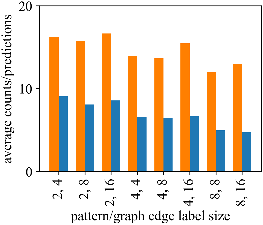
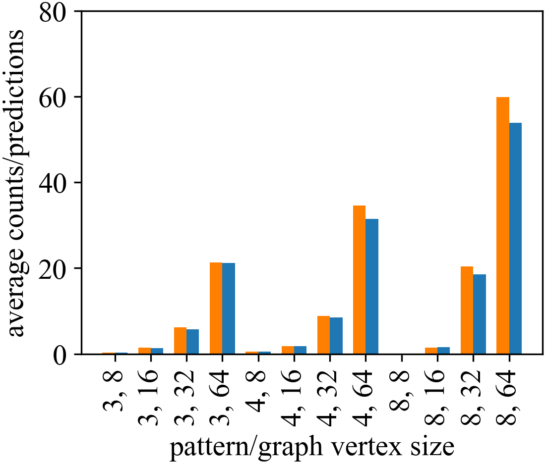
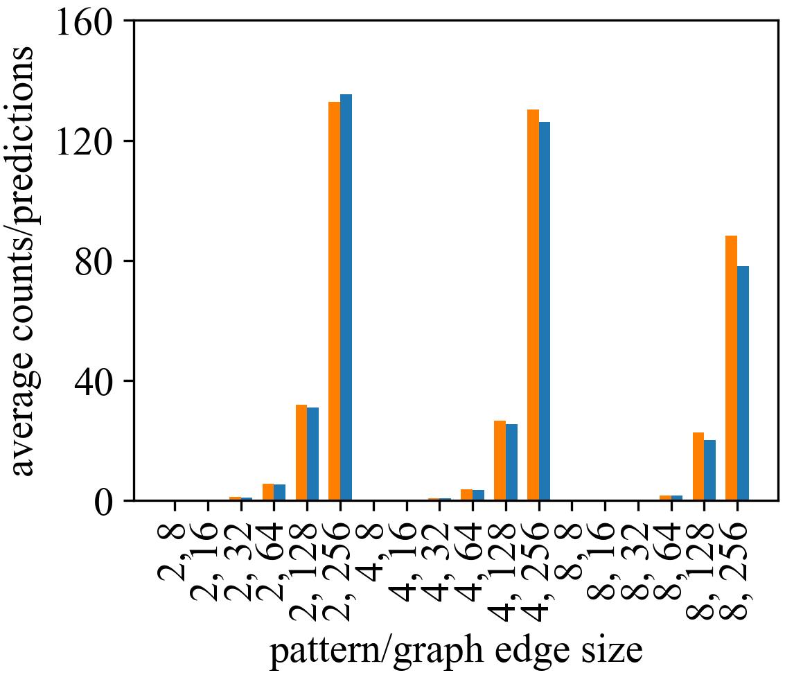
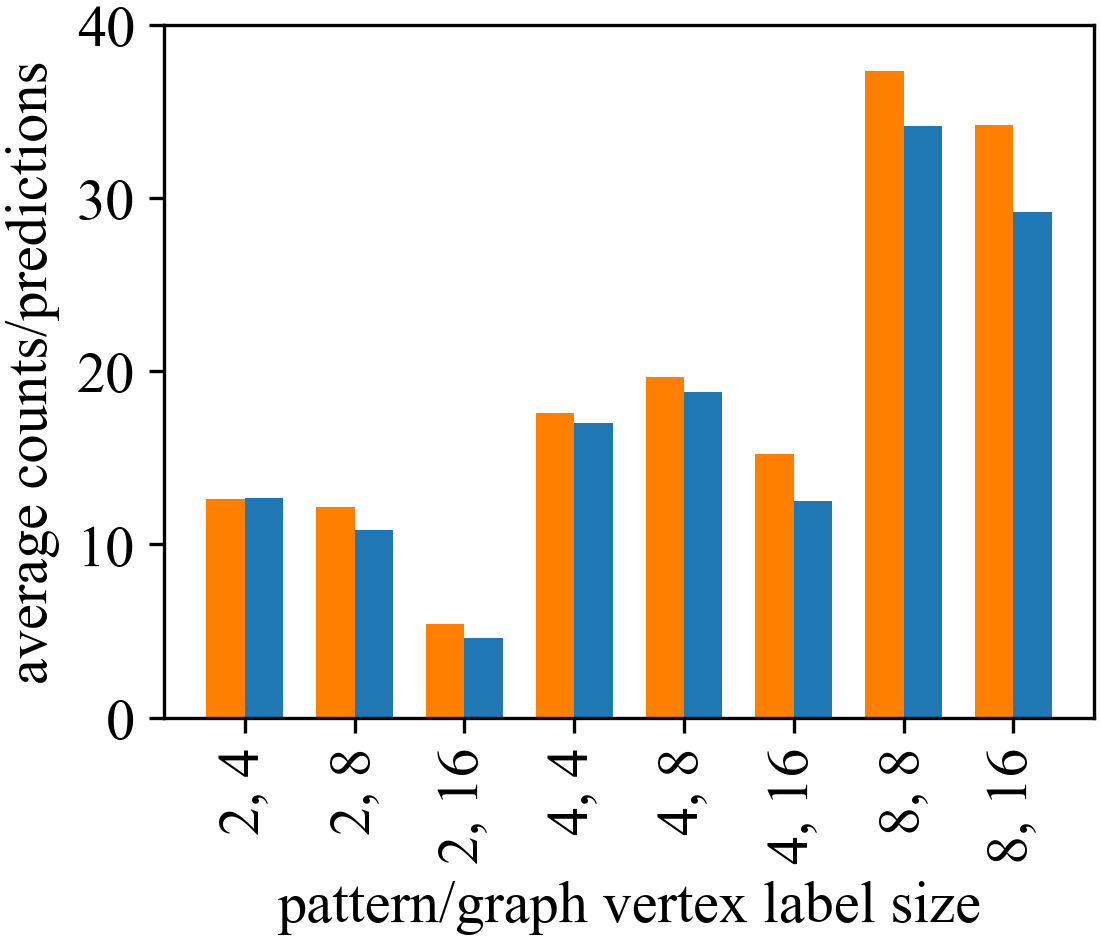
Effectiveness of the memory. Table 2 shows the effectiveness of DIAMNet as the prediction layer. It outperforms the other pooling methods (SumPool, MeanPool, MaxPool) as well as the attention with memory mechanism (MemAttn) for all representation architectures. That means we can use a small extra GPU memory and corresponding computational cost to achieve better results. The memory and computational cost of DIAMNet grows linearly with the size of inputs. The efficiency can not be ignored when models are applied for real-life data with thousands or even millions of vertices and edges. MemAttn can also reduce the quadratic computation cost to linear but its performance is not stable.

Prediction modules based on pooling are in general worse when the representation module is CNN or TXL. This observation indicates that context of the pattern representation should be counted and we need a better way to aggregate information from context. DIAMNet can help extract the context of patterns and graphs even if the representation layer (such as CNN) does not perform very well. Finally, CNN with DIAMNet is the best among sequence models. The local information can be further used to infer in the global level with the help of memory.

Performance on larger graphs. Table 3 shows results of larger-scale graphs. We can find most of the results are consistent to the small dataset. RGIN is still the best representation method in our task and the dynamic memory also works effectively. In terms of the running time, all learning based models are much faster than the traditional VF2 algorithm for subgraph isomorphism counting. Further more, the running time of neural models only increases linearly, making it possible to apply on large-scale real-life data.

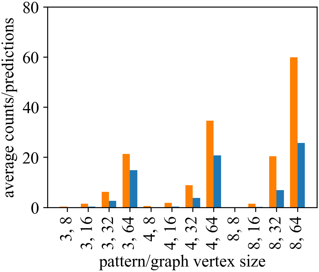
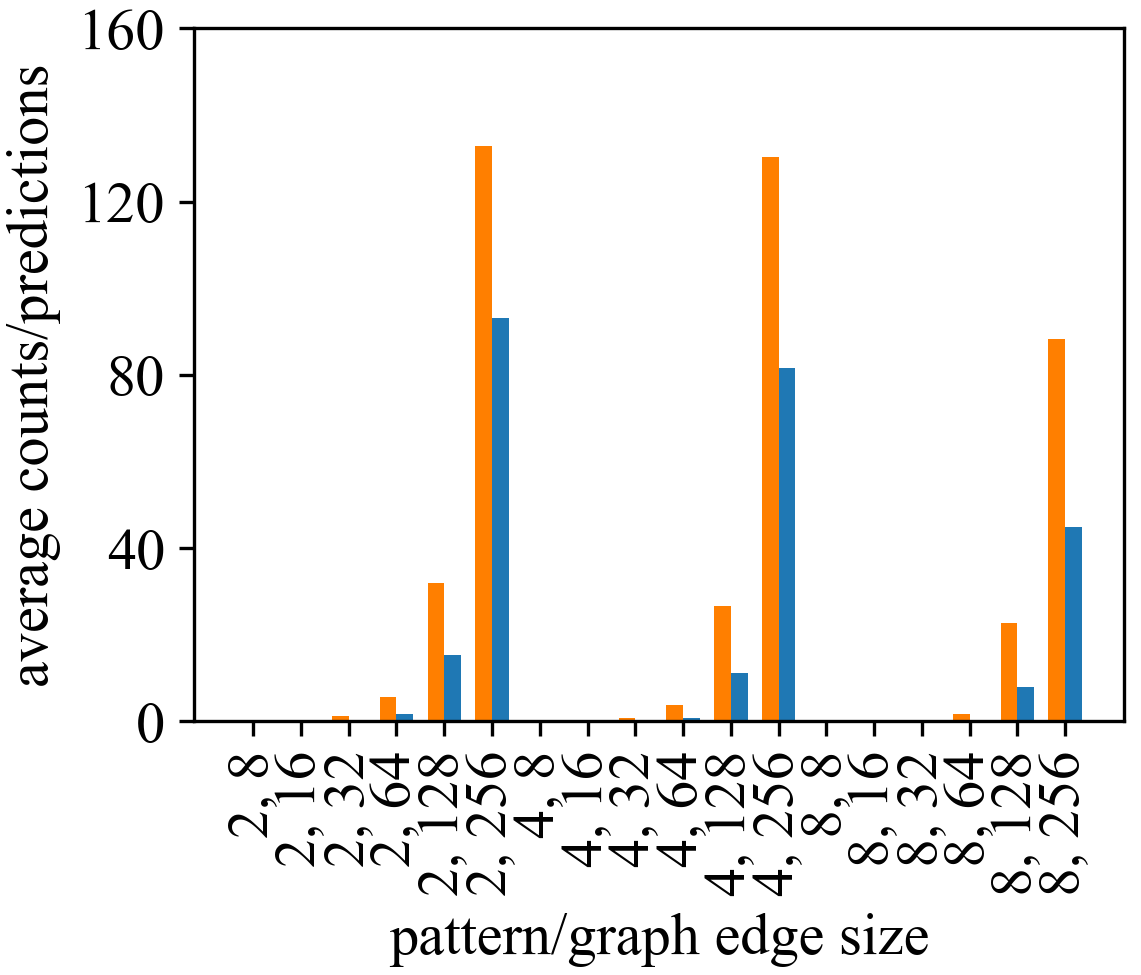
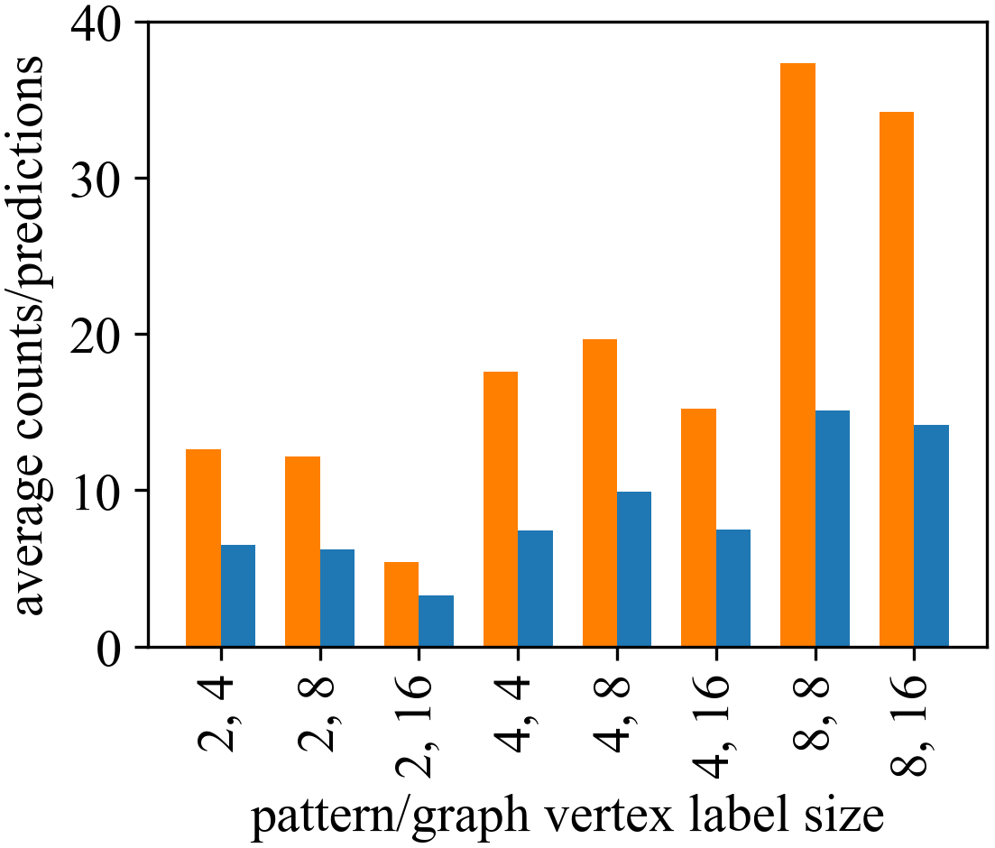
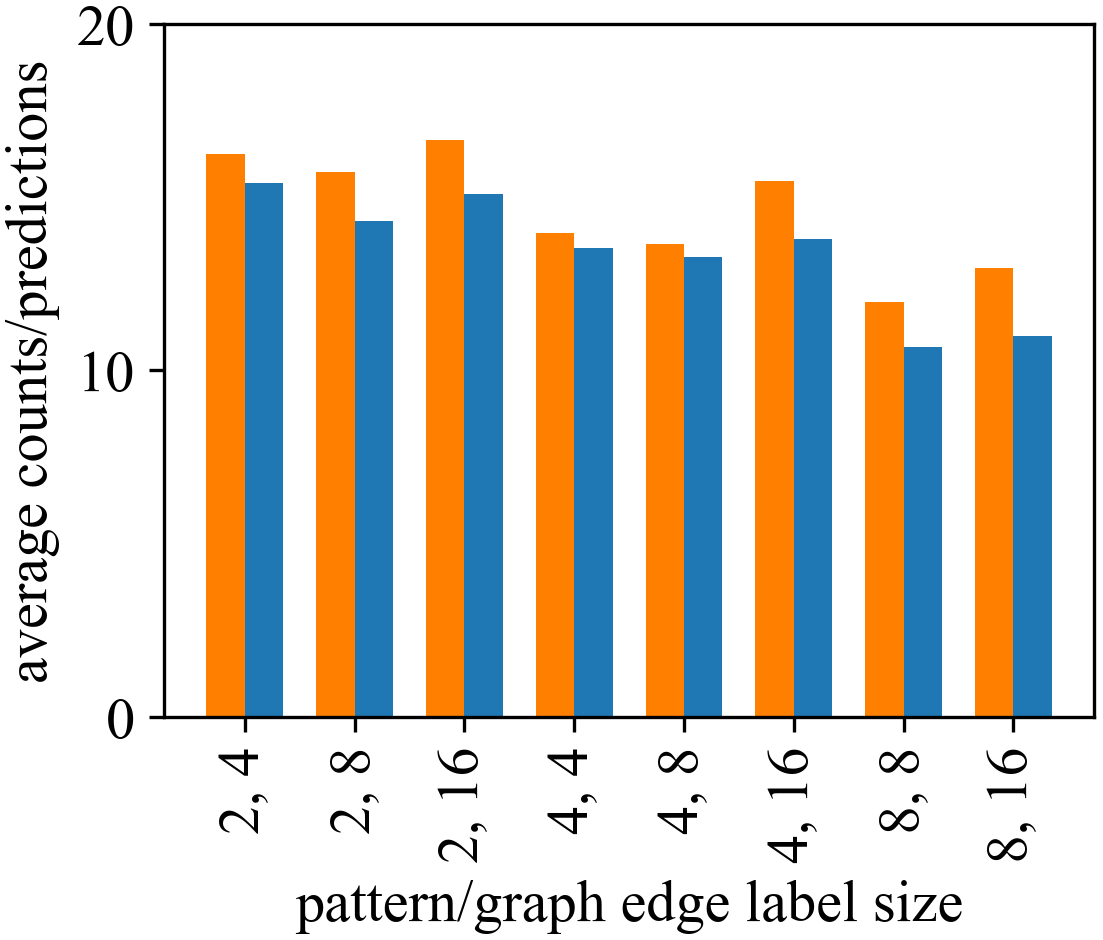
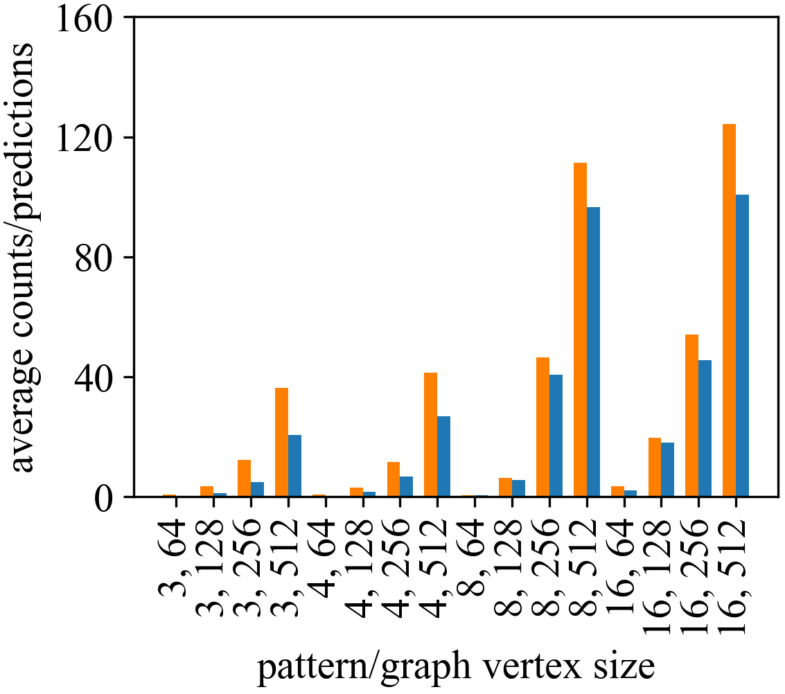
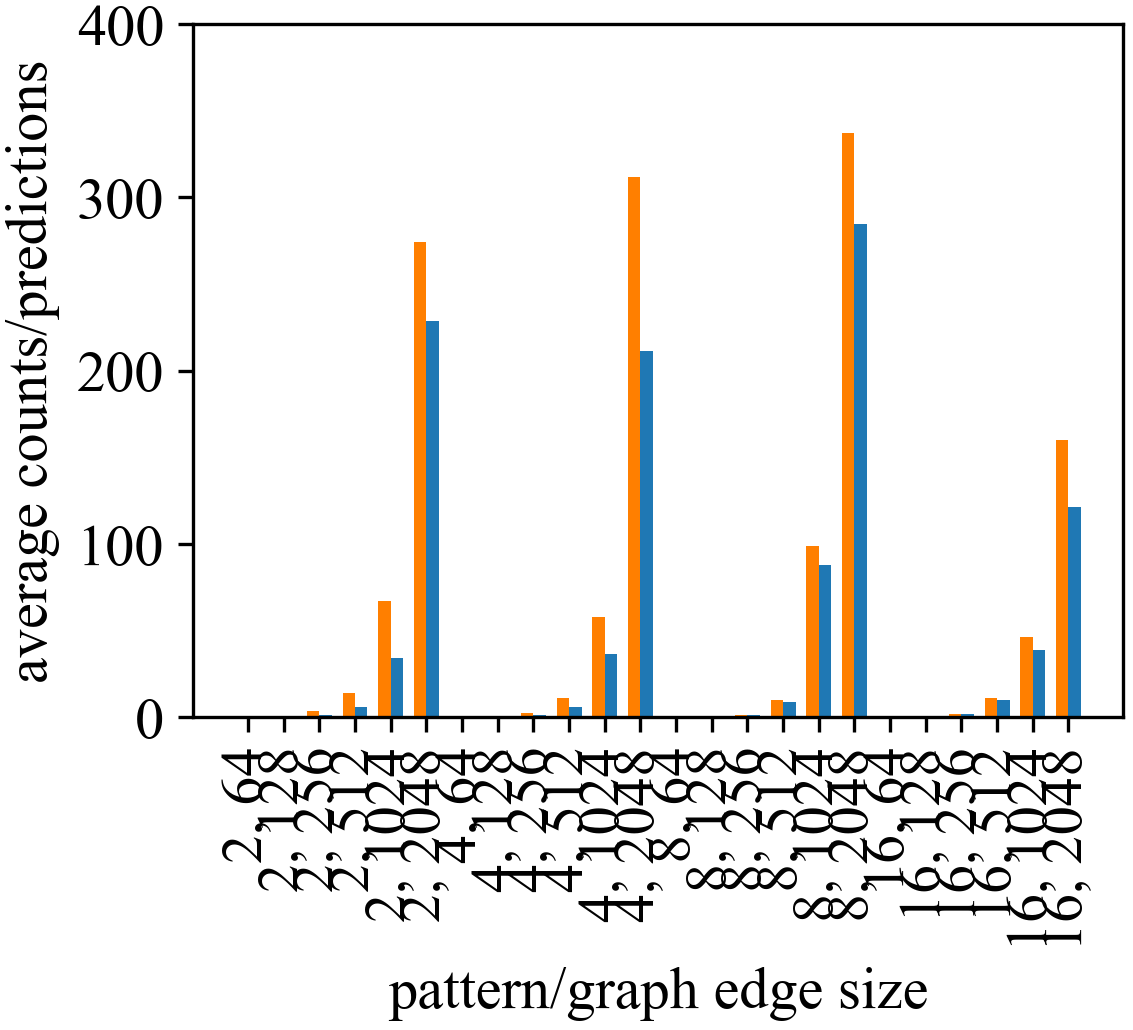
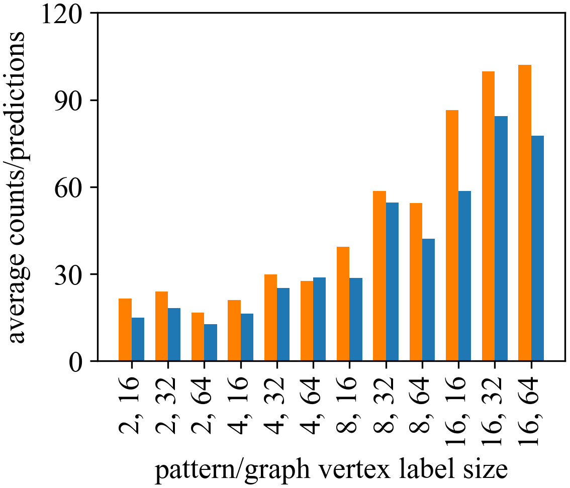
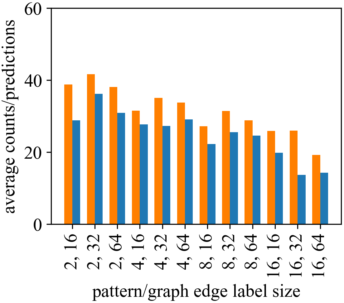
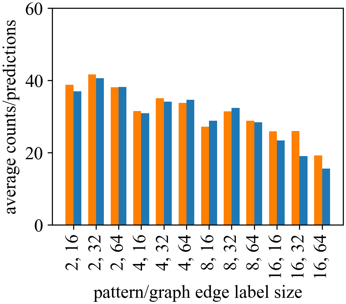
Model behaviors. As shown in Figure 5, the performances of MaxPool and DIAMNet are compared by using the CNN models.

We can find MaxPool always predicts smaller subgraph isomorphisms, while DIAMNet can predict closer numbers even when graphs become large and complex because simple pooling methods will lose much information. On the contrary, the DIAMNet uses small memory to learn which information should be reserved or dropped. In general, our DIAMNet has achieved the better results at most data scales. When bins are ordered by vertex label sizes or edge label sizes, we have the same observation that MaxPool fails when facing complex patterns with more distinct labels but DIAMNet can almost handle all complex situations.

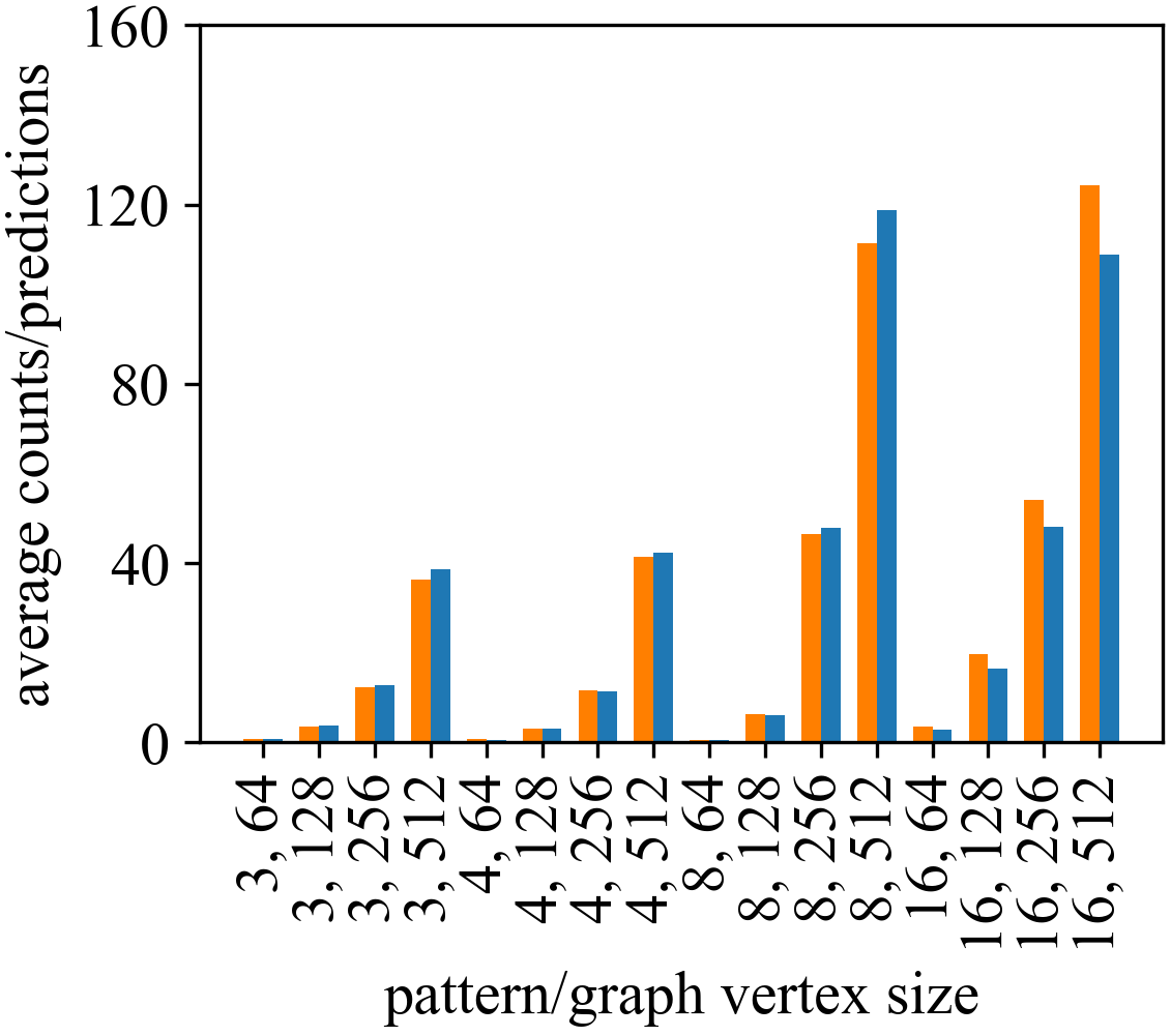
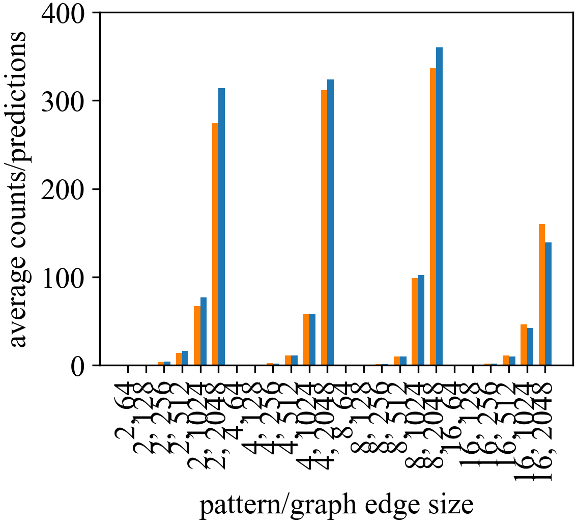
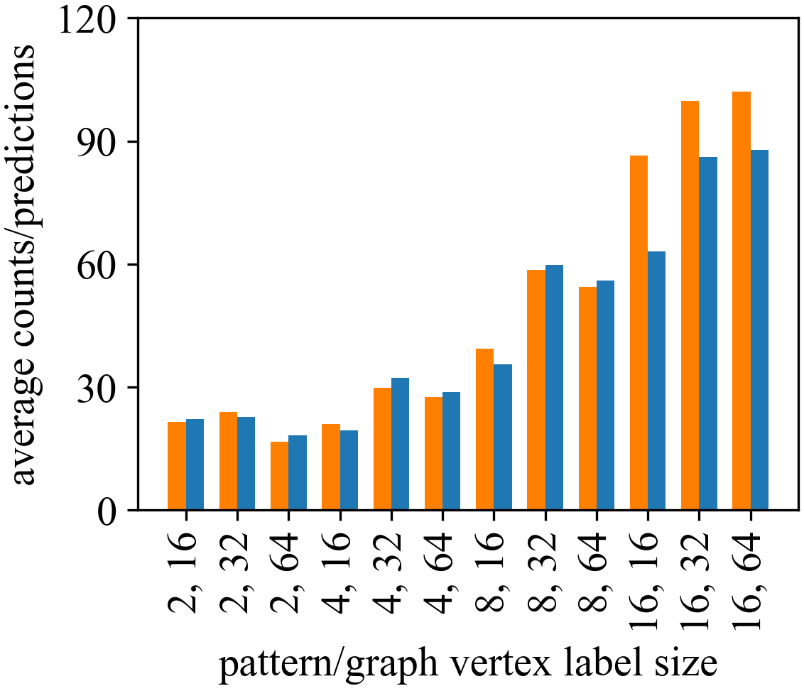
We can also conclude that different representation modules also perform differently from Figure 6. CNN performs worse when the graph size is large (shown in Figure 6(a) and 6(b)) and patterns become complicated (show in Figure 6(c) and 6(d)), which further indicates that CNN only extracts local information and suffers from inference of global information in larger graphs. On the contrary, RGIN with DIAMNet is not affected by edge sizes because it directly learns vertex representations rather than edge representations. Moreover, vertex label sizes and edge label sizes have no apparent ill effects on RGIN, but CNN is seriously affected. Thus it can be seen that simply convolutional and pooling operations with little topology information are not suitable for this task.

4.6. Transfer Learning on MUTAG

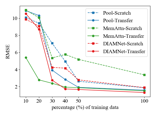
For the MUTAG data, We feed different numbers of training pairs to RGIN with different interaction networks and try transfer learning by fine-tuning models trained on the small dataset. Results are shown in Figure 7. The performance gap between models from scratch and models by transfer learning cannot be neglected when the training data are not enough. With the help of transfer learning, the fine-tuned RGIN with any interaction modules can reduce RMSE smaller than 1.588 while the RMSE of the best model from scratch is still around 1.884. When limited training data are given, all models perform not well except the MemAttn-Transfer. We can observe huge improvements by transfer learning when providing 30%-40% training data. DIAMNet-Transfer becomes the best afterwards and finally achieves 1.307 RMSE and 0.440 MAE. It is worth noticing that test graphs never appear in the training data on the MUTAG, which indicates that our learning to count framework and algorithms are promising to handle large-scale real world graphs in the future.

Figure 7. Results of RGIN based models on the MUTAG dataset. Dashed lines are results of models trained from scratch while solid lines are results by transfer learning. The Zero and the Avg result in 19.384 and 17.754 RMSE respectively when 100% training data are used.

5. Related Work

Subgraph Isomophism Problems. Given a pattern graph and a data graph, the subgraph isomorphism search aims to find all occurrences of the pattern in the data graph with bijection mapping functions. Subgraph isomorphism is an NP-complete problem among different types of graph matching problems (monomorphism, isomorphism, and subgraph isomorphism). Most subgraph isomorphism algorithms are based on backtracking. They first obtain a series of candidate vertices and update a mapping table, then recursively revoke their own subgraph searching functions to match one vertex or one edge at a time. Ullmann’s algorithm (Ullmann, 1976), VF2 (Cordella et al., 2004), and GraphQL (He and Singh, 2008) belong to this type of algorithms. However, it is still hard to perform search when either the pattern or the data graph grows since the search space grows exponentially as well. Some other algorithms are designed based on graph-index, such as gIndex (Yan et al., 2004), which can be used as filters to prune out many unnecessary graphs. However, graph-index based algorithms have a problem that the time and space in indexing also increase exponentially with the growth of the graphs (Sun et al., 2012). TurboISO (Han et al., 2013) and VF3 (Carletti et al., 2018) add some weak rules to find candidate subregions and then call the recursive match procedure on subregions. These weak rules can significantly reduce the searching space in most cases. In addition, there are also some approximation techniques (Tsourakakis, 2008; Eden et al., 2017) for triangle counting but they are hard to generalized to large patterns. Random walks are also used to count subgraph isomorphisms (Teixeira et al., 2018; Wang et al., 2014) but the cost and errors are still issues. Graph simulation (Fan et al., 2010; Ma et al., 2014) is another way to find subgraph isomorphisms in cubic-time, but researchers require to rectify the failure of topology capturing and false or fake matches.

Graph Representation Learning. Graph (or network) representation learning can be directly learning an embedding vector of each graph node (Perozzi et al., 2014; Tang et al., 2015; Grover and Leskovec, 2016). This approach is not easy to generalize to unseen nodes. On the other hand, graph neural networks (GNNs) (Battaglia et al., 2018) provide a solution to representation learning for nodes which can be generalized to new graphs and unseen nodes. Many graph neural networks have been proposed since 2005 (Gori et al., 2005; Scarselli et al., 2005) but rapidly developed in recent years. Most of them focus on generalizing the idea of convolutional neural networks for general graph data structures (Niepert et al., 2016; Kipf and Welling, 2017; Hamilton et al., 2017b; Velickovic et al., 2018) or relational graph structures with multiple types of relations (Schlichtkrull et al., 2018). More recently, (Xu et al., 2019) propose a graph isomorphism network (GIN) and show its discriminative power. Others use the idea of recurrent neural networks (RNNs) which are originally proposed to deal with sequence data to work with graph data (Li et al., 2016; You et al., 2018). Interestingly, with external memory, sequence models can work well on complicated tasks such as language modeling (Sukhbaatar et al., 2015; Kumar et al., 2016) and shortest path finding on graphs (Graves et al., 2016). There is another branch of research called graph kernels (Vishwanathan et al., 2010; Shervashidze et al., 2011; Yanardag and Vishwanathan, 2015; Togninalli et al., 2019; Chen et al., 2019) which also convert graph isomorphism to a similarity learning problem. However, they usually work on small graphs and do not focus on subgraph isomorphism identification or counting problems.

6. Conclusions

In this paper, we study the challenging subgraph isomorphism counting problem. With the help of deep graph representation learning, we are able to convert the NP-complete problem to a learning based problem. Then we can use learned models to predict the subgraph isomorphism counts in polynomial time. We build two synthetic datasets to evaluate different representation learning models and global inference models. Results show that learning based method is a promising direction for subgraph isomorphism detection and counting and our dynamic intermedium attention memory network indeed help the global inference.

Acknowledgements. This paper was supported by the Early Career Scheme (ECS, No. 26206717) and the Research Impact Fund (RIF, No. R6020-19) from the Research Grants Council (RGC) in Hong Kong, and the Gift Fund from Huawei Noah’s Ark Lab.

Appendix A Lexicographic Order of Codes

The lexicographic order is a linear order defined as follows:

If $A=(a_{0},a_{1},\cdots,a_{m})$ and $B=(b_{0},b_{1},\cdots,b_{n})$ are the codes, then $A\leq B$ iff either of the following is true:

1. $\exists t,0\leq t\leq min(m,n),\forall k<t,a_{k}=b_{k},a_{t}\prec_{e}b_{t}$,

2. $\forall 0\leq k\leq m,a_{k}=b_{k},\text{ and }n\geq m$.

In our setting, $a_{i}=(u_{a_{i}},v_{a_{i}},\mathcal{X}(u_{a_{i}}),y_{a_{i}},\mathcal{X}(v_{a_{i}}))\prec_{e}\\ b_{j}=(u_{b_{j}},v_{b_{j}},\mathcal{X}(u_{b_{j}}),y_{b_{j}},\mathcal{X}(v_{b_{j}}))$ iff one of the following is true:

1. $u_{a_{i}}<u_{b_{j}}$,

2. $u_{a_{i}}=u_{b_{j}},v_{a_{i}}<v_{b_{j}}$,

3. $u_{a_{i}}=u_{b_{j}},v_{a_{i}}=v_{b_{j}},y_{a_{i}}<y_{b_{j}}$.

Appendix B Pattern Generator and Graph Generator

As proposed in Section 4.1, two generators are required to generate datasets. The algorithm about the pattern generator is shown in Algorithm 1. The algorithm first uniformly generates a directed tree. Then it adds the remaining edges with random labels. Vertex labels and edge labels are also uniformly generated but each label is required to appear at least once. Algorithm 2 shows the process of graph generation. Two hyperparameters control the density of subisomorphisms: (1) $\alpha\in[0,1]$ decides the probability of adding subisomorphisms rather than random edges; (2) $\beta\in\mathbb{N}^{+}$ is the parameter of Dirichlet distribution to sample sizes of components. After generating several directed trees and satisfying the vertex number requirement, the algorithm starts to add remaining edges. It can add edges in one component and try to add subgraph isomorphisms, or it can randomly add edges between two components or in one component. The following merge subroutine aims to merge these components into a large graph. Shuffling is also required to make datasets hard to be hacked. The search of subisomorphisms in the whole graph is equivalent to the search in components respectively because edges between any two components do not satisfy the necessary conditions.

Algorithm 1 Pattern Generator.

1:the number of vertices $N_{v}$, the number of edges $N_{e}$, the number of vertex labels $L_{v}$, the number of edge labels $L_{e}$.

2:$\mathcal{P}$ := GenerateDirectedTree($N_{v}$)

3:AssignNodesLabels($\mathcal{P}$, $L_{v}$)

4:AddRandomEdges($\mathcal{P}$, $\mathcal{P}$, $null$, $N_{e}-N_{v}+1$)

5:AssignEdgesLabels($\mathcal{P}$, $L_{e}$)

6:the generated pattern $\mathcal{P}$

Algorithm 2 Graph Generator.

1:a pattern $\mathcal{P}$, the number of vertices $N_{v}$, the number of edges $N_{e}$, the number of vertex labels $L_{v}$, the number of edge labels $L_{e}$, hyperparameters $\alpha$ and $\beta$.

2:$Ns$ := DirichletSampling($N_{v}$, $\beta$)

3:$\mathcal{G}s$ := $\{\}$

4:$d_{e}$ := $N_{e}$

5:for each $n$ in $Ns$ do

6:    $g$ := GenerateDirectedTree($n$)

7:    AssignNodesLabels($g$, $n$)

8:    AssignEdgesLabels($g$, $n-1$)

9:    $\mathcal{G}s$ := $\mathcal{G}s+\{g\}$

10:    $d_{e}$ := $d_{e}-n+1$

11:end for

12:$T_{p}$ := RewriteNECTree($\mathcal{P}$)

13:$N_{e,\mathcal{P}}$ := EdgeCount($\mathcal{P}$)

14:while $d_{e}>0$ do

15:    $g_{1}$, $g_{2}$ = RandomPick($\mathcal{G}s$, 2) $\triangleright$ Pick two components randomly

16:    $r$ = RandomNum(0, 1)

17:    if $d_{e}<N_{e,\mathcal{P}}$ then

18:        $d_{e}$ := $d_{e}$ - AddRandomEdges($g_{1}$, $g_{2}$, $T_{p}$, $d_{e}$) $\triangleright$ Add $d_{e}$ edges between $g_{1}$ and $g_{2}$

19:    else

20:        if $r<\alpha$ then

21:           $d_{e}$ := $d_{e}$ - AddPatterns($g_{1}$, $\mathcal{P}$) $\triangleright$ Add necessary edges in $g_{1}$ to add patterns

22:        else

23:           $d_{e}$ := $d_{e}$ - AddRandomEdges($g_{1}$, $g_{2}$, $T_{p}$, $N_{e,\mathcal{P}}$)

24:        end if

25:    end if

26:end while

27:$\mathcal{G}$, $f$ := MergeComponents($\mathcal{G}s$) $\triangleright$ $f$ is the graph id mapping

28:$\mathcal{G}$, $f^{\prime}$ := ShuffleGraph($\mathcal{G}$) $\triangleright$ $f^{\prime}$ is the shuffled graph id mapping

29:$\mathcal{I}s$ := $\{\}$

30:for each $g$ in $\mathcal{G}s$ do

31:    $Is$ := SearchSubIsomorphisms($g$, $\mathcal{P}$)

32:    for each $I$ in $Is$ do

33:        $I$ := UpdateID($I$, $f$, $f^{\prime}$)

34:        $\mathcal{I}s$ := $\mathcal{I}s+\{I\}$

35:    end for

36:end for

37:the generated graph $\mathcal{G}$, the subgraph isomorphisms $\mathcal{I}s$

In Algorithm 1 and Algorithm 2, the function AddRandomEdges adds required edges from one component to the other without generating new subgraph isomorphisms. The two component can also be the same one, which means to add in one component. The NEC tree is utilized in TurboISO (Han et al., 2013) to explore the candidate region for further matching. It takes $\mathcal{O}(|\mathcal{V}_{p}|^{2})$ time but can significant reduce the searching space in the data graph. It records the equivalence classes and necessary conditions of the pattern. We make sure edges between two components dissatisfy necessary conditions in the NEC tree when adding random edges between them. This data structure and this idea help us to generate more data and search subisomorphisms compared with random generation and traditional subgraph isomorphism searching.

Appendix C Details of Datasets

C.1. Details of Synthetic Datasets

We can generate as many examples as possible using two graph generators. However, we limit the numbers of training, dev, and test examples whether learning based models can generalize to new unseen examples. Pattern and data graphs in different scales have been generated. Parameters for two generators and constraints are listed in Table 4. Two constraints are added to make this task easier. The average degree constraint ($\frac{N_{e}}{N_{v}}\leq 4$) is used to keep graphs not so dense, and the subisomorphism counting constraints ($\{c\in\mathbb{N}|c\leq 1,024\}$ for small, $\{c\in\mathbb{N}|c\leq 4,096\}$ for large) ensure the difficulty of two datasets are different.

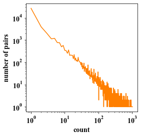
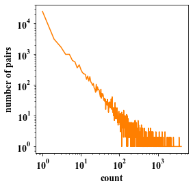
We generated data with an 8-core (16 threads) Intel E5-2620v4 CPU in parallel. The distributions of countings of two datasets are shown in Figure 8. From the figure we can see that both datasets follow the long tail distributions.

Table 4. Parameters and constraints for two datasets

	Hyperparameters	small	large
Pattern	$N_{v}$	{3, 4, 8}	{3, 4, 8, 16}
	$N_{e}$	{2, 4, 8}	{2, 4, 8, 16}
	$L_{v}$	{2, 4, 8}	{2, 4, 8, 16}
	$L_{e}$	{2, 4, 8}	{2, 4, 8, 16}
Graph	$N_{v}$	{8, 16, 32, 64}	{64, 128, 256, 512}
	$N_{e}$	{8, 16, $\cdots$, 256}	{64, 128, $\cdots$, 2,048}
	$L_{v}$	{4, 8, 16}	{16, 32, 64}
	$L_{e}$	{4, 8, 16}	{16, 32, 64}
	$\alpha$	{0.2, $\cdots$, 0.8}	{0.05, 0.1, 0.15}
	$\beta$	{512}	{512}

(a) Test data distribution of the small dataset.

(b) Test data distribution of the large dataset.

Figure 8. Subgraph isomorphism counting distributions of two datasets.

C.2. Details of MUTAG Dataset

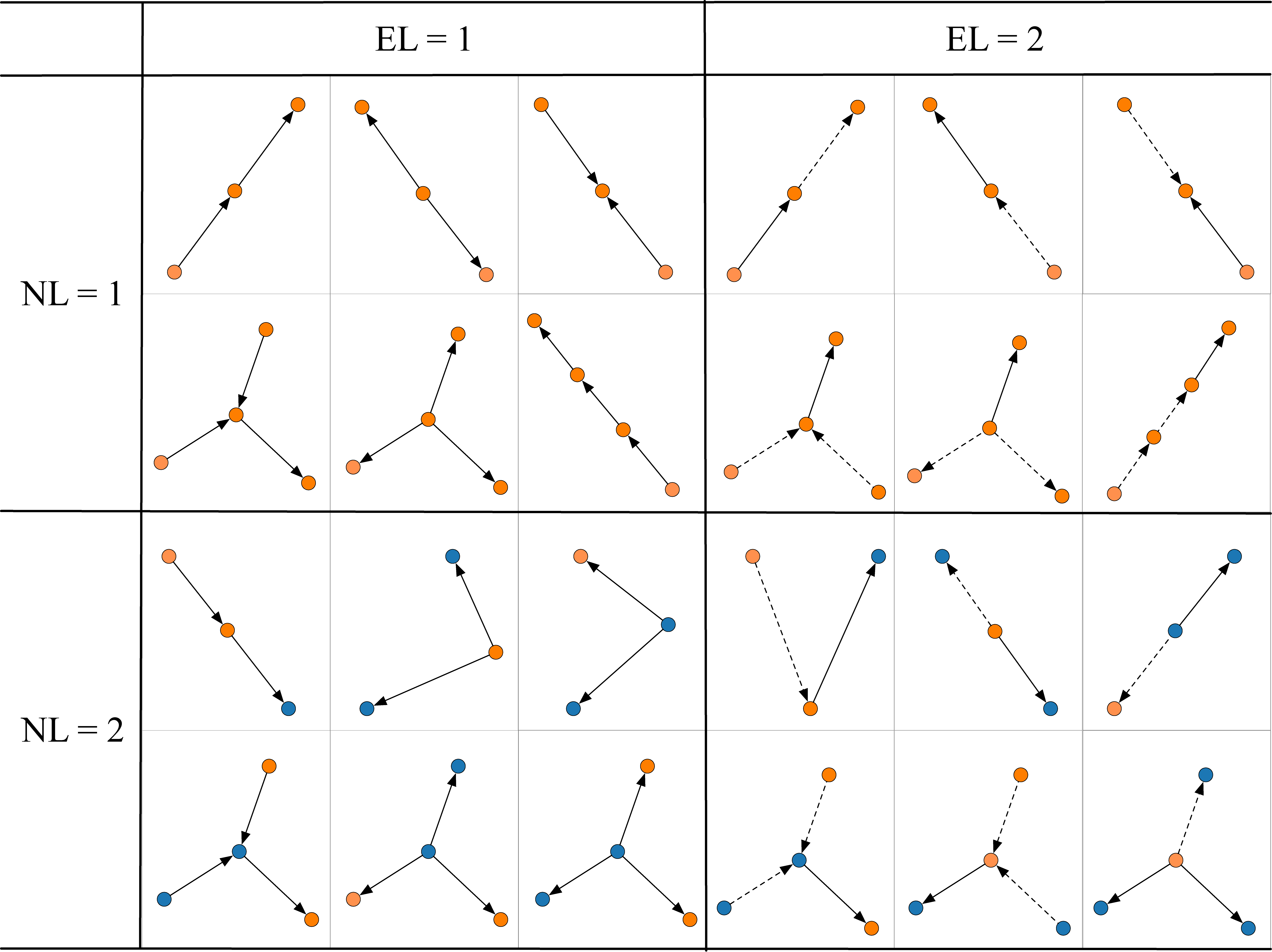
MUTAG dataset contains 188 mutagenic compound graphs. We split 188 graphs as 62 training graphs, 63 validation graphs and 63 test graphs. We use the pattern generator in Appendix B to generate 24 different patterns and finally construct 4,512 graph-pattern pairs (1,488 training pairs, 1,512 validation pairs and 1,512 test pairs). The detailed pattern structures are shown in Figure 9.

Appendix D More Implementation Details

In this section, we provide more implementation details other than the representation architectures and the DIAMNet modules.

D.1. Filter Network

Intuitively, not all vertices and edges in graphs can match certain subisomorphisms so we simply add a FilterNet to adjust graph encoding as follows:

(7) $$\overline{\bm{p}} =MaxPool(\bm{p}),$$

(8) $$\widehat{\bm{G}} =\bm{G}\bm{W}_{G}^{\top},$$

(9) $$\bm{f}_{i} =\sigma(\bm{W}_{F}(\widehat{\bm{G}}_{i,:}\odot\overline{\bm{p}})),$$

(10) $$\bm{G}_{i,:} =\bm{f}_{i}\odot\bm{G}_{i,:},$$

where $\widehat{\bm{G}}$ is the graph representation in the pattern space, $\sigma$ is the sigmoid function, $f_{i}$ is the gate that decides to filter the $j^{th}$ vertex or the $j^{th}$ edge, $\bm{W}_{G}\in\mathbb{R}^{d_{p}\times d_{g}}$ and $\bm{W}_{F}\in\mathbb{R}^{1\times d_{p}}$ are trainable. Thanks to the multi-hot encoding, We can simply use Eq. (7) to accumulate label information of patterns. After this filter layer, only relevant parts of the graphs will be passed to the next representation layer.

Figure 9. 24 different patterns in the MUTAG dataset.

D.2. MemAttn

To address the quadratic-cost problem, we involve memory for the key and the value and do the dot-product between the query and the memory. We initialize $\check{\bm{G}}^{(0)}$ as $\check{\bm{G}}$ and update $t$ times. The details are listed as follows:

(11) $$\bm{M}^{(t)} =MemInit(\check{\bm{P}}),$$

(12) $$\bm{s}_{j}^{(t)} =MultiHead(\check{\bm{g}}_{j}^{(t)},\bm{M}^{(t)},\bm{M}^{(t)}),$$

(13) $$\bm{z}_{j}^{(t)} =\sigma(\bm{U}_{P}\check{\bm{g}}_{j}^{(t)}+\bm{V}_{P}\bm{s}_{j}^{(t)}),$$

(14) $$\overline{\bm{s}}_{j}^{(t)} =\bm{z}_{j}^{(t)}\odot\check{\bm{g}}_{j}^{(t)}+(1-\bm{z}_{j}^{(t)})\odot\bm{s}_{j}^{(t)},$$

(15) $$\overline{\bm{M}}^{(t)} =MemInit(\overline{\bm{S}}^{(t)}),$$

(16) $$\widetilde{\bm{s}}_{j}^{(t)} =MultiHead(\overline{\bm{s}}_{j}^{(t)},\overline{\bm{M}}^{(t)},\overline{\bm{M}}^{(t)}),$$

(17) $$\widetilde{\bm{z}}_{j}^{(t)} =\sigma(\bm{U}_{S}\overline{\bm{s}}_{j}^{(t)}+\bm{V}_{S}\widetilde{\bm{s}}_{j}^{(t)}),$$

(18) $$\check{\bm{g}}_{j}^{(t+1)} =\widetilde{\bm{z}}_{j}^{(t)}\odot\overline{\bm{s}}_{j}^{(t)}+(1-\widetilde{\bm{z}}_{j}^{(t)})\odot\widetilde{\bm{s}}_{j}^{(t)}.$$

There are many ways to initialize memory, and we discuss briefly in Appendix D.3. In experiments, we simply choose to initialize by mean-pooling.

D.3. Memory Initialization

There are many ways to initialize the memory $\bm{M}=\{\bm{m}_{1},\cdots,\bm{m}_{M}\}$ given an input $\bm{L}=\{\bm{l}_{1},\cdots,\bm{l}_{L}\}$. In experiments, we simply initialize $\bm{m}_{i}$ by

(19) $$s =\lfloor\frac{L}{M}\rfloor,$$

(20) $$k =L-(M-1)\cdot s,$$

(21) $$\bm{m}_{i} =MeanPool(\{\bm{l}_{i\cdot s},\cdots,\bm{l}_{i\cdot s+k-1}\}),$$

where $s$ is the stride and $k$ is the kernel size. Simply splitting the padded input with length $M\cdot\lceil\frac{L}{M}\rceil$ is also supposed to work well. It is easy to replace the mean-pooling with max-pooling and sum-pooling. Interestingly, we can also use self-attention for $\{\bm{l}_{i\cdot s},\cdots,\bm{l}_{i\cdot s+k-1}\}$ to get a better memory block $\bm{m}_{i}$. However, self-attention makes the initialization no faster than $\mathcal{O}(L^{1.5})$. One further work is to design hashing and selection to help memory memorize better global and local structure information of $\bm{L}$, such as nodes with same vertex labels storing in the same memory block.

References

- (1)
- Alon et al. (2008) Noga Alon, Phuong Dao, Iman Hajirasouliha, Fereydoun Hormozdiari, and Süleyman Cenk Sahinalp. 2008. Biomolecular network motif counting and discovery by color coding. In ISMB. 241–249.
- Bahdanau et al. (2015) Dzmitry Bahdanau, Kyunghyun Cho, and Yoshua Bengio. 2015. Neural Machine Translation by Jointly Learning to Align and Translate. In ICLR.
- Battaglia et al. (2018) Peter W. Battaglia, Jessica B. Hamrick, Victor Bapst, Alvaro Sanchez-Gonzalez, Vinícius Flores Zambaldi, Mateusz Malinowski, Andrea Tacchetti, David Raposo, Adam Santoro, Ryan Faulkner, Çaglar Gülçehre, H. Francis Song, Andrew J. Ballard, Justin Gilmer, George E. Dahl, Ashish Vaswani, Kelsey R. Allen, Charles Nash, Victoria Langston, Chris Dyer, Nicolas Heess, Daan Wierstra, Pushmeet Kohli, Matthew Botvinick, Oriol Vinyals, Yujia Li, and Razvan Pascanu. 2018. Relational inductive biases, deep learning, and graph networks. CoRR abs/1806.01261 (2018).
- Bengio et al. (2009) Yoshua Bengio, Jérôme Louradour, Ronan Collobert, and Jason Weston. 2009. Curriculum learning. In ICML. 41–48.
- Carletti et al. (2018) Vincenzo Carletti, Pasquale Foggia, Alessia Saggese, and Mario Vento. 2018. Challenging the Time Complexity of Exact Subgraph Isomorphism for Huge and Dense Graphs with VF3. PAMI 40, 4 (2018), 804–818.
- Chen et al. (2019) Zhengdao Chen, Soledad Villar, Lei Chen, and Joan Bruna. 2019. On the equivalence between graph isomorphism testing and function approximation with GNNs. In NeurIPS. 15868–15876.
- Cho et al. (2014) Kyunghyun Cho, Bart van Merrienboer, Çaglar Gülçehre, Dzmitry Bahdanau, Fethi Bougares, Holger Schwenk, and Yoshua Bengio. 2014. Learning Phrase Representations using RNN Encoder-Decoder for Statistical Machine Translation. In EMNLP. 1724–1734.
- Cordella et al. (2004) Luigi P. Cordella, Pasquale Foggia, Carlo Sansone, and Mario Vento. 2004. A (Sub)Graph Isomorphism Algorithm for Matching Large Graphs. PAMI 26, 10 (2004), 1367–1372.
- Dai et al. (2019) Zihang Dai, Zhilin Yang, Yiming Yang, Jaime G. Carbonell, Quoc Viet Le, and Ruslan Salakhutdinov. 2019. Transformer-XL: Attentive Language Models beyond a Fixed-Length Context. In ACL. 2978–2988.
- Eden et al. (2017) Talya Eden, Amit Levi, Dana Ron, and C. Seshadhri. 2017. Approximately Counting Triangles in Sublinear Time. SIAM J. Comput. 46, 5 (2017), 1603–1646.
- Fan et al. (2019) Changjun Fan, Li Zeng, Yuhui Ding, Muhao Chen, Yizhou Sun, and Zhong Liu. 2019. Learning to Identify High Betweenness Centrality Nodes from Scratch: A Novel Graph Neural Network Approach. In CIKM. 559–568.
- Fan et al. (2010) Wenfei Fan, Jianzhong Li, Shuai Ma, Nan Tang, Yinghui Wu, and Yunpeng Wu. 2010. Graph Pattern Matching: From Intractable to Polynomial Time. VLDB 3, 1 (2010), 264–275.
- Fang et al. (2016) Yuan Fang, Wenqing Lin, Vincent Wenchen Zheng, Min Wu, Kevin Chen-Chuan Chang, and Xiaoli Li. 2016. Semantic proximity search on graphs with metagraph-based learning. In ICDE. 277–288.
- Gori et al. (2005) Michele Gori, Gabriele Monfardini, and Franco Scarselli. 2005. A new model for learning in graph domains. IJCNN 2 (2005), 729–734.
- Graves et al. (2016) Alex Graves, Greg Wayne, Malcolm Reynolds, Tim Harley, Ivo Danihelka, Agnieszka Grabska-Barwinska, Sergio Gomez Colmenarejo, Edward Grefenstette, Tiago Ramalho, John Agapiou, Adrià Puigdomènech Badia, Karl Moritz Hermann, Yori Zwols, Georg Ostrovski, Adam Cain, Helen King, Christopher Summerfield, Phil Blunsom, Koray Kavukcuoglu, and Demis Hassabis. 2016. Hybrid computing using a neural network with dynamic external memory. Nature 538, 7626 (2016), 471–476.
- Grover and Leskovec (2016) Aditya Grover and Jure Leskovec. 2016. node2vec: Scalable Feature Learning for Networks. In SIGKDD. 855–864.
- Hamilton et al. (2017a) William L. Hamilton, Rex Ying, and Jure Leskovec. 2017a. Representation Learning on Graphs: Methods and Applications. IEEE Data Eng. Bull. 40, 3 (2017), 52–74.
- Hamilton et al. (2017b) William L. Hamilton, Zhitao Ying, and Jure Leskovec. 2017b. Inductive Representation Learning on Large Graphs. In NeurIPS. 1024–1034.
- Han et al. (2013) Wook-Shin Han, Jinsoo Lee, and Jeong-Hoon Lee. 2013. Turbo: towards ultrafast and robust subgraph isomorphism search in large graph databases. In SIGMOD. 337–348.
- He and Singh (2008) Huahai He and Ambuj K. Singh. 2008. Graphs-at-a-time: query language and access methods for graph databases. In SIGMOD. 405–418.
- He et al. (2016) Kaiming He, Xiangyu Zhang, Shaoqing Ren, and Jian Sun. 2016. Deep Residual Learning for Image Recognition. In CVPR. 770–778.
- Hochreiter and Schmidhuber (1997) Sepp Hochreiter and Jürgen Schmidhuber. 1997. Long Short-Term Memory. Neural Computation 9, 8 (1997), 1735–1780.
- Hu et al. (2018) Minghao Hu, Yuxing Peng, Zhen Huang, Xipeng Qiu, Furu Wei, and Ming Zhou. 2018. Reinforced Mnemonic Reader for Machine Reading Comprehension. In IJCAI. 4099–4106.
- Huan et al. (2003) Jun Huan, Wei Wang, and Jan F. Prins. 2003. Efficient Mining of Frequent Subgraphs in the Presence of Isomorphism. In ICDM. 549–552.
- Huang et al. (2016) Zhipeng Huang, Yudian Zheng, Reynold Cheng, Yizhou Sun, Nikos Mamoulis, and Xiang Li. 2016. Meta Structure: Computing Relevance in Large Heterogeneous Information Networks. In SIGKDD. 1595–1604.
- Jiang et al. (2017) He Jiang, Yangqiu Song, Chenguang Wang, Ming Zhang, and Yizhou Sun. 2017. Semi-supervised Learning over Heterogeneous Information Networks by Ensemble of Meta-graph Guided Random Walks. In IJCAI. 1944–1950.
- Kim (2014) Yoon Kim. 2014. Convolutional Neural Networks for Sentence Classification. In EMNLP. 1746–1751.
- Kipf and Welling (2017) Thomas N. Kipf and Max Welling. 2017. Semi-Supervised Classification with Graph Convolutional Networks. In ICLR.
- Kumar et al. (2016) Ankit Kumar, Ozan Irsoy, Peter Ondruska, Mohit Iyyer, James Bradbury, Ishaan Gulrajani, Victor Zhong, Romain Paulus, and Richard Socher. 2016. Ask Me Anything: Dynamic Memory Networks for Natural Language Processing. In ICML. 1378–1387.
- Kuramochi and Karypis (2004) Michihiro Kuramochi and George Karypis. 2004. GREW-A Scalable Frequent Subgraph Discovery Algorithm. In ICDM. 439–442.
- Li et al. (2016) Yujia Li, Daniel Tarlow, Marc Brockschmidt, and Richard S. Zemel. 2016. Gated Graph Sequence Neural Networks. In ICLR.
- Loshchilov and Hutter (2019) Ilya Loshchilov and Frank Hutter. 2019. Decoupled Weight Decay Regularization. In ICLR.
- Ma et al. (2014) Shuai Ma, Yang Cao, Wenfei Fan, Jinpeng Huai, and Tianyu Wo. 2014. Strong simulation: Capturing topology in graph pattern matching. TODS 39, 1 (2014), 4:1–4:46.
- Milo et al. (2002) Ron Milo, Shai Shen-Orr, Shalev Itzkovitz, Nadav Kashtan, Dmitri Chklovskii, and Uri Alon. 2002. Network motifs: simple building blocks of complex networks. Science 298, 5594 (2002), 824–827.
- Niepert et al. (2016) Mathias Niepert, Mohamed Ahmed, and Konstantin Kutzkov. 2016. Learning Convolutional Neural Networks for Graphs. In ICML. 2014–2023.
- Pan and Yang (2010) Sinno Jialin Pan and Qiang Yang. 2010. A Survey on Transfer Learning. TKDE 22, 10 (2010), 1345–1359.
- Perozzi et al. (2014) Bryan Perozzi, Rami Al-Rfou, and Steven Skiena. 2014. DeepWalk: online learning of social representations. In SIGKDD. 701–710.
- Przulj et al. (2006) Natasa Przulj, Derek G. Corneil, and Igor Jurisica. 2006. Efficient estimation of graphlet frequency distributions in protein-protein interaction networks. Bioinformatics 22, 8 (2006), 974–980.
- Scarselli et al. (2005) Franco Scarselli, Sweah Liang Yong, Marco Gori, Markus Hagenbuchner, Ah Chung Tsoi, and Marco Maggini. 2005. Graph Neural Networks for Ranking Web Pages. In WI. 666–672.
- Schlichtkrull et al. (2018) Michael Sejr Schlichtkrull, Thomas N. Kipf, Peter Bloem, Rianne van den Berg, Ivan Titov, and Max Welling. 2018. Modeling Relational Data with Graph Convolutional Networks. In ESWC. 593–607.
- Shervashidze et al. (2011) Nino Shervashidze, Pascal Schweitzer, Erik Jan van Leeuwen, Kurt Mehlhorn, and Karsten M. Borgwardt. 2011. Weisfeiler-Lehman Graph Kernels. J. Mach. Learn. Res. 12 (2011), 2539–2561.
- Sukhbaatar et al. (2015) Sainbayar Sukhbaatar, Arthur Szlam, Jason Weston, and Rob Fergus. 2015. End-To-End Memory Networks. In NeurIPS. 2440–2448.
- Sun et al. (2012) Zhao Sun, Hongzhi Wang, Haixun Wang, Bin Shao, and Jianzhong Li. 2012. Efficient Subgraph Matching on Billion Node Graphs. PVLDB 5, 9 (2012), 788–799.
- Tang et al. (2015) Jian Tang, Meng Qu, Mingzhe Wang, Ming Zhang, Jun Yan, and Qiaozhu Mei. 2015. LINE: Large-scale Information Network Embedding. In WWW. 1067–1077.
- Teixeira et al. (2018) Carlos H. C. Teixeira, Leornado Cotta, Bruno Ribeiro, and Wagner Meira Jr. 2018. Graph Pattern Mining and Learning through User-Defined Relations. In ICDM. 1266–1271.
- Togninalli et al. (2019) Matteo Togninalli, M. Elisabetta Ghisu, Felipe Llinares-López, Bastian Rieck, and Karsten M. Borgwardt. 2019. Wasserstein Weisfeiler-Lehman Graph Kernels. In NeurIPS. 6436–6446.
- Tsourakakis (2008) Charalampos E. Tsourakakis. 2008. Fast Counting of Triangles in Large Real Networks without Counting: Algorithms and Laws. In ICDM. 608–617.
- Ullmann (1976) Julian R. Ullmann. 1976. An Algorithm for Subgraph Isomorphism. J. ACM 23, 1 (1976), 31–42.
- Vaswani et al. (2017) Ashish Vaswani, Noam Shazeer, Niki Parmar, Jakob Uszkoreit, Llion Jones, Aidan N Gomez, Łukasz Kaiser, and Illia Polosukhin. 2017. Attention is All you Need. In NeurIPS. 5998–6008.
- Velickovic et al. (2018) Petar Velickovic, Guillem Cucurull, Arantxa Casanova, Adriana Romero, Pietro Liò, and Yoshua Bengio. 2018. Graph Attention Networks. In ICLR.
- Vishwanathan et al. (2010) S. V. N. Vishwanathan, Nicol N. Schraudolph, Risi Kondor, and Karsten M. Borgwardt. 2010. Graph Kernels. J. Mach. Learn. Res. 11 (2010), 1201–1242.
- Wang et al. (2014) Pinghui Wang, John C. S. Lui, Bruno F. Ribeiro, Don Towsley, Junzhou Zhao, and Xiaohong Guan. 2014. Efficiently Estimating Motif Statistics of Large Networks. TKDD 9, 2 (2014), 8:1–8:27.
- Xu et al. (2019) Keyulu Xu, Weihua Hu, Jure Leskovec, and Stefanie Jegelka. 2019. How Powerful are Graph Neural Networks?. In ICLR.
- Xu et al. (2020) Keyulu Xu, Jingling Li, Mozhi Zhang, Simon S. Du, Ken-ichi Kawarabayashi, and Stefanie Jegelka. 2020. What Can Neural Networks Reason About?. In ICLR.
- Yan and Han (2002) Xifeng Yan and Jiawei Han. 2002. gSpan: Graph-Based Substructure Pattern Mining. In ICDM. 721–724.
- Yan et al. (2004) Xifeng Yan, Philip S. Yu, and Jiawei Han. 2004. Graph Indexing: A Frequent Structure-based Approach. In SIGMOD. 335–346.
- Yanardag and Vishwanathan (2015) Pinar Yanardag and S. V. N. Vishwanathan. 2015. Deep Graph Kernels. In SIGKDD. 1365–1374.
- You et al. (2018) Jiaxuan You, Rex Ying, Xiang Ren, William L. Hamilton, and Jure Leskovec. 2018. GraphRNN: Generating Realistic Graphs with Deep Auto-regressive Models. In ICML. 5694–5703.
- Zhao et al. (2017) Huan Zhao, Quanming Yao, Jianda Li, Yangqiu Song, and Dik Lun Lee. 2017. Meta-Graph Based Recommendation Fusion over Heterogeneous Information Networks. In SIGKDD. 635–644.