Quantum control of nonlinear thermoelectricity at the nanoscale

Abstract

We theoretically study how one can control and enhance nonlinear thermoelectricity by regulating quantum coherence in nanostructures such as a quantum dot system or a single-molecule junction. In nanostructures, the typical temperature scale is much smaller than the resonance width, which largely suppresses thermoelectric effects. Yet we demonstrate one can achieve a reasonably good thermoelectric performance by regulating quantum coherence. Engaging a quantum-dot interferometer (a quantum dot embedded in the ring geometry) as a heat engine, we explore the idea of thermoelectric enhancement induced by the Fano resonance. We develop an analytical treatment of fully nonlinear responses for a dot with or without strong interaction. Based on the microscopic model with the nonequilibrium Green function technique, we show how to enhance efficiency and/or output power as well as where to locate an optimal gate voltage. We also argue how to assess nonlinear thermoelectricity by linear-response quantities.

I Introduction

Thermoelectricity is a phenomenon that can directly convert between heat and electric power Rowe (2006); Dubi and Di Ventra (2011); Wang and Wang (2014); Zlatić and Monnier (2014); Goldsmid (2016) to make heat engines or refrigerators possible. Though the effect has long been known, it has recently been attracting wider interest by its capacity to realize thermoelectric generators or energy harvesters that convert waste environmental heat into electric energy. Despite a few decades of extensive studies, materials suitable for these applications are still scarce, and the demand for new materials with better thermoelectricity is ever-increasing. Thermoelectric ability is commonly characterized by the figure of merit

$$ZT=S^{2}\,GT/K,$$ (1)

where $T$ is the temperature, $S$ is the thermopower (or Seebeck coefficient), $G$ is electric conductance, and $K$ is thermal conductance. The index $ZT$ is a linear-response quantity that comes in handy for quantifying thermoelectricity. The larger value anticipates the better thermoelectric performance. The linear-response estimate of the achievable maximal efficiency $\eta_{L}^{\max}$ regarding the Carnot efficiency $\eta_{C}$ is given by

$$\frac{\eta^{\max}_{L}}{\eta_{C}}=\frac{\sqrt{ZT+1}-1}{\sqrt{ZT+1}+1}.$$ (2)

In addition to electrons, phonons (or photons) may also contribute to the thermal conductance $K$ without causing any charge conduction. Because of it, heat conduction due to phonons or photons is always harmful to high efficiency. Most thermoelectric materials available today exhibit $ZT\approx 1\sim 2$. Yet a larger value of $ZT$ is preferable for viable thermoelectric applications Majumdar (2004); Vining (2009); He and Tritt (2017).

Since the ratio $GT/K$ empirically remains almost constant as stated by the Wiedemann-Franz law, a common strategy to enhance $ZT$ is to find a material with a large $S$, and nanoscale or low-dimensional materials have been seen as a promising candidate Dresselhaus et al. (2007). Typically, one places a nanostructure (a quantum dot or a single-molecule junction) between two thermal reservoirs with different temperatures and electrochemical potentials. The sharp resonance by their discrete levels provides energy filtering effects, which makes nanostructures work as either a heat engine or a refrigerator by exchanging particles between the reservoirs Humphrey et al. (2002). Without any moving parts, one could easily scale down such solid-state machines. They are suitable for applications where “cost and energy efficiency were not as important as energy availability, reliability, predictability and the quiet operation of equipment” Dresselhaus et al. (2007). With bio-compatible quantum dots Zhou et al. (2015), they could possibly act as an on-chip micro-power supply for medical applications in the future. Moreover, it has been theoretically suggested that if the DOS has an extremely sharp peak width like the $\delta$-function, the figure of merit $ZT$ may get huge almost unlimitedly Hicks and Dresselhaus (1993a, b); Mahan and Sofo (1996). One may argue, however, that such a situation is rather unrealistic and unphysical because the peak width of nanostructures usually exceeds the temperature scale, largely suppressing $ZT$ much smaller than unity. Nevertheless, by taking advantage of great freedom in fabrication, we expect that wisely and effectively designed nanoscale devices may overcome those difficulties to realize much improved thermoelectric performance.

The purpose of the paper is to examine and demonstrate how one can control thermoelectric transport through a nanostructure by regulating quantum coherence. Unlike intrinsic properties in bulk materials, properties of coherent transport at the nanoscale are largely determined by the type of a junction, which one can engineer. In this paper, taking a quantum dot interferometer (Fig. 1a), we explore the idea of thermoelectric enhancement by the Fano resonance, focusing on the nonlinear transport regime. The idea has been pushed forward within the linear-response theory both theoretically Finch et al. (2009); Gómez-Silva et al. (2012); Trocha and Barnaś (2012); García-Suárez et al. (2013); Bevilacqua et al. (2016); Wójcik and Weymann (2016); Menichetti et al. (2018) and experimentally (see Ref. Cui et al. (2017) and references therein), as well as regulating quantum coherence Karlström et al. (2011); Lambert et al. (2016) or the effect caused by the transmission node Bergfield and Stafford (2009); Bergfield et al. (2010); Abbout et al. (2013); Yamamoto et al. (2017). In nanostructures, however, thermoelectric phenomena usually occur in the nonlinear regime, where the reliability of linear-response estimates such as Eq. (2) remains uncertain Meair and Jacquod (2013); Azema et al. (2014). To examine and demonstrate the viability of enhanced thermoelectricity, we need to investigate nonlinear transport. Based on the microscopic model of a quantum-dot interferometer, we analyze nonlinear flows using nonequilibrium Green functions, by ignoring phonon or photon contributions to the heat conduction. Unlike the scattering theory approach, the method allows us to incorporate strong correlation effect on the dot. By developing analytical treatments, we will demonstrate how one can control both linear and nonlinear transport for better thermoelectricity. To our knowledge, this is the first of showing such effect in nonlinear transport. Furthermore, by comparing linear and nonlinear results, we will argue what kind of criteria is appropriate to adjust optimal parameters, for achieving better efficiency or power in the nonlinear regime.

The Fano resonance has been revealed in many nanostructure systems (see Ref. Miroshnichenko et al. (2010) and references therein). Experimental realizations of tunable Fano resonances include semiconductor quantum dots Göres et al. (2000); Kobayashi et al. (2002, 2003); Johnson et al. (2004) or molecular junctions Papadopoulos et al. (2006) as well as engineered graphenes or nanoribbons Kim et al. (2003, 2005); Babić and Schönenberger (2004); Gong et al. (2013); Briones-Torres and Rodríguez-Vargas (2017); Zhou et al. (2018). It is noteworthy that quantum coherence in some single-molecule junctions remains not only at low temperatures but also at room temperature Vazquez et al. (2012); Ballmann et al. (2012); Guédon et al. (2012); Prins et al. (2011); Arroyo et al. (2013); Aradhya et al. (2012); Aradhya and Venkataraman (2013). Our microscopic model of the quantum-dot interferometer (Fig. 1a) can serve as an effective description for those systems with asymmetric resonances. Many aspects of how the Fano resonances enhance linear-response thermoelectricity have been theoretically investigated in the literature Finch et al. (2009); Gómez-Silva et al. (2012); Trocha and Barnaś (2012); García-Suárez et al. (2013); Saiz-Bretín et al. (2015); Wójcik and Weymann (2016); Bevilacqua et al. (2016); Menichetti et al. (2018). We develop an analytical treatment in both linear and nonlinear thermoelectric responses, to provide a simple picture of how to improve thermoelectric performance.

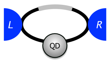
(a)

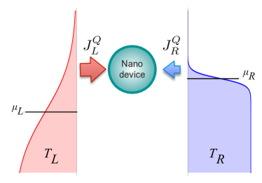
(b)

Figure 1: (a) A schematic of a quantum-dot interferometer. The hopping along the direct conducting channel between the two reservoirs (the gray region) can be adjusted. (b) The setting of electrical and thermal voltages for a heat engine: $T_{L}>T_{R}$ and $\mu_{L}<\mu_{R}$.

It is possible to manipulate quantum coherence to achieve a better performance by amplifying either positive or negative thermopower, but we need a different discipline of optimization. As a concrete illustration, we focus on a setup for a heat engine where temperature gradient drives the current flow against the bias voltage (Fig. 1b). For this case, we improve thermoelectricity by amplifying negative thermopower by tuning the bias voltage up to the stopping bias voltage.

In addition, we are particularly concerned with the situation where the temperature scale is much smaller than the resonant peak width of the dot. Although this is a typical situation for semiconductor quantum dots, it makes the system nonthermoelectric with $ZT\sim 0.1$ if it is simply coupled with the reservoirs, disconnecting the gray line in Fig. 1a (see Fig. 2a below) . We demonstrate that with a small tweaking in designing a nanostructure, one can turn such a non-thermoelectric system into being thermoelectric, i.e., by making and adjusting a direct conducting channel between the reservoirs. This thermoelectric enhancement occurs in both efficiency and output power and remains effective in the nonlinear regime.

The paper is organized as follows. We start in Sec. II by giving a phenomenological discussion of how the Fano resonance can enhance the figure of merit. Section III introduces the microscopic model of a quantum-dot interferometer in nonequilibrium. The correspondence between phenomenological parameters introduced in Sec. II and microscopic parameters is presented. In Sec. IV, we review how to obtain exactly Landauer-type formulas of nonlinear flows using the nonequilibrium Green function approach, as well as how to incorporate strong Coulomb interaction on the dot in a simple, analytical way. Sections V and VI constitute our main results: Sec. V summarizes analytical expressions of nonlinear flows of particle, energy, and heat; Sec. VI demonstrates and discusses how the efficiency and the power output get enhanced by the Fano resonance in both linear and nonlinear transport for a quantum dot with or without strong correlation. We discuss further in Sec. VII the criteria on where in the parameters we should look for better efficiency and output power. Finally we conclude in Sec. VIII. In Appendix A and B, we present one integral formula and summarize linear-response quantities for convenience.

II Phenomenology of thermoelectric enhancement

We start by making a pedagogical exposition of how transport affects and possibly enhances thermoelectric performance, especially the figure of merit $ZT$. One can gain an invaluable insight into the Fano effect by examining the linear response theory at low temperature García-Suárez et al. (2013), ignoring phonon contribution and Coulomb interaction. In that case, the scattering matrix theory can connect various transport quantities with the transmission spectrum $\mathcal{T}(\varepsilon)$ at the electrochemical potential $\mu$ (see also Appendix B). Among them, the Cutler-Mott formula Cutler and Mott (1969) gives an estimate of thermopower via the temperature-dependent conductance $G(\mu,T)$ by $S\approx-(\pi^{2}k_{B}^{2}T/{3e})d\log G(\mu,T)/d\mu$. Therefore, in the low temperature, we can directly connect the figure of merit $ZT$ with the transmission spectrum as

$$ZT\approx\frac{\pi^{2}}{3}\bigg{(}k_{B}T\frac{d\ln\mathcal{T}(\mu)}{d\mu}\bigg{)}^{2}.$$ (3)

The formula shows that to enhance $ZT$, one needs to find materials with the transmission spectrum $\mathcal{T}(\varepsilon)$ whose logarithmic slope is sufficiently large — with strongly and asymmetrically energy-dependent resonances around $\mu$.

When a single level $E_{d}$ of the dot coupling with reservoirs acquires finite resonance width $\Gamma$, the transmission spectrum usually takes a Breit-Wigner form,

$$\mathcal{T}_{\text{BW}}(\varepsilon)=\frac{\alpha\,\Gamma^{2}}{\left|\varepsilon-E_{d}+i\Gamma\right|^{2}}.$$ (4)

where $\alpha$ is the asymmetric factor [see Eq. (10)]. Then, putting it into Eq. (3), we find $ZT$ bound from above by $(\pi^{2}/3)(k_{B}T/\Gamma)^{2}$ which occurs at $\mu=E_{d}\pm\Gamma$. Since a typical resonant width $\Gamma$ in nanostructure is larger than the temperature scale, it is quite hard to achieve $ZT$ of the order of unity, except for a system with an extremely sharp peak like the Kondo resonance.

One finds the situation drastically different if $\mathcal{T}(\varepsilon)$ has a node such as $\mathcal{T}(\varepsilon)\propto(\varepsilon-\epsilon_{\text{node}})^{k}$ (for $k>0$) Bergfield and Stafford (2009); Bergfield et al. (2010). Then Eq. (3) suggests the figure of merit diverges at low temperature when the electrochemical potential crosses the node energy $\epsilon_{\text{node}}$ as $ZT\propto(k_{B}T)^{2}/(\mu-\epsilon_{\text{node}})^{2}$. Such divergence turns out to be cut off by finite temperature effect so that this leads to a universal mechanism of providing an order-of-unity $ZT$, even if $\Gamma$ is much larger than $k_{B}T$.

A great advantage of nanoscale systems is that one can make such a transmission node or nodify the spectrum $\mathcal{T}(\varepsilon)$ of any materials by manipulating how a nanostructure connects with the surroundings, i.e., by the Fano effect Finch et al. (2009); García-Suárez et al. (2013); Bevilacqua et al. (2016); Menichetti et al. (2018). One can control the effect by changing gate voltages along the direct conducting channel of a quantum-dot interferometer, or rotating the side group of a single-molecule junction. This contrasts with bulk materials whose $\mathcal{T}(\varepsilon)$ is seen as intrinsic, being always proportional to the local DOS. The transmission spectrum subject to the Fano effect is expressed by the so-called Fano formula Fano (1961) (see also Ref. Miroshnichenko et al. (2010) and references therein),

$$\mathcal{T}_{\text{Fano}}(\varepsilon)=\mathcal{T}_{0}\left|\frac{\varepsilon-E_{d}+q\Gamma}{\varepsilon-E_{d}+i\Gamma}\right|^{2},$$ (5)

where constant $\mathcal{T}_{0}$ describes the transmission of conducting channel and the Fano parameter $q$, which may be either complex or real, accounts for the asymmetry of the transmission profile. The Fano effect is an outcome of the quantum interference between the two transport channels via discrete and continuum levels. The node of $\mathcal{T}(\varepsilon)$ is located at $E_{d}-\Gamma\mathop{\mathrm{Re}}\nolimits q$, so that we expect an order-of-unity $ZT$ when we set $\mu$ around this Fano resonance dip even for $k_{B}T\lesssim\Gamma$.

Although the above phenomenological argument is quite useful to draw a rough picture of how we may expect the Fano effect to improve thermoelectric performance, we should bear in mind that the above is based on the linear response theory, not to mention on the low-temperature expansion. To gauge thermoelectric performance in nanostructures, we need to take account of two additional factors: nonlinear transport and interaction Kim and Hershfield (2003); López and Sánchez (2013); Azema et al. (2014); Sierra and Sánchez (2014); Whitney (2014). In the next section, we will work out the microscopic model of a quantum-dot interferometer and show how these phenomenological parameters constituting $\mathcal{T}_{\text{Fano}}(\varepsilon)$ can be controlled in practice.

III Microscopic model

III.1 Microscopic Hamiltonian

As a concrete microscopic realization of a system with the Fano resonance effect, we consider a quantum-dot interferometer (see Fig. 1a), a quantum dot embedded in the ring geometry and coupling with two reservoirs (the left and right reservoirs $a=L,R$) with different electrochemical potentials $\mu_{a}$ and temperatures $T_{a}$. To operate it as a heat engine, we arrange $T_{L}>T_{R}$ and $\mu_{L}<\mu_{R}$ to make the temperature voltage drive the heat flow against the potential bias (Fig. 1b). We assume a single spin-degenerate discrete level of the dot predominantly contributes to transport. With interaction on the dot, the model is essentially the single-impurity Anderson model augmented by the direct hopping between the reservoirs Hofstetter et al. (2001); Kim and Hershfield (2003). A similar model has also been studied in examining the Rashba spin-orbit interaction effect Sun et al. (2005); Crisan et al. (2009); Taniguchi and Isozaki (2012).

The total Hamiltonian is $H=H_{D}+H_{T}+H_{A}+\sum_{a=L,R}H_{a}$, where $H_{D}$ represents the dot Hamiltonian; $H_{T}$, the hopping between the dot and the leads; and $H_{A}$, the direct hopping between the left and right leads. They are given by

$$H_{D}=\sum_{\sigma}\epsilon_{d}\,\hat{n}_{\sigma}+U\hat{n}_{\uparrow}\hat{n}_{\downarrow},$$ (6)

$$H_{T}=\sum_{a=L,R}\sum_{\boldsymbol{k},\sigma}\left(V_{d\sigma a}\,d^{\dagger}_{\sigma}c_{a\boldsymbol{k}\sigma}+V_{ad\sigma}\,c^{\dagger}_{a\boldsymbol{k}\sigma}d_{\sigma}\right),$$ (7)

$$H_{A}=\sum_{\boldsymbol{k},\sigma}\left(V_{LR}\,c^{\dagger}_{L\boldsymbol{k}\sigma}c_{R\boldsymbol{k}\sigma}+V_{RL}\,c^{\dagger}_{R\boldsymbol{k}\sigma}c_{L\boldsymbol{k}\sigma}\right),$$ (8)

where $\hat{n}_{\sigma}=d^{\dagger}_{\sigma}d_{\sigma}$ is the dot electron number operator. The Hamiltonian $H_{a}$ describes noninteracting electrons on the lead $a=L,R$, which can be characterized by the DOS $\rho_{a}$ in the wide-band approximation. One may incorporate the Aharonov-Bohm effect by introducing the phase factor $\phi$ of $V_{Rd\sigma}V_{d\sigma L}V_{LR}=\big{|}V_{Rd}V_{dL}V_{LR}\big{|}\,e^{i\phi}$. We will present all of our analytical results including this effect, but we will choose $\phi=0$ for numerical presentation.

III.2 Connection with the Fano formula

To effectively regulate quantum coherence via the Fano resonance effect, we need to identify phenomenological parameters introduced in Sec. II in terms of microscopic parameters of the Hamiltonian Taniguchi and Isozaki (2012). We here summarize those connections without waiting for details that we will present in the next section.

Our convention of the relaxation rates $\gamma_{a}$ due to the leads $a=L,R$ is

$$\gamma=\gamma_{L}+\gamma_{R};\qquad\gamma_{\ell}=\pi|V_{da}|^{2}\rho_{a},$$ (9)

$$\alpha=4\gamma_{L}\gamma_{R}/\gamma^{2},$$ (10)

where $\alpha$ is the asymmetric factor regarding the dot-lead couplings. The most important parameter we utilize to control quantum coherence is the dimensionless parameter $x$, defined by

$$x=4\pi^{2}\rho_{L}\rho_{R}|V_{RL}|^{2}.$$ (11)

The parameter $x$ describes how much the direct conducting channel contribute to transport. In the absence of the electron correlation on the dot, we can exactly evaluate transmission spectra $\mathcal{T}(\varepsilon)$ (see Sec. IV.3.1 below), which confirms the Fano formula (5). This enables us to identify phenomenological parameters in Eq. (5) as

$$q=\sqrt{\frac{\alpha}{4x}}\left(e^{i\phi}-xe^{-i\phi}\right),$$ (12)

$$E_{d}=\epsilon_{d}-\Gamma\sqrt{\alpha x}\cos\phi,$$ (13)

$$\Gamma=\gamma/(1+x),$$ (14)

$$\mathcal{T}_{0}=4x/(1+x)^{2}.$$ (15)

The limit $x\to 0$ corresponds to a Breit-Wigner resonance where $E_{d}\to\epsilon_{d}$ and $\Gamma\to\gamma$. Another interesting limit is when the dot-lead couplings are extremely asymmetric. In this case, transmission $\mathcal{T}(\varepsilon)$ becomes an anti-resonance, which means the dot is side-coupled to the conducting channel.

In the presence of strong interaction on the dot, the role of the Fano parameter as characterizing the asymmetric transmission profile become obscure, because $\mathcal{T}(\varepsilon)$ gets deformed also by the interaction. Accordingly, we make a point of using Eqs. (12)–(15) as the definitions of our controlling parameters (see also the argument in Sec. IV.3).

IV Nonlinear flows of particle, energy and heat

IV.1 Current formulas

One can evaluate nonlinear flows of the particle, the energy, and the heat (denoted by $I$, $J^{E}$, and $J^{Q}$), using nonequilibrium Green functions techniques along the standard line of treatment Hofstetter et al. (2001); Kim and Hershfield (2003); Meir and Wingreen (1992); Haug and Jauho (2008). Expressions of these flows usually involve the lesser Green function of the dot as well as the retarded one. However, in the case where the dot-reservoir couplings are proportional to each other, one can safely eliminate the lesser Green function by using the conservation laws of particle and energy. Meir and Wingreen (1992). Accordingly, we can express those flows only by using the retarded Green function even if the strong interaction is present on the dot. Choosing the left reservoir as the reference, we can write those nonlinear inflows (per spin) to the dot as

$$I_{L}=\int\frac{d\varepsilon}{h}\mathcal{T}(\varepsilon)\left[f_{L}(\varepsilon)-f_{R}(\varepsilon)\right],$$ (16)

$$J_{L}^{E}=\int\frac{d\varepsilon}{2h}\mathcal{T}(\varepsilon)\varepsilon\left[f_{L}(\varepsilon)-f_{R}(\varepsilon)\right],$$ (17)

$$J_{L}^{Q}=\int\frac{d\varepsilon}{h}\mathcal{T}(\varepsilon)(\varepsilon-\mu_{L})\left[f_{L}(\varepsilon)-f_{R}(\varepsilon)\right],$$ (18)

where $h$ is the Planck constant and $f_{a}(\varepsilon)=[e^{(\varepsilon-\mu_{a})/k_{B}T_{a}}+1]^{-1}$ is the Fermi distribution on the lead $a$ with $T_{a}$ and $\mu_{a}$. They take exactly the same forms as the Landauer-Büttiker formulas by using the effective transmission function $\mathcal{T}(\varepsilon)$, which is defined in terms of the exact retarded Green function $G^{R}(\varepsilon)$. For the present case of a quantum-dot interferometer, we find $\mathcal{T}(\varepsilon)$ as Taniguchi and Isozaki (2012)

$$\mathcal{T}(\varepsilon)=\mathcal{T}_{0}-\mathop{\mathrm{Im}}\nolimits\left[\mathcal{T}_{q}\,G^{R}(\varepsilon)\Gamma\right],$$ (19)

$$\mathcal{T}_{q}=\mathcal{T}_{0}\,(q-i)(q^{*}-i).$$ (20)

We emphasize that while one usually derives the Landauer-Büttiker formula assuming the one-particle scattering theory Sivan and Imry (1986); Butcher (1990); Sánchez and López (2016); Benenti et al. (2017), the above Landauer-like description of nonlinear flows is exact, whether with or without the interaction on the dot. All the correlation effect is encoded in $\mathcal{T}(\varepsilon)$, and its validity goes beyond the one-particle approximation.

IV.2 Efficiency and output power

To assess the nonlinear thermoelectric performance as a heat engine, we mainly use two benchmarks: the output power $\mathcal{P}$ and the thermal efficiency $\eta$. Because of our configuration $\Delta\mu=\mu_{R}-\mu_{L}>0$ and $\Delta T=T_{L}-T_{R}>0$, the output power $\mathcal{P}$ and the efficiency $\eta$ are defined by

$$\mathcal{P}=\sum_{a}J_{a}^{Q}=(\mu_{R}-\mu_{L})I_{L},$$ (21)

$$\eta=\frac{\mathcal{P}}{J^{Q}_{L}}=\frac{(\mu_{R}-\mu_{L})I_{L}}{J_{L}^{Q}}.$$ (22)

The system works as a heat engine for a positive output power $\mathcal{P}>0$ with a positive heat inflow from the left reservoir $J_{L}^{Q}>0$.

Since the nonlinear flows are expressed by the Landauer-like formulas (16)–(18), its nonlinear transport is fully consistent with thermodynamics, namely, the positive entropy flow (the second law of thermodynamics). This means the efficiency $\eta$ is bound from above by the Carnot efficiency $\eta_{C}=\Delta T/T_{L}$. Moreover, quantum mechanics also bounds the power output $\mathcal{P}$ from above Whitney (2014): $\mathcal{P}$ should be smaller than $A_{0}(\pi k_{B}\Delta T)^{2}/h$ (with $A_{0}\approx 0.0321$) for the two-terminal single-level dot. Later in Sec. VI, we make a point of normalizing the output power $\mathcal{P}$ by $\mathcal{P}_{\Delta T}=k_{B}^{2}(T_{L}-T_{R})^{2}/4h$. In this unit, this quantum upper bound corresponds to $4\pi^{2}A_{0}\approx 1.267$.

IV.3 Evaluating the retarded Green function

To find nonlinear flows of a quantum-dot interferometer according to Eqs. (16)–(18), we need the dot’s retarded Green function $G^{R}(\varepsilon)$ out of equilibrium, connecting with the leads with different temperatures and electrochemical potentials. While we can obtain it exactly for a noninteracting dot, we can no longer do so if the dot involves strong interaction. For the latter case, we will make a simple yet effective analytical approximation suitable to describe charge-blocking physics that the strong correlation induces.

IV.3.1 Noninteracting dot

For a noninteracting dot, one finds exactly the retarded Green function Hofstetter et al. (2001) to be

$$G^{R}(\varepsilon)=\frac{1}{\varepsilon-E_{d}+i\Gamma}.$$ (23)

where $E_{d}$ and $\Gamma$ were given in Eqs. (13) and (14) (see also derivations by the diagram approach Kim and Hershfield (2003), the equation of motion Crisan et al. (2009) or the Kelshy path integral Taniguchi and Isozaki (2012)). Indeed, such connections were established by using the above into Eq. (19). The effective transmission $\mathcal{T}(\varepsilon)$ becomes the Fano formula,

$$\mathcal{T}(\varepsilon)=\mathcal{T}_{\text{Fano}}(\varepsilon),$$ (24)

with parameters given in Eqs.(12)–(15).

IV.3.2 Strong correlation on the dot and Coulomb blockade

It has been known that the strong correlation out of equilibrium is quite hard to treat systematically. One-particle approximations such as the Hartree-Fock theory are valid only for weak interaction, failing to explain strong correlation effects. Moreover, it is somewhat embarrassing to find that a nonequilibrium perturbation calculation regarding the interaction sometimes gives results that disrespect fundamental laws such as the current conservation Hershfield et al. (1992); Taniguchi (2014). To make a sensible assessment of the efficiency, it is crucial to abide by the conservation laws. Below, we will use a simple yet effective analytical approximation that conforms to the conservation of the particle and the energy as well as the spectral sum rule of the dot spectral function $-\pi^{-1}\mathop{\mathrm{Im}}\nolimits\int d\varepsilon\,G^{R}_{\sigma}(\varepsilon)=1$.

We focus on the strongly correlated case where the interaction $U$ is much larger than the resonant peak width or temperature. This is a typical situation of a quantum dot where charge blocking physics (the Coulomb blockade effect) dominates. Due to the strong Coulomb repulsion on the dot, the dot energy increases by the presence of another electron and depends on its occupation. Therefore, we may well view its energy as $\epsilon_{d}+U\hat{n}_{\bar{\sigma}}$ (with $\bar{\sigma}=-\sigma$). When we ignore dynamical fluctuations of the dot number operator, this leads to the following approximation of the retarded Green function Taniguchi (2017):

$$G_{\sigma}^{R}(\varepsilon)\approx\left\langle\frac{1}{\varepsilon-E_{d}-U\hat{n}_{\bar{\sigma}}+i\Gamma}\right\rangle$$ (25)

$$\quad=\frac{1-\langle\hat{n}_{\bar{\sigma}}\rangle}{\varepsilon-E_{d}+i\Gamma}+\frac{\langle\hat{n}_{\bar{\sigma}}\rangle}{\varepsilon-E_{d}-U+i\Gamma}.$$ (26)

The treatment corresponds to the Hubbard I approximation, which one can also derive within the equation-of-motion method by decoupling higher-order correlators Hubbard (1963); Hewson (1966). Unlike the treatment of Ref. Meir et al. (1991), it ignores the correlation effect on the resonant width and the Kondo correlation that become prominent at extremely low temperature (below the Kondo temperature). The approximation has been shown to capture quite well the essence of correlation effects in nonlinear responses above the Kondo temperature, and it was recently used to successfully explain strongly nonlinear thermal voltage observed in interacting quantum dots Sierra and Sánchez (2014).

To complete the approximation, we still have to determine the average occupation $\langle\hat{n}_{\bar{\sigma}}\rangle$. This is done by requiring self-consistently the particle conservation out of equilibrium, which we can solve analytically. For a quantum-dot interferometer, one can write the particle conservation as Taniguchi and Isozaki (2012); Taniguchi (2014)

$$\langle\hat{n}_{\sigma}\rangle=-\frac{1}{\pi}\int d\varepsilon\,\bar{f}(\varepsilon)\mathop{\mathrm{Im}}\nolimits G_{\sigma}^{R}(\varepsilon),$$ (27)

where $\bar{f}$ is the weighted Fermi distribution defined by

$$\bar{f}(\varepsilon)=\sum_{a=L,R}\frac{\Gamma^{\prime}_{a}}{\Gamma}f_{a}(\varepsilon),$$ (28)

$$\Gamma^{\prime}_{a}=\frac{\gamma_{a}+x\gamma_{\bar{a}}+2\sqrt{x\gamma_{a}\gamma_{\bar{a}}}\sin\phi_{a}}{(1+x)^{2}},$$ (29)

with the convention $\phi_{R}=-\phi_{L}=\phi$ and $\bar{L}=R$ etc. Since our problem is spin-independent, by putting Eq. (26), we can readily find the solution $n_{d}=\langle\hat{n}_{\uparrow}+\hat{n}_{\downarrow}\rangle$ of the self-consistent Eq. (27). (One can easily extend the treatment to the spin-dependent case as well.) We prefer organizing the solution as

$$n_{d}=\frac{2n_{0}(E_{d})}{1+n_{0}(E_{d})-n_{0}(E_{d}+U)},$$ (30)

where $n_{0}(E_{d})$ is the average occupation of a noninteracting dot per spin as a function of $E_{d}$. Using Eq. (43), we can obtain its explicit form as

$$n_{0}(E_{d})=\sum_{a}\frac{\Gamma^{\prime}_{a}}{\Gamma}\left[\frac{1}{2}-\frac{1}{\pi}\mathop{\mathrm{Im}}\nolimits\psi(\tfrac{1}{2}+z_{a})\right],$$ (31)

where $\psi(\tfrac{1}{2}+z_{a})$ is the digamma function with the argument $z_{a}=z(\beta_{a},\mu_{a}-E_{d})$ defined by

$$z(\beta,\zeta)=\frac{\beta}{2\pi i}(\zeta+i\Gamma);\quad\zeta=\mu-E_{d}.$$ (32)

Combining all the above enables us to obtain a closed analytical approximation for a quantum-dot interferometer with strong interaction.

Let us briefly discuss the immediate consequence of this approximation. Using $n_{d}$ of Eq. (30) in Eq. (19), we find that the effective transmission $\mathcal{T}(\varepsilon)$ in the Coulomb blockade regime becomes essentially a superposition of the two Fano resonances $\mathcal{T}_{\text{Fano}}$ of Eq. (5), around $E_{d}$ (with weight $1-n_{d}/2$) and $E_{d}+U$ (with weight $n_{d}/2$):

$$\mathcal{T}(\varepsilon)=\left(1-\frac{n_{d}}{2}\right)\mathcal{T}_{\text{Fano}}(\varepsilon)+\frac{n_{d}}{2}\,\mathcal{T}_{\text{Fano}}(\varepsilon-U).$$ (33)

One needs to choose phenomenological parameters according to Eqs. (9)–(12). The form indicates that the effective transmission $\mathcal{T}(\varepsilon)$ depends on temperatures and electrochemical potentials of the leads through $n_{d}$. Numerically speaking, however, the dependence of $n_{d}$ on the thermal and electrical bias, $k_{B}\Delta T$ and $\Delta\mu$, is often negligible when the system is set up for a heat engine. This is because to make it work as a heat engine, the bias $\Delta\mu$ must be of the same order of $k_{B}\Delta T$ and usually much smaller than $\Gamma$. The major role of strong interaction in a quantum-dot interferometer is to make the effective transmission split into two Fano resonances with reduced weights.

V Analytical expressions of nonlinear flows

Having obtained the effective transmission $\mathcal{T}(\varepsilon)$ for either a noninteracting or interacting dot [as in Eq. (24) or Eq. (33)], we are now in a position to write down nonlinear flows defined by Eqs. (16)–(18). We can reach their explicit forms by completing the energy integrals by using the formula (43) in Appendix A.

V.1 Noninteracting quantum dot

By applying Eq. (43) to Eqs. (16)–(18), it is straightforward to obtain analytical formulas for $I_{L}$, $J^{E}_{L}$ and $J^{Q}_{L}$. With $\zeta_{a}=\mu_{a}-E_{d}$, we organize the results as

$$I_{L}=\mathcal{I}(\beta_{L},\zeta_{L})-\mathcal{I}(\beta_{R},\zeta_{R}),$$ (34)

$$J_{L}^{E}=E_{d}I_{L}+\mathcal{J}(\beta_{L},\zeta_{L})-\mathcal{J}(\beta_{R},\zeta_{R}),$$ (35)

and heat flow is $J_{L}^{Q}=J_{L}^{E}-\mu_{L}I_{L}$. Functions $\mathcal{I}(\beta,\mu)$ and $\mathcal{J}(\beta,\mu)$ describe contributions from each leads, and involve Euler’s digamma function:

$$h\,\mathcal{I}(\beta,\zeta)=\mathcal{T}_{0}\zeta-\Gamma\mathop{\mathrm{Im}}\nolimits\left[\mathcal{T}_{q}\left(\psi(\tfrac{1}{2}+z)-\log\beta\Gamma\right)\right],$$ (36)

$$h\,\mathcal{J}(\beta,\zeta)=\mathcal{T}_{0}\Big{(}\frac{\zeta^{2}}{2}+\frac{\pi^{2}}{6\beta^{2}}\Big{)}-\Gamma\mathop{\mathrm{Im}}\nolimits\Big{[}\mathcal{T}_{q}\zeta$$

$$\qquad\qquad\qquad-i\Gamma\mathcal{T}_{q}\left\{\psi(\tfrac{1}{2}+z)-\log\beta\Gamma\right\}\Big{]},$$ (37)

with $z=z(\beta,\zeta)$ in Eq. (32). When one disconnect the direct hopping between the reservoirs ($x\to 0$), they reduce (with $E_{d}\to\epsilon_{d}$ and $\Gamma\to\gamma$) to

$$h\,\mathcal{I}(\beta,\zeta)=-\alpha\Gamma\mathop{\mathrm{Im}}\nolimits\left[\psi(\tfrac{1}{2}+z)\right],$$ (38)

$$h\,\mathcal{J}(\beta,\zeta)=\alpha\Gamma^{2}\left[\mathop{\mathrm{Re}}\nolimits\psi(\tfrac{1}{2}+z)-\ln\beta\gamma\right].$$ (39)

V.2 Quantum dot with interaction

In the presence of strong correlation on the dot, Eq. (33) tells us that the effective transmission $\mathcal{T}(\varepsilon)$ becomes a superposition of the two Fano resonances, around $E_{d}$ and $E_{d}+U$. Hence nonlinear flows are also expressed by a superposition of these two contributions.

$$I_{L}=\left(1-\frac{n_{d}}{2}\right)\left[\mathcal{I}(\beta_{L},\zeta_{L})-\mathcal{I}(\beta_{R},\zeta_{R})\right]$$

$$\qquad\quad+\frac{n_{d}}{2}\left[\mathcal{I}(\beta_{L},\zeta_{L}-U)-\mathcal{I}(\beta_{R},\zeta_{R}-U)\right],$$ (40)

$$J_{L}^{E}=E_{d}I_{L}+\left(1-\frac{n_{d}}{2}\right)\left[\mathcal{J}(\beta_{L},\zeta_{L})-\mathcal{J}(\beta_{R},\zeta_{R})\right]$$

$$\qquad\quad+\frac{n_{d}}{2}\left[\mathcal{J}(\beta_{L},\zeta_{L}-U)-\mathcal{J}(\beta_{R},\zeta_{R}-U)\right].$$ (41)

Using these $I_{L}$ and $J_{L}^{E}$, the heat current becomes $J_{L}^{Q}=J_{L}^{E}-\mu_{L}I_{L}$.

VI Numerical results and discussion

In this section, we present numerical results to support how one can greatly improve nonlinear thermoelectric performance by regulating quantum coherence via the Fano resonance effect. Based on the analytical results in Sec. III, we now make a fully nonlinear analysis, focusing on the thermal efficiency and the output power as benchmarks. For a better heat engine, we will intend to amplify a negative thermopower, which makes us choose $q>0$ and $\phi=0$ [see Eq. (12)]. If we aim to enhance a positive thermopower, we have to choose $q<0$ instead.

We choose to fix the temperature and electrochemical potential of the left reservoir as a reference while changing those of the right reservoir, assuming the symmetric dot-reservoir couplings $\alpha=1$. In addition, for most calculations, we take the temperature much smaller than the resonant width (setting $k_{B}T_{L}=0.2\gamma$). Such a situation common in nanostructures is certainly unfavorable to achieve high thermoelectricity ($ZT\sim 0.1$ without the Fano effect as in Fig. 2a below). Nevertheless, we will demonstrate that we can improve the thermoelectric performance 10 times as much, by adjusting the Fano resonance effect.

We deliberately present all the results in a way that one can easily compare between linear and nonlinear responses. For convenience, we summarize the explicit forms of linear-response quantities as well as the Onsager coefficients in Appendix B.

VI.1 Noninteracting quantum dot

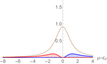
(a)

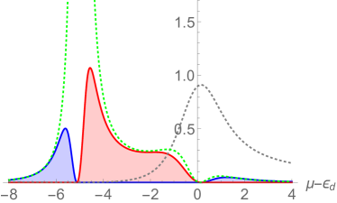
(b)

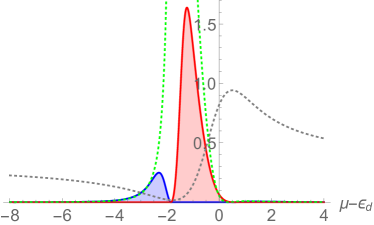
(c)

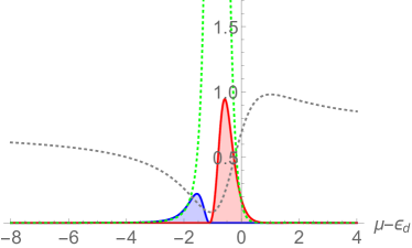
(d)

Figure 2: The figure of merit $ZT$ at $k_{B}T=0.2\gamma$, as a function of $\mu-\epsilon_{d}$ by changing (a) $x=0$ ($q=\infty$), (b) $x=0.01$ ($q=4.95$), (c) $x=0.1$ ($q=1.42$) and (d) $x=0.3$ ($q=0.64$). Red and blue indicate corresponding thermopower is positive or negative. Green lines show $ZT$ at the zero-temperature limit. Dotted lines correspond to the normalized conductance.

VI.1.1 Linear responses

We start by examining linear-response quantities, focusing the figure of merit $ZT$ of Eq. (51). Figure 2 shows the figure of merit $ZT$ at $k_{B}T=0.2\gamma$ as a function of $\mu-\epsilon_{d}$ by changing the parameter $x$ (or the Fano parameter $q$). Red (blue) shade corresponds to a negative (positive) thermopower region. The zero-temperature limit of $ZT$ (green lines) as well as the normalized conductance (dotted lines) is also shown in the same figure. Because $k_{B}T$ is much smaller than the peak width $\gamma$, $ZT$ is small ($\approx 0.11$) at $x=0$, but it quickly reaches more than unity by introducing a small amount of $x$ ($ZT=1.07$ for $x=0.01$, $1.64$ for $x=0.1$, and $0.94$ for $x=0.3$). Figures 3a and 3b show the density plot of $ZT$ as a function of $\mu-E_{d}$ and $x$. We see, if we choose a larger value of $k_{B}T$, $ZT$ can get even larger. We find the value of $ZT$ exceeds 5 at $k_{B}T=\gamma$ (not shown), though such a situation may be hard to realize in nanostructure systems except for extremely low-temperature Kondo regime. As argued in Sec. II, we anticipate such enhancement around the Fano resonant node $\mu-E_{d}\approx-q\Gamma$, which we depict by the green dashed lines in Fig. 3. The optimal $x$ that achieves the largest $ZT$ (hence the efficiency) is around $x=0.1$ for $k_{B}T=0.2\gamma$, and around $x=0.01$ for $k_{B}T=\gamma$. The optimal value of $x$ depends on $k_{B}T/\gamma$ and decreases with increasing $k_{B}T/\gamma$.

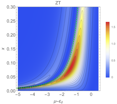
(a)

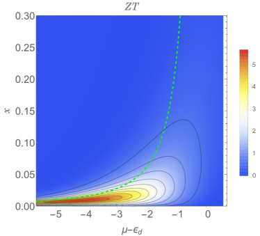
(b)

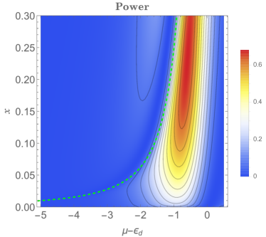
(c)

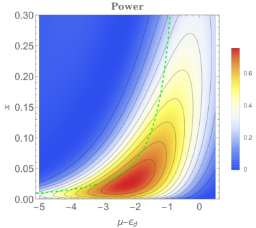
(d)

Figure 3: Density plots of the figure of merit $ZT$ and the linear-response estimate of the maximal power $\mathcal{P}_{\max}$, as a function of $\mu-\epsilon_{d}$ and $x$. (a) $ZT$ at $k_{B}T=0.2\gamma$, (b) $ZT$ at $k_{B}T=\gamma$, (c) $\mathcal{P}_{\max}$ at $k_{B}T=0.2\gamma$, (d) $\mathcal{P}_{\max}$ at $k_{B}T=\gamma$. Green dashed lines specify the location of the Fano node.

Figures 3c and 3d show the density plot of the linear-response estimate of the maximal output power $\mathcal{P}_{\max}$ in the unit of $\mathcal{P}_{\Delta T}=(k_{B}\Delta T)^{2}/4h$. The quantity is nothing but $hGS^{2}/k_{B}^{2}=\mathcal{K}_{1}^{2}/\mathcal{K}_{0}$, discussed in Appendix B [see Eq. (54)]. We find the maximal achievable power $\mathcal{P}_{\max}$ is less sensitive to the value of $k_{B}T/\gamma$. Comparing Figs. 3a and 3c, or 3b and 3d, we see that the optimal sets of parameters $(x,\epsilon_{d}-\mu)$ to maximize $(ZT)$ or $\mathcal{P}_{\max}$ differs, but they are not so far apart when $x$ is finite. We can recapitulate the linear-response performance by drawing the power-efficiency diagram in Fig. 4. We see that introducing $x$ helps drastically enhance it in both cases $k_{B}T=0.2\gamma$ and $k_{B}T=\gamma$.

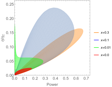
(a)

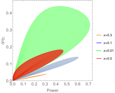
(b)

Figure 4: Linear-response estimate of the power-efficiency diagram at (a) $k_{B}T=0.2\gamma$ and (b) $k_{B}T=\gamma$, by changing $x$: $x=0.0$ (red), $x=0.01$ (green), $x=0.1$ (blue) and $x=0.3$ (orange).

VI.1.2 Nonlinear responses

We now examine how nonlinear thermoelectric performance can be possibly improved by utilizing the Fano effect or the parameter $x$. The analysis of linear-response quantities tells us what parameter range we should look at to improve it. Seeing Figs. 3a and 3c, we choose to examine mainly the setting $k_{B}T_{L}=2k_{B}T_{R}=0.2\gamma$ with $x=0.01$ and $x=0.1$, where the corresponding Carnot efficiency is $\eta_{C}=0.5$.

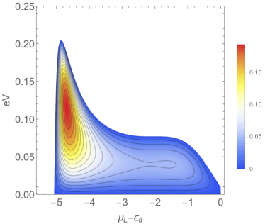
(a) $\eta/\eta_{C}$ at $x=0.01$.

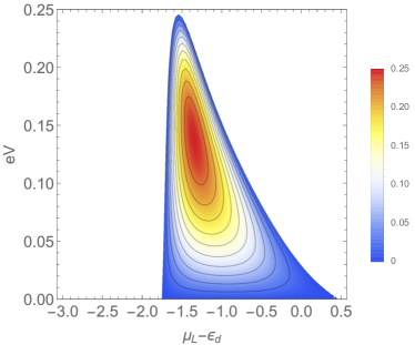
(b) $\eta/\eta_{C}$ at $x=0.1$.

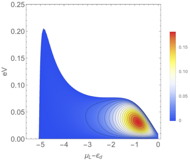
(c) $\mathcal{P}$ at $x=0.01$.

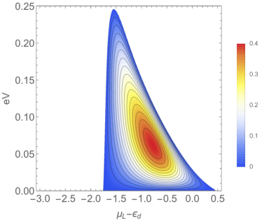
(d) $\mathcal{P}$ at $x=0.1$.

Figure 5: Evolution of nonlinear efficiencies $\eta/\eta_{C}$ and the output powers $\mathcal{P}$ by changing gate and bias voltages. The setting is $k_{B}T_{L}=2k_{B}T_{R}=0.2\gamma$ (with $\eta_{C}=0.5$). We normalize $\mathcal{P}$ by $\mathcal{P}_{\Delta T}$.

Figures 5 show density plots of nonlinear efficiencies $\eta$ (modulo $\eta_{C}$) and output powers $\mathcal{P}$ (modulo $\mathcal{P}_{\Delta T}$) for $x=0.01$ (a, c) and $x=0.1$ (b,d). We find the maximal values of the efficiencies reaches $0.20\eta_{C}$ (for $x=0.01$) or $0.25\eta_{C}$ (for $x=0.1$), exceeding their linear-response estimates. For the case of $x=0.01$, one sees that the settings of gate and bias voltages for maximizing either the efficiency or the output power are irreconcilable. For instance, at the gate voltage achieving the highest efficiency, its output power almost vanishes, as was argued in Ref. Nakpathomkun et al. (2010). For the case of $x=0.1$, however, the two conditions are more compatible, and both a higher $\eta$ and a larger $\mathcal{P}$ are achieved in comparing with $x=0.01$. The power-efficiency diagrams in Fig. 6 clearly show this difference in their behaviors. We see that for the case of $x=0.1$, the efficiency and the output power are well balanced for a finite range of the gate voltage $\mu_{L}$.

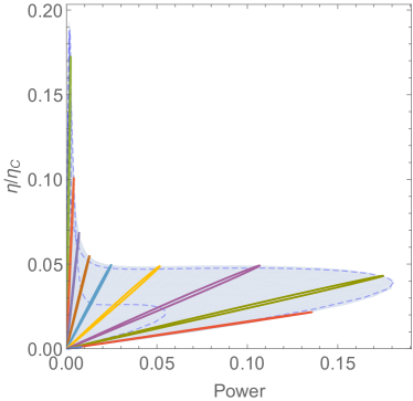
(a) $x=0.01$

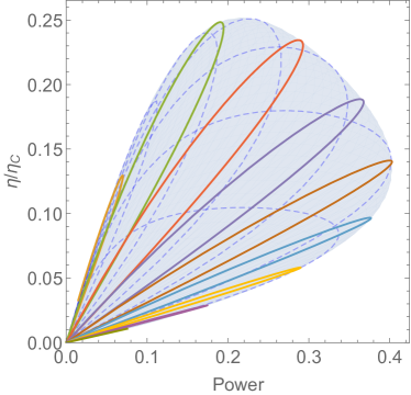
(b) $x=0.1$

Figure 6: Power-efficiency diagrams of Fig. 5. Color lines correspond to the evolution by changing bias voltage with a fixed gate voltage, and dashed lines correspond to the one by changing the gate voltage with a fixed bias voltage.

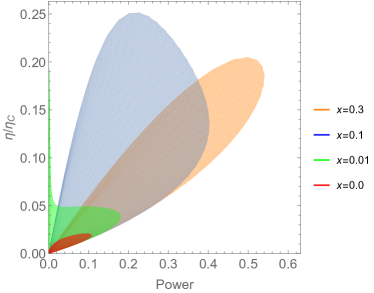
(a) $T_{R}=0.5T_{L}$ ($\eta_{C}=0.50$)

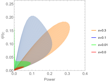
(b) $T_{R}=0.05T_{L}$ ($\eta_{C}=0.95$)

Figure 7: Comparison of the power-efficiency diagrams at different $k_{B}T_{R}$. Other parameters are the same with Figs. 5 and 6. The power output is normalized by $\mathcal{P}_{\Delta T}$ for both cases.

To attain even higher efficiency and output power, one may place a system subject to a larger temperature difference, because the linear-response theory predicts the efficiency proportional to $\eta_{C}$ and the power output, to $\eta_{C}^{2}$, though nonlinear effects may well suppress such behavior. We expect, however, the present thermoelectric enhancement is likely to survive for a large temperature difference because it is a universal mechanism due to the Fano resonance effect (see Sec. II). Figures 7a and 7b compare the power-efficiency diagrams between the two settings: (a) $k_{B}T_{L}=2k_{B}T_{R}=0.2\gamma$ (with $\eta_{C}=0.5$), and (b) $k_{B}T_{L}=20k_{B}T_{R}=0.2\gamma$ (with $\eta_{C}=0.95$). By normalizing the efficiency $\eta$ by $\eta_{C}$, and the output power $\mathcal{P}$ by $\mathcal{P}_{\Delta T}$, we can directly compare those diagrams with Fig. 4a. We first notice that the linear-response estimate reasonably captures the overall tendency for each $x$ in this fully nonlinear regime. There is a noticeable saturation in the highest efficiency and a severe reduction of the output power, though. We can attribute those to nonlinear thermal effects, which we will discuss further in Sec. VII. Comparing with the thermoelectric performance at $x=0$, the enhancement effect due to finite $x$ is significant. For the case of $\eta_{C}=0.5$, the power-efficiency improves from $(\mathcal{P}_{\max},\eta_{\max})=(0.11\mathcal{P}_{\Delta T},0.02\eta_{C})$ at $x=0$ to $(0.40\mathcal{P}_{\Delta T},0.25\eta_{C})$ at $x=0.1$, or $(0.54\mathcal{P}_{\Delta T},0.20\eta_{C})$ at $x=0.3$; for the case of $\eta_{C}=0.95$, from $(\mathcal{P}_{\max},\eta_{\max})=(0.06\mathcal{P}_{\Delta T},0.015\eta_{C})$ at $x=0$ to $(0.21\mathcal{P}_{\Delta T},0.20\eta_{C})$ at $x=0.1$, or $(0.31\mathcal{P}_{\Delta T},0.18\eta_{C})$ at $x=0.3$. The efficiency improves more than 10 times, while the output power gets amplified nearly 5 times.

VI.2 Quantum dot with interaction

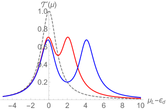
(a) $x=0$

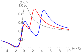
(b) $x=0.1$

Figure 8: Effective transmission $\mathcal{T}(\mu)$ for an interacting dot as a function of $\mu-\epsilon_{d}$ by changing $U$: $U/\gamma=0$ (dashed gray lines), $2$ (red lines), and $4$ (blue line). The results are shown for (a) $x=0$ and (b) $x=0.1$.

As argued in Sec. IV.3.2, we incorporate the strong interaction on the dot in the effective transmission by Eq. (33). Figure 8 illustrates how $\mathcal{T}(\varepsilon)$ describes the Coulomb blockade peaks around $\mu-\epsilon_{d}=E_{d}$ and $E_{d}+U$ (Fig. 8a), and its deformations by the Fano resonances (Fig. 8b). Since nonlinear flows become a superposition of two Fano-type contributions, as in Eqs. (40) and (41), we can still apply much of the previous argument given for a noninteracting dot to an interacting dot. That means we expect enhanced thermoelectricity by the Fano resonance in an interacting dot as well.

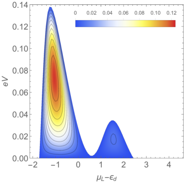
(a) $\eta/\eta_{C}$ at $U=2\gamma$

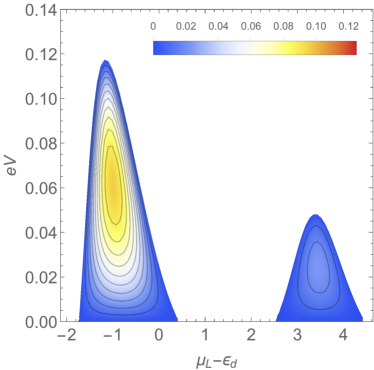
(b) $\eta/\eta_{C}$ at $U=4\gamma$

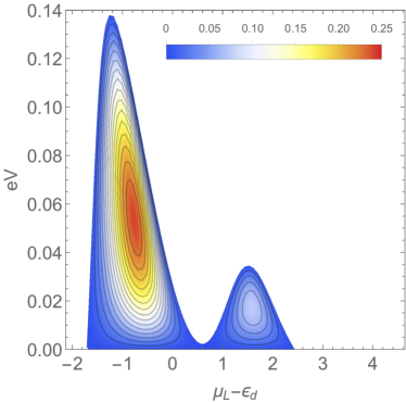
(c) $\mathcal{P}$ at $U=2\gamma$

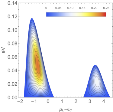
(d) $\mathcal{P}$ at $U=2\gamma$

Figure 9: The evolution of the efficiency $\eta/\eta_{C}$ and the power output $\mathcal{P}$ at $x=0.1$ by changing $U$ at $k_{B}T_{L}=2k_{B}T_{R}=0.2\gamma$ with $\eta_{C}=0.5$. The power $\mathcal{P}$ is normalized by $\mathcal{P}_{\Delta T}$.

Figures 9 show the density plots of the efficiency and the output power as a function of gate and bias voltages by changing $U/\gamma=2,4$. For a better comparison, we use the same color scheme for different values of $U$. As one sees in Fig. 9, the Fano resonance dominantly affects only one of the two Coulomb blockade peaks to enhance both the efficiency and the output power there (see also Fig. 10). Simultaneously, we notice that the highest efficiency decreases with increasing $U$, suggesting strong interaction is rather detrimental to efficiency. The power-efficiency diagrams (Fig. 10) clarify this point. For a fixed $U$, we see both the efficiency and the output power greatly enhanced by introducing finite $x$, as in a noninteracting dot. With $U=2\gamma$, we have $(\mathcal{P}_{\max},\eta_{\max})=(0.08\mathcal{P}_{\Delta T},0.02\eta_{C})$ to $(0.24\mathcal{P}_{\Delta T},0.12\eta_{C})$ at $x=0.1$ (Fig. 10a). However, the efficiency at $x=0.1$, which is most enhanced, gets suppressed by increasing $U$. One may understand it from the form of the effective transmission (33). Since the transmission peak is split into two and and the average occupation around the Fano resonance gets smaller by increasing $U$, the Fano enhancement plays a less prominent role with a larger $U$. Such interaction-induced suppression is also seen in the output power but its reduction is much more gradual.

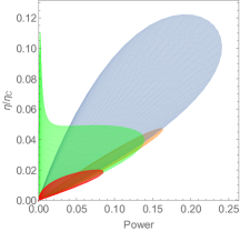
(a) $U=2\gamma$

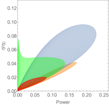
(b) $U=4\gamma$

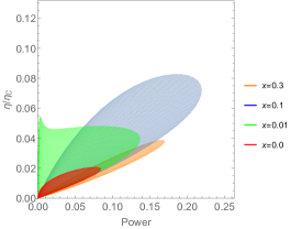
(c) $U=8\gamma$

Figure 10: Power-efficiency diagram by changing $U/\gamma=2$, $4$, $8$. Other parameters are the same as in Fig. 9. Shaded regions correspond to the evolution for $x=0$ (red), $x=0.01$ (green), $x=0.1$ (blue), and $x=0.3$ (orange).

VII Assessing nonlinear thermoelectricity

In taking advantage of quantum control to achieve better thermoelectricity, it is important to find an optimal set of relevant parameters. With a fixed $x$, we find it crucial to adjust the gate voltage for attaining a full enhancement due to the Fano effect. To assess its performance in the nonlinear transport regime, we would be better off with a quantity that can characterize nonlinear thermoelectric performance without delving into a detailed analysis of nonlinear flows. The figure of merit $ZT$ loses its authenticity beyond the linear transport Meair and Jacquod (2013); Azema et al. (2014). We here address this issue with some speculations, based on our results.

To be concrete, we take the results of a noninteracting dot with $x=0.01$ and $0.1$ (Fig. 5), where we evaluated nonlinear flows exactly. Figure 11 shows the corresponding bias voltage characteristic of the particle and heat flows at $x=0.1$. One finds that the particle flow depends almost linearly while the heat flow, highly nonlinearly. We intend to exploit the former characteristic of the particle flow in asses nonlinear thermoelectricity.

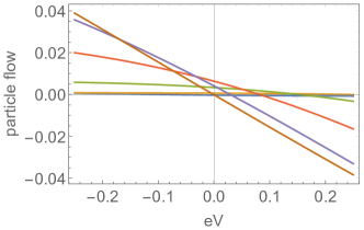
(a) Particle flow $I_{L}$

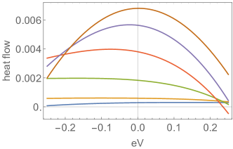
(b) Heat flow $J_{L}^{Q}$

Figure 11: Nonlinear flows of the particle and the heat at $x=0.1$ as a function of bias voltage. Parameters are the same as in Fig. 5. Different colored lines correspond to different values of the gate voltage from $\mu_{L}-\varepsilon_{d}=-2.0\gamma$ to $+0.5\gamma$.

VII.1 Output power

Since the particle flow is almost linear regarding the bias voltage, we can use much of the linear response theory to investigate the output power $\mathcal{P}$. For instance, we immediately see that $\mathcal{P}$ takes its maximum regarding the bias voltage around half the stopping potential, $\Delta\mu\equiv\mu_{R}-\mu_{L}=\Delta\mu_{\text{stop}}/2$ as in the linear response theory. What is more important in applications is the location of the optimal gate voltage to maximize the power. With other parameters fixed, we can roughly estimate it by the low-temperature expansion: $\mathcal{P}\propto[\mathcal{T}^{\prime}(\bar{\mu})]^{2}/\mathcal{T}(\bar{\mu})$ (with $\mu_{L}<\bar{\mu}<\mu_{R}$). For a real $q$, we can find an analytical solution to maximize $\mathcal{P}$ at

$$\bar{\mu}=E_{d}-\tilde{q}\,\Gamma;\quad\tilde{q}=\tfrac{\sqrt{9+8q^{2}}-3}{4q}.$$ (42)

By choosing $\bar{\mu}=\mu_{L}$, this provides an estimate of the optimal gate voltage $\mu_{L}-\epsilon_{d}\approx-0.66\gamma$ in Fig. 5c, or $\mu_{L}-\epsilon_{d}\approx-0.61\gamma$ in Fig. 5d. We see that these estimates give a reasonable agreement in both cases.

VII.2 Nonlinear efficiency

We now consider how we find the optimal gate voltage to achieve the highest nonlinear efficiency. As was discussed in Sec. II, we expect the enhancement for the efficiency to occur near the Fano node $E_{d}-\Gamma\mathop{\mathrm{Re}}\nolimits q$ (the green dashed line in Fig. 3), which gives $-5.0\gamma$ for $x=0.01$ (Fig. 5a), or $\mu-\epsilon_{d}\approx-1.58\gamma$ for $x=0.1$ (Fig. 5b). Since one can deduce the value of $q$ from the observed transmission profile, this helps us locate the optimal gate voltage.

We can make a more quantitative argument and speculate about how it connects with a linear response quantity by using the almost linear characteristic of $I_{L}$. As one notices immediately in Figs. 5a and 5b, the gate voltage optimal for efficiency almost coincides with what maximize the boundary line. The latter boundary line defines the stopping potential $\Delta\mu_{\text{stop}}$ when the particle flow vanishes. This implies that the (dimensionless) nonlinear thermopower $\Delta\mu_{\text{stop}}/k\Delta T$ may well characterize the nonlinear efficiency. Furthermore, as was demonstrated numerically for the single-impurity Anderson model Azema et al. (2014), one can somehow predict nonlinear thermopower well by using the linear-response estimate at the “operating temperature” $T_{\text{op}}=(T_{L}+T_{R})/2$. Therefore, we may conjecture that we can use the linear-response estimate of the thermopower at $T_{\text{op}}$ to assess the nonlinear efficiency. Figure 12a supports this speculation: the linear-response estimate of $\Delta\mu_{\text{stop}}$ at $T_{\text{op}}$ (red line) is compared with the nonlinear efficiency of Fig. 5b. We see that the maximum of the red line detects well the location of the gate voltage optimal for efficiency.

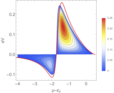
(a) $\gamma_{L}=\gamma_{R}=0.5\gamma$

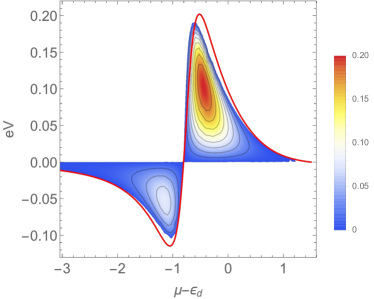
(b) $\gamma_{L}=0.05\gamma$, $\gamma_{R}=0.95\gamma$

Figure 12: Comparison of the linear thermopower at $T_{\text{op}}$ with (a) nonlinear efficiency of Fig. 5b, and (b) the case where the dot-reservoir couplings are highly asymmetric.

One way to understand this unexpected role of $T_{\text{op}}$ is due to a low-temperature expansion of $I_{L}$. The lowest-order of the temperature correction takes a form of $(\pi^{2}\mathcal{T}^{\prime}(\bar{\mu})k_{B}^{2}/6)(T_{L}^{2}-T_{R}^{2})\propto T_{\text{op}}\Delta T$ (with $\mu_{L}\leq\bar{\mu}\leq\mu_{R}$). The argument suggests that the using $T_{\text{op}}$ may not be limited for the symmetric dot-bath couplings case considered in Ref. Azema et al. (2014). In Fig. 12b, we support the view by taking a look at a dot with highly asymmetric couplings, $\gamma_{L}=0.05\gamma$ and $\gamma_{R}=0.95\gamma$ with $\alpha=0.19$. In spite of high asymmetry, we see the linear-response estimate at $T_{\text{op}}$ can tell reasonably well the location of the gate voltage optimal for nonlinear efficiency.

VII.3 Power-efficiency diagram

Figure 13 illustrates how using the operating temperature $T_{\text{op}}=T_{L}(1-\eta_{C}/2)$ helps improve a linear-response estimate of the power-efficiency diagram for the parameters chosen in Fig. 7: (a) $k_{B}T_{L}=2k_{B}T_{R}=0.2\gamma$ (with $\eta_{C}=0.5$) and $k_{B}T_{L}=20k_{B}T_{R}=0.2\gamma$ (with $\eta_{C}=0.95$). Comparing with Fig. 4a (with $\eta_{C}=0$), we see the linear-response estimate with using $T_{\text{op}}$ (Fig. 13) much improved in predicting the behavior of Fig. 7, especially regarding the output power. We find this way of the linear-response estimate of nonlinear thermoelectricity useful for finding an optimal setting of nonlinear thermoelectric performance, even in the fully nonlinear regime $\eta_{C}=0.95$.

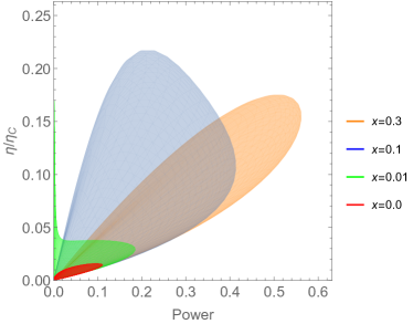
(a) $\eta_{C}=0.50$

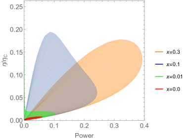
(b) $\eta_{C}=0.95$

Figure 13: Linear-response estimate of the power-efficiency diagram using $T_{\text{op}}$, for (a) $\eta_{C}=0.50$ and (b) $\eta_{C}=0.95$. Parameters are chosen to correspond with Fig. 7.

VIII Summary

We have developed a theory for enhancing the thermoelectric performance (efficiency and power) when a nanostructure acts as a heat engine. We have demonstrated that even if the temperature is much smaller than the resonant width, which is unfavorable for good thermoelectricity, one can still achieve a reasonably good thermoelectric performance by regulating quantum coherence via the Fano effect. Such thermoelectric enhancement stays effective in fully nonlinear regimes. We have shown that such thermoelectric enhancement is viable in fully nonlinear responses. With appropriate parameters, the efficiency improves up to 10 times and the power, nearly 5 times (Figs. 7 and 10). We have also estimated the optimal gate voltage that maximizes nonlinear efficiency or power. Furthermore, we argued the significance of the linear thermopower at $T_{\text{op}}$ along assessing nonlinear efficiency (Fig. 13). We believe quantum control by the Fano effect is a promising, universal approach that helps thermoelectric materials exhibit an even better thermoelectric performance, as well as turn mediocre materials into thermoelectric.

Appendix A Integral formula

We use the following integral formula to evaluate the energy integrals that appear in nonlinear flows:

$$\int^{\infty}_{-\infty}\frac{d\varepsilon}{(\varepsilon-E_{d}+i\Gamma)[e^{\beta(\varepsilon-\mu)}+1]}$$

$$\quad=\int^{\mu}_{-\infty}\frac{d\varepsilon}{\varepsilon-E_{d}+i\Gamma}+\psi(\tfrac{1}{2}+z)-\log z,$$ (43)

where $\psi(\tfrac{1}{2}+z)$ is Euler’s digamma function and the parameter $z$ is defined in Eq. (32). One can derive Eq. (43) in various ways, e.g., by summing up the Sommerfeld expansion up to infinite order (see also Ref. Taniguchi, 2018 Appendix D). The first term on the right-hand side corresponds to the zero-temperature contribution. It diverges logarithmically but will be canceled out in evaluating flows.

Appendix B Linear response quantities

In this appendix, we collect the results of the linear-response theory and connect them with the Onsager coefficients. They can be obtained by expanding our nonlinear results regarding small bias and thermal gradient. Let us introduce the dimensionless Onsager coefficients $\mathcal{K}_{n}$ (for $n=0,1,2$), which are defined by

$$\mathcal{K}_{n}=\beta^{n}\int d\varepsilon\,\mathcal{T}(\varepsilon)(\varepsilon-\mu)^{n}\,[-f^{\prime}(\varepsilon)].$$ (44)

Within the linear response theory, one can express flows of particle and heat as

$$h\begin{pmatrix}I_{L}\\ \beta J^{Q}_{L}\end{pmatrix}=\begin{pmatrix}\mathcal{K}_{0}&\mathcal{K}_{1}\\ \mathcal{K}_{1}&\mathcal{K}_{2}\end{pmatrix}\begin{pmatrix}\mu_{LR}\\ k_{B}T_{LR}\end{pmatrix},$$ (45)

if $\mu_{LR}=\mu_{L}-\mu_{R}$ and $T_{LR}=T_{L}-T_{R}$ are small. We can readily evaluate $\mathcal{K}_{n}$ as

$$\mathcal{K}_{0}=\mathcal{T}_{0}+\frac{\beta\Gamma}{2\pi}\mathop{\mathrm{Re}}\nolimits\left[\mathcal{T}_{q}\,\psi^{\prime}(\tfrac{1}{2}+z)\right],$$ (46)

$$\mathcal{K}_{1}=-\beta\Gamma\mathop{\mathrm{Im}}\nolimits\left[\mathcal{T}_{q}\left(1-z\psi^{\prime}(\tfrac{1}{2}+z)\right)\right],$$ (47)

$$\mathcal{K}_{2}=\frac{\pi^{2}}{3}\mathcal{T}_{0}+2\pi\beta\Gamma\mathop{\mathrm{Re}}\nolimits\left[\mathcal{T}_{q}\left(z-z^{2}\psi^{\prime}(\tfrac{1}{2}+z)\right)\right].$$ (48)

We note that we straightforwardly restore the results of the Sommerfeld expansion by seeing $\mathcal{K}_{0}\approx\mathcal{T}(\mu)$, $\mathcal{K}_{1}\approx\frac{\pi^{2}}{3}(k_{B}T)\mathcal{T}^{\prime}(\mu)$ and $\mathcal{K}_{2}\approx\frac{\pi^{2}}{3}\mathcal{T}(\mu)$ at low temperatures.

In terms of these dimensionless Onsager coefficients $\mathcal{K}_{n}$, standard linear-response quantities are given by

$$G=\frac{e^{2}}{2\pi\hbar}\mathcal{K}_{0}; K=\frac{k_{B}^{2}T}{2\pi\hbar}\left(\mathcal{K}_{2}-\frac{\mathcal{K}_{1}^{2}}{\mathcal{K}_{0}}\right),$$ (49)

$$S=-\frac{k_{B}}{e}\frac{\mathcal{K}_{1}}{\mathcal{K}_{0}}; \Pi=-\frac{k_{B}T}{e}\frac{\mathcal{K}_{1}}{\mathcal{K}_{0}}.$$ (50)

Therefore the figure of merit $ZT$ becomes

$$ZT=\frac{GT}{K}S^{2}=\frac{\mathcal{K}_{1}^{2}}{\mathcal{K}_{0}\mathcal{K}_{2}-\mathcal{K}_{1}^{2}}.$$ (51)

When one uses the above linear response theory with choosing $\Delta\mu=\mu_{RL}>0$ and $\Delta T=T_{LR}>0$, one finds the stopping bias potential (or the open circuit potential) that makes the particle flow vanish is given by

$$\Delta\mu_{\text{stop}}=-e\,S\Delta T=\frac{\mathcal{K}_{1}}{\mathcal{K}_{0}}k_{B}\Delta T$$ (52)

According to Eq. (21), the output power $\mathcal{P}$ becomes

$$\mathcal{P}=I\Delta\mu=\left(-\mathcal{K}_{0}\Delta\mu+\mathcal{K}_{1}k_{B}\Delta T\right)\cdot\frac{\Delta\mu}{h},$$ (53)

which we can maximize at $\Delta\mu=\Delta\mu_{\text{stop}}/2$ as

$$\mathcal{P}_{\max}=\frac{GS^{2}}{4}(\Delta T)^{2}=\frac{(k_{B}\Delta T)^{2}}{4h}\cdot\frac{\mathcal{K}_{1}^{2}}{\mathcal{K}_{0}}.$$ (54)

By introducing $v=\Delta\mu/\Delta\mu_{\text{stop}}$, one can simply write the ratio as $\mathcal{P}/\mathcal{P}_{\max}=4v(1-v)$.

The linear-response efficiency $\eta_{L}$ is also defined by Eq. (22). After some manipulation, we can write it as

$$\frac{\eta_{L}}{\eta_{C}}=\frac{v(1-v)}{1+(ZT)^{-1}-v}.$$ (55)

Accordingly, the efficiency at the maximal power ($v=1/2$) is equal to

$$\eta_{L}(\mathcal{P}_{\max})=\frac{\eta_{C}}{2}\cdot\frac{ZT}{ZT+2}.$$ (56)

We can maximize $\eta_{L}$ by changing $0<v<1$. The maximal value $\eta_{L}^{\max}$ is given by Eq. (2), when one chooses $v=(1+\eta_{L}^{\max}/\eta_{C})/2$.

References

- Rowe (2006) D. M. Rowe, ed., Thermoelectrics Handbook, Macro to Nano (Taylor & Francis, Boca Raton, 2006).
- Dubi and Di Ventra (2011) Y. Dubi and M. Di Ventra, Rev. Mod. Phys. 83, 131 (2011).
- Wang and Wang (2014) X. Wang and Z. M. Wang, eds., Nanoscale Thermoelectrics, Lecture Notes in Nanoscale Science and Technology, Vol. 16 (Springer, Cham, 2014).
- Zlatić and Monnier (2014) V. Zlatić and R. Monnier, Modern Theory of Thermoelectricity (Oxford University Press, Oxford, 2014).
- Goldsmid (2016) H. J. Goldsmid, Introduction to Thermoelectricity, Springer Series in Materials Science, Vol. 121 (Springer, Berlin, 2016).
- Majumdar (2004) A. Majumdar, Science 303, 777 (2004).
- Vining (2009) C. B. Vining, Nature Materials 8, 83 (2009).
- He and Tritt (2017) J. He and T. M. Tritt, Science 357, eaak9997 (2017).
- Dresselhaus et al. (2007) M. S. Dresselhaus, G. Chen, M. Y. Tang, R. G. Yang, H. Lee, D. Z. Wang, Z. F. Ren, J. P. Fleurial, and P. Gogna, Advanced Materials 19, 1043 (2007).
- Humphrey et al. (2002) T. E. Humphrey, R. Newbury, R. P. Taylor, and H. Linke, Phys. Rev. Lett. 89, 116801 (2002).
- Zhou et al. (2015) J. Zhou, Y. Yang, and C.-y. Zhang, Chemical Reviews 115, 11669 (2015).
- Hicks and Dresselhaus (1993a) L. D. Hicks and M. S. Dresselhaus, Phys. Rev. B 47, 12727 (1993a).
- Hicks and Dresselhaus (1993b) L. D. Hicks and M. S. Dresselhaus, Phys. Rev. B 47, 16631 (1993b).
- Mahan and Sofo (1996) G. D. Mahan and J. O. Sofo, Proceedings of the National Academy of Sciences 93, 7436 (1996).
- Finch et al. (2009) C. M. Finch, V. M. García-Suárez, and C. J. Lambert, Phys. Rev. B 79, 033405 (2009).
- Gómez-Silva et al. (2012) G. Gómez-Silva, O. Ávalos Ovando, M. L. Ladrón de Guevara, and P. A. Orellana, Journal of Applied Physics 111, 053704 (2012).
- Trocha and Barnaś (2012) P. Trocha and J. Barnaś, Phys. Rev. B 85, 085408 (2012).
- García-Suárez et al. (2013) V. M. García-Suárez, R. Ferradás, and J. Ferrer, Phys. Rev. B 88, 235417 (2013).
- Bevilacqua et al. (2016) G. Bevilacqua, G. Grosso, G. Menichetti, and G. Pastori Parravicini, Phys. Rev. B 94, 245419 (2016).
- Wójcik and Weymann (2016) K. P. Wójcik and I. Weymann, Phys. Rev. B 93, 085428 (2016).
- Menichetti et al. (2018) G. Menichetti, G. Grosso, and G. P. Parravicini, Journal of Physics Communications 2, 055026 (2018).
- Cui et al. (2017) L. Cui, R. Miao, C. Jiang, E. Meyhofer, and P. Reddy, The Journal of Chemical Physics 146, 092201 (2017).
- Karlström et al. (2011) O. Karlström, H. Linke, G. Karlström, and A. Wacker, Phys. Rev. B 84, 113415 (2011).
- Lambert et al. (2016) C. J. Lambert, H. Sadeghi, and Q. H. Al-Galiby, Comptes Rendus Physique 17, 1084 (2016).
- Bergfield and Stafford (2009) J. P. Bergfield and C. A. Stafford, Nano Letters 9, 3072 (2009).
- Bergfield et al. (2010) J. P. Bergfield, M. A. Solis, and C. A. Stafford, ACS Nano 4, 5314 (2010).
- Abbout et al. (2013) A. Abbout, H. Ouerdane, and C. Goupil, Phys. Rev. B 87, 155410 (2013).
- Yamamoto et al. (2017) K. Yamamoto, A. Aharony, O. Entin-Wohlman, and N. Hatano, Phys. Rev. B 96, 155201 (2017), 1707.08286 .
- Meair and Jacquod (2013) J. Meair and P. Jacquod, Journal of Physics: Condensed Matter 25, 082201 (2013).
- Azema et al. (2014) J. Azema, P. Lombardo, and A.-M. Daré, Phys. Rev. B 90, 205437 (2014).
- Miroshnichenko et al. (2010) A. E. Miroshnichenko, S. Flach, and Y. S. Kivshar, Rev. Mod. Phys. 82, 2257 (2010).
- Göres et al. (2000) J. Göres, D. Goldhaber-Gordon, S. Heemeyer, M. A. Kastner, H. Shtrikman, D. Mahalu, and U. Meirav, Phys. Rev. B 62, 2188 (2000).
- Kobayashi et al. (2002) K. Kobayashi, H. Aikawa, S. Katsumoto, and Y. Iye, Phys. Rev. Lett. 88, 256806 (2002).
- Kobayashi et al. (2003) K. Kobayashi, H. Aikawa, S. Katsumoto, and Y. Iye, Phys. Rev. B 68, 235304 (2003).
- Johnson et al. (2004) A. C. Johnson, C. M. Marcus, M. P. Hanson, and A. C. Gossard, Phys. Rev. Lett. 93, 106803 (2004).
- Papadopoulos et al. (2006) T. A. Papadopoulos, I. M. Grace, and C. J. Lambert, Phys. Rev. B 74, 193306 (2006).
- Kim et al. (2003) J. Kim, J.-R. Kim, J.-O. Lee, J. W. Park, H. M. So, N. Kim, K. Kang, K.-H. Yoo, and J.-J. Kim, Phys. Rev. Lett. 90, 166403 (2003).
- Kim et al. (2005) G. Kim, S. B. Lee, T.-S. Kim, and J. Ihm, Phys. Rev. B 71, 205415 (2005).
- Babić and Schönenberger (2004) B. Babić and C. Schönenberger, Phys. Rev. B 70, 195408 (2004).
- Gong et al. (2013) W. J. Gong, X. Y. Sui, L. Zhu, G. D. Yu, and X. H. Chen, EPL (Europhysics Letters) 103, 18003 (2013).
- Briones-Torres and Rodríguez-Vargas (2017) J. A. Briones-Torres and I. Rodríguez-Vargas, Scientific Reports 7, 16708 (2017).
- Zhou et al. (2018) C. Zhou, G. Liu, G. Ban, S. Li, Q. Huang, J. Xia, Y. Wang, and M. Zhan, Applied Physics Letters 112, 101904 (2018).
- Vazquez et al. (2012) H. Vazquez, R. Skouta, S. Schneebeli, M. Kamenetska, R. Breslow, L. Venkataraman, and M. S. Hybertsen, Nature Nanotechnology 7, 663 (2012).
- Ballmann et al. (2012) S. Ballmann, R. Härtle, P. B. Coto, M. Elbing, M. Mayor, M. R. Bryce, M. Thoss, and H. B. Weber, Phys. Rev. Lett. 109, 056801 (2012).
- Guédon et al. (2012) C. M. Guédon, H. Valkenier, T. Markussen, K. S. Thygesen, J. C. Hummelen, and S. J. van der Molen, Nature Nanotechnology 7, 305 (2012).
- Prins et al. (2011) F. Prins, A. Barreiro, J. W. Ruitenberg, J. S. Seldenthuis, N. Aliaga-Alcalde, L. M. K. Vandersypen, and H. S. J. van der Zant, Nano Letters 11, 4607 (2011).
- Arroyo et al. (2013) C. R. Arroyo, S. Tarkuc, R. Frisenda, J. S. Seldenthuis, C. H. M. Woerde, R. Eelkema, F. C. Grozema, and H. S. J. van der Zant, Angewandte Chemie International Edition 52, 3152 (2013).
- Aradhya et al. (2012) S. V. Aradhya, J. S. Meisner, M. Krikorian, S. Ahn, R. Parameswaran, M. L. Steigerwald, C. Nuckolls, and L. Venkataraman, Nano Letters 12, 1643 (2012).
- Aradhya and Venkataraman (2013) S. V. Aradhya and L. Venkataraman, Nature Nanotechnology 8, 399 (2013).
- Saiz-Bretín et al. (2015) M. Saiz-Bretín, A. V. Malyshev, P. A. Orellana, and F. Domínguez-Adame, Phys. Rev. B 91, 085431 (2015).
- Cutler and Mott (1969) M. Cutler and N. F. Mott, Phys. Rev. 181, 1336 (1969).
- Fano (1961) U. Fano, Phys. Rev. 124, 1866 (1961).
- Kim and Hershfield (2003) T.-S. Kim and S. Hershfield, Phys. Rev. B 67, 165313 (2003).
- López and Sánchez (2013) R. López and D. Sánchez, Phys. Rev. B 88, 045129 (2013).
- Sierra and Sánchez (2014) M. A. Sierra and D. Sánchez, Phys. Rev. B 90, 115313 (2014).
- Whitney (2014) R. S. Whitney, Phys. Rev. Lett. 112, 130601 (2014).
- Hofstetter et al. (2001) W. Hofstetter, J. König, and H. Schoeller, Phys. Rev. Lett. 87, 156803 (2001).
- Sun et al. (2005) Q.-f. Sun, J. Wang, and H. Guo, Phys. Rev. B 71, 165310 (2005).
- Crisan et al. (2009) M. Crisan, D. Sánchez, R. López, L. Serra, and I. Grosu, Phys. Rev. B 79, 125319 (2009).
- Taniguchi and Isozaki (2012) N. Taniguchi and K. Isozaki, J. Phys. Soc. Japan 81, 124708 (2012).
- Meir and Wingreen (1992) Y. Meir and N. S. Wingreen, Phys. Rev. Lett. 68, 2512 (1992).
- Haug and Jauho (2008) H. Haug and A.-P. Jauho, Quantum Kinetics in Transport and Optics of Semiconductors, 2nd ed., Springer Series in Solid-State Sciences, Vol. 123 (Springer, Heidelberg, 2008).
- Sivan and Imry (1986) U. Sivan and Y. Imry, Phys. Rev. B 33, 551 (1986).
- Butcher (1990) P. N. Butcher, Journal of Physics: Condensed Matter 2, 4869 (1990).
- Sánchez and López (2016) D. Sánchez and R. López, Comptes Rendus Physique 17, 1060 (2016).
- Benenti et al. (2017) G. Benenti, G. Casati, K. Saito, and R. S. Whitney, Physics Reports 694, 1 (2017), arXiv:1608.05595.
- Hershfield et al. (1992) S. Hershfield, J. H. Davies, and J. W. Wilkins, Phys. Rev. B 46, 7046 (1992).
- Taniguchi (2014) N. Taniguchi, Phys. Rev. B 90, 115421 (2014).
- Taniguchi (2017) N. Taniguchi, Phys. Rev. A 96, 042105 (2017).
- Hubbard (1963) J. Hubbard, Proceedings of the Royal Society of London. Series A. Mathematical and Physical Sciences 276, 238 (1963).
- Hewson (1966) A. C. Hewson, Phys. Rev. 144, 420 (1966).
- Meir et al. (1991) Y. Meir, N. S. Wingreen, and P. A. Lee, Phys. Rev. Lett. 66, 3048 (1991).
- Nakpathomkun et al. (2010) N. Nakpathomkun, H. Q. Xu, and H. Linke, Phys. Rev. B 82, 235428 (2010).
- Taniguchi (2018) N. Taniguchi, Phys. Rev. B 97, 155404 (2018).