Parameterization of the Stoner-Wohlfarth model of magnetic hysteresis

Abstract

The Stoner-Wohlfarth is the most used model of magnetic hysteresis, but its computation is time-consuming. We use machine learning to approximate piecewise this model by easy-to-compute analytic functions. Our parametrization is suitable for fast quantitative evaluations and fitting experimental data, which we exemplify.

I Introduction

Mathematical models [1; 2], databases [3; 4; 5], and machine learning techniques [6; 7; 8; 9; 10] are extensively used for materials discovery [11; 12; 13; 14]. Known analytical approximations and predictive estimates [15; 16; 17; 18; 19; 20] greatly simplify those efforts, especially for magnetic materials [21; 22; 23; 24; 25]. There are several competing methods for approximating a function.

1. A smooth function can be approximated by a basis expansion. Examples are a Taylor expansion, a Fourier series, a basis of gaussians, etc.

2. Any piecewise-differentiable function can be approximated piecewise by the rational functions, which may have poles. An example is $1/r$.

3. Any continuous function can be approximated by a deep learning network (DLN), which is not differentiable [26; 27; 28].

Preference is given to a more precise approximation with fewer fitted parameters. As a bonus, the rational functions and many analytic basis functions have known derivatives. Thus, for smooth or differentiable functions, methods 1 and 2 are preferable to DLN #3. Combining a functional mapping with method 2, we approximate the Stoner-Wohlfarth (SW) piecewise-differentiable $m(h)$ curve (Fig. 1).

The SW model [1] describes the hysteresis curve [29] for a random distribution of non-interacting uniaxial particles whose magnetization reverses through coherent rotation. It remains the most popular model of magnetic hysteresis for hard magnets [2]. The SW model [1] presents the magnetization curve $m(h)$ in terms of the reduced magnetization, $m=M/M_{s}$, where $M$ is the magnetization and $M_{s}$ is the saturation magnetization at infinite field, and $h=H/H_{a}$, where $H$ is the applied magnetic field and $H_{a}$ is the anisotropy field of the material. Subsequent modifications [2] have included the effect of interactions in the model. Unfortunately, the SW model has no analytic solution, so the calculation of the SW function requires the numerical integration of the $m$ vs. $h$ curves for a distribution of particle orientations, where each individual $m_{i}(h)$ curve is obtained by minimizing the energy equations for discrete values of $h$. In real systems, the assumption of coherent rotation invariably fails in the second quadrant, where either domain wall motion or other modes of demagnetization (such as curling or buckling) provide lower energy paths. Nevertheless, it has been demonstrated [2] that the $M(H)$ curves of hard magnetic materials can be well described by a five-parameter fit with $M_{s}$, $H_{a}$, an interaction parameter (demagnetization factor $\bar{\gamma}$), and the mean $H_{S}$ and width $\Delta H_{S}$ of a switching field distribution (SFD). Furthermore, since the SW assumptions are generally valid for the fitting of first quadrant demagnetization curves, such fits yield accurate values of $M_{s}$ and $H_{a}$. This is important in determining a detailed dependence of $M_{s}$ on temperature $T$ or composition $c$ from experiment, since $M_{s}$ is often approximated by $M_{max}$ measured at the highest field $H_{max}$. Since $H_{a}(T)$ is a function of temperature $T$, this results in an additional factor in $M(T)$. The same is true when the dependence of $M_{s}$ on composition is being investigated in an alloy.

While the calculation of the SW dependence $m(h)$ is straightforward, using the tabulated values to fit experimental data is cumbersome [30; 31; 32; 33]. The utility of the model can be greatly enhanced by an analytic parameterization of the SW function $m(h)$, so that experimental data can be fitted easily. The SW data [2] was calculated to a precision of 7 significant digits in $m$ for steps of $0.001$ in $h\in[-20,20]$, with known exact values of $m=\pm 1$ at $h=\pm\infty$ and $m(0)=0.5$, see Table 1. The resulting numerical dependence $m(h)$ is then parametrized piecewise by three analytical functions with domains at $h\in[-2,-1)$, $[-1,2]$, and $[2,+\infty)$, see Fig. 1, and by two inverse analytical functions $h_{\pm}(m)$.

The SW model predicts a kink in the second derivative $d^{2}m/dh^{2}$ at $h=\pm 2$, which is well reproduced by the functions $m_{1}$ and $m_{(2)}^{\prime\prime}$, see Appendix.

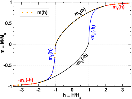
Figure 1: Piecewise parameterization of the SW hysteresis loop (orange dots) by functions $m_{1}$, $m_{2}$, and $m_{3}$ (colored lines).

II Parametrization

II.1 Direct $m(h)$

We approximate $m(h)$ by 3 analytic functions (Fig. 1):

$$m(h)=\left\{\begin{array}[]{c l }m_{1}(h),&h\in[2,+\infty);\\ m_{2}(h),&h\in[-1,2];\\ m_{3}(h),&h\in[-2,-1].\end{array}\right.$$ (1)

We denote $m_{0}\!\equiv\!m(-1)\!\approx\!-0.05284686$, see Table 1. The whole hysteresis loop can be constructed using the inversion symmetry, which transforms $m(h)\to-m(-h)$; for example, $m(h)=-m_{1}(-h)$ at $h\leq-2$. At $h=-1$, the first derivative $dm/dh$ is discontinuous and infinite for $m_{3}$, but $(m_{3}(h)-m_{0})^{2}$ has a finite slope for all $h\in[-2,-1]$, and we fit this squared function. At $h=2$, there is a well-known kink in the second derivative ${d^{2}m}/{dh^{2}}$, experimentally observed using the singular point detection techniques [34].

Table 1: Values of $m(h)$ and $\overline{\cos\phi}$ from SW [1].

$h$	$m(h)$	SW [1]
$-\infty$	$-$1	$-$1
$-$1	$-$0.05284686	$-$0.052631
0	$0.5$	0.5
1	0.7607696	0.760770
2	0.9129751	0.9130
3	0.9645663	0.9646
4	0.9809153	0.9809
$\infty$	1	1

Using machine learning, we perform a piecewise least-squares (LS) fit of the following functions (with coefficients in Table 2):

$$\left.\begin{aligned} m_{1}(h\geq 2)&=\frac{1+\sum_{n=1}^{3}c_{n}h^{-2n}}{1+d_{1}h^{-2}},\\ m_{2}(-1\!\leq\!h\!\leq\!2)\,&=\,\frac{0.5+\sum_{n=1}^{6}c_{n}h^{n}}{1+d_{1}h+d_{2}h^{2}},\\ m_{3}(-2\!\leq\!h\!\leq\!-1)&=m_{0}+\left[\frac{\sum_{n=1}^{3}c_{n}(-h-1)^{n}}{1+\sum_{k=1}^{3}d_{k}(-h-1)^{k}}\right]^{1/2}\end{aligned}\right.$$ (2)

These functions return $m_{1}(\infty)\equiv 1$, $m_{2}(0)\equiv 0.5$, and $m_{3}(-1)\equiv m_{0}$, see Fig. 1 and Table 1. Each function is accurate within its domain, see Appendix.

Table 2: Coefficients of eqs. 2 and accuracy of the fit: least-squares fit error $\chi^{2}$, Theil U, and correlation (C) coefficients.

	$m_{1}$	$m_{2}$	$m_{3}$
$c_{1}$	18.2445	1.20029	2.90821
$c_{2}$	-5.96049	0.854124	10.1974
$c_{3}$	-3.1374	0.116601	-5.12248
$c_{4}$	–	-0.031271	–
$c_{5}$	–	0.0045254	–
$c_{6}$	–	-0.00176557	–
$d_{1}$	18.5187	1.73361	4.01935
$d_{2}$	–	0.739904	13.3217
$d_{3}$	–	–	-7.55852
$\chi^{2}$	$5\times 10^{-7}$	$3\times 10^{-6}$	$2\times 10^{-4}$
U	$5\times 10^{-6}$	$4\times 10^{-5}$	$1\times 10^{-3}$
C	1.000000	1.000000	0.999995

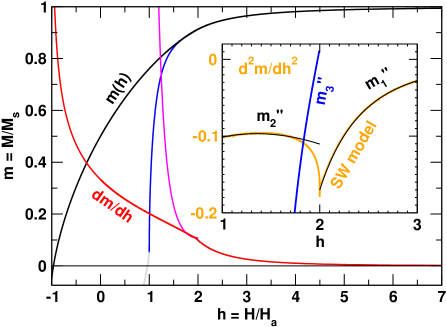
Figure 2: The SW model (increasing grey $m(h)$ lines), its first (decreasing orange $dm/dh$ in the plot), and second derivatives (orange $d^{2}m/dh^{2}$ lines in the inset), and our approximation by the analytic functions: black $m_{1}$ and $m_{2}$, blue $-m_{3}$, as well as their first (decreasing, same scale, red $m_{1}^{\prime}$ and $m_{2}^{\prime}$, pink $-m_{3}^{\prime}$ lines) and (inset) second derivatives (black $m_{1}^{\prime\prime}$ and $m_{2}^{\prime\prime}$, blue $-m_{3}^{\prime\prime}$ lines). Except for the second derivatives (inset), the SW model and the analytic functionals are indistinguishable, thus most of the gray and orange lines (SW model) are covered by the approximating lines.

II.2 Inverse $h(m)$

We also parametrize the inverse function by

$$h(m)=\left\{\begin{array}[]{c l }h_{+}(m>m_{0}),&h\in[-1,+\infty);\\ h_{-}(m\leq m_{0}),&h\in(-\infty,-1].\end{array}\right.$$ (3)

A single analytical function $h_{+}(m)$ in the first quadrant ignores a kink in $d^{2}m/dh^{2}$ at $h=2$, but covers both $m_{2}$ and $m_{1}$. Similarly, $h_{-}(m)$ is the inverse function for both $-m_{1}(-h)$ and $m_{3}(h)$, see Fig. 1.

First, we map $h\in(-\infty,+\infty)$ onto $y\in[0,1]$ using the transformation $y=1/[(h+1)^{2}+1]$, and piecewise fit $y(m)$ by two rational functions: one increasing and one decreasing. Next, we substitute those into the inverse transformation $h=-1+sqrt(abs(-1+1/y))$, where $sqrt(x)=\sqrt{x}$ is the square root and $abs(x)=|x|$ is the absolute value (needed only near $h=-1$). We get

$$h_{\pm}(m)=-1+\left|-1+\frac{1+\sum_{n=1}^{5}{c_{n}(m\mp 1)^{n}}}{\sum_{k=1}^{5}{d_{k}(m\mp 1)^{k}}}\right|^{1/2}$$ (4)

with coefficients in Table 3. Here $h_{+}$ is expanded in terms of $(m-1)$. The error in $y[h(m)]$ with $h_{\pm}(m)$ approximated by eq. 4 is below $6\times 10^{-4}$.

Table 3: Coefficients of eqs. 3, see Table 2 caption.

	$h_{+}$	$h_{-}$
$c_{1}$	-16.0382	-9.14903
$c_{2}$	33.7616	61.4734
$c_{3}$	106.516	-336.135
$c_{4}$	91.6034	0.290317
$c_{5}$	–	18813.8
$d_{1}$	-2.59778	4.55815
$d_{2}$	0.782093	0.577252
$d_{3}$	-43.4887	-357.282
$d_{4}$	-52.8431	209.511
$d_{5}$	-41.8217	18676.5
$\chi^{2}$	$7\times 10^{-5}$	0.0001
U	0.0004	0.0005
Corr.	1.000000	1.000000

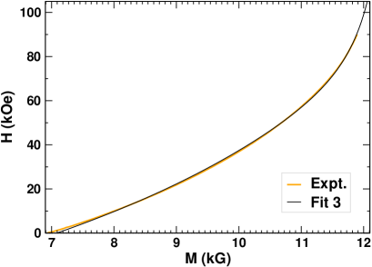
Figure 3: Experimental data (Expt., orange), fitted (Fit 3, black line) by 3-parameter eq. 5 at $H\!>\!0$.

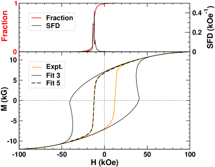
Figure 4: (Lower) Experimental M(H) data (Expt., orange lines), its 3-parameter fit (Fit 3, solid black lines) by the theoretical curves with demagnetization (eq. 5), and 5-parameter fit (Fit 5, dashed black line) with SFD approximated by eq. 6. (Upper) A fraction of the reversed magnetization (left scale, red) and its derivative (SFD: right scale, black).

III Application

Experiment. The magnetic hysteresis loop was measured for the ribbons of an Ames rare-earth magnetic alloy. To prepare the ribbons, ingots with composition (Nd_0.80Pr_0.20)₂Fe₁₄B were prepared by arc melting materials of constituent elements in argon atmosphere. Melt spun ribbons were prepared by inductively melting the ingots in quartz crucibles and ejecting the melt onto a single copper wheel at 30 m/s surface velocity through a 0.8 mm orifice. Melt spinning was performed in 1/3 atmosphere of high purity He gas. The as-spun ribbons were crystallized by heat treatment at 700^∘C for 15 min in 1/3 ultra-high purity argon atmosphere. Magnetic hysteresis loop was measured at 300 K in a Quantum Design vibrating sample magnetometer with maximum applied magnetic field of 90 kOe.

Analysis. Eq. 4 can be used to fit a measured data at $H\!>\!0$, taking into account demagnetization:

$$H(M)=H_{a}h_{+}(M/M_{s})-\bar{\gamma}M,$$ (5)

where $\bar{\gamma}=\gamma/4\pi$ is a demagnetizing factor. Using a sufficiently large initial guess of $M_{s}$ to avoid a singularity of $H(M)$ at $M=M_{s}$, we fit experimental $H(M)$ data at $H\!>\!0$ by 3 parameters ($H_{a}$, $M_{s}$, $\bar{\gamma}$) in eq. 5.

The result of fitting the measurements at $H>0$ by eq. 5 is in Fig. 3. We find $H_{a}=41.55\,$kOe, $M_{s}=12.54\,$kG, and $\bar{\gamma}=1.2$.

Due to the switching field, demagnetization data deviates from the SW model (or its parametrization) at $H<0$. A fraction of the reversed magnetization can be approximated by a sigmoid curve $S(x)$ with two parameters ($H_{S}$ and $\Delta H_{S}$) in the argument $x=(H-H_{S})/\Delta H_{S}$.

We use $S_{L}(x)=\frac{1}{2}(L(x)+1)$ with the classical Langevin function $L(x)=coth(x)-1/x$. Its first derivative is a bell-shaped curve:

$$S_{L}^{\prime}(H)\equiv\frac{dS_{L}}{dH}=\frac{1}{2}\frac{dL}{dx}\frac{dx}{dH}=\hfill$$ (6)

$$=\frac{1}{2\,\Delta H_{S}^{L}}\left[1-coth^{2}\left(\frac{H-H_{S}}{\Delta H_{S}^{L}}\right)+\left(\frac{\Delta H_{S}^{L}}{H-H_{S}}\right)^{2}\right]$$

Comparing the upper branch of the experimental $M(H)$ data to the two branches [$m(h)$ and $-m(-h)$] of the parametrized SW model, we get a fraction of the reversed magnetization, see Fig. 4. By fitting it to $S_{L}$, we get $H_{S}=-12.44\,$kOe and $\Delta H_{S}^{L}=0.484\,$kOe. Its derivative is the switching field distribution (SFD), which can be approximated by eq. 6.

IV Summary

We have provided a convenient analytic approximation for the Stoner-Wohlfarth model [1], suitable for quick and easily computations. We applied it to the measured magnetic hysteresis loop and fitted the experimental data by 5 parameters: $M_{s}$, $H_{a}$, $\bar{\gamma}$, $H_{S}$, and $\Delta H_{S}$. Our easy-to-compute analytic functions serve as useful tools for description of magnetic materials, that facilitate materials discovery [11; 35; 36; 37].

Appendix A Analysis of $m(h)$ fit and its derivatives

The fitted function $m(h)$ and its derivatives are shown in Fig. 2. Difference between $m(h)$ and its fit by the analytic functions $m_{n}$ ($n=1,2,3$) from eq. 2 is within the numeric noise. The first derivative of $m_{n}$ is indistinguishable from $dm/dh$ for the model. The inset in Fig. 2 shows that $d^{2}m/dh^{2}$ is reproduced well at $h>2$ or $h<1.7$, but not at $h=2-\delta$. The 2nd derivative of $m_{1}$ (at $h\geq 2$) coincides with the model, while $d^{2}m_{2}/dh^{2}$ deviates at $h=2-\delta$ for $0\leq\delta<0.3$, and the 2nd derivative of $-m_{3}(-h)$ (blue line in Fig. 2 inset) has a larger deviation near $h=2$.

The function $m(h)$ itself and its first derivative are reproduced very well everywhere, hence the lines for the SW model and its analytic approximation are indistinguishable in Fig. 2. The function $m_{1}(h)$ and its derivatives are as good as the tabulated values of $m(h)$ at $h\geq 2$. The largest error (calculated as a deviation from $m(h)$ at a given $h$) is $3\times 10^{-5}$ for $m_{1}$ at $h=2$ (it is $<\!1\times 10^{-5}$ for $h>2.537$ and $<1.34\times 10^{-5}$ for $h>2.066$); 0.001 for $m_{3}$ at h=0 ($<0.0005$ at $0.12<h<1$); and 0.0008 for $m_{2}$ at $h=-1$ (0.0001 at h=2, and $\leq\!1\!\times\!10^{-4}$ at $-0.986<h\leq 2$).

The first derivative at $h=2$ is $m^{\prime}(2)\equiv dm/dh|_{h=2}=0.09869$ for the model. The error in $m^{\prime}(2)$ constitutes 0.00037 for $m_{1}^{\prime}$, 0.003 for $m_{2}^{\prime}$, and 0.01 for $m_{3}^{\prime}$. This error in $dm/dh$ is the largest for $m_{1}^{\prime}$ and $m_{3}^{\prime}$, while $dm_{2}/dh$ has a smaller error $\leq 0.001$ at $-0.8<h<1.9$, but an expectedly large error exceeding 0.01 near $h=-1$.

The second derivative $m_{1}^{\prime\prime}\equiv d^{2}m_{1}/dh^{2}$ reproduces the model correctly in the whole domain of $m_{1}$ at $h\in[2,+\infty)$, see Fig. 2 inset. However, $m_{2}^{\prime\prime}$ and $m_{3}^{\prime\prime}$ deviate from the model at $h=2-\delta$, where $0\leq\delta<0.3$. At $h=2$, this deviation reaches 0.006 for $m_{1}^{\prime\prime}$, 0.06 for $m_{2}^{\prime\prime}$, and 0.19 for $m_{3}^{\prime\prime}$ second derivative, where $m^{\prime\prime}(2)\equiv d^{2}m/dh^{2}|_{h=2}\approx-0.18$ for the model, see Fig. 2 inset. If needed, the second derivative $d^{2}m/dh^{2}$ at $-1<h\leq 2$ can be directly approximated by eq. (7):

$$m_{(2)}^{\prime\prime}=-0.303321\,(h+1)^{-1}-0.156365-0.049342\,h$$

$$+0.0893185\,h^{2}-0.0458726\,h^{3}+0.0118055\,h^{4}$$

$$+0.148387\,(2-h)^{1/2}+0.0524192\,(2-h)^{1/4},$$

which is accurate even at $h=2-\delta$. The function $m_{(2)}\equiv\int\int m_{(2)}^{\prime\prime}$, obtained by double integration of $m_{(2)}^{\prime\prime}(h)$ at $-1<h\leq 2$, contains roots and a logarithm, which are slower to compute.

Equations 2 and A provide accurate analytic expressions for $m(h)$ function and its 1st and 2nd derivatives (a luxury, not offered by DLN), while the inverse function $h(m)$ in eq. 4 facilitates a fit of experimental data.

References

- E. C. Stoner and E. P. Wohlfarth [1948] E. C. Stoner and E. P. Wohlfarth, Philosophical Transactions of the Royal Society A 240, 599 (1948).
- R. W. McCallum [2005] R. W. McCallum, Journal of Magnetism and Magnetic Materials 292, 135 (2005).
- Zarkevich [2006] N. A. Zarkevich, Complexity 11, 36 (2006).
- Pizzi et al. [2016] G. Pizzi, A. Cepellotti, R. Sabatini, N. Marzari, and B. Kozinsky, Computational Materials Science 111, 218 (2016).
- Saal et al. [2013] J. E. Saal, S. Kirklin, M. Aykol, B. Meredig, and C. Wolverton, JOM 65, 1501 (2013).
- Zhang and Ling [2018] Y. Zhang and C. Ling, npj Computational Materials 4, 25 (2018).
- Raccuglia et al. [2016] P. Raccuglia, K. C. Elbert, P. D. F. Adler, C. Falk, M. B. Wenny, A. Mollo, M. Zeller, S. A. Friedler, J. Schrier, and A. J. Norquist, Nature 533, 73 (2016).
- Zarkevich and Johnson [2004] N. A. Zarkevich and D. D. Johnson, Phys. Rev. Lett. 92, 255702 (2004).
- Zarkevich and Johnson [2003] N. A. Zarkevich and D. D. Johnson, Phys. Rev. B 67, 064104 (2003).
- Zarkevich et al. [2002] N. A. Zarkevich, D. D. Johnson, and A. V. Smirnov, Acta Materialia 50, 2443 (2002).
- Zarkevich et al. [2017] N. A. Zarkevich, D. D. Johnson, and V. K. Pecharsky, Journal of Physics D: Applied Physics 51, 024002 (2017).
- Zarkevich and Johnson [2016] N. A. Zarkevich and D. D. Johnson, Phys. Rev. B 93, 020104 (2016).
- Zarkevich and Johnson [2005] N. A. Zarkevich and D. D. Johnson, Surface Science 591, L292 (2005).
- Xu et al. [2005] G. J. Xu, N. A. Zarkevich, A. Agrawal, A. W. Signor, B. R. Trenhaile, D. D. Johnson, and J. H. Weaver, Phys. Rev. B 71, 115332 (2005).
- Zarkevich and Johnson [2008] N. A. Zarkevich and D. D. Johnson, Phys. Rev. Lett. 100, 040602 (2008).
- Zarkevich et al. [2007] N. A. Zarkevich, T. L. Tan, and D. D. Johnson, Phys. Rev. B 75, 104203 (2007).
- Zarkevich et al. [2008] N. A. Zarkevich, T. L. Tan, L.-L. Wang, and D. D. Johnson, Phys. Rev. B 77, 144208 (2008).
- Zarkevich et al. [2014a] N. A. Zarkevich, E. H. Majzoub, and D. D. Johnson, Phys. Rev. B 89, 134308 (2014a).
- Zarkevich and Johnson [2015a] N. A. Zarkevich and D. D. Johnson, J. Chem. Phys. 142, 024106 (2015a).
- Zarkevich and Johnson [2019] N. A. Zarkevich and D. D. Johnson, J. Alloys Compd. 802, 712 (2019).
- Zarkevich et al. [2014b] N. A. Zarkevich, L.-L. Wang, and D. D. Johnson, APL Materials 2, 032103 (2014b).
- Zarkevich and Johnson [2015b] N. A. Zarkevich and D. D. Johnson, Phys. Rev. B 91, 174104 (2015b).
- Zarkevich and Johnson [2015c] N. A. Zarkevich and D. D. Johnson, J. Chem. Phys. 143, 064707 (2015c).
- Zarkevich and Johnson [2018] N. A. Zarkevich and D. D. Johnson, Phys. Rev. B 97, 014202 (2018).
- S. V. Vonsovskii [1971] S. V. Vonsovskii, Magnetism (Nauka, Moscow, 1971) in Russian. Translated: Wiley (1974), ISBN 047091193X.
- Ivahnenko and Lapa [1965] A. G. Ivahnenko and V. G. Lapa, Kiberneticheskie predskazyvayuschie ustrojstva (Naukova Dumka, Kiev, 1965) in Russian.
- Goodfellow et al. [2016] I. Goodfellow, Y. Bengio, and A. Courville, Deep Learning (MIT Press, 2016).
- Russell and Norvig [2016] S. Russell and P. Norvig, Artificial Intelligence: A Modern Approach, 3rd ed. (Pearson, 2016).
- A.G. Stoletov [1873] A.G. Stoletov, Lon. E. Dublin Phil. Mag. J. Sci. 45, 40 (1873), translated from Pogg. Ann. 144, 439–463 (1871). Presented before the Moscow Mathematical Society on 20 Nov (2 Dec) 1871.
- W. Tang, K.W. Dennis, Y.Q. Wu, M.J. Kramer, I.E. Anderson, and R.W. McCallum [2004] W. Tang, K.W. Dennis, Y.Q. Wu, M.J. Kramer, I.E. Anderson, and R.W. McCallum, IEEE Trans. Magn. 40, 2907 (2004).
- M. Huang, D. Wu, K.W. Dennis, J.W. Anderegg, R.W. McCallum, and T.A. Lograsso [2005] M. Huang, D. Wu, K.W. Dennis, J.W. Anderegg, R.W. McCallum, and T.A. Lograsso, J. Phase Equilib. Diffusion 26, 209 (2005).
- S.H. Song, D.C. Jiles, J.E. Snyder, A.O. Pecharsky, D. Wu, K.W. Dennis, T.A. Lograsso, and R.W. McCallum [2005] S.H. Song, D.C. Jiles, J.E. Snyder, A.O. Pecharsky, D. Wu, K.W. Dennis, T.A. Lograsso, and R.W. McCallum, J. Appl. Phys. 97, 10M516 (2005).
- Pecharsky et al. [2003] A. O. Pecharsky, Y. Mozharivskyj, K. W. Dennis, K. A. Gschneidner, R. W. McCallum, G. J. Miller, and V. K. Pecharsky, Phys. Rev. B 68, 134452 (2003).
- Bolzoni and Cabassi [2004] F. Bolzoni and R. Cabassi, Physica B 346–347, 524 (2004).
- Yibole et al. [2018] H. Yibole, A. Pathak, Y. Mudryk, F. Guillou, N. A. Zarkevich, S. Gupta, V. Balema, and V. K. Pecharsky, Acta Materialia 154, 365 (2018).
- Bez et al. [2019] H. N. Bez, A. K. Pathak, A. Biswas, N. A. Zarkevich, V. Balema, Y. Mudryk, D. D. Johnson, and V. K. Pecharsky, Acta Materialia 173, 225 (2019).
- Biswas et al. [2019] A. Biswas, A. K. Pathak, N. A. Zarkevich, X. Liu, Y. Mudryk, V. Balema, D. D. Johnson, and V. K. Pecharsky, Acta Materialia 180, 341 (2019).