Dependent Modeling of Temporal Sequences of Random Partitions

Abstract

We consider modeling a dependent sequence of random partitions. It is well-known in Bayesian nonparametrics that a random measure of discrete type induces a distribution over random partitions. The community has therefore assumed that the best approach to obtain a dependent sequence of random partitions is through modeling dependent random measures. We argue that this approach is problematic and show that the random partition model induced by dependent Bayesian nonparametric priors exhibits counter-intuitive dependence among partitions even though the dependence for the sequence of random probability measures is intuitive. Because of this, we suggest directly modeling the sequence of random partitions when clustering is of principal interest. To this end, we develop a class of dependent random partition models that explicitly models dependence in a sequence of partitions. We derive conditional and marginal properties of the joint partition model and devise computational strategies when employing the method in Bayesian modeling. In the case of temporal dependence, we demonstrate through simulation how the methodology produces partitions that evolve gently and naturally over time. We further illustrate the utility of the method by applying it to an environmental data set that exhibits spatio-temporal dependence.

Keywords: correlated partitions; hierarchical Bayes modeling; Bayesian nonparametrics; spatio-temporal clustering.

1 Introduction

We introduce a method to directly model dependence in a sequence of random partitions. Our approach is motivated by the practical problem of defining a prior distribution to model a sequence of random partitions that potentially exhibits substantial concordance over time (e.g., gently evolving clusterings over time). Traditionally, dependencies in random partitions (i.e., the clustering of units) have been obtained as a by-product of dependent random measures in Bayesian nonparametric (BNP) methods. We argue, however, that when a sequence of partitions is the inferential object of interest, then the sequence of partitions should be modeled directly rather than relying on induced random partition models, such as those implied by temporally dependent BNP models. But first, we review the literature on dependent BNP methods.

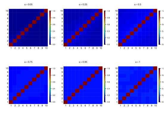
Figure 1: For various values of the temporal dependence parameter $\alpha$, these plots show the lagged ARI values using the method of Caron et al. (2017) based on concentration parameter $M=0.5$, discount parameter set to zero, and 10,000 Monte Carlo samples.

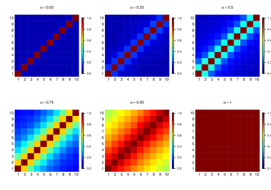
Figure 2: Lagged ARI values based on 10,000 Monte Carlo samples using the method developed in this paper. Partitions show natural and intuitive temporal dependence as lagged time increases and as the temporal dependence parameter $\alpha$ increases.

A non-exhaustive list of Bayesian nonparametric methods that temporally correlate a sequence of random probability measures include Nieto-Barajas et al. (2012), Antoniano-Villalobos and Walker (2016), Gutiérrez et al. (2016), Jo et al. (2017), Kalli and Griffin (2018), DeYoreo and Kottas (2018), and De Iorio et al. (2019). A common aspect of all these methods is that temporal dependence is accommodated in the sequence of random measures by way of the atoms or weights of the stick-breaking representation (Sethuraman, 1994). An alternative approach to producing a sequence of temporally correlated random probability measures can be found in Caron et al. (2007) and Caron et al. (2017). Their construction is based on a generalised Pólya urn scheme where dependencies between distributions that evolve over time are induced by urn-like operations on counts and the parameters to which they are associated. A key insight associated with all mentioned approaches, however, is that the induced random partitions only exhibit weak dependence even when a sequence of random probability measures is highly correlated. To illustrate this point, we conducted a small Monte Carlo simulation where an induced sequence of partitions was generated with 10 time points and 20 units using the method of Caron et al. (2017). To measure similarity of partitions at different time points, we use a time-lagged adjusted Rand index (ARI) (Hubert and Arabie 1985). Figure 1 shows these values averaged over 10,000 Monte Carlo samples. Notice that as the temporal dependence parameter ($\alpha$) increases, the partitions from time period $t$ to $t+1$ only become slightly more similar, such that the dependence between partitions is, at best, only weak. Further, the dependence is not temporally intuitive as it does not decay as a function of lagged time. In contrast, compare the dependence structure in Figure 1 to that in Figure 2, which contains average lagged ARI values between time lagged partitions generated using the method developed in this paper. Notice that unlike the induced random partitions generated using the method in Caron et al. (2017), the sequence of partitions generated using our approach displays intuitive temporal dependence. That is, as the time lag increases, similarity between partitions decreases and as the temporal dependence parameter $\alpha$ increases, the partitions become dissimilar over time at a slower rate.

The counter-intuitive behavior displayed in Figure 1 is not unique to the approach of Caron et al. (2017). As noted by Wade et al. (2014), the same type of behavior is present when using a linear dependent Dirichlet process mixture model. In fact, all BNP methods that model a sequence of discrete random probability measures will induce a random partition model with similarly weak correlation behavior. This behavior is analogous to trying to induce dependence among random variables from distributions with correlated parameters. There is no guarantee that correlated parameters would produce strong correlations among the random variables themselves.

Our approach is to consider the sequence of partitions as the parameter of principal interest and develop a method that models it directly. This will provide more control over how “smoothly” partitions evolve over time. Perhaps the work closest to ours, in the sense of explicitly modeling a sequence of partitions, can be found in Zanini et al. (2019). Their modeling approach for a temporally-referenced sequence of partitions can be applied to only two time points and differs from ours in that they do not focus on smooth evolution of partitions over time.

The remainder of the article is organized as follows. In Section 2 we present the proposed approach for a sequence of dependent random partitions, discuss its main properties, and suitable computational strategies for inference based on posterior simulation. Section 3 contains the results from three simulation studies that further explore aspects of the model. Section 4 describes an environmental data application and some concluding remarks are provided in Section 5. An accompanying Supplementary Materials file collects the proofs of results stated below, provides details on posterior simulation algorithms, and contains further simulation and data analysis results.

2 Joint Model for a Sequence of Partitions

Before detailing our method, we introduce some general notation. Let $i=1,\ldots,m$ denote the $m$ experimental units at time $t$ for $t=1,\ldots,T$. Let $\rho_{t}=\{S_{1t},\ldots,S_{k_{t}t}\}$ denote a partition of the $m$ experimental units at time $t=1,\ldots,T$ into $k_{t}$ clusters. An alternative notation is based on $m$ cluster labels at time $t$ denoted by $\bm{c}_{t}=\{c_{1t},\ldots,c_{mt}\}$ where $c_{it}=j$ implies that $i\in S_{jt}$. Finally, any quantity with a “$\star$” superscript will be cluster-specific. For example, we will use $\mu^{\star}_{jt}$ to denote the mean of cluster $j$ at time $t$ so that $\mu_{it}=\mu^{\star}_{c_{it}t}$.

2.1 Temporal Modeling for Sequences of Partitions

Introducing temporal dependence in a collection of partitions requires formulating a joint probability model for $(\rho_{1},\ldots,\rho_{T})$. Generically, we will denote this joint model with $\text{Pr}(\rho_{t},\ldots,\rho_{T})$. Temporal dependence among the $\rho_{t}$’s implies that the cluster configuration in $\rho_{t}$ could be impacted by that found in $\rho_{t-1},\rho_{t-2},\ldots,\rho_{1}$. However, we assume that the probability model for the sequence of partitions has a first-order Markovian structure. That is, the conditional distribution of $\rho_{t}$ given $\rho_{t-1},\rho_{t-2},\ldots,\rho_{1}$ only depends on $\rho_{t-1}$. Thus, we construct $\text{Pr}(\rho_{t},\ldots,\rho_{T})$ as

$$\text{Pr}(\rho_{1},\ldots,\rho_{T})=\text{Pr}(\rho_{T}\mid\rho_{T-1})\text{Pr}(\rho_{T-1}\mid\rho_{T-2})\cdots\text{Pr}(\rho_{2}\mid\rho_{1})\text{Pr}(\rho_{1}).$$ (1)

Here $\text{Pr}(\rho_{1})$ is an exchangeable partition probability function (EPPF) that describes how the $m$ experimental units at time period 1 are grouped into $k_{1}$ distinct groups with frequencies $n_{11},\ldots,n_{1k_{1}}$. One characteristic of an EPPF that will prove useful in what follows is sample size consistency, or what De Blasi et al. (2015) refer to as the addition rule. This property dictates that marginalizing the last of $m+1$ elements leads to the same model as if we only had $m$ elements. A commonly encountered EPPF is that induced by a Dirichlet process (DP). This particular EPPF is sometimes referred to as a Chinese restaurant process (CRP) which can be seen as a special case from the family of product partition models (PPM). For more details, see De Blasi et al. (2015). Because we employ the EPPF of the CRP in what follows, we provide its form here

$$\text{Pr}(\rho\mid M)=\frac{M^{k}}{\prod_{i=1}^{n}(M+i-1)}\prod_{i=1}^{k}(|S_{i}|-1)!,$$ (2)

where $k$ is the number of clusters in $\rho$ and $M$ is a concentration parameter controlling the number of clusters. We will denote this random partition distribution as $CRP(M)$.

Although conceptually straightforward, (1) is silent regarding how $\rho_{t-1}$ influences the form of $\rho_{t}$. To make this explicit, we introduce an auxiliary variable that guides the similarity between $\rho_{t}$ and $\rho_{t-1}$. Note that if two partitions are highly dependent, then the cluster configurations between them will change very little and as a result only a few of the $m$ experimental units will change cluster assignment. Conversely, two partitions that exhibit low dependence will likely be comprised of very different cluster configurations. The auxiliary variable we introduce identifies which of the experimental units at time $t-1$ will be considered for possible cluster reallocation at time $t$. Specifically, let $\gamma_{it}$ denote the following

$$\gamma_{it}=\left\{\begin{array}[]{c l}1&\mbox{if unit $i$ is {\it not} reallocated when moving from time $t-1$ to $t$}\\ 0&\mbox{otherwise},\end{array}\right.$$ (5)

for $i=1,\ldots,m$. Notice that when $\gamma_{it}=0$, item $i$ is subject to reallocation at time $t$, but still may, by random assignment, end up in the same cluster at time $t$ as it was at time $t-1$. By construction, we set $\gamma_{i1}=0$ for all $i$, i.e., all experimental units are allocated to clusters during the first time period. We then assume that $\gamma_{it}\stackrel{{\scriptstyle ind}}{{\sim}}Ber(\alpha_{t})$. Note that each of the $\alpha_{t}\in[0,1]$ acts as a temporal dependence parameter. Specifically, we will interpret $\alpha_{t}=1$ as implying that $\rho_{t}=\rho_{t-1}$ with probability 1. Conversely, when $\alpha_{t}=0$, then $\rho_{t}$ is independent of $\rho_{t-1}$. Further, when $\alpha_{t}$ is constant for all $t$, the degree of dependence among partitions is constant over time, whereas general values for $\alpha_{t}$ provide for varying degrees of dependence and more flexible partition patterns over time. For notational convenience, we introduce $\bm{\gamma}_{t}=(\gamma_{1t},\gamma_{2t},\ldots,\gamma_{mt})$ which is an $m$-tuple comprised of zeros and ones. The augmented joint model changes (1) to

$$\text{Pr}(\bm{\gamma}_{1},\rho_{1},\ldots,\bm{\gamma}_{T},\rho_{T})=\text{Pr}(\rho_{T}\mid\bm{\gamma}_{T},\rho_{T-1})\text{Pr}(\bm{\gamma}_{T})\times\\ \text{Pr}(\rho_{T-1}\mid\bm{\gamma}_{T-1},\rho_{T-2})\text{Pr}(\bm{\gamma}_{T-1})\cdots\text{Pr}(\rho_{2}\mid\bm{\gamma}_{2},\rho_{1})\text{Pr}(\bm{\gamma}_{2})\text{Pr}(\rho_{1}).$$ (6)

We describe $\text{Pr}(\rho_{t}\mid\bm{\gamma}_{t},\rho_{t-1})$ shortly, but first provide a definition.

Definition 1.

We say that partitions $\rho_{t-1}$ and $\rho_{t}$ are compatible with respect to $\bm{\gamma}_{t}$, if $\rho_{t}$ may be obtained from $\rho_{t-1}$ by reallocating items as indicated by $\bm{\gamma}_{t}$, i.e., those items $i$ such that $\gamma_{ti}=0$ for $i=1,\ldots,m$. Note that the compatibility relation is an equivalence relation.

There is a simple way to check if $\rho_{t-1}$ is compatible with $\rho_{t}$ with respect to $\bm{\gamma}_{t}$. Let $\mathfrak{R}_{t}=\{i:\gamma_{it}=1\}$ be the collection of units that remain fixed when moving from time $t-1$ to time $t$, and $\mathfrak{R}^{C}_{t}=\{i:\gamma_{it}=0\}$ is the collection of units that do not. Next denote with $\rho^{\mathfrak{R}_{t}}_{t}$ the “reduced” partition at time $t$ that remains after removing all items in $\mathfrak{R}^{C}_{t}$ from the subsets of $\rho_{t}$. Similarly, let $\rho^{\mathfrak{R}_{t}}_{t-1}$ be the reduced partition at time $t-1$ based on $\bm{\gamma}_{t}$. Then $\rho_{t-1}$ and $\rho_{t}$ are compatible with respect to $\bm{\gamma}_{t}$ if and only if $\rho^{\mathfrak{R}_{t}}_{t-1}=\rho^{\mathfrak{R}_{t}}_{t}$.

Now, to further characterize $\text{Pr}(\rho_{t}\mid\bm{\gamma}_{t},\rho_{t-1})$, let $P$ denote the set of all partitions of $m$ units and let $P_{C_{t}}=\{\rho_{t}\in P:\rho^{\mathfrak{R}_{t}}_{t-1}=\rho^{\mathfrak{R}_{t}}_{t}\}$ be the collection of partitions at time $t$ that are compatible with $\rho_{t-1}$ based on $\bm{\gamma}_{t}$. Then, by construction, $\text{Pr}(\rho_{t}\mid\bm{\gamma}_{t},\rho_{t-1})$ is a random partition distribution whose support is $P_{C_{t}}$ so that

$$\text{Pr}(\rho_{t}=\lambda\mid\bm{\gamma}_{t},\rho_{t-1})=\displaystyle\frac{\text{Pr}(\rho_{t}=\lambda)\text{I}[\lambda\in P_{C_{t}}]}{\sum_{\lambda^{\prime}}\text{Pr}(\rho_{t}=\lambda^{\prime})\text{I}[\lambda^{\prime}\in P_{C_{t}}]},$$

where $\text{Pr}(\rho_{t}=\lambda)$ is the EPPF at the first time point evaluated at $\lambda$. Here, and in what follows, $\text{I}[A]$ denotes an indicator function with $\text{I}[A]=1$ if statement $A$ is true, and $0$ otherwise.

It would be appealing if marginally each of the $\rho_{t}$ follow the assumed EPPF for $\rho_{1}$, so that the joint probability model for partitions would be stationary. The following proposition establishes this result, which is a consequence of the fact that conditioning on $\bm{\gamma}_{t}$ provides a “reduced” EPPF.

Proposition 1.

Let $\rho_{1}\sim EPPF$ and $\bm{\gamma}_{1}=\bm{0}$. If a joint model for $\rho_{1}\ldots,\rho_{T}$ is constructed as described above by introducing $\bm{\gamma}_{t}$ for $t=2,\ldots,T$, then we have that marginally $\rho_{1},\ldots,\rho_{T}$ are identically distributed with law coming from the EPPF used to model $\rho_{1}$. Specifically, letting $\rho_{-t}=(\rho_{1},\ldots,\rho_{t-1},\rho_{t+1},\ldots,\rho_{T})$ and $\bm{\gamma}=(\gamma_{1},\ldots,\gamma_{T})$, we have that for all $\lambda\in P$,

$$\textup{Pr}(\rho_{t}=\lambda)=\sum_{\rho_{-t}\in P^{\otimes m}}\sum_{\bm{\gamma}\in\Gamma^{\otimes m}}\textup{Pr}(\bm{\gamma}_{1},\rho_{1},\ldots,\rho_{t}=\lambda,\ldots,\bm{\gamma}_{T},\rho_{T})=\textup{Pr}(\rho_{1}=\lambda),$$

where $P^{\otimes m}=P\times P\times\ldots\times P$, $P$ a collection of all partitions of $m$ units, $\Gamma^{\otimes m}=\Gamma\times\Gamma\times\ldots\times\Gamma$, and $\Gamma$ a collection of all possible binary vectors of size $m$.

Proof.

See supplementary material. ∎

In what follows, we will use $tRPM(\bm{\alpha},M)$ to denote our temporal random partition model (6) parameterized by $\alpha_{1},\ldots,\alpha_{T}$ and the EPPF in (2). We briefly mention that introducing $\gamma_{it}$ is similar in spirit to the approach taken by Caron et al. (2007); Caron et al. (2017). However, they use $\bm{\gamma}_{t}$ to identify a partial partition at time $t$ that informs how all the observational units will be reallocated at time $t+1$. While this difference may seem inconsequential at first glance, it has drastic ramifications on the type of dependence that exists among the actual sequence of partitions. This is illustrated in Figures 1 and 2 provided in the Introduction. The sequence of partitions used to create Figure 2 were generated using the $tRPM(\bm{\alpha},M)$ with $M=0.5$. As mentioned in the Introduction, when the main emphasis is on modeling a “smoothly” evolving sequence of random partitions, the temporal dependence displayed in Figure 2 is much more natural than that found in Figure 1.

2.2 Dependence in Partitions

We now further explore how our method models dependence across partitions. To do this, we analyze closeness between partitions $\rho_{1}$ and $\rho_{2}$ by way of co-clustering of cluster labels $(c_{11},\ldots,c_{m1})$ and $(c_{12},\ldots,c_{m2})$, respectively. We base our exploration on the Rand index which is defined a

$$R(\rho_{1},\rho_{2})=\frac{a+b}{\binom{m}{2}},$$

where $a$ is the number of pairs $(i,j)$ with $i,j\in[m]=\{1,\ldots,m\}$ that simultaneously co-cluster in $\rho_{1}$ and $\rho_{2}$ and $b$ is the number of such pairs that simultaneously do not co-cluster. Writing $\varphi_{ij}=P(c_{i1}=c_{j1},c_{i2}=c_{j2})+P(c_{i1}\neq c_{j1},c_{i2}\neq c_{j2})$, we note that

$$E\left[R(\rho_{1},\rho_{2})\right]=\binom{m}{2}^{-1}\sum_{1\leq i<j\leq m}\varphi_{ij}.$$

To provide context to the co-clustering probabilities of cluster labels based on $tRPM(\alpha,M)$, we consider the model proposed in Caron et al. (2007). In their approach and assuming $\rho_{1}\sim CRP(M)$, each $i\in[m]$ is randomly removed from the partition with probability $1-\alpha$, and $\rho_{2}$ is formed by running an extra $CRP(M)$ process, but starting from an urn that has weights given by the normalized cluster sizes left from the removal process. See details in Caron et al. (2007). We denote partitions that follow the model of Caron et al. (2007) as $\rho_{1},\rho_{2}\sim CAR(\alpha,M)$. For both our method and $CAR(\alpha,M)$, the case that $\alpha=0$ leads to $\rho_{1},\rho_{2}\stackrel{{\scriptstyle iid}}{{\sim}}CRP(M)$, while the largest degree of dependence between $\rho_{1}$ and $\rho_{2}$ is achieved when $\alpha=1$. The following proposition characterizes the co-clustering probabilities under our method and $CAR(\alpha,M)$.

Proposition 2.

Let $m=T=2$, so that $E\left[R(\rho_{1},\rho_{2})\right]=\varphi_{12}$.

• If $\rho_{1},\rho_{2}\sim tRPM(\alpha,M)$, where to simplify notation we write $\alpha\equiv\alpha_{2}$, then

  $$\varphi_{12}=\alpha^{2}+\frac{(1+M^{2})}{(1+M)^{2}}(1-\alpha)^{2}.$$

• If $\rho_{1},\rho_{2}\sim CAR(\alpha,M)$ then

  $$\varphi_{12}=\left[\frac{6+3M+4M^{2}+M^{3})}{(M+1)(M+2)(M+3))}\right]\alpha^{2}+\frac{(1+M^{2})}{(1+M)^{2}}\left(1-\alpha^{2}\right).$$

Proof.

See supplementary material. ∎

An interesting consequence of Proposition 2 is that we can compute the expected value of the Rand index in the case $\rho_{1},\rho_{2}\stackrel{{\scriptstyle iid}}{{\sim}}CRP(M)$.

Corollary 1.

If $\rho_{1},\rho_{2}\stackrel{{\scriptstyle iid}}{{\sim}}CRP(M)$ then for any $m\geq 2$,

$$E\left[R(\rho_{1},\rho_{2})\right]=\frac{(1+M^{2})}{(1+M)^{2}}.$$

Proof.

The result follows immediately by noting that the i.i.d. case coincides with $tRPM(0,M)$ and that by exchangeability and independence, $\varphi_{ij}=\varphi_{12}$ for all $1\leq i<j\leq m$. ∎

The result from Proposition 2 (a) shows that, under the $tRPM(\alpha,M)$ model, $\lim_{\alpha\rightarrow 0^{+}}\varphi_{12}=\frac{(1+M^{2})}{(1+M)^{2}}$, i.e., it agrees with $E\left[R(\rho_{1},\rho_{2})\right]$ under the i.i.d. case. The same holds as $\alpha\rightarrow 0^{+}$ under the $CAR(\alpha,M)$ model. Furthermore, for the $tRPM(\alpha,M)$, we get the appealing result that $\lim_{\alpha\rightarrow 1^{+}}\varphi_{12}=1$, but the same limit under the $CAR(\alpha,M)$ is a number strictly less than $1$ for any $M>0$. This reveals that the closeness between partitions under the proposed $tRPM(\alpha,M)$, as measured by the $\varphi_{12}$ quantity, can attain its maximum value of 1, which simply corresponds to the case where none of the units is relocated. The same cannot hold for the $CAR(\alpha,M)$ model because partitions are linked through a latent mechanism rather than directly as in the proposed model. Finally, we conjecture that similar results can be obtained for $m>2$ but calculations become more involved. The result from Corollary 1 is nevertheless valid for any $m\geq 2$.

2.3 Toy Example to Illustrate Conditional Model

To build intuition regarding the transition from $\rho_{t-1}$ to $\rho_{t}$, consider the conditional probabilities in equation (6) and the very simple scenario of $m=3$ and $T=2$. We have that

$$\text{Pr}(\rho_{2}\mid\rho_{1})=\sum_{\bm{\gamma}_{2}\in\Gamma}\text{Pr}(\rho_{2}\mid\bm{\gamma}_{2},\rho_{1})\text{Pr}(\bm{\gamma}_{2}),$$

where again, $\Gamma$ is the collection of all possible binary $3$-tuples and operate under $\rho_{1}\sim CRP(M)$. The conditional probabilities are provided in Table 1, where we set $M=1$ for simplicity. From Table 1, notice that $\text{Pr}(\rho_{2}\mid\rho_{1})$ is a reweighted CRP and that, as $\alpha\rightarrow 0$, partition probabilities correspond to those from the original CRP and, as $\alpha\rightarrow 1$, $\text{Pr}(\rho_{2}=\rho_{1})\rightarrow 1$. Further, notice that partitions associated with $\rho_{2}$ that are more similar to $\rho_{1}$ are given larger weight relative to a CRP. For example, given $\rho_{1}=\{\{1,2,3\}\}$ then $\rho_{2}=\{\{1,2\},\{3\}\}$ has higher probability than $\rho_{2}=\{\{1\},\{2\},\{3\}\}$ for any $\alpha>0$ but have equal probability in a CRP. From this toy example we see that the conditional co-clustering probabilities display dependencies in line with the desire to have partitions evolve gently over time.

Table 1: Partition probabilities from the conditional distribution $\text{Pr}(\rho_{2}\mid\rho_{1})$ using a CRP EPPF

$(c_{1},c_{2},c_{3})$	$\text{Pr}(\rho_{1})$	$\text{Pr}(\rho_{2}\mid\rho_{1}=a)$	$\text{Pr}(\rho_{2}\mid\rho_{1}=b)$	$\text{Pr}(\rho_{2}\mid\rho_{1}=c)$	$\text{Pr}(\rho_{2}\mid\rho_{1}=d)$	$\text{Pr}(\rho_{2}\mid\rho_{1}=e)$
$a=(1,1,1)$	$\frac{2}{6}$	$\frac{2}{6}[1+3\alpha^{2}-\alpha^{3}]$	$\frac{2}{6}[1-\alpha^{2}]$	$\frac{2}{6}[1-\alpha^{2}]$	$\frac{2}{6}[1-\alpha^{2}]$	$\frac{2}{6}[1-3\alpha^{2}+2\alpha^{3}]$
$b=(1,1,2)$	$\frac{1}{6}$	$\frac{1}{6}[1-\alpha^{2}]$	$\frac{1}{6}[1+3\alpha^{2}+2\alpha^{3}]$	$\frac{1}{6}[1-\alpha^{2}]$	$\frac{1}{6}[1-\alpha^{2}]$	$\frac{1}{6}[1+\alpha^{2}-2\alpha^{3}]$
$c=(1,2,1)$	$\frac{1}{6}$	$\frac{1}{6}[1-\alpha^{2}]$	$\frac{1}{6}[1-\alpha^{2}]$	$\frac{1}{6}[1+3\alpha^{2}+2\alpha^{3}]$	$\frac{1}{6}[1-\alpha^{2}]$	$\frac{1}{6}[1+\alpha^{2}-2\alpha^{3}]$
$d=(1,2,2)$	$\frac{1}{6}$	$\frac{1}{6}[1-\alpha^{2}]$	$\frac{1}{6}[1-\alpha^{2}]$	$\frac{1}{6}[1-\alpha^{2}]$	$\frac{1}{6}[1+3\alpha^{2}+2\alpha^{3}]$	$\frac{1}{6}[1+\alpha^{2}-2\alpha^{3}]$
$e=(1,2,3)$	$\frac{1}{6}$	$\frac{1}{6}[1-3\alpha^{2}+2\alpha^{3}]$	$\frac{1}{6}[1+\alpha^{2}-2\alpha^{3}]$	$\frac{1}{6}[1+\alpha^{2}-2\alpha^{3}]$	$\frac{1}{6}[1+\alpha^{2}-2\alpha^{3}]$	$\frac{1}{6}[1+3\alpha^{2}+2\alpha^{3}]$

2.4 Hierarchical Data Model

Once a partition model is specified, there is tremendous flexibility regarding how to model time (global or cluster-specific) at different levels of a hierarchical model (at the data level, process level, or both). Since we are interested to see how including time in the partition model impacts clustering and model fits, in the simulations of Section 3, we consider a hierarchical model where time only appears in the partition model. In particular, using cluster label notation, we will employ the following hierarchical model

$$Y_{it}\mid\bm{\mu}^{\star}_{t},\bm{\sigma}_{t}^{2\star},\bm{c}_{t} \stackrel{{\scriptstyle ind}}{{\sim}}N(\mu^{\star}_{c_{it}t},\sigma_{c_{it}t}^{2\star}),\ i=1,\ldots,m\ \mbox{and}\ t=1,\ldots,T,$$ (7)

$$(\mu_{jt}^{\star},\sigma^{\star}_{jt})\mid\theta_{t},\tau_{t}^{2} \stackrel{{\scriptstyle ind}}{{\sim}}N(\theta_{t},\tau_{t}^{2})\times UN(0,A_{\sigma}),\ j=1,\dots,k_{t},$$

$$(\theta_{t},\tau_{t}) \stackrel{{\scriptstyle iid}}{{\sim}}N(\phi_{0},\lambda^{2})\times UN(0,A_{\tau}),\ t=1,\ldots,T,$$

$$(\phi_{0},\lambda) \sim N(m_{0},s^{2}_{0})\times UN(0,A_{\lambda}),$$

$$\{\bm{c}_{t},\ldots,\bm{c}_{T}\} \sim tRPM(\bm{\alpha},M),\ \mbox{with $\alpha_{t}\stackrel{{\scriptstyle iid}}{{\sim}}Beta(a_{\alpha},b_{\alpha})$},$$

where $Y_{it}$ denotes the response measured on the $i$th unit at time $t$, $UN$ denotes a uniform distribution and $A_{\sigma}$, $A_{\tau}$, $A_{\lambda}$, $m_{0}$, $s^{2}_{0}$, $a_{\alpha}$, $b_{\alpha}$, $M$ are user-supplied hyper-parameters. The remaining assumptions (e.g., independence across clusters and exchangeability within each cluster) are commonly employed.

2.5 Computation

As the posterior distribution implied by model (7) is not of a known form, we build an algorithm to sample from it. The construction of $\text{Pr}(\rho_{1},\ldots,\rho_{T})$ naturally leads one to consider a Gibbs sampler. In the Gibbs sampler, $\bm{\gamma}_{t}$ will need to be updated in addition to $\rho_{t}$ (by way of $\bm{c}_{t}$). But the Markovian assumption reduces some of the cost as we only need to consider $\rho_{t-1}$ and $\rho_{t+1}$ when updating $\rho_{t}$. Even though each update of $\rho_{t}$ and $\bm{\gamma}_{t}$ for $t=1,\ldots,T$ needs to be checked for compatibility, it is fairly straightforward to adapt standard algorithms, e.g. Algorithm 8 of Neal (2000), with care to make sure that only experimental units with $\gamma_{it}=0$ are considered when updating $c_{it}$. Here we provide a general sketch for updating $c_{it}$ and $\gamma_{it}$ within an MCMC algorithm, with much more detail provided in Section LABEL:MCMC the online supplementary material

The MCMC algorithm we employ depends on deriving the complete conditionals for $\rho_{t}$ and $\gamma_{t}$. A key result needed to derive them is provided in the following proposition.

Proposition 3.

Based on the construction of a joint probability model as described in Section 2.1, we have

$$\textup{Pr}(\rho_{t}\mid\bm{\gamma}_{t},\rho_{t-1})=\left\{\begin{array}[]{l l}\textup{Pr}(\rho_{t})/\textup{Pr}(\rho^{\mathfrak{R}_{t}}_{t})&\mbox{if $\rho^{\mathfrak{R}_{t}}_{t-1}=\rho^{\mathfrak{R}_{t}}_{t}$}\\[3.0pt] 0&otherwise.\end{array}\right.$$ (10)

Proof.

See the supplementary material. ∎

When updating $\gamma_{it}$ in a Gibbs sampler, one can think of removing $\gamma_{it}$ from $\bm{\gamma}_{t}$, and then reinsert it as either a 0 or 1. To this end let $\mathfrak{R}^{(-i)}_{t}=\mathfrak{R}_{t}\mathbin{\vbox{\hbox{$\scriptstyle\fgebackslash$}}}\{i\}$ and $\mathfrak{R}^{(+i)}_{t}=\mathfrak{R}^{(-i)}_{t}\cup\{i\}$ and let $\bm{\gamma}_{t,+i}$ denote the $\bm{\gamma}_{t}$ vector with the $i$th entry set to 1. Then the full conditional for $\gamma_{it}=1$, denoted by $\text{Pr}(\gamma_{it}=1\mid-)$, is

$$\text{Pr}(\gamma_{it}=1\mid-) \propto\text{Pr}(\rho_{t}\mid\bm{\gamma}_{t,+i},\rho_{t-1})\text{Pr}(\bm{\gamma}_{t,+i})\text{I}[\rho^{\mathfrak{R}^{(+i)}_{t}}_{t-1}=\rho^{\mathfrak{R}^{(+i)}_{t}}_{t}],$$

$$\propto\frac{\text{Pr}(\rho_{t})}{\text{Pr}(\rho^{\mathfrak{R}^{(+i)}_{t}}_{t})}\alpha_{t}^{\gamma_{it}}\text{I}[\rho^{\mathfrak{R}^{(+i)}_{t}}_{t-1}=\rho^{\mathfrak{R}^{(+i)}_{t}}_{t}],$$

which results in

$$\text{Pr}(\gamma_{it}=1\mid-)=\displaystyle\frac{\alpha_{t}\text{Pr}(\rho^{\mathfrak{R}^{(-i)}_{t}}_{t})}{\alpha_{t}\text{Pr}(\rho^{\mathfrak{R}^{(-i)}_{t}}_{t})+(1-\alpha_{t})\text{Pr}(\rho^{\mathfrak{R}^{(+i)}_{t}}_{t})}\text{I}[\rho^{\mathfrak{R}^{(+i)}_{t}}_{t-1}=\rho^{\mathfrak{R}^{(+i)}_{t}}_{t}].$$ (11)

For a given EPPF that has a closed form (e.g., CRP), it is straightforward to compute $\text{Pr}(\rho^{\mathfrak{R}^{(-i)}_{t}}_{t})$ and $\text{Pr}(\rho^{\mathfrak{R}^{(+i)}_{t}}_{t})$. If, however, the EPPF does not have a closed form, then note that (11) can be re-expressed as

$$\text{Pr}(\gamma_{it}=1\mid-)=\displaystyle\frac{\alpha_{t}}{\alpha_{t}+(1-\alpha_{t})\text{Pr}(\rho^{\mathfrak{R}^{(+i)}_{t}}_{t})/\text{Pr}(\rho^{\mathfrak{R}^{(-i)}_{t}}_{t})}\text{I}[\rho^{\mathfrak{R}^{(+i)}_{t}}_{t-1}=\rho^{\mathfrak{R}^{(+i)}_{t}}_{t}].$$ (12)

The quantity $\text{Pr}(\rho^{\mathfrak{R}^{(+i)}_{t}}_{t})/\text{Pr}(\rho^{\mathfrak{R}^{(-i)}_{t}}_{t})$ is a commonly encountered expression in MCMC methods that employ Neal’s Algorithm 8 (Neal, 2000). Those same methods can be employed to calculate the desired probabilities. See Section LABEL:gamma.update of the online supplementary material for more detail.

When updating $c_{it}$ note that, within the MCMC algorithm, only those $c_{it}$ for which $\gamma_{it}=0$ are updated. Thus $\rho^{\mathfrak{R}_{t}}_{t-1}=\rho^{\mathfrak{R}_{t}}_{t}$ by construction. As a result, only compatibility between $\rho_{t}$ and $\rho_{t+1}$ (i.e., $\rho^{\mathfrak{R}_{t+1}}_{t}=\rho^{\mathfrak{R}_{t+1}}_{t+1}$) needs to be checked when updating $c_{it}$. Now letting $\text{Pr}(c_{it}=h)=\text{Pr}(c_{1t},\ldots,c_{it}=h,\ldots,c_{mt})$ and denoting the partition based on $\{c_{1t},\ldots,c_{it}=h,\ldots,c_{mt}\}$ as $\rho_{t:c_{it}=h}=\{S_{1t}^{-i},\ldots,S_{ht}^{-i}\cup\{i\},\ldots,S_{k_{t}^{-i}t}^{-i}\}$ where $S^{-i}_{jt}$ denotes the $j$th cluster at time $t$ with the $i$th unit removed (note it is possible that $S^{-i}_{jt}=S_{jt}$), the full conditional multinomial probability for $c_{it}$ is

$$\text{Pr}(c_{it}=h\mid-)\propto\left\{\begin{array}[]{cl}N(Y_{it}\mid\mu^{\star}_{c_{it}=h,t},\sigma^{2\star}_{c_{it}=h,t})\text{Pr}(c_{it}=h)\text{I}[\rho^{\mathfrak{R}_{t+1}}_{t:c_{it}=h}=\rho^{\mathfrak{R}^{t+1}}_{t+1}]&\mbox{for $h=1,\ldots,k_{t}^{-i}$, }\\ N(Y_{it}\mid\mu^{\star}_{new_{h},t},\sigma^{2\star}_{new_{h},t})\text{Pr}(c_{it}=h)\text{I}[\rho^{\mathfrak{R}_{t+1}}_{t:c_{it}=h}=\rho^{\mathfrak{R}^{t+1}}_{t+1}]&\mbox{for $h=k_{t}^{-i}+1$,}\end{array}\right.$$

where $\mu^{\star}_{new_{h},t}$ along with $\sigma^{2\star}_{new_{h},t}$ are auxiliary parameters drawn from the prior as in Neal (2000)’s Algorithm 8 (with one auxiliary parameter) and $k_{t}^{-i}$ is the number of clusters at time $t$ when the $i$th unit has been removed. Further $N(\cdot\mid m,s^{2})$ denotes a normal density with mean $m$ and variance $s^{2}$. Given $\rho_{t}$ and $\bm{\gamma}_{t}$, the full conditionals of the remaining parameters in model (7) follow standard techniques. A sample can be drawn from the posterior distribution implied by model (7) by iterating through the complete conditionals for $\bm{\gamma}_{t}$ and $\rho_{t}$ and those of other model parameters. See Section LABEL:rho.update of the online supplementary material for more detail.

In our experience the MCMC algorithm described here and in Section LABEL:MCMC of the online supplementary material generally behaves well with regards to mixing and convergence. However, applications where $\alpha\approx 1$ can negatively affect the performance of the algorithm. Having a parameter close to the boundary of its support commonly produces computational issues. It is possible to mitigate this by selecting a prior for $\alpha$ that keeps it from its boundary. Alternatively, a specialized algorithm will be needed to accommodate the boundary effect.

3 Simulation Studies

In this section we detail three simulation studies that illustrate different aspects of our modeling approach. In Section LABEL:simulation of the online supplemental material, we provide additional simulation results and details regarding a fourth simulation study that considers the performance of our method when the response exhibits spatio-temporal dependence.

3.1 Simulation 1: Temporal Dependence in Estimated Partitions

The purpose of the first simulation is to study the accuracy of partition estimates (i.e., $\hat{\rho}_{t}$) and how much they change over time. (For a discussion of how $\hat{\rho}_{t}$ is obtained, see below.) In addition, we explore accuracy in estimating $\mu_{it}=\mu^{\star}_{c_{it}t}$ and $\alpha_{t}$. To this end, we considered model (7) as a data generating mechanism to create one hundred datasets with fifty observations at five time points. We used $tRPM(\bm{\alpha},M)$ with $\alpha_{t}=\alpha$ for all $t$ and $M=1$. We generate synthetic datasets under $\alpha\in\{0,0.1,0.25,0.5,0.75,0.9,0.999\}$. For all $i$ and $t$, we set $\sigma_{c_{it}t}^{2\star}=\sigma^{2}=1$, $\tau^{2}=25$, and $\theta_{t}=0$.

To each synthetic data set we fit model (7) using the MCMC algorithm detailed in Section 2.5 by collecting 10,000 iterates and discarding the first 5,000 as burn-in and thinning by 5 (resulting in 1,000 MCMC samples). As prior parameters we used $A_{\sigma}=5$, $A_{\tau}=10$, $A_{\lambda}=10$, $m_{0}=0$, $S^{2}_{0}=100$, $a_{\alpha}=b_{\alpha}=M=1$. For simplicity we set $\alpha_{t}=\alpha$ for all $t$. All partition point estimates were estimated using the method in the salso R package (Dahl et al. 2020) with the binder loss function (Binder 1978). To measure similarity between partitions, we employed the adjusted Rand index (Rand 1971; Hubert and Arabie 1985) and we used WAIC (Gelman et al. 2014) to measure model fit.

Table 2 displays the lagged 1 and 4 adjusted Rand index (ARI) as a function of $\alpha$. As expected, for both lags, the ARI increases as $\alpha$ increases. Also as expected, lagged 4 ARI increases less as a function of $\alpha$ compared to the lagged 1 ARI. Note that on average the lagged 1 ARI for $\alpha\in\{0.1,0.25\}$ is smaller than that for $\alpha=0$. This is because the variability associated with lagged 1 ARI when $\alpha=0$ is much larger than when $\alpha>0$, producing a few lagged ARI values that are large. The median of the lagged ARI values increase as a function of $\alpha$ monotonically.

Table 2: Adjusted Rand index when comparing $\hat{\rho}_{1}$ to $\hat{\rho}_{2}$ and $\hat{\rho}_{1}$ to $\hat{\rho}_{5}$. Note that $ARI(\cdot,\cdot)$ denotes the adjusted Rand index as a function of two partitions. Coverage rates for $\alpha$ and $\mu_{it}$ and model fit metrics for $tRPM(\alpha,M)$ and $CRP(M)$. These values are averaged over the 100 generated data sets. The values in parenthesis are Monte Carlo standard errors. Note that smaller values of WAIC indicate better fit.

			Coverage		WAIC
	$ARI(\hat{\rho}_{1},\hat{\rho}_{2})$	$ARI(\hat{\rho}_{1},\hat{\rho}_{5})$	$\alpha$	$\mu_{it}$	tRPM	CRP
$\alpha=0.0$	0.05 (0.02)	0.01 (0.01)	0.00 (0.00)	0.93 (0.01)	896	892
$\alpha=0.1$	0.04 (0.01)	0.00 (0.01)	0.96 (0.02)	0.92 (0.01)	910	907
$\alpha=0.25$	0.19 (0.03)	0.02 (0.02)	0.90 (0.03)	0.91 (0.01)	890	891
$\alpha=0.5$	0.44 (0.02)	0.04 (0.01)	0.82 (0.04)	0.91 (0.01)	881	903
$\alpha=0.75$	0.67 (0.02)	0.23 (0.02)	0.89 (0.03)	0.92 (0.01)	822	893
$\alpha=0.9$	0.87 (0.01)	0.55 (0.02)	0.90 (0.03)	0.90 (0.01)	816	896
$\alpha=0.9999$	0.97 (0.01)	0.93 (0.01)	0.58 (0.05)	0.90 (0.01)	795	888

To study the ability to recover $\mu_{it}$ and $\alpha$, 95% credible intervals for each were computed and coverage was estimated. Results are provided in Table 2. Notice that coverage for $\alpha$ is low when the true $\alpha$ is at or near the boundary (e.g., $\alpha\in\{0,0.9999\})$ which is to be expected. The coverage associated with $\mu_{it}$ is close to the nominal rate regardless of the value of $\alpha$. Therefore, temporal dependence in the partition model does not adversely impact the ability to estimate individual means.

Lastly, to compare model fit when using $tRPM(\alpha,M)$ as the RPM in model (7) relative to $\rho_{t}\stackrel{{\scriptstyle iid}}{{\sim}}CRP(M)$, we calculated the WAIC for each data set when fitting model (7) under both RPMs. Results are provided in Table 2 where each entry is an average WAIC value over all 100 datasets. Notice that, when the independent partitions were used to generate data (i.e., $\alpha=0$), modeling partitions independently produces slightly better model fit as would be expected. But even if relatively weak temporal dependence exists among the sequence of partitions, there are gains in modeling the sequence of partitions with $tRPM(\alpha,M)$, with gains becoming substantial as $\alpha$ increases.

The upshot from this simulation study is that lagged partition estimates when employing $tRPM(\alpha,M)$ display intuitive behavior in that similarity between partition estimates decreases as lag increases. In addition, employing the $tRPM(\alpha,M)$ partition model does not negatively impact parameter estimation and produces improved model fits when dependence is present in the sequence of partitions and a minimal cost in model fit when it is not.

3.2 Simulation 2: Induced Correlation at the Response Level

A potential benefit of developing a joint model for partitions is the ability to accommodate temporal dependence that may exist between $Y_{it}$ and $Y_{it+1}$. To study this, we conducted a small Monte Carlo simulation study that is comprised of sampling repeatedly from the $tRPM(\alpha,M)$ using the computational approach of Section 2.5. Once the partition is generated, the temporal dependence among the $\bm{Y}_{i}$ depends on specific model choices for $\mu_{jt}^{\star}$. Here we use $\mu^{\star}_{jt}\sim N(\phi_{1}\mu_{jt-1}^{\star},\tau^{2}(1-\phi_{1}^{2}))$ for $t>2$, $j=1,\ldots,k_{t}$, and $|\phi_{1}|\leq 1$. For $t=1$ we use $\mu^{\star}_{j1}\sim N(0,\tau^{2})$ and if $k_{t+1}>k_{t}$ new $\mu^{\star}_{jt+1}$ values are drawn from $N(0,\tau^{2})$. Now setting $m=25$, $T=10$, $\tau=10$, and $\sigma=1$, 100 datasets were generated for $\phi_{1}\in\{0,0.25,0.5,075,0.9,1\}$. For each data set generated, the lagged auto-correlations among $\bm{Y}_{i}$ were computed for $i=1,\ldots,m$. The results found in Figure 3 are the lagged auto-correlations averaged over the $m$ units for $\alpha\in\{0,0.25,0.5,0.75,0.9\}$.

As can be seen in Figure 3, when partitions are independent (i.e., $\alpha=0$), no correlation propagates to the data level. The same can be said if atoms are $iid$ (i.e., $\phi_{1}=0$). As the temporal dependence among $\mu_{jt}^{\star}$ increases (i.e., $\phi_{1}$ increases), there is stronger temporal dependence among $Y_{i1},\ldots,Y_{iT}$. Notice further that this dependence persists longer in time as $\alpha$ increases as one would expect.

Figure 3: Lagged auto-correlations among the $(Y_{i1},\ldots,Y_{iT})$ when modeling $\mu^{\star}_{jt}$ with an AR(1) type structure.

3.3 Simulation 3: AR(1)-type synthetic data

In our final simulation experiment, we consider data generated from an AR(1) process. To create synthetic datasets for the $i$th unit, we employ the following as a data generating mechanism

$$Y_{it}=\mu_{c_{it}}+\omega Y_{it-1}+\epsilon_{it},\ \mbox{for $i=1,\ldots,m$, and $t=1,\ldots,T$},$$

where $|\omega|<1$ and $\epsilon_{it}\sim N(0,v^{2})$. We consider synthetic datasets with four clusters so that $c_{it}\in\{1,2,3,4\}$ corresponding to $\mu\in\{-2,0,2,4\}$. The four clusters are formed by dividing the $m=100$ units into equal groups of 25. At time points $t=2,\ldots,T$, four units from each cluster are shifted to other clusters in a systematic way so that clusters change over time. An example of the type of data this procedures creates can be seen in Figure LABEL:synthetic_data1 of the supplementary material. Data are generated using the function arima.sim in R (R Core Team 2020) under $\omega\in\{0,0.1,0.25,0.5,0.75,0.9\}$, $v^{2}\in\{0.5^{2},1^{2}\}$, and $T\in\{5,10\}$. A total of 100 datasets are created under each scenario (totaling 28) and to each we fit the following competing models.

1. A weighted dependent Dirichlet process (wddp) described in Quintana et al. (2020) and chapter 4.4.4 of Müller et al. (2015). This model incorporates time in the weights of a DDP. As such, we fit this model to a concatenated version of the data ($Y_{i},t_{i})$ for $i=1,\ldots,Tm$. Specific details of this procedure are provided in Section LABEL:simstudy3_cont of the online supplementary material.

2. A linear dependent Dirichlet process (lddp) described in Quintana et al. (2020) and chapter 4.4.2 of Müller et al. (2015). This model incorporates time in the atoms of a DDP. As in the wddp, to this model we concatenated version of the data ($Y_{i},t_{i})$ for $i=1,\ldots,Tm$. Specific details of this procedure are also provided in Section LABEL:simstudy3_cont of the online supplementary material.

3. A Griffiths-Milne dependent Dirichlet process (gmddp) mixture. This model was fit using the BNPmix package in R (Corradin et al., 2020). See Corradin et al. (2021) for specific model details.

4. A temporally independent $CRP(M)$ model (ind_crp). This procedure corresponds to $\alpha=0$ and is a special case of our approach and that proposed in Caron et al. (2007). The exact details of this model are also provided in Section LABEL:simstudy3_cont of the online supplementary material.

5. A temporally static $CRP(M)$ model (static_crp). This procedure corresponds to $\alpha=1$ and is also a special case of the model detailed in Caron et al. (2007). Like the wddp and lddp, this procedure is fit to a concatenated version of the data ($Y_{i}$, for $i=1,\ldots,Tm$. See Section LABEL:simstudy3_cont of the online supplementary material for more details.

Results from this simulation study are presented in Figure 4. The left plot in the figure displays the WAIC model fit metric for each procedure averaged over the 100 synthetic data sets, while the right plot displays the ARI value. The ARI values were produced by calculating ARI for each MCMC sample from the posterior distribution of $\rho_{t}$. This was done separately for each $t=1,\ldots,T$ and then averaged across time and MCMC samples. From the left plot, our method (crpm) is superior to all other methods in terms of the model fit metric WAIC, save for the lddp method. Against the lddp method, the drpm produces better fits when the data are generated with high auto-correlation and larger data noise. This is to be expected as the drpm only incorporates temporal information in the prior on partitions while the lddp includes this information in the atoms (i.e., likelihood). That said, in terms of partition estimation, the drpm easily outperforms all other competitors in terms of ARI. The fact that drpm outperformed wddp and lddp in terms of ARI is not surprising as the later methods incorporate time differently compared to the drpm. However, the drpm and gmddp methods both treat time similarly, but the former from a partition perspective while the latter from a random probability measure perspective. This highlights the fact that when partitions are of interest, modeling them directly provides benefit.

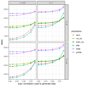
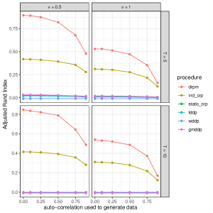
Figure 4: Results from simulation study with data that contains AR(1)-type temporal correlation. The left plot corresponds to results for the model fit metric WAIC and the right plot displays results associated with ARI.

4 Application

In this section we apply our method to a real-world data set coming from the field of environmental science. A second application in education is provided in Section LABEL:SIMCE.application of the online supplementary material. As mentioned previously, once a partition model is specified, there is quite a bit of flexibility regarding how (or if) temporal dependence is incorporated in other parts of a hierarchical model. To illustrate this, we incorporate temporal dependence in three places of the hierarchical model we construct.

As part of preliminary exploratory data analysis (not shown), we examined serial dependence for each experimental unit (monitoring station), and concluded that they all exhibited a particular type of temporal dependence. Because of this, we introduce a unit-specific temporal dependence parameter $|\eta_{1i}|\leq 1$ and model observations from a single unit over time ($Y_{1i},\ldots,Y_{iT}$) with an AR(1) structure. In addition, motivated by a desire for parsimony, we employed a Laplace prior for $\eta_{1i}$. Finally, to permit the temporal dependence in the partition model to propagate through the hierarchical model, we assume an AR(1) structure for the $\theta_{t}$’s. The full hierarchical model is detailed in (13).

$$Y_{it}\mid Y_{it-1},\bm{\mu}^{\star}_{t},\bm{\sigma}^{2\star}_{t},\bm{\eta},\bm{c}_{t} \stackrel{{\scriptstyle ind}}{{\sim}}N(\mu^{\star}_{c_{it}t}+\eta_{1i}Y_{it-1},\sigma_{c_{it}t}^{2\star}(1-\eta_{1i}^{2})),$$ (13)

$$Y_{i1} \stackrel{{\scriptstyle ind}}{{\sim}}N(\mu^{\star}_{c_{i1}1},\sigma_{c_{i1}1}^{2\star}),$$

$$\xi_{i}=\mbox{Logit}(0.5(\eta_{1i}+1)) \stackrel{{\scriptstyle iid}}{{\sim}}Laplace(a,b),$$

$$(\mu_{jt}^{\star},\sigma^{\star}_{jt}) \stackrel{{\scriptstyle ind}}{{\sim}}N(\theta_{t},\tau_{t}^{2})\times UN(0,A_{\sigma}),$$

$$\theta_{t}\mid\theta_{t-1} \stackrel{{\scriptstyle ind}}{{\sim}}N((1-\phi_{1})\phi_{0}+\phi_{1}\theta_{t-1},\lambda^{2}(1-\phi_{1}^{2})),$$

$$(\theta_{1},\tau_{t}) \sim N(\phi_{0},\lambda^{2})\times UN(0,A_{\tau}),$$

$$(\phi_{0},\phi_{1},\lambda) \sim N(m_{0},s_{0}^{2})\times UN(-1,1)\times UN(0,A_{\lambda}),$$

$$\{\bm{c}_{t},\ldots,\bm{c}_{T}\} \sim tRPM(\bm{\alpha},M),\ \mbox{with $\alpha_{t}\stackrel{{\scriptstyle iid}}{{\sim}}Beta(a_{\alpha},b_{\alpha})$},$$

where all Roman letters correspond to parameters that are user supplied. There are a number of special cases embedded in our hierarchical model. For example, $\eta_{i1}=0$ for all $i$ results in conditionally independent observations. Further, $\phi_{1}=0$ results in independent atoms and $\alpha_{t}=0$ for all $t$ in independent partitions over time. The model (7) used in the simulation studies is a special case of (13), obtained by setting $\phi_{1}=0$ and $\eta_{i1}=0$ for all $i$.

4.1 Rural Background PM₁₀ Data Application

The rural background PM₁₀ data is taken from the European air quality database. These data are comprised of the daily measurements of particulate matter with a diameter less than 10 $\mu$m from rural background stations in Germany and are publicly available in the gstat package (Gräler et al. 2016) found on CRAN in R (R Core Team 2020). We focus on average monthly PM₁₀ measures from the year 2005 ( i.e., $T=12$). Of the 69 stations, 9 were removed because of missing values.

We fit the hierarchical model (13) to these data and consider all the possible special cases (i.e., $\eta_{1i}=0$ or not, $\phi_{1}=0$ or not, $\alpha_{t}=0$ or not). This resulted in 8 total models that were fit by collecting 1,000 MCMC iterates after discarding the first 10,000 as burn-in and thinning by 40 (i.e., 50,000 total MCMC samples were collected). Running the algorithm for 50,000 samples on a laptop with 16GB of RAM took between 1 and 2.5 minutes. We use the following prior values: $A_{\sigma}=10$, $A_{\tau}=A_{\lambda}=5$, $m_{0}=0$, $s^{2}=100$, $a=0$, $b=1$, and $a_{\alpha}=b_{\alpha}=2$. The prior for $\alpha_{t}$ was specified to encourage $\alpha$ from approaching 1. The WAIC and log pseudo marginal likelihood (LPML) for each model are presented in Table 3. To improve the computational stability of the LPML, for each model fit, the MCMC iterates that correspond to 0.5% of the smallest likelihood values were not included in the calculation of LPML.

First we note that among all the model fits, employing a variant of $tRPM(\bm{\alpha},M)$ (i.e., rows with “Yes” in the “In Partition” column) improves model fit. The best performing model in terms of WAIC includes temporal dependence in the partition model only, while that for LPML includes temporal dependence in the partition model and in the likelihood.

Now focusing on partition inference, we provide Figure 5. This figure displays the lagged ARI values for each of the 8 models. Notice that when partitions are modeled independently (first or third rows of Figure 5) then partitions evolve over time quite erratically in the sense that the cluster configuration can change dramatically from one time point to the next. However, when employing $tRPM(\bm{\alpha},M)$ (second row of Figure 5) the partitions seemed to evolve much more “smoothly” as there is less drastic changes in cluster configuration. In fact the model that produces the best model fit metrics (right most plot of second row) seems to produce partitions that change quite gently over time as desired.

Table 3: PM₁₀ data: Results of model fitting. The bold font identifies best model fits in terms of LPML and WAIC. Higher values for LPML indicate better fit while lower values for WAIC indicate better fit.

Temporal Dependence In
Likelihood ($\eta_{1i}$)	Atoms ($\phi_{1}$)	Partition ($\alpha_{t}$)	LPML	WAIC
No	No	No	-1814	3683
No	No	Yes	-1656	3031
No	Yes	No	-1752	3539
No	Yes	Yes	-1644	3271
Yes	No	No	-1704	3554
Yes	No	Yes	-1578	3186
Yes	Yes	No	-1706	3544
Yes	Yes	Yes	-1586	3153

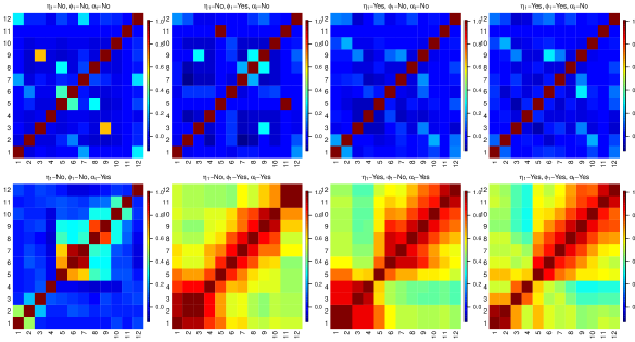
Figure 5: PM₁₀ data. Each figure is a summary of the lagged $ARI$ values corresponding to the 8 models in Table 3. At each time point the partition was estimated using the salso function in the salso R package (Dahl et al. 2020) based on binder loss.

Finally, we provide Figure 6 as a means to visualize how estimated partitions based on our joint partition model evolve over time relative to modeling partitions with an $iid$ model. Each plot in Figure 6 displays the estimated partition at each time point. Each color represents a cluster and each number corresponds to a specific measuring station. The plots illustrate the sequential nature of cluster forming with the first cluster always containing the first measuring station, the next cluster is formed by the first station not included in the first cluster and so on. The plots in the right column correspond to using $tRPM(\bm{\alpha},M)$ to jointly model partitions while those on the right employ $\rho_{t}\stackrel{{\scriptstyle iid}}{{\sim}}CRP(M)$. It is evident from Figure 6 that from one time point to the next that partitions based on our construction evolve much more gently over time. This more closely mimics how PM₁₀ measurements would evolve as a function of time compared to the iid model.

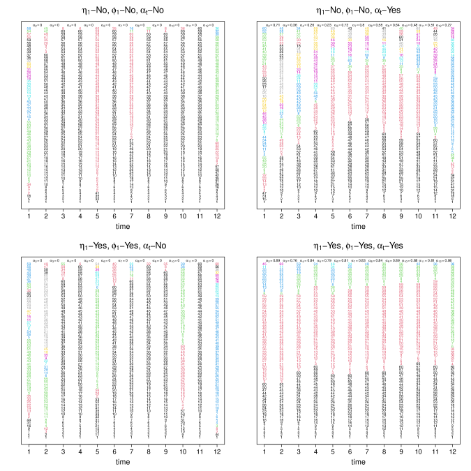
Figure 6: Each plot displays the estimated partition at each time point. Plots in the left column are based on $\rho_{t}\stackrel{{\scriptstyle iid}}{{\sim}}CRP(M)$ while those in the right column are based on $(\rho_{1},\ldots,\rho_{T})\sim tRPM(\bm{\alpha},M)$. Clusters are highlighted by color and each number corresponds to a specific monitoring station.

4.2 Extensions to the Joint Partition Model

Based on our generic joint model construction, it is straightforward to incorporate other information in the partition model such as covariates. For example, in the data application of 4.1 each monitoring station’s spatial coordinates were recorded. Incorporating spatial dependence in our analysis of the PM₁₀ data can be easily accommodated via the EPPF in our construction. This would result in spatially informed clusters that evolve over time. If the spatially referenced EPPF preserves sample size consistency, then Proposition 1 still holds. One such EPPF is part of the spatial product partition model (sPPM) class developed in Page and Quintana (2016). To illustrate the ease of incorporating space in our model construction, here we model the PM₁₀ data using model (13) but rather than use the $tRPM(\bm{\alpha},M)$ to model the sequence of partitions, we use a version of our dependent partition model that employs the sPPM.

In order to introduce the sPPM, let $\bm{s}_{i}$ denote the spatial coordinates of the $i$th item (note that these coordinates do not change over time) and let $\bm{s}^{\star}_{jt}$ be the subset of spatial coordinates that belong to the $j$th cluster at time $t$. Then we express the EPPF of the $t$th partition with the following product form

$$\text{Pr}(\rho_{t}\mid\nu_{0},M)\propto\prod_{j=1}^{k_{t}}c(S_{jt}\mid M)g(\bm{s}^{\star}_{jt}\mid\nu_{0}).$$ (14)

Here $c(\cdot\mid M)\geq 0$ is called the cohesion and is a set function that produces cluster weights a priori. We consider the cohesion $c(S_{jt}\mid M)=M\times(|S_{jt}|-1)!$ as it has connections with the CRP making this version of the sPPM a type of spatially re-weighted CRP. The similarity function $g(\cdot\mid\nu_{0})$ is a set function parametrized by $\nu_{0}$ that measures the compactness of the spatial coordinates in $\bm{s}^{\star}_{jt}$ producing higher values if the spatial coordinates in $\bm{s}^{\star}_{jt}$ are close to each other. Not all similarity functions preserve sample size consistency so to ensure this, after standardizing spatial locations, we employ

$$g(\bm{s}^{\star}_{jt}\mid\nu_{0})=\int\prod_{i\in S_{jt}}N(\bm{s}_{i}\mid\bm{m},\bm{V})NIW(\bm{m},\bm{V}\mid\bm{0},1,\nu_{0},\bm{I})\,d\bm{m}\,d\bm{V},$$ (15)

where $N(\cdot\mid\bm{m},\bm{V})$ denotes a bivariate normal density and $NIW(\cdot,\cdot\mid\bm{0},1,\nu_{0},\bm{I})$ a normal-inverse-Wishart density with mean $\bm{0}$, scale equal to 1, inverse scale matrix equal to $\bm{I}$, and $\nu_{0}$ being the user-supplied degrees of freedom. Note that larger values of $\nu_{0}$ increase spatial influence on partition probabilities. For more details on why this formulation preserves sample size consistency, see Müller et al. (2011) and Quintana et al. (2018). For more information regarding the impact of $\nu_{0}$ on product form of the partition model, see Page and Quintana (2016, 2018). We will use $stRPM(\bm{\alpha},\nu_{0},M)$ to denote our spatio-temporal random partition model (6) parameterized by $\alpha_{1},\ldots,\alpha_{T}$ and EPPF detailed in (14) and (15).

As in the previous section, we fit model (13) to the PM₁₀ data but replacing $tRPM(\bm{\alpha},M)$ with the $stRPM(\bm{\alpha},\nu_{0},M)$. Also as before, we consider all the possible special cases of the model (i.e., $\eta_{1i}=0$ or not, $\phi_{1}=0$ or not, $\alpha_{t}=0$ or not). This resulted in 8 total models that were fit by collecting 1,000 MCMC iterates after discarding the first 10,000 as burn-in and thinning by 40. Fitting the eight models based on the $stRPM(\bm{\alpha},\nu_{0},M)$ took between 20 and 57 minutes. The prior values employed were the same as before with the addition of setting $\nu_{0}=5$ which places in the partition prior moderate weight on spatial locations.

Incorporating space in the partition model seems to provide benefit in terms of model fit as the LPML and WAIC values associated with the model that includes space in the partition model and temporal dependence in all levels of the model fits best in terms of LPML with -1487 compared to -1586 listed in Table 3 and temporal dependence in partition and atoms fits best with regards to WAIC with 3140 compared to 3271 listed in Table 3. Additionally, Figure 7 displays the lagged ARI values for the 8 models that include space. As in Figure 5 when there is no temporal dependence in the partition model, then the estimated partitions exhibit no temporal dependence. However, when time and space are included then there is clear dependence between partitions as a function of time. Further, the dependence between partitions seems to decay faster with space and time included in the partition model compared to just time.

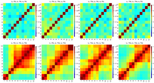
Figure 7: PM₁₀ data. Each figure is a summary of the lagged $ARI$ values corresponding to the 8 models that are detailed in Table 3 except that space is also included in the dependent random partition model. At each time point the partition was estimated using the salso function in the salso R package (Dahl et al. 2020) based on binder loss.

Finally, we provide Figure 8 which displays the estimated spatially referenced partitions at each time point based on the model that achieved the best fit (space in the partition model and temporal dependence in all levels of the model). The size of each point in the figure is proportional to the PM₁₀ measured at the particular station and each depicts a cluster. To make connections with Figure 6 each monitoring station is labeled with the same number as before. Notice that there are clear similarities from one time point to the next for most months. That said, there are two time periods for which changes in the PM₁₀ are more drastic relative to the previous time period (e.g., August to September). In these months the estimated $\alpha_{t}$ is quite a bit smaller and as a result, the estimated partitions are more different.

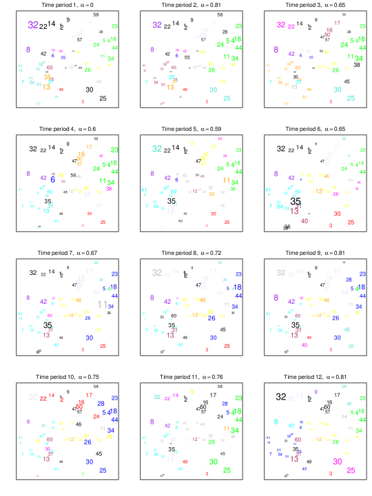
Figure 8: PM₁₀ data. Graphical display for spatially-referenced estimated partitions for each time point based on the model that produced best fit (space in the partition model and temporal dependence in all levels of the model). The size of a point is proportional to the PM₁₀ measured at that station. Clusters are identified by color. Each monitoring station is labeled by the same numbers as in Figure 6. At each time point the partition was estimated using the salso function in the salso R package (Dahl et al. 2020) based on binder loss.

5 Conclusions

We developed a joint probability model for a sequence of partitions that explicitly considers temporal dependence among the partitions. Further, we showed that our methodology is capable of accommodating partitions that evolve slowly over time in that the adjusted Rand index between estimated partitions decays as the lag in time increases. We also showed that if partitions are indeed independent over time, then employing our joint partition prior regardless results in a minimal cost in terms of model fit.

The predictive nature of the temporal prior on a sequence of random partitions we have presented has a first-order Markovian structure. Various extensions can be considered, such as adding higher order dependence across time or dependence in baseline covariates. All of these cases would build on our constructive definition, as extra refinements of the basic idea of carrying smooth transitions on time (or time and space). Lastly, the Markovian structure could be exploited to carry out predictive inference as well.

SUPPLEMENTARY MATERIAL

Supplementary Material:

Online supplementary material file that contains proofs of propositions, computation details, additional simulation, and application results.

R-package:

The R-package drpm contains the function drpm that fits all models described in the article.

References

- Antoniano-Villalobos and Walker (2016) Antoniano-Villalobos, I. and Walker, S. G. (2016), “A nonparametric model for stationary time series,” J. Time Series Anal., 37, 126–142.
- Binder (1978) Binder, D. A. (1978), “Bayesian Cluster Analysis,” Biometrika, 65, 31–38.
- Caron et al. (2007) Caron, F., Davy, M., and Doucet, A. (2007), “Generalized Polya Urn for Time-varying Dirichlet Process Mixtures,” in Proceedings of the Twenty-Third Conference on Uncertainty in Artificial Intelligence, UAI’07, Arlington, Virginia, United States: AUAI Press, URL http://dl.acm.org/citation.cfm?id=3020488.3020493.
- Caron et al. (2017) Caron, F., Neiswanger, W., Wood, F., Doucet, A., and Davy, M. (2017), “Generalized Pólya Urn for Time-Varying Pitman-Yor Processes,” Journal of Machine Learning Research, 18, 1–32, URL http://jmlr.org/papers/v18/10-231.html.
- Corradin et al. (2020) Corradin, R., Canale, A., and Nipoti, B. (2020), BNPmix: Bayesian Nonparametric Mixture Models, URL https://CRAN.R-project.org/package=BNPmix. R package version 0.2.6.
- Corradin et al. (2021) — (2021), “BNPmix: an R package for Bayesian nonparametric modelling via Pitman-Yor mixtures,” Journal of Statistical Software, to appear.
- Dahl et al. (2020) Dahl, D. B., Johnson, D. J., and Müller, P. (2020), salso: Search Algorithms and Loss Functions for Bayesian Clustering, URL https://CRAN.R-project.org/package=salso. R package version 0.2.5.
- De Blasi et al. (2015) De Blasi, P., Favaro, S., Lijoi, A., Mena, R. H., Prünster, I., and Ruggiero, M. (2015), “Are Gibbs-Type Priors the Most Natural Generalization of the Dirichlet Process?” IEEE Transactions on Pattern Analysis and Machine Intelligence, 37, 212–229.
- De Iorio et al. (2019) De Iorio, M., Favaro, S., Guglielmi, A., and Ye, L. (2019), “Bayesian nonparametric temporal dynamic clustering via autoregressive Dirichlet priors,” ArXiv:1910.10443.
- DeYoreo and Kottas (2018) DeYoreo, M. and Kottas, A. (2018), “Modeling for dynamic ordinal regression relationships: an application to estimating maturity of rockfish in California,” Journal of the American Statistical Association, 113, 68–80, URL https://doi.org/10.1080/01621459.2017.1328357.
- Gelman et al. (2014) Gelman, A., Hwang, J., and Vehtari, A. (2014), “Understanding predictive information criteria for Bayesian models,” Statistics and Computing, 24, 997–1016.
- Gräler et al. (2016) Gräler, B., Pebesma, E., and Heuvelink, G. (2016), “Spatio-Temporal Interpolation using gstat,” The R Journal, 8, 204–218, URL https://journal.r-project.org/archive/2016-1/na-pebesma-heuvelink.pdf.
- Gutiérrez et al. (2016) Gutiérrez, L., Mena, R. H., and Ruggiero, M. (2016), “A time dependent Bayesian nonparametric model for air quality analysis,” Computational Statistics & Data Analysis, 95, 161 – 175.
- Hubert and Arabie (1985) Hubert, L. and Arabie, P. (1985), “Comparing Partitions,” Journal of Classification, 2, 193–218.
- Jo et al. (2017) Jo, S., Lee, J., Müller, P., Quintana, F. A., and Trippa, L. (2017), “Dependent Species Sampling Models for Spatial Density Estimation,” Bayesian Analysis, 12, 379–406, URL https://doi.org/10.1214/16-BA1006.
- Kalli and Griffin (2018) Kalli, M. and Griffin, J. E. (2018), “Bayesian nonparametric vector autoregressive models,” Journal of Econometrics, 203, 267–282.
- Müller et al. (2011) Müller, P., Quintana, F., and Rosner, G. L. (2011), “A Product Partition Model With Regression on Covariates,” Journal of Computational and Graphical Statistics, 20, 260–277.
- Müller et al. (2015) Müller, P., Quintana, F. A., Jara, A., and Hanson, T. (Editors) (2015), Bayesian Nonparametric Data Analysis, Switzerland: Springer International Publishing, 1 edition.
- Neal (2000) Neal, R. M. (2000), “Markov Chain Sampling Methods for Dirichlet Process Mixture Models,” Journal of Computational and Graphical Statistics, 9, 249–265.
- Nieto-Barajas et al. (2012) Nieto-Barajas, L. E., Müller, P., Ji, Y., Lu, Y., and Mills, G. B. (2012), “A Time-Series DDP for Functional Proteomics Profiles,” Biometrics, 68, 859–868.
- Page and Quintana (2016) Page, G. L. and Quintana, F. A. (2016), “Spatial Product Partition Models,” Bayesian Analysis, 11, 265–298.
- Page and Quintana (2018) — (2018), “Calibrating Covariate Informed Product Partition Models,” Statistics and Computing, 28, 1009–1031, URL https://doi.org/10.1007/s11222-017-9777-z.
- Quintana et al. (2018) Quintana, F. A., Loschi, R. H., and Page, G. L. (2018), Bayesian Product Partition Models, Wiley StatsRef: Statistics Reference Online, 1–15, URL https://onlinelibrary.wiley.com/doi/abs/10.1002/9781118445112.stat08123.
- Quintana et al. (2020) Quintana, F. A., Müller, P., Jara, A., and MacEachern, S. N. (2020), “The Dependent Dirichlet Process and Related Models,” ArXiv:2007.06129v1.
- R Core Team (2020) R Core Team (2020), R: A Language and Environment for Statistical Computing, R Foundation for Statistical Computing, Vienna, Austria, URL https://www.R-project.org/.
- Rand (1971) Rand, W. M. (1971), “Objective Criteria for the Evaluation of Clustering Methods,” Journal of the American Statistical Association, 66, 846–850.
- Sethuraman (1994) Sethuraman, J. (1994), “A constructive definition of Dirichlet priors,” Statistica Sinica, 4, 639–650.
- Wade et al. (2014) Wade, S., Walker, S. G., and Petrone, S. (2014), “A Predictive Study of Dirichlet Process Mixture Models for Curve Fitting,” Scandinavian Journal of Statistics, 41, 580–605.
- Zanini et al. (2019) Zanini, C. T. P., Müller, P., Ji, Y., and Quintana, F. A. (2019), “A Bayesian Random Partition Model for Sequential Refinement and Coagulation,” Biometrics, 75, 988–999.