Evaluation of the spectrum of a quantum system using machine learning based on incomplete information about the wavefunctions.

Abstract

We propose an effective approach to rapid estimation of the energy spectrum of quantum systems with the use of machine learning (ML) algorithm. In the ML approach (back propagation), the wavefunction data known from experiments is interpreted as the attributes class (input data), while the spectrum of quantum numbers establishes the label class (output data). To evaluate this approach, we employ two exactly solvable models with the random modulated wavefunction amplitude. The random factor allows modeling the incompleteness of information about the state of quantum system. The trial wave functions fed into the neural network, with the goal of making prediction about the spectrum of quantum numbers. We found that in such configuration, the training process occurs with rapid convergence if the number of analyzed quantum states is not too large. The two qubits entanglement is studied as well. The accuracy of the test prediction (after training) reached 98 percent. Considered ML approach opens up important perspectives to plane the quantum measurements and optimal monitoring of complex quantum objects.

Introduction. The applications of intelligent machines in various context of scientific research recently become an area of active investigations PNAS:2018 ; Linglong:2018 ; Lunden:2011 ; JAP-Urban:2019 ; JAP-Damir:2018 ; Laura:2018 ; Juan:2017 ; Salvail:2013 ; PNAS:2018 ; Vogel:1989 ; Smithey:1993 ; Breitenbach:1997 ; White:1999 ; Hofheinz:2009 ; Steinbrecher:2019 . One of the important perspective directions of quantum physics is the measurement of wave functions and the energy spectrum of quantum objects. At present, the wavefunction is determined using the tomographic methods Vogel:1989 -Hofheinz:2009 , which evaluate the wavefunction that is most compatible with a diverse set of measurements. The indirectness of these methods compounds the problem of direct determining the wavefunction. To overcome this problem, it was shown Lunden:2011 that the photon wavefunction can be measured directly by sequentially measuring two additional system variables. As result, the components of the wavefunction appear directly on the measuring apparatus. The alternative approach can be used to determine the polarization quantum state Salvail:2013 . In contrast to various works motivated by physically oriented approaches to artificial intelligence, there are much fewer practical studies estimating the energy spectrum (spectral numbers) for a quantum system based on incomplete information about the wavefunction with the use of the machine learning (ML) approaches. The information on the quantum object structure normally is obtained as the result of measurements of the wavefunction in series of experiments. By the measurements we mean the definition values of wavefunction at a number of spatial points $x_{j}$, see Ref.Lunden:2011 Fig.2(a). According to the Heisenberg uncertainty principle, in quantum theory, an exact measurement of position $X$ violates the wavefunction of the particle and forces the subsequent measurement of momentum $P$ to become random. To include such a factor into consideration in the machine learning (ML), we model uncertainty as a random modulation of the measured amplitude of the wavefunction. Thus an incomplete wavefunction can be written as $\widetilde{\Psi}_{k}(x_{i}|n_{j})=\gamma\Psi(x_{i}|n_{j})$, where $k$ is the number of measurement, $n_{j}$ is a spectral number for $j-$state, and $\gamma$ is random valued variable. However, such ML way has not been realized hitherto. The purpose of this paper is to present an effective approach to solution of this problem. Herein, we create a neural network (NN) and investigate the use of the controlled ML method to generate predictions for the energy spectrum based on incomplete information on the wavefunction of a quantum system. To evaluate this approach, we employ two exactly solvable models with different structure of the energy spectrum and the different field polarization.

Machine learning. To apply the supervised machine learning (ML) technique we first have to construct the dataset $R$ to train the neural network (NN). Our approach is based on the following strategy. (i) We calculate the wavefunctions from the solution of the Schrödinger equation (SE) $H\Psi_{n}=E_{n}\Psi_{n}$, with $\Psi_{n}(x_{i})=\Psi_{ni}$ in spatial points $x_{i}$ , $i=1..,I$, where $I$ is total number of points in which the value of the wavefunction is measured. (Similar structure of $\Psi_{n}$ measurements was used in the experiment Lunden:2011 ). (ii) For every spectral number $n_{j},j=1,2,...J$ ( $J$ is the number of states in energy spectrum) we prepare the matrices $R_{j}$ of sizes $I\times K$ constructed in following way. We multiply the wavefunctions $\Psi_{ni}$ by random-valuated factor $\gamma$ (uniform noise) that produces a set of perturbed wavefunctions $\Psi(x_{i}|n_{j})\rightarrow\widetilde{\Psi}_{k}(x_{i}|n_{j})\equiv\gamma\Psi(x_{i}|n_{j})$ , where $k=1...K$, $k$ is number of the experiment and the variable $K$ (total number of experiments) is arbitrary parameter, normally we used $K\leq 100$. Here the random factor $\gamma$ simulates the uncertainness of the wavefunction amplitude in a real experiment. In our study $\gamma$ is uniform quasi-random variable with large period of repetition that is recalculated at every computing steps. In last column $R_{j}$ it is inserted the spectral number $n_{j}$ corresponding to the energy spectrum of $\Psi_{n}$. (iii) Lastly, we construct the large matrix $R=R_{1}\oplus$ $R_{2}\oplus$ … $R_{J}$ that serves as the input dataset for our NN. Such total matrix $R=R(\widetilde{\Psi}_{k}(x_{i}|n_{j}))$ has the following structure

$$R=\left\{\begin{array}[c]{cccccc}\widetilde{\Psi}_{1}(x_{1}|n_{1})&\widetilde{\Psi}_{2}(x_{2}|n_{1})&...&...&\widetilde{\Psi}_{K}(x_{I}|n_{1})&n_{1}\\ \widetilde{\Psi}_{K+1}(x_{1}|n_{1})&\widetilde{\Psi}_{K+2}(x_{2}|n_{1})&...&...&\widetilde{\Psi}_{2K}(x_{I}|n_{1})&n_{1}\\ ...&...&...&...&...&...\\ \widetilde{\Psi}_{1}(x_{1}|n_{2})&\widetilde{\Psi}_{2}(x_{2}|n_{2})&...&...&\widetilde{\Psi}_{K}(x_{I}|n_{2})&n_{2}\\ ...&...&...&...&...&...\\ \widetilde{\Psi}_{1}(x_{1}|n_{3})&...&...&...&...&n_{3}\end{array}\right\}$$ (1)

It is notably, (a) that the randomly perturbed wavefunctions $\widetilde{\Psi}_{k}(x_{i}|n_{j})$ in Eq.(1) already are not the exact solutions of the Schrödinger equation, however, they still relay to the spectral spectral numbers $n_{j}$, and (b) since at training all the rows in the dataset $R$ are randomly interchanged, the initial order of rows in $R$ is not important. In the following Section we will use $R$ matrix as the input dataset, where in accordance to ML terminology the values $\widetilde{\Psi}_{k}(x_{i}|n_{j})$ are defined as the attributes (features) class, while the spectrum $n_{j}$ is defined as the label class (categorical values Schmidhuber:2015 ; Haykin:2009 ; Kelleher:2015 ).

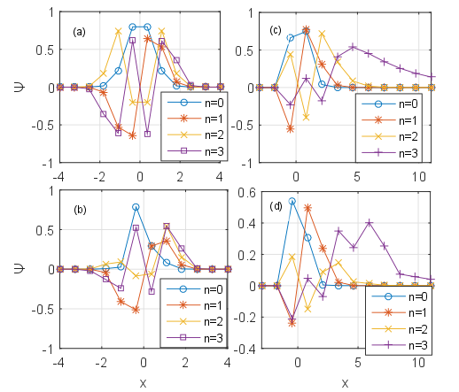
Figure 1: (Color on line.) (a) Spatial structure of the unperturbed wavefunctions $\Psi_{n,j}$ (calculated for $12$ nodes) of the linear oscillator for spectral numbers $n_{j}=0,1,2,3$ and $V_{0}=3$; (b) The same as in (a) but for wavefunctions $\widetilde{\Psi}_{ni}$ randomly perturbed by uniform random noise with amplitude $A=1$; (c) Spatial structure of the unperturbed wavefunctions $\Psi_{n,j}$ (calculated for $12$ nodes) of the no-symmetric Morse potential for $V_{0}=7,\alpha=1$. In this case the condition $\sqrt{2V_{0}}/\alpha>n+\frac{1}{2}$ leads that only 4 discrete states $n_{j}=0,1,2,3$ are allowed. (d) The same as in (c) but for randomly perturbed wavefunctions $\widetilde{\Psi}_{ni}$ by the uniform random noise.

Neural network. We construct the NN and apply the ML technique to generate predictions of spectral numbers $n_{j}$ that allow defining the energy spectrum of the studied quantum system. For our ML studies we create a supervised NN by standard technique Kelleher:2015 with the use of matrix $R$ from Eq.(1). We use the back-propagation algorithm, which is one of the common algorithms applied to train NN. In this paper, as a basic NN we used the scheme from Ref.McCaffey:2015 , which, however, has been refined and considerably expanded to reach our purpose: apply the numerical perturbed wavefunctions $\widetilde{\Psi}_{nj}$ to predict the spectral numbers $n_{j}$. The values of the outputs $n_{j}$ are determined by the input values $\widetilde{\Psi}_{nj}$, by the NN parameters: number of hidden processing nodes that allow generating a set of weights and bias values. We created the fully connected NN with $I_{L}$ inputs, $H_{L}$ hidden nodes and $O_{L}$ outputs that has $I_{L}H_{L}+H_{L}+H_{L}O_{L}+O_{L}$ weights and biases. The next step is training of NN to calculate the values for the weights $W_{L}$ and biases $B_{L}$ such that, for our set of training data $R$ (with known input $\widetilde{\Psi}_{k}(x_{i}|n_{j})$ and output $n_{j}$ values) the computed outputs of the NN has to closely match the known outputs. In our simulation, the program splits the input dataset $R$ randomly into two parts: training set and test set. The training set (80%) is used to create the neural network model, while the test set (20%) is used to estimate the accuracy of predictions. Besides of the number of hidden nodes $H_{L}$ the following additional back-propagation parameters are used in NN: the maximum number of training iterations $T_{\max}$, the learning rate $L_{R}$ (that allows to controls the steepest descent process), and the momentum rate $M_{R}$. The momentum rate helps to prevent the training from the getting stuck with local, non-optimal weight values and also prevents the oscillation where training never converges to stable values. In realistic approach all the mentioned parameters are determined at calculations by the trial and error. Also the program calculates the mean squared error that allows to control the over-fitting at re-trainingKelleher:2015 .

Exactly solvable models. To evaluate the applicability of the ML approach, we employ two exactly solvable models with the random modulated wave functions. To do that we consider the Schrödinger equation (SE) solutions (to seek for simplification we use here the atomic units allowing to set $m=1$ and $\hbar=1$)

$$(1/2)d^{2}\Psi_{n}/dx^{2}+[E-V(x)]\Psi_{n}=0.$$ (2)

The solutions of Eq.(2) yield us the wavefunctions $\Psi(x_{i}|n_{j})$ allowing to create the perturbed wavefunctions $\widetilde{\Psi}_{k}(x_{i}|n_{j})=\gamma\Psi(x_{i}|n_{j})$ that are used in the input dataset $R$ in Eq.(1). Two well-known models: linear oscillator and Morse potentialLandauQM are used here.

Linear oscillator. In this case in Eq.(2) $V(x)=V_{0}x^{2}$ and the solution reads $\Psi_{n}=(\frac{\omega}{\pi})^{1/4}\exp(-\frac{\omega}{2}x^{2})H_{n}(x\sqrt{\frac{\omega}{\pi}})$, where $\omega=\sqrt{2V_{0}}$, $H_{n}(\xi)$ are the Hermit polynomials, and $E_{n}=(n+\frac{1}{2})\omega$ is the energy for different spectral numbers $n=0,...J<\infty$  LandauQM . Fig.1 (a) displays the initial wavefunctions with $V_{0}=3,$ $I=12$ (number of measurements points) and $J=4$ for states with $n=0,1,2,3$, while Fig.1(b) exhibits the randomly perturbed functions $\widetilde{\Psi}_{\gamma}(x_{i}|n_{j})$, shown in Fig.1(a), but modulated by random noise $\gamma$  (uniformly distributed random numbers in $[0,...,1]$).

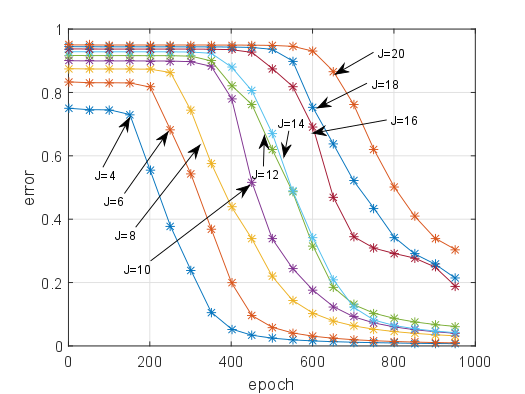
Figure 2: (Color on line) The value of the error training $\varepsilon_{T}$ as function of the epoch numbers at training the linear oscillator dataset (matrix $R$ of the perturbed wavefunctions $\widetilde{\Psi}_{\gamma}(x_{i}|n_{j})$) for different spectral numbers in the spectrum $J$ from $J=4$ (with $n=0,1,2,3$) to $J=20$ (with $n=0,1,2,...,19$). We observe that the larger number of spectrum $J$ the larger number of epochs at training it is necessary to reach small errors.

The random factor $\gamma$ is recalculated at every calculation step, thus the spatial structure of $\widetilde{\Psi}_{k}(x_{i}|n_{j})$ changes significantly for every recalculating circle and it is different for every rows (experiment $k$) in Eq.(1). The trial wavefunctions $\widetilde{\Psi}_{k}(x_{i}|n_{j})$ fed into NN, with the goal of making prediction about the spectrum of quantum numbers $n_{j}$.  The parameters of constructed NN may vary to improve the quality of predictions, initially we used $I_{L}=I=12$ inputs (features), $J=O_{L}=4$ (outputs), and $H_{L}=5$ hidden layers, see Fig.1 (a),(b). The appropriate choice of the learning (back-propagation) parameters are assigned for the training $T_{max}=1000$, $R_{L}=0.005$, $M_{L}=1$ , which are found to optimize the efficiency of the NN model. To monitor the dynamics of training we calculated the mean squared error $\varepsilon_{T}=N^{-1}\sum_{i=1}^{N}(t_{i}-y_{i})^{2}$ that indicates a difference between the predicted value $t_{i}$ and the true value $y_{i}$.

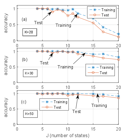
Figure 3: (Color on line.) The accuracy of training $a_{tr}$ and accuracy of the test $a_{ts}$ for the spectral numbers $n_{j}$ predictions as function of the maximal number of studied quantum states $J$ at different number of experiments $K$, (a) $K=20$, (b) $K=30$, (c) $K=50$. We observe that the accuracy $a_{ts}$ strongly depends on the quantity of experiments $K$. For small $n_{j}<6$ the accuracy is high $a_{ts}\simeq 95\%$ already at $K=20$, but for large $n_{j}>10$ the accuracy $a_{ts}$ falls. One can say the larger number of spectrum $J$ the larger number of experiments $K$ is necessary to reach the desired accuracy.

Fig. 2 shows the evolution of $\varepsilon_{T}$ as function of the epoch numbers for the linear oscillator case. From Fig. 2 one can see quite fast convergence of the training (for not large spectral numbers $n$) that leads to small training errors $\varepsilon_{T}\leq 10^{-2}$ already for $500$ epochs. The convergence of the training shown in Fig. 2 for not large $n<14$ brings the test prediction accuracy for the linear oscillator model $a_{Ts}=$ $N_{c}/N$ about $\sim 97\%$ and better (here $N_{c}$ is number of correct predictions, $N$ is total number of predictions). However the prediction accuracy for large $n$ may be significantly improved at the use of larger number of the epoch training $T_{max}>2000$. Fig. 3 exhibits the accuracy of training $a_{tr}$ and the accuracy of test $a_{ts}$ for the spectral numbers $n_{j}$ predictions as function of the maximal number of studied quantum states $J$ at different number of experiments $K$, Fig. 3 (a) $K=20$, (b) $K=30$, (c) $K=50$. We observe from Fig. 3 that the accuracy $a_{ts}$ strongly depends on the quantity of experiments $K$. For small $n_{j}<6$ the accuracy is high $a_{ts}\simeq 95\%$ already at $K=20$, but for large $n_{j}>10$ the accuracy $a_{ts}$ decreases. One can say the larger number of spectrum J the larger number of experiments is necessary to reach the desired accuracy.

Morse potential. In this case in Eq.(2) $V(x)=V_{0}(\exp(-2\alpha x)-2\exp(-\alpha x))$. In this potential case SE reads $\frac{d^{2}\psi}{dx^{2}}+2(E-A(\exp(-2\alpha x)-2\exp(-\alpha x))\psi=0$ with the solution $\psi=\exp(-\xi/2)\xi^{s}w(\xi)$ where $\xi=\frac{2\sqrt{2A}}{\alpha}\exp(-\alpha x)$ and $w$ can be expressed as a hypergeometric polynomial $w(\xi)=F(-n,2s+1,\xi)$. Here $s=\frac{2\sqrt{-2E}}{\alpha},n=\frac{\sqrt{2A}}{\alpha}-(s+\frac{1}{2})$. The latter allows the finite energy spectrum $E_{n}=A[1-\frac{\alpha}{\sqrt{2A}}(n+\frac{1}{2})]^{2},n=0,1..<n_{max}$. Therefore it has to be $\frac{\sqrt{2V_{0}}}{\alpha}>n+\frac{1}{2}$, so there is not discrete spectrum if $\frac{\sqrt{2A}}{\alpha}<\frac{1}{2}$  LandauQM . Fig.1(c) exhibits the spatial structure of the unperturbed wavefunctions $\Psi_{n,j}$ (calculated for $12$ nodes) of the no-symmetric Morse potential for $V_{0}=7,\alpha=1$. In this case the condition $\sqrt{2V_{0}}/\alpha>n+\frac{1}{2}$ leads that only 4 discrete states $n_{j}=0,1,2,3$ are allowed. Fig.1(d) displays same as in Fig.1(c), but for randomly perturbed wavefunctions by the uniform random noise $\widetilde{\Psi}_{ni}$ .

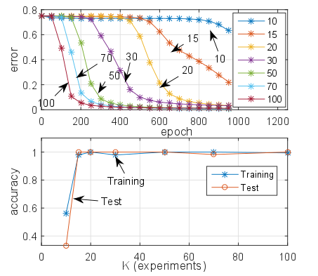
Figure 4: (Color on line) (a) The training error $\varepsilon_{T}$ as function of the epoch number at training the Morse dataset (matrix $R$ of the perturbed wavefunctions) for parameters $V_{0}=7$, $a=1$ (in this case there is energy spectrum with $n=0.1.2.3$). We observe that for ML parameters $R_{L}=0.005$, $M_{L}=1$, $I_{L}=12$, $H_{L}=5$, $O_{L}=4$ the error $\varepsilon_{T}$ becomes small for the epoch iterations $T_{\max}\geq 50$. (b) Training accuracy $a_{Tr}$ and test accuracy $a_{Ts}$ as function of number of experiments $K$.

Fig.4 (a) shows the training error $\varepsilon_{T}$ as function of the epoch number at training of the Morse dataset (matrix $R$ of the perturbed wavefunctions $\widetilde{\Psi}_{\gamma}(x_{i}|n_{j})$) at different $K$ for parameters $V_{0}=7$, $\alpha=1$ (in this case there is only the limited energy spectrum with $n=0.1.2.3$). We observe that for ML parameters $R_{L}=0.005$, $M_{L}=1$, $I_{L}=12$, $H_{L}=5$, $O_{L}=4$ the error $\varepsilon_{T}$ becomes small for the epoch iterations at $T_{\max}\geq 50$. Fig.4 (b) displays the training accuracy $a_{Tr}$ and test accuracy $a_{Ts}$ as function of experiment number $K$. From Fig.4 (b) one can see that accuracy have acceptable values $\geq 95\%$ at quite large value of $K>40.$

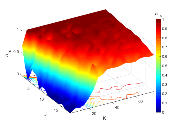
Figure 5: (Color on line) The test accuracy $a_{Ts}$ as function of the spectrum photon numbers $J\in[2..20]$ and the numbers of experiment $K\in[5..100]$ at the spatial points $I=12$ and $1000$ epochs for polarized quantum states (photons) with two different wavelengths $\lambda_{1,2}$.

Advanced quantum model. Now we consider an advanced quantum-mechanical model by adding the linear oscillator with characteristics of the orthogonal polarization state $p_{1},p_{2}$ and the photon wavelength, that is a field state $\arrowvert{p_{1,2}},n,\lambda_{1,2}\rangle$, where $n$ is the numbers of photons radiated with two different wavelengths $\lambda_{1,2}$ (see Chap.14 in Ref. BasdevantQM:2005 ). This allows us referring the experiments Lunden:2011 ; Salvail:2013 , where the wavefunction of photon was directly measured (see Figs.2,3 in Lunden:2011 ). To study such a situation we add one more column (polarization+wavelength) to the features columns in the database $R$, see Eq.(1). Such a feature state $({p_{1,2}},\lambda_{1,2})$ is generated as random numbers in range $\in[1..4]$. Fig.5 shows the test accuracy $a_{Ts}$ as function of the spectrum numbers $J\in[2..20]$ and the experiment numbers $K\in[5..100]$ at the fixed number of spatial points $I=12$ (where $\Psi$ was measured) and $T_{max}=1000$ epochs for polarized quantum states (photons) $\arrowvert{p_{1,2}},n,\lambda_{1,2}\rangle$. One can see from Fig.5 that NN for such the advanced model reaches the acceptable predictions with $a_{Ts}\simeq 1$ only if the number of experiments is large enough $K>20$.

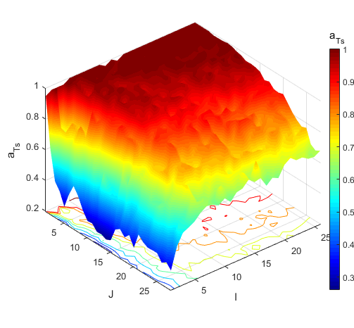
Figure 6: (Color on line) The test accuracy $a_{Ts}$ as function of the spectrum numbers $J\in[2..30]$ and the spatial points $I\in[4..30]$ at fixed number of experiment $K=100$ and $1000$ epochs for photons with wavelength $\lambda_{1,2}$.

Fig.6 shows the test accuracy $a_{Ts}$ as function of the spectrum numbers $J\in[2..30]$ and the spatial points $I\in[4..30]$ at fixed the experiment numbers $K=100$ and $1000$ epochs for polarized photons as in Fig.5. We observe from Fig.6 that the acceptable predictions with $a_{Ts}\simeq 1$ is reached only if a number spatial points $I$ is large enough $I>10$ and the spectrum photon numbers $J<10$.

Discussion. In this paper, we examined the use of NN to predict the energy spectrum (spectral numbers) and the photon entanglement from the measurements of the wave function of a quantum system. A database was built taking into account the number of measurements $J$ and the number of independent experiments on the training $K$. The effectiveness of such a network was demonstrated using two basic different solvable models of the Schrödinger equation. The first model (linear oscillator) has the unlimited energy spectrum, and in the second case (Morse potential) the number of energy levels depends on the amplitude of the potential. To model the uncertainty of wavefunctions, the random amplitude modulation was applied. The values of the wavefunction measurement were required only in a small number of spatial points $I=12$ (Fig.1). Our calculations showed high efficiency of network training when the resulting learning error reached several percent for the number of epochs less than $T_{max}=1000$ (Fig.2). The analysis of the spectral numbers prediction for both models showed that the training efficiency and the test accuracy depend significantly on the maximum quantity of spectral numbers $J$, and on the number of quantum experiments $K$. It was found that the large numbers of the spectrum $J$, the greater the number of epochs in machine learning is necessary to achieve an acceptable learning error. The larger $J$, the more experiments must be performed to achieve a desired accuracy of prediction shown in Figs 3,4. In the calculation of the train and test accuracy in Figs.3,4 the number of epoch kept fixed $T_{max}=1000$. In addition, the network predictions were studied for the Advanced quantum model taking into account the difference in the polarization and field wavelength (polarization of photons), see Figs.5,6. For such a system, it was also found that the accuracy of network predictions increases significantly with the increasing number of experiments, as well as the number of points, where the wavefunction was measured. Fig. 6 shows that when the length of the predicted spectrum is $J<15$, then value of the prediction accuracy practically does not increase with increasing of the measurement points number. Therefore, the number of the spatial measurement points of wavefunction $I=12$ used at the network analysis in Figs.1-4 is optimal. As already noted, in view of the noticeable convergence of network training, the accuracy of predictions can be improved at increase of the number of training epochs.

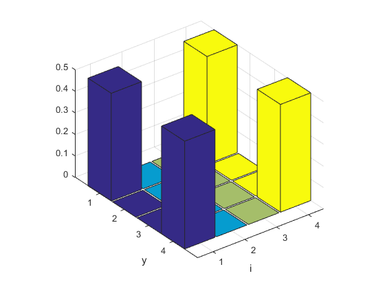
Figure 7: The density matrix $\rho_{1}^{+}=\arrowvert\Phi^{+}\rangle\langle\Phi^{+}\arrowvert$ for the polarized photon entangled states (in the computing basis) obtained from our simulations for advanced model (see details in text).

The considered advanced model has additional important features compared to the simple base models discussed above. One of these features allow us to study a specific quantum entanglement for the mentioned qubits $\arrowvert{p_{i}},n,\lambda_{j}\rangle$ with $i=1,2;j=1,2$ by filtering them from the database $R$ created for the advanced model. It is worth noting that, due to the orthogonality of quantum wavefunctions, only the states with the same spectral numbers $n$ contribute to the entangled qubit states. In follows we will reformat the registered qubits to the Bell’s states BasdevantQM:2005 $(\arrowvert\Phi^{\pm}\rangle,\arrowvert\Psi^{\pm}\rangle)=\arrowvert{p_{i}},n,\lambda_{j}\rangle\pm\arrowvert{p_{i}},n,\lambda_{j}\rangle$ to prepare corresponding density matrices $\rho_{1}^{\pm}$ = ($\arrowvert\Phi^{\pm}\rangle\langle\Phi^{\pm}\arrowvert$, $\rho_{2}^{\pm}$ = ($\arrowvert\Psi^{\pm}\rangle\langle\Psi^{\pm}\arrowvert$. One of such density matrices $\rho_{1}^{+}$ is shown (in the computing basisBasdevantQM:2005 ) in Fig.7. In order to study the entanglement of such states we use a standard technique Wootters:1998 that allow us finding a specific quantity: quantum concurrence $C$. The value $C=1$ indicates the complete two-qubit entanglement in the system. Our calculations (for details see Wootters:1998 ; Burlak:2009 and references therein) show that for considered states the value $C=1$, i.e. corresponding qubits pair are completely entangled.

Conclusion. In our simulations, it is created and used the neural network with following typical parameters: $R_{L}=0.005$, $M_{L}=1$, input numbers $I_{L}=12$, hidden nodes $H_{L}=5$. Our desktop with Core (TM), i3 processor, 8 GB RAM and 3.9 GHz processor, allowed us to achieve the test error $a_{Ts}<2\%$ at the network training by the dataset with $12x2000$ entries for the CPU time less than $1min$. For large databases that were created and analyzed for advanced model (see 3D figures Figs.5, 6) the run-time was about or less $10min$. Considered ML approach may open interesting perspectives at planning of the quantum measurements and the optimal monitoring of complex quantum objects.

Acknowledgment. This work was supported in part by CONACYT (México) under the grants No. A1-S-9201 and No. A1-S-8793.

References

- (1) J. S. Lundeen, B. Sutherland, A. Patel, C. Stewart, C. Bamber, Direct measurement of the quantum wavefunction, Nature, 188, vol. 474 (2011).
- (2) L. Li, Y. Yang, D. Zhang, Zuo-Guang Ye, S. Jesse, S. V. Kalinin, R. K. Vasudevan, Machine learning–enabled identification of material phase transitions based on experimental data, Sci. Adv. 4,( 2018).
- (3) J. Urban, A. Menon, Z. Tian, A. Jain, K. Hippalgaonkar, New horizons in thermoelectric materials: Correlated electrons, organic transport, machine learning, and more, Journal of Applied Physics 125, 180902 (2019).
- (4) D. Vodenicarevic, N. Locatelli, J. Grollier, D. Querlioz, Nano-oscillator-based classification with a machine learning-compatible architecture, Journal of Applied Physics 124, 152117 (2018).
- (5) L. Pilozzi, F. Farrelly, G. Marcucci, C. Conti, Machine learning inverse problem for topological photonics, Comm.phys., 1:57 (2018)
- (6) J. Carrasquilla, R. Melko, Machine learning phases of matter, Nature Physics, 13, 431 (2017).
- (7) J. Salvail, M. Agnew, A. Johnson, E. Bolduc, J. Leach, R. Boyd, Full characterization of polarization states of light via direct measurement, Nature Photonics, 7, 316–321 (2013).
- (8) A. Melnikov, H. Nautrup, M. Krenn, V. Dunjko, M. Tiersch, A. Zeilinger, H. Briegel, Active learning machine learns to create new quantum experiments, PNAS 115 (6) 1221-1226 (2018).
- (9) Vogel, K., Risken, H., Determination of quasiprobability distributions in terms of probability distributions. Phys. Rev. A 40, 2847–2849 (1989).
- (10) Smithey, D. T., Beck, M., Raymer, M. G., Faridani, A. Measurement of the Wigner distribution and the density matrix of a light mode using optical homodyne tomography, Phys. Rev. Lett. 70, 1244–1247 (1993).
- (11) Breitenbach, G., Schiller, S., Mlynek, J. Measurement of the quantum states of squeezed light. Nature 387, 471–475 (1997).
- (12) White, A. G., James, D. F. V., Eberhard, P. H., Kwiat, P. G. Nonmaximally entangled states, Phys. Rev. Lett. 83, 3103–3107 (1999).
- (13) Hofheinz, M. et al. Synthesizing arbitrary quantum states in a superconducting resonator. Nature 459, 546–549 (2009).
- (14) G. Steinbrecher, J. Olson, D. Englund, J.Carolan, Quantum optical neural networks, Npj Quantum Information, 5, 60 (2019).
- (15) J. Schmidhuber, Deep learning in neural networks: An overview, Neural Networks, 61, 85–117 (2015).
- (16) Haykin, S., Neural networks and learning machines, Pearson Education, Inc., Upper Saddle River, New Jersey 07458, 3rd ed. (2009).
- (17) J. Kelleher, B. Mac Namee, A. D’Arcy, Fundamentals of machine learning for predictive data analytics, The MIT Press Cambridge, Massachusetts, London, England, 2015.
- (18) J. McCaffrey, Coding Neural Network Back-Propagation Using C#, https://visualstudiomagazine.com/articles/2015/04/01/back-propagation-using-c.aspx
- (19) L. D. Landau, L. M. Lifshitz, Quantum Mechanics: Non-Relativistic Theory, Butterworth-Heinemann; 3 edition, 1981.
- (20) J. Basdevant, J. Dalibard, Quantum Mechanics, Springer, 2005.
- (21) W. Wootters, Entanglement of Formation of an Arbitrary State of Two Qubits, Phys.Rev.Lett. 80, 10, 2245-2248 (1998).
- (22) G. Burlak, I. Sainz, A. B. Klimov, Entanglement enhancement for two spins assisted by two phase kicks. Phys.Rev. A. 80, 024301 (2009).