Equivalence of wave function matching and Green’s functions methods for quantum transport: generalized Fisher-Lee relation

Abstract

We present a proof of an exact equivalence of the two approaches that are most used in computing conductance in quantum electron and phonon transport: the wave function matching and Green’s functions methods. We can obtain all the quantities defined in one method starting from those obtained in the other. This completes and illuminates the work started Ando[Ando T 1991 Phys. Rev. B 44 8017.] and continued later by Khomyakov et al.[Khomyakov P A , Brocks G, Karpan V, Zwierzycki M and Kelly P J 2005 Phys. Rev. B 72 035450.]. The aim is to allow for solving the transport problem with whichever approach fits most the system at hand. One major corollary of the proven equivalence is our derivation of a generalized Fisher-Lee formula for resolving the transmission function into individual phonon mode contributions. As an illustration, we applied our method to a simple model to highlight its accuracy and simplicity.

Keywords: mesoscopic transport, conductance, wave function matching, Green’s functions

1 Introduction

Electron and phonon transport in mesoscopic systems has gained much interest in the last three decades, due mainly to advances in experimental and computational techniques, as well as the continued improvements in computing resources[3, 4]. Indeed, experimental techniques are nowadays so precise, it has become feasible to wire a nanometric-sized molecule to two metallic leads and measure its transport properties[5]. The technological applications are also varied as a result of the trend to miniaturization, but also the push to exploit the novel effects observed only at the atomic scale. Heat dissipation, Josephson junctions, thermoelectricity, spintronics are among the most prominent applications that rely on such novel phenomena [6, 7, 8, 9]. In general, the setup consists of a central part, the device, considered small, connected to much larger leads. The leads act as heat and particle reservoirs each at a constant temperature an chemical potential. When the leads are kept at slightly different temperatures or chemical potentials, a heat or particle current ensues that passes through the central region. The first attempts at a theoretical understanding of the phenomenon were made in the second half of the last century. We note that when interactions are involved, the heat current in the electronic case is harder to describe. However, in this work we are concerned with the heat transport via harmonic phonons, whose treatment is also similar to the electronic charge transport. Using a phenomenological approach, Landauer[10, 11] expressed the conductance in a two-terminal setup in terms of a transmission probability. There are mainly two methods that are used to compute the latter. The first relies on using wave functions in the electronic case or displacements in the phononic case, and is sometimes known as the wave function matching (WFM) method[1, 12, 13, 14, 15]. The second uses the Green’s function as the main object, and is known as the atomistic Green’s functions method (AGF)[3, 16, 17, 18, 19, 20, 21].

The AGF was first applied to transport by Caroli et al.[22] using a Hamiltonian with a basis of localized wave functions. Their aim was to circumvent the inherently difficult problem of matching correctly the wave functions at the interfaces. Moreover, Green’s functions are the most convenient tool to include correlations in a more realistic treatment of the problem when these are important[9]. The method is also “unique” in that studying systems far from thermal equilibrium relies exclusively on the use of Green’s functions as introduced by the Keldysh formalism [4, 23, 24]. An alternative to the Green’s function method, consists of studying the scattering problem using wave functions. This requires that appropriate boundary conditions be imposed at the interfaces between the scattering central region and the leads. Ando[1] applied the wave function matching method to a tight-binding Hamiltonian, obtaining directly the transmission as well as reflexion probability amplitudes. Ando’s approach was criticized by Krstić et al.[25] for not yielding the correct expression of the conductance, due mainly, as their argument goes, to an inconsistent treatment of the evanescent modes. It is indeed the case that these modes do not participate in the transport, but their inclusion is necessary for a correct matching of the wave functions at the interfaces. Khomyakov et al.[2] later attempted to demonstrate the equivalence between the wave function matching and Green’s functions methods and show that Ando’s approach was correct. Their attempt was successful at deriving the Green’s functions from quantities obtained using the wave functions method. However, finding the complete equivalence remained an open question. Beyond the mere challenge of showing that an equivalence exists, the fallout from such a demonstration is substantial in that one can readily check whether a calculation carried out using either method is corroborated by the other. This is indeed a much needed way to reduce errors, given that the problems tackled are way beyond reach of analytical tools. Moreover, for more realistic calculations one has to appeal to first-principles methods based mostly on the density functional theory(DFT). Most computer codes that implement the DFT make use of the wave function formalism, whereby the appropriate Khon-Sham equations are solved by expanding the electronic wave function on a basis of either localized or extended wave functions[26]. A few other codes rely on the Green’s function formalism[27]. It is, therefore, convenient to implement transport calculations on top of the existing codes using either the WFM or AGF method, depending on the nature of the code, wave-function-based or Green’s-functions-based, and knowing that the results will be identical in either case.

Besides the total transmission function, one major aspect of the whole framework is obtaining mode-resolved transmission probabilities, i.e., individual phonon contributions to the total transmission function [28, 29, 30, 31, 32, 33]. These are important for several reasons. For instance, such detailed information is required as input to other methods used at longer length scales, such as, non-gray Boltzmann equation [28]. One can also consider the interaction between phonons and light, where only the optical branches intervene, hence the need to disentangle their contribution from the rest of the phonon spectrum. The first attempt at deriving these mode-resolved transmissions was contained in the Fisher-Lee relation [34]. Several attempts have been made later on at obtaining such information, but most were misled by the invalid assumption that for a fixed frequency, the eigenvectors are orthogonal [3, 35]. We derive, in the current work, the correct and physically sound generalized Fisher-Lee relation for the mode-resolved transmission probabilities. Aside from the ease of implementation, the final expression which we arrived at has a clear physical interpretation. Previous derivations were obtained through rather involved mathematical machinery[1, 2, 36, 37, 38], and the final expressions, though amenable to our result, still require further manipulations.

In this work we provide a rigorous demonstration of the equivalence of the WFM and the AGF methods by showing that all the quantities calculated within one approach can be readily obtained from the other. These include, for instance, group velocities, transmission probabilities, and the individual phonon contributions to these probabilities. In order to illustrate the concordance, we compare various quantities computed within the two frameworks applied to a simple model. Moreover, we also argue that in order to describe correctly the problem at hand the usual region defined as the central part must include one more atomic plane from each lead.

This paper is organized as follows: In the next section our WFM formalism is introduced and the transmission function is derived within the formalism. In section 3 we provide the equivalence between the WFM and the AGF methods, and derive a generalized Fisher-Lee formula for the mode-resolved transmission amplitudes. In section 4 we apply our method to a simple model and make comparisons with earlier approaches. We finally summarize our main results and discussions in the conclusion.

2 Wave function matching approach

Our main objective is to provide a full correspondence of the two approaches mentioned earlier. We think that the Green’s functions formalism is the more robust, and as such we posit that all the quantities defined in this formalism must be expressible in terms of variables defined in the wave function matching approach. Indeed, the AGF method suffers no ambiguity in defining and computing the various quantities involved in the transport problem. The WFM approach, on the other hand, has been subject to debate as to its correct implementation in the present situation. One chief contention regards the treatment of the decaying modes that result from the presence of the scattering region. In the AGF approach the two main quantities are the retarded and advanced Green’s functions. The first describes outgoing waves from the device, while the second is related to incoming waves. From the mathematical standpoint, an in order to obtain these two quantities from the WFM formalism, we must keep only the evanescent modes that decay away from the device. There is also a compelling physical argument in favor of this choice: the evanescent modes always originate from the device, and can only decay away from it. Besides, if we were to reproduce the asymptotic behavior of the transmission probability, we must not include incoming evanescent modes since they would never reach the device if we inject them far away from it, as is clearly illustrated in Fig. 1.

We begin by reminding the formalism used in studying the scattering problem using matching of the wave functions at the interfaces of a bi-dimensional nano-scale system composed of semi-infinite right and left leads separated with a central device (see Figure 1-a). The leads are considered to be ideal with a periodic potential. The incoming propagating state from the left lead and normal to the interface (say in $x$ direction) is scattered in the device and results in reflected and transmitted propagating as well as evanescent states. In the transverse direction (normal to $x$) the periodicity is assumed to hold. Consequently, the real space components in the transverse direction can be replaced by the normal component of the momentum ($\mathbf{k}_{\perp}$). As is usual we first derive quantities proper to the ideal left and right leads, to be used later to express the transmission probabilities.

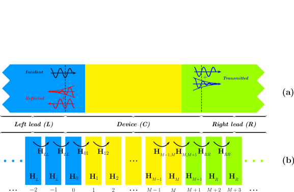
Figure 1: (a) Schematic representation and (b) Hamiltonian matrix divided into slices for the bi-dimensional nano-scale system studied within the WFM approach.

The dynamical matrix of the whole system is given by the following infinite tridiagonal matrix:

$$\mathbf{H}=\left[\begin{array}[]{ccccccc}\ddots&\ddots&0&0&0&0&0\\ \ddots&\mathbf{H}_{L}&\mathbf{H}_{LL}&0&0&0&0\\ 0&\mathbf{H}_{LL}^{\dagger}&\mathbf{H}_{L}&\mathbf{H}_{LL}&0&0&0\\ 0&0&\mathbf{H}_{LL}^{\dagger}&\mathbf{H}_{C}&\mathbf{H}_{RR}&0&0\\ 0&0&0&\mathbf{H}_{RR}^{\dagger}&\mathbf{H}_{R}&\mathbf{H}_{RR}&0\\ 0&0&0&0&\mathbf{H}_{RR}^{\dagger}&\mathbf{H}_{R}&\ddots\\ 0&0&0&0&0&\ddots&\ddots\end{array}\right],$$ (1)

where the indices $L$ and $R$ stand for the left and right leads, respectively, as shown in Fig. 1(b). The part $\mathbf{H}_{C}$ represents the scattering region for which the Hamiltonian matrix is given as

$$\mathbf{H}_{C}=\left[\begin{array}[]{ccccccc}\mathbf{H}_{0}&\mathbf{H}_{01}&0&0&0&0&0\\ \mathbf{H}_{01}^{\dagger}&\mathbf{H}_{1}&\mathbf{H}_{12}&0&0&0&0\\ 0&\mathbf{H}_{12}^{\dagger}&\mathbf{H}_{2}&\ddots&0&0&0\\ 0&0&\ddots&\ddots&\ddots&0&0\\ 0&0&0&\ddots&\mathbf{H}_{M-1}&\mathbf{H}_{M-1,M}&0\\ 0&0&0&0&\mathbf{H}_{M-1,M}^{\dagger}&\mathbf{H}_{M}&\mathbf{H}_{M,M+1}\\ 0&0&0&0&0&\mathbf{H}_{M,M+1}^{\dagger}&\mathbf{H}_{M+1}\end{array}\right].$$ (2)

Here the slides $0$ and $M+1$ are included in the scattering region, although their respective Hamiltonians are seemingly similar to the left and right leads. Indeed, when either the force constants or the masses of the three regions are different, the Hamiltonians $\mathbf{H}_{0}$ and $\mathbf{H}_{M+1}$ are different than $\mathbf{H}_{L}$ and $\mathbf{H}_{R}$, respectively. Because of the assumption that any given slice is connected only to its immediate neighboring slices, the dynamical matrix takes on a tri-diagonal form. As such one atomic slice can be made up of one or more atomic planes, depending on whether interactions are first-neighbor only or are of a longer range (see Fig. 1(b)). The left and right leads are semi-infinite and extend all the way to $-\infty$ and to $+\infty$, respectively.

2.1 Ideal leads

From now on we restrict ourselves to studying the phonon transport, although all the ensuing discussions can be easily carried on to the electronic charge transport. In order to study transport of phonons from one side of the device to the other, we need to first study the motion of phonons in the ideal leads, that is in each lead as if it were infinite in both directions. The eigenmodes of these ideal leads will then be used to study how a phonon sent from the left lead scatters off the central part and results in transmitted and reflected phonons. We begin, therefor, by obtaining the eigenmodes of the ideal leads.

As shown in Figure1-b, the studied system consists of three parts of slices normal to the direction of propagation and indexed from$-\infty$ to $-1$ for the left lead, from $0$ to $M+1$ for the scattering region, and from $M+2$ to $+\infty$ for the right lead. Here we note that one slice from each lead is included as part of the scattering region. The slices are chosen such that only the interactions between neighboring slices are considered.

The equations of motion for the atoms in each ideal lead are given by

$$\omega^{2}\mathbf{u}_{S,i}=\mathbf{H}_{SS}^{\dagger}\,\mathbf{u}_{S,i-1}+\mathbf{H}_{S}\,\mathbf{u}_{S,i}+\mathbf{H}_{SS}\,\mathbf{u}_{S,i+1},$$ (3)

where $\mathbf{H}_{S}$ and $\mathbf{H}_{SS}$ ($S\equiv R$ for the right lead and $S\equiv L$ for the left lead) represent the on-slice and the inter-slice parts of the Hamiltonian, respectively. In this case $i$ runs from $-\infty$ to $+\infty$. It is important to bear in mind that all the Hamiltonian and force constant matrices depend explicitly on $k_{\perp}$, i.e the momentum component which is transverse to the propagation direction $x$. We choose not to show this dependence for the sake of uncluttering the formulae.

They are $N\times N$ matrices, where $N$ is the number of “vibrational degrees of freedom” per slice. In the electronic problem, $N$ is the number of orbitals per slice used as a basis to represent the electronic wave functions. The component of a vibrational mode in slice $i$ is represented by a vector $\mathbf{u}_{S,n}$ of size $N$. The equations of motion can be cast in matrix form as

$$\omega^{2}\left(\begin{array}[]{c}\vdots\\ \mathbf{u}_{S,i-1}\\ \mathbf{u}_{S,i}\\ \mathbf{u}_{S,i+1}\\ \vdots\end{array}\right)=\left[\begin{array}[]{ccccc}\ddots&\ddots&0&0&0\\ \ddots&\mathbf{H}_{S}&\mathbf{H}_{SS}&0&0\\ 0&\mathbf{H}_{SS}^{\dagger}&\mathbf{H}_{S}&\mathbf{H}_{SS}&0\\ 0&0&\mathbf{H}_{SS}^{\dagger}&\mathbf{H}_{S}&\ddots\\ 0&0&0&\ddots&\ddots\end{array}\right]\left(\begin{array}[]{c}\vdots\\ \mathbf{u}_{S,i-1}\\ \mathbf{u}_{S,i}\\ \mathbf{u}_{S,i+1}\\ \vdots\end{array}\right),$$ (4)

For the ideal right lead, where the same unit cell or slice is repeated indefinitely in the $x$ direction of space, we make use of Bloch’s theorem and write ${\displaystyle{\displaystyle\mathbf{u}_{R,i}=e^{iq_{x}\,a_{R}}\,\mathbf{u}_{R,i-1}}}$, where $q_{x}$ and $a_{R}$ are the wave vector and the size of the unit cell in the $x$ direction, respectively. It is important to stress, at this point, that $q_{x}$ can be either a purely real or a complex, having both real and imaginary parts, number. In the latter case the use of the expression “Bloch’s theorem” is a misnomer given that the corresponding modes are not propagating. Defining ${\displaystyle\lambda_{R}=e^{iq_{x}\,a_{R}}}$, we have $\mathbf{u}_{R,i}=\lambda_{R}\,\mathbf{u}_{R,i-1}$. We can now rewrite the equations of motion (3) as

$$\omega^{2}\mathbf{u}_{R,i}=\mathbf{H}_{RR}^{\dagger}\,\lambda_{R}^{-1}\,\mathbf{u}_{R,i}+\mathbf{H}_{R}\,\mathbf{u}_{R,i}+\mathbf{H}_{RR}\,\lambda_{R}\,\mathbf{u}_{R,i}.$$ (5)

That is

$$\left(\omega^{2}-\mathbf{H}_{R}-\lambda_{R}^{-1}\,\mathbf{H}_{RR}^{\dagger}-\lambda_{R}\,\mathbf{H}_{RR}\right)\mathbf{u}_{R,i}=0.$$ (6)

This is a quadratic eigenvalue problem which can be recast as a generalized eigenvalue problem by defining $\lambda_{R}^{-1}\,\mathbf{u}_{R}$ as a new “independent” variable. The new generalized eigenvalue problem then reads

$$\left[\begin{array}[]{cc}\omega^{2}\mathbf{I}-\mathbf{H}_{R}&-\mathbf{H}_{RR}^{\dagger}\\ \mathbf{I}&0\end{array}\right]\left(\begin{array}[]{c}\mathbf{u}_{R}\\ \lambda_{R}^{-1}\,\mathbf{u}_{R}\end{array}\right)=\lambda_{R}\left[\begin{array}[]{cc}\mathbf{H}_{RR}&0\\ 0&\mathbf{I}\end{array}\right]\left(\begin{array}[]{c}\mathbf{u}_{R}\\ \lambda_{R}^{-1}\,\mathbf{u}_{R}\end{array}\right).$$ (7)

Similarly, for the ideal periodic left lead, we have chosen to write, using Bloch’s theorem, $\mathbf{u}_{L,i-1}=\tilde{\lambda}_{L}\,\mathbf{u}_{L,i}$ , where ${\displaystyle\tilde{\lambda}_{L}=e^{-i\,q_{x}\,a_{L}}}$ and $a_{L}$ is the size of the left unit cell. Let us note that the choice of ${\displaystyle\tilde{\lambda}_{L}}$ as the Bloch factor being different from that of the right lead is only motivated by the aim to obtain results that are homogeneous with those obtained through the AGF formalism, as it can be seen later. We can now rewrite Eq. (3) as

$$\omega^{2}\mathbf{u}_{L,n}=\mathbf{H}_{LL}^{\dagger}\,\tilde{\lambda}_{L}\,\mathbf{u}_{L,i}+\mathbf{H}_{L}\,\mathbf{u}_{L,i}+\mathbf{H}_{LL}\,\tilde{\lambda}_{L}^{-1}\,\mathbf{u}_{L,i},$$ (8)

and then

$$\left(\omega^{2}-\mathbf{H}_{L}-\tilde{\lambda}_{L}\,\mathbf{H}_{LL}^{\dagger}-\tilde{\lambda}_{L}^{-1}\,\mathbf{H}_{LL}\right)\mathbf{u}_{L,n}=0.$$ (9)

By defining the new “independent” variable $\tilde{\lambda}_{L}^{-1}\,\mathbf{u}_{L}$, the quadratic eigenvalue problem becomes a generalized eigenvalue problem and reads

$$\left[\begin{array}[]{cc}\omega^{2}\mathbf{I}-\mathbf{H}_{L}&-\mathbf{H}_{LL}\\ \mathbf{I}&0\end{array}\right]\left(\begin{array}[]{c}\mathbf{u}_{L}\\ \tilde{\lambda}_{L}^{-1}\,\mathbf{u}_{L}\end{array}\right)=\tilde{\lambda}_{L}\left[\begin{array}[]{cc}\mathbf{H}_{LL}^{\dagger}&0\\ 0&\mathbf{I}\end{array}\right]\left(\begin{array}[]{c}\mathbf{u}_{L}\\ \tilde{\lambda}_{L}^{-1}\,\mathbf{u}_{L}\end{array}\right).$$ (10)

From (7) and (10), for each value of $\omega$, we obtain $2N$ eigenvalues and eigenvectors for each ideal lead. The eigenmodes are split into two sets of size $N$ each:

1. Right-moving propagating ($\left|\lambda_{R,n}\right|=1\,\mathrm{or}\,\left|\tilde{\lambda}_{L,n}\right|=1\;\textrm{with}\;v_{R/L,n}>0$) and evanescent ($\left|\lambda_{R,n}\right|<1\,\mathrm{or}\,\left|\tilde{\lambda}_{L,n}\right|>1$) modes, where $v_{R/L,n}$ is the group velocity of the $n^{\mathrm{th}}$ mode along the $x$-direction.

2. Left-moving propagating ($\left|\lambda_{R,n}\right|=1\,\mathrm{or}\,\left|\tilde{\lambda}_{L,n}\right|=1\;\textrm{with}\;v_{R/L,n}<0$) and evanescent ($\left|\lambda_{R,n}\right|>1\,\mathrm{or}\,\left|\tilde{\lambda}_{L,n}\right|<1$) modes.

In view of attaching later the leads to the scattering region and having in sight the equivalence with the AGF formalism, we depart from the usual treatments [1, 12, 13, 17] and discard the evanescent modes that decay towards the central region. As mentioned above, the physical justification resides in that evanescent modes are localized around the “defect” and always decay away from it. It does not make sense to include evanescent modes moving towards the “defect”. We also know for a fact that this is indeed the case when using the Green’s functions formalism, and by this clever trick, we will show how to move seamlessly between the two formalisms. And in keeping with the terminology used in the Green’s function formalism, we define quantities built out of these selected evanescent modes and propagating modes moving either towards the defect or away from it. We call the latter “retarded” and the first “advanced”, and in order to differentiate them we append a superscript “a” to the advanced quantities. We note that in what follows the advanced quantities for the right lead are defined only for the sake of completeness. So long as the incoming phonon is injected from the left lead, the boundary conditions are imposed such that there are only transmitted waves in the right lead. These waves are represented by the retarded quantities. As such the advanced quantities are not needed in the right lead. However, if one were to inject phonons from the right lead, then the advanced quantities in the left lead would be the ones to be unused. We begin by reminding the definition of the group velocity:

$$v_{S}=\frac{\partial\omega}{\partial q_{x}}=\frac{1}{2\omega}\frac{\partial\omega^{2}}{\partial q_{x}}.$$ (11)

From the equations of motion in the leads and using the Hellmann-Feynman theorem [39], we obtain the following expressions for the various group velocities defined in the right and left leads:

$$v_{g,R} = \frac{\mathrm{i}\,a_{R}}{2\omega}\left[\mathbf{u}_{R}^{\dagger}\,\mathbf{H}_{RR}\,\mathbf{u}_{R}\,\lambda_{R}-\mathbf{u}_{R}^{\dagger}\,\mathbf{H}_{RR}^{\dagger}\,\mathbf{u}_{R}\,\lambda_{R}^{\dagger}\right],$$ (12)

$$v_{g,R}^{a} = \frac{\mathrm{i}\,a_{L}}{2\omega}\left[\mathbf{u}_{R}^{a\dagger}\,\mathbf{H}_{RR}\,\mathbf{u}_{R}^{a}\,\lambda_{R}^{a}-\mathbf{u}_{R}^{a\dagger}\,\mathbf{H}_{RR}^{\dagger}\,\mathbf{u}_{R}^{a}\,\lambda_{R}^{a\dagger}\right],$$ (13)

$$v_{g,L} = -\frac{\mathrm{i}\,a_{L}}{2\omega}\left[\mathbf{u}_{L}^{\dagger}\,\mathbf{H}_{LL}^{\dagger}\,\mathbf{u}_{L}\,\tilde{\lambda}_{L}-\mathbf{u}_{L}^{\dagger}\,\mathbf{H}_{LL}\,\mathbf{u}_{L}\,\tilde{\lambda}_{L}^{\dagger}\right],$$ (14)

$$v_{g,L}^{a} = -\frac{\mathrm{i}\,a_{L}}{2\omega}\left[\mathbf{u}_{L}^{a\dagger}\,\mathbf{H}_{LL}^{\dagger}\,\mathbf{u}_{L}^{a}\,\tilde{\lambda}_{L}^{a}-\mathbf{u}_{L}^{a\dagger}\,\mathbf{H}_{LL}\,\mathbf{u}_{L}^{a}\,\tilde{\lambda}_{L}^{a\dagger}\right],$$ (15)

where $a_{L}$ and $a_{R}$ are the unit cell size in the left and right leads, respectively. We also define new quantities which are constructed out of the group velocities, with the coefficients ${\displaystyle\frac{a_{L/R}}{2\omega}}$ omitted for convenience when we will be comparing the WFM with the AGF formalisms:

$$\mathbf{V}_{R}=\mathrm{i}\left[\mathbf{C}_{R}^{\dagger}\,\mathbf{H}_{RR}\,\mathbf{C}_{R}\,\mathbf{\boldsymbol{\Lambda}}_{R}-\mathbf{\boldsymbol{\Lambda}}_{R}^{\dagger}\,\mathbf{C}_{R}^{\dagger}\,\mathbf{H}_{RR}^{\dagger}\,\mathbf{C}_{R}\right],$$ (16)

$$\mathbf{V}_{R}^{a}=\mathrm{i}\left[\mathbf{C}_{R}^{a\dagger}\,\mathbf{H}_{RR}\,\mathbf{C}_{R}^{a}\,\mathbf{\boldsymbol{\Lambda}}_{R}^{a}-\mathbf{\boldsymbol{\Lambda}}_{R}^{a\dagger}\,\mathbf{C}_{R}^{a\dagger}\,\mathbf{H}_{RR}^{\dagger}\,\mathbf{C}_{R}^{a}\right],$$ (17)

$$\mathbf{V}_{L}=-\mathrm{i}\left[\mathbf{C}_{L}^{\dagger}\,\mathbf{H}_{LL}^{\dagger}\,\mathbf{C}_{L}\,\mathbf{\boldsymbol{\Lambda}}_{L}-\mathbf{\boldsymbol{\Lambda}}_{L}^{\dagger}\,\mathbf{C}_{L}^{\dagger}\,\mathbf{H}_{LL}\,\mathbf{C}_{L}\right],$$ (18)

$$\mathbf{V}_{L}^{a}=-\mathrm{i}\left[\mathbf{C}_{L}^{a\dagger}\,\mathbf{H}_{LL}^{\dagger}\,\mathbf{C}_{L}^{a}\,\mathbf{\boldsymbol{\Lambda}}_{L}^{a}-\mathbf{\boldsymbol{\Lambda}}_{L}^{a\dagger}\,\mathbf{C}_{L}^{a\dagger}\,\mathbf{H}_{LL}\,\mathbf{C}_{L}^{a}\right].$$ (19)

These matrices are diagonal, with the diagonal elements being the group velocities for the propagating modes, and vanishing for the decaying modes.

We now introduce the matrices built from the eigenvectors and eigenmodes of the ideal leads that will be used in the WFM formalism to obtain the vibration modes in the central region. For the right lead, we define

$$\mathbf{C}_{R}=\left(\mathbf{u}_{R,1},\mathbf{u}_{R,2},\cdots,\mathbf{u}_{R,n}\right),$$ (20)

$$\mathbf{C^{\mathrm{\mathit{a}}}}_{R}=\left(\mathbf{u}_{R,1}^{a},\mathbf{u}_{R,2}^{a},\cdots,\mathbf{u}_{R,n}^{a}\right),$$ (21)

$$\boldsymbol{\Lambda}_{R}=\mathrm{diag}\left(\lambda_{R,1},\lambda_{R,2},\cdots,\lambda_{R,n}\right),$$ (22)

and

$$\boldsymbol{\Lambda}_{R}^{a}=\mathrm{diag}\left(\lambda_{R,1}^{a},\lambda_{R,2}^{a},\cdots,\lambda_{R,n}^{a}\right),$$ (23)

and we define similar quantities for the left lead with $\lambda_{R}$ replaced by $\tilde{\lambda}_{L}$, and $\mathbf{u}_{R}$ by $\mathbf{u}_{L}$.

2.2 The scattering region

We now proceed to writing the effective Hamiltonian of the scattering region, replacing the effects of the ideal leads by “self-energy” terms to be added to the original Hamiltonian. Writing the equation of motion for slice $0$,

$$\mathbf{-H}_{LL}^{\dagger}\mathbf{\mathbf{u}_{\mathrm{-1}}\mathbf{+}\mathrm{(}\omega^{2}\mathbf{I}-H}_{0})\mathbf{\mathbf{u}_{\mathrm{0}}-H}_{01}\mathbf{u}_{1}=0,$$

and moving the first term to the right-hand side, we have

$$\mathbf{\mathrm{(}\omega^{2}\mathbf{I}-H}_{0})\mathbf{\mathbf{u}_{\mathrm{0}}-H}_{01}\mathbf{u}_{1}=\mathbf{H}_{LL}^{\dagger}\mathbf{u}_{-1}.$$

In a similar fashion, we find for slice $M+1$,

$$\mathbf{\mathrm{(}\omega^{2}\mathbf{I}-H}_{M+1})\mathbf{\mathbf{u}_{\mathrm{M+1}}-H}_{M,M+1}\mathbf{u}_{M}=\mathbf{H}_{RR}\mathbf{u}_{M+2}.$$

The equations of motion for the central part are then given in matrix form as

$$\left[\omega^{2}\mathbf{I}-\mathbf{H}_{C}\right]\left[\begin{array}[]{c}\mathbf{u}_{0}\\ \mathbf{u}_{1}\\ \\ \vdots\\ \\ \mathbf{u}_{M}\\ \mathbf{u}_{M+1}\end{array}\right]=\left[\begin{array}[]{c}\mathbf{\mathbf{H}_{LL}^{\dagger}u}_{-1}\\ 0\\ 0\\ \vdots\\ 0\\ 0\\ \mathbf{\mathbf{H}_{RR}u}_{M+2}\end{array}\right],$$ (24)

with the full matrix form of $\mathbf{H}_{C}$ given in Eq. 2.

This means that if we know or impose the values of $\mathbf{u}_{-1}$ and $\mathbf{u}_{M+2},$ we can invert this matrix equation to obtain all the displacement $\mathbf{u}_{i},$ with $i=0,1,...,M+1$.

To accomplish this, we make use of Bloch’s theorem which holds in the leads. We write

$$\left\{\begin{array}[]{lr}\mathbf{u}_{-1}=&{\displaystyle\tilde{\lambda}_{L}\mathbf{u}_{0}}\quad\textrm{with}\quad\tilde{\lambda}=e^{-i\,q_{x}a_{L}},\\ \mathbf{u}_{M+2}=&{\displaystyle\lambda_{R}\,\mathbf{u}_{M+1}}\quad\textrm{with}\quad\lambda_{R}=e^{i\,q_{x}a_{R}}\end{array}\right.,$$ (25)

Imposing an incoming mode from the left lead, with an amplitude $\mathbf{a}_{in}$ , the displacement $\mathbf{u}_{0}$ will be a linear combination of the incoming and reflected waves. In the right lead we impose that only the transmitted wave exist. We have then

$$\left\{\begin{array}[]{lr}\mathbf{u}_{0}=&\mathbf{C}_{L}^{a}\,\mathbf{a}_{in}+\mathbf{C}_{L}\,\mathbf{a}_{ref},\\ \mathbf{u}_{M+1}=&\mathbf{C}_{R}\,\mathbf{a}_{tr}\end{array}\right.,$$ (26)

where the vector $\mathbf{a}_{in}$ is the amplitude of the right-going incoming wave, $\mathbf{a}_{ref}$ is the amplitude of the reflected wave, and $\mathbf{a}_{tr}$ is the amplitude of the transmitted wave. The latter two vectors are to be calculated given the boundary conditions. The first boundary condition is given by setting the vector $\mathbf{a}_{in}$. This is usually taken as a unit vector, whose components are all zero, except for the component, corresponding to one mode, which is set to unity. The second “boundary condition” imposed on the wave function is that the left-going part in the right lead vanishes.

Making use of Bloch’s theorem, we have

$$\left\{\begin{array}[]{lr}\mathbf{u}_{-1}=&\mathbf{C}_{L}^{a}\,\boldsymbol{\Lambda}_{L}^{a}\mathbf{a}_{in}+\mathbf{C}_{L}\,\boldsymbol{\Lambda}_{L}\mathbf{a}_{ref},\\ \mathbf{u}_{M+2}=&\mathbf{C}_{R}\,\boldsymbol{\Lambda_{R}}\mathbf{a}_{tr}\end{array}\right..$$ (27)

We introduce the pseudo-inverse matrices $\tilde{\mathbf{C}_{L}}$, $\tilde{\mathbf{C}_{L}^{a}}$, and $\tilde{\mathbf{C}_{R}}$ such that $\tilde{\mathbf{C}_{L}}\mathbf{C}_{L}=\mathbf{I}$, $\tilde{\mathbf{C}_{L}^{a}}\mathbf{C}_{L}^{a}=\mathbf{I}$, and $\tilde{\mathbf{C}_{R}}\mathbf{C}_{R}=\mathbf{I}$, where $\mathbf{I}$ is the $n\times n$ identity matrix. Using these matrices, the wave function component $\mathbf{u}_{-1}$ is expressed as

$$\mathbf{u}_{-1}=\mathbf{\mathbf{C}}_{L}^{a}\,\mathbf{\boldsymbol{\Lambda}}_{L}^{a}\,\tilde{\mathbf{C}}_{L}^{a}\,\mathbf{C}_{L}^{a}\,\mathbf{a}_{in}+\mathbf{C}_{L}\,\boldsymbol{\Lambda}_{L}\,\tilde{\mathbf{C}}_{L}\,\mathbf{C}_{L}\mathbf{a}_{ref},$$

and given that $\mathbf{C}_{L}\mathbf{a}_{ref}=\mathbf{u}_{0}-\mathbf{C}_{L}^{a}\,\mathbf{a}_{in}$, we have

$$\mathbf{u}_{-1}=\mathbf{\mathbf{C}}_{L}^{a}\,\boldsymbol{\Lambda}_{L}^{a}\,\tilde{\mathbf{C}}_{L}^{a}\,\mathbf{C}_{L}^{a}\,\mathbf{a}_{\mathrm{in}}+\mathbf{C}_{L}\,\mathbf{\mathbf{\boldsymbol{\Lambda}}}_{L}\,\tilde{\mathbf{C}}_{L}\left(\mathbf{u}_{0}-\mathbf{C}_{L}^{a}\,\mathbf{a}_{\mathrm{in}}\right).$$

Introducing the Bloch matrices

$$\mathbf{B}_{L}=\mathbf{C}_{L}\,\mathbf{\boldsymbol{\Lambda}}_{L}\,\tilde{\mathbf{C}}_{L}$$ (28)

and

$$\mathbf{B}_{L}^{a}=\mathbf{\mathbf{C}}_{L}^{a}\,\boldsymbol{\Lambda}_{L}^{a}\,\tilde{\mathbf{C}}_{L}^{a},$$ (29)

we obtain

$$\mathbf{u}_{-1}=\mathbf{B}_{L}^{a}\,\mathbf{C}_{L}^{a}\,\mathbf{a}_{in}+\mathbf{B}_{L}\,\mathbf{u}_{0}-\mathbf{B}_{L}\,\mathbf{C}_{L}^{a}\,\mathbf{a}_{\mathrm{in}},$$ (30)

and finally

$$\mathbf{u}_{-1}=\left(\mathbf{B}_{L}^{a}-\mathbf{B}_{L}\right)\mathbf{C}_{L}^{a}\,\mathbf{a}_{\mathrm{in}}+\mathbf{B}_{L}\,\mathbf{u}_{0}.$$ (31)

Similarly for the right lead, we introduce the Bloch matrix

$$\mathbf{B}_{R}=\mathbf{C}_{R}\,\boldsymbol{\Lambda}_{R}\,\tilde{\mathbf{C}}_{R},$$ (32)

and write

$$\mathbf{u}_{M+2}=\mathbf{C}_{R}\,\boldsymbol{\Lambda}_{R}\,\tilde{\mathbf{C}}_{R}\,\mathbf{C}_{R}\,\mathbf{a}_{tr}=\mathbf{B}_{R}\,\mathbf{C}_{R}\,\mathbf{a}_{tr}=\mathbf{B}_{R}\,\mathbf{u}_{M+1}.$$ (33)

Using the above, we finally obtain the following system of equations for the central part

$$(\omega^{2}\mathbf{I}-\boldsymbol{\mathbf{H}}_{eff}^{W})\left[\begin{array}[]{c}\mathbf{u}_{0}\\ \vdots\\ \vdots\\ \mathbf{u}_{M+1}\end{array}\right]=\left[\begin{array}[]{c}\mathbf{q}_{\mathrm{inj}}\\ 0\\ \vdots\\ 0\end{array}\right],$$

with

$$\mathbf{H}_{eff}^{W}=\left[\begin{array}[]{ccccccc}\mathbf{H}_{LS}&\mathbf{H}_{01}&0&0&0&0&0\\ \mathbf{H}_{01}^{\dagger}&\mathbf{H}_{1}&\mathbf{H}_{12}&0&0&0&0\\ 0&\mathbf{H}_{12}^{\dagger}&\mathbf{H}_{2}&\ddots&0&0&0\\ 0&0&\ddots&\ddots&\ddots&0&0\\ 0&0&0&\ddots&\mathbf{H}_{M-1}&\mathbf{H}_{M-1,M}&0\\ 0&0&0&0&\mathbf{H}_{M-1,M}^{\dagger}&\mathbf{H}_{M}&\mathbf{H}_{M,M+1}\\ 0&0&0&0&0&\mathbf{H}_{M,M+1}^{\dagger}&\mathbf{H}_{RS}\end{array}\right],$$ (34)

$$\mathbf{H}_{LS}=\mathbf{H}_{0}+\mathbf{H}_{LL}^{\dagger}\mathbf{B}_{L},$$

$$\mathbf{H}_{RS}=\mathbf{H}_{M+1}+\mathbf{H}_{RR}\mathbf{B}_{R},$$

and

$$\mathbf{q}_{\mathrm{inj}}=\mathbf{H}_{LL}^{\dagger}\left(\mathbf{B}_{L}^{a}-\mathbf{B}_{L}\right)\mathbf{C}_{L}^{a}\mathbf{a}_{in}.$$

The quantities

$$\Sigma_{R}^{W}=\mathbf{H}_{RR}\mathbf{B}_{R}$$ (35)

and

$$\Sigma_{L}^{W}=\mathbf{H^{\dagger}}_{LL}\mathbf{B}_{L}$$ (36)

are known, respectively, as the self-energies for the right and left leads, and are formally introduced later in the AGF formalism. These are the defining quantities that will allow us to establish a connection with the AGF method and, consequently, the sought after equivalence. Defining $\mathbf{G}_{C}^{W}=\left[\omega^{2}\mathbf{I}-\boldsymbol{\mathbf{H}}_{eff}^{W}\right]^{-1}$, the above system can inverted as

$$\left[\begin{array}[]{c}\mathbf{u}_{0}\\ \vdots\\ \vdots\\ \mathbf{u}_{M+1}\end{array}\right]=\boldsymbol{\mathbf{G}}_{C}^{W}\left[\begin{array}[]{c}\mathbf{q}_{\mathrm{inj}}\\ 0\\ \vdots\\ 0\end{array}\right].$$ (37)

We remark at this point that only the three Bloch matrices ($\mathbf{B}_{L}$, $\mathbf{B}_{L}^{a}$, and $\mathbf{B}_{R}$) we defined above are needed to carry out all the subsequent analyses and computations. As we will see below, these matrices can all be obtained from the AGF approach. However, it is customary in prior literature[2, 30] to define eight such matrices, with four of them having no connection at all to the AGF formalism.

2.3 Transmission

For a particular incoming mode $m$ given by the $m^{\mathrm{th}}$ column of the matrix $\mathbf{C}_{L}^{a}$, the expression $\mathbf{u}_{M+1}=\mathbf{C}_{R}\,\mathbf{a}_{tr}$ reads:

$$\mathbf{C}_{R}\,\boldsymbol{\tau}_{m}=\mathbf{u}_{M+1,m}.$$ (38)

We define the matrix $\boldsymbol{\tau}$ as composed of the columns $\tau_{m}$($m=1,2,...,N$), where $N$ is the number of modes:

$$\boldsymbol{\boldsymbol{\tau}}=(\boldsymbol{\tau}_{1}\,\boldsymbol{\tau}_{2}\,...\,\boldsymbol{\tau}_{N}).$$

We generalize the earlier relation and obtain

$$\mathbf{C}_{R}\,\boldsymbol{\tau}=(\mathbf{u}_{M+1,1}\,\mathbf{u}_{M+1,2}\,....\,\mathbf{u}_{M+1,N}).$$

From Eq. 37, we have

$$\mathbf{u}_{M+1,m}=\mathbf{G}_{C}^{W}(M+1,0)\mathbf{q}_{\mathrm{inj}}.$$ (39)

It is a common practice to fix $\mathbf{a}_{in}$ as having a unit component only along the $m^{\mathrm{{th}}}$mode, with all the other components vanishing. Instead of working with the vectors $\mathbf{a}_{in}$ and $\mathbf{q}_{inj}$, we define the respective matrices $\mathbf{A}_{in}$ and $\mathbf{Q}_{inj}$. Here $\mathbf{A}_{in}$ is just the $n\times n$ identity matrix, and as a consequence, $\mathbf{Q}_{inj}$ is given as

$$\mathbf{Q}_{\mathrm{inj}}=\mathbf{H}_{LL}^{\dagger}(\mathbf{B}_{L}^{a}-\mathbf{B}_{L})\mathbf{C}_{L}^{a}\mathbf{A}_{in}=\mathbf{H}_{LL}^{\dagger}(\mathbf{B}_{L}^{a}-\mathbf{B}_{L})\mathbf{C}_{L}^{a},$$ (40)

which follows from $\mathbf{A}_{in}$ being the identity matrix. We then obtain

$$\tau=\mathbf{C}_{R}^{-1}\mathbf{G}_{C}^{W}(M+1,0)\mathbf{Q}_{\mathrm{inj}}.$$

The transmission amplitude is therefore found by normalizing with respect to the current and reads

$$\mathbf{t}= \mathbf{V}_{R}^{\nicefrac{{1}}{{2}}}\,\mathbf{C}_{R}^{-1}\,\mathbf{G}_{C\left(M+1,0\right)}^{W}\,\mathbf{Q}_{\mathrm{inj}}\,\left(\mathbf{V}_{L}^{a}\right)^{\nicefrac{{-1}}{{2}}}.$$

Replacing $\mathbf{Q}_{\mathrm{inj}}$ , defined in Eq. (eq. 40), with its alternative expression, $\mathbf{Q}_{\mathrm{inj}}=i\left(\mathbf{C}_{L}^{a\dagger}\right)^{-1}\mathbf{V}_{L}^{a}$(cf. B), we arrive at the final expression for the transmission amplitude:

$$\mathbf{t}=i\,\mathbf{V}_{R}^{\nicefrac{{1}}{{2}}}\,\mathbf{C}_{R}^{-1}\,\mathbf{G}_{C\left(M+1,0\right)}^{W}\left(\mathbf{C}_{L}^{a\dagger}\right)^{-1}\left(\mathbf{V}_{L}^{a}\right)^{\nicefrac{{1}}{{2}}}.$$ (41)

This is similar to the expression arrived at by Komyakov et al.[2], starting from the AGF formalism. The difference lies in the way they define the Bloch matrix describing the incoming wave. As a result, in their case, even the evanescent modes yield non-vanishing elements in $\mathbf{Q}_{\mathrm{inj}}$, which they then proceed to eliminate “by hand”, by considering the group velocities. The evanescent modes, having a vanishing group velocity, the corresponding entries in $\mathbf{Q}_{\mathrm{inj}}$ are set to zero. However, in our case the evanescent modes are eliminated “naturally” thanks to the clever choice of the modes entering our definition of the Bloch matrix $\mathbf{B}_{L}^{a}$. By naturally we mean that there is no need to scan over the modes is search of the decaying ones and then zero out the corresponding entries in $\mathbf{Q}_{inj}$.We must indicate that Komyakov et al.[2] define a matrix $\mathbf{Q}_{0}$ (their eq. 14), which when multiplied by their $\mathbf{U}_{L}(+)$ (their eq. 55) on the right, yields a matrix $\mathbf{Q}_{\mathrm{inj}}^{\mathrm{K}}$, to which we compare our $\mathbf{Q}_{\mathrm{inj}}$.

3 AGF formalism

3.1 A brief review of the conventional AGF formalism

We now provide a brief overview of the well-known AGF method with the aim to demonstrate its equivalence the WFM formalism described earlier. And more importantly, once the complete equivalence is shown, we will exploit it to extract the individual, i.e. mode-resolved transmission amplitudes. For a more detailed treatment of the AGF method, we refer the reader to prior literature [40, 41].

In the single particle formalism the retarded Green’s function $\mathbf{G}$ , also known as the resolvent, is defined as the operator inverse of the Hamiltonian $\mathbf{H}$ (given in Eq. 1):

$$(\omega^{2}\mathbf{I}+i\eta-\mathbf{H})\mathbf{G}(\omega,\mathbf{k}_{\perp})=\mathbf{I},$$

where $\eta$ is a positive infinitesimal. A similar equation with $-i\eta$ (instead of $+i\eta$) defines the advanced Green’s function $\mathbf{G}^{a}$, which can also be viewed as the conjugate of the retarded function $\mathbf{G}$. The element $\mathbf{G}_{ij}$ represents the response of slice $j$ to a small vibration of slice $i$. It is therefore related to the transmission probability between slices $i$ and $j$. In matrix form, the above equation reads

$$\left[\begin{array}[]{ccc}\omega^{2}\mathbf{I}-\mathbf{H}_{L}&-\mathbf{H}_{LL}&0\\ -\mathbf{H}_{LL}^{\dagger}&\omega^{2}\mathbf{I}-\mathbf{H}_{C}&-\mathbf{H}_{RR}\\ 0&-\mathbf{H}_{RR}^{\dagger}&\omega^{2}\mathbf{I}-\mathbf{H}_{R}\end{array}\right]\left[\begin{array}[]{ccc}\mathbf{G}_{L}&\mathbf{G}_{LC}&\mathbf{G}_{LR}\\ \mathbf{G}_{CL}&\mathbf{G}_{C}&\mathbf{G}_{CR}\\ \mathbf{G}_{RL}&\mathbf{G}_{RC}&\mathbf{G}_{R}\end{array}\right]=\left[\begin{array}[]{ccc}\mathbf{I}&0&0\\ 0&\mathbf{I}&0\\ 0&0&\mathbf{I}\end{array}\right].$$

We can then solve for the central part alone and obtain

$$\mathbf{G}_{C}=\left[\omega^{2}\mathbf{I}-\mathbf{H}_{C}-\mathbf{\boldsymbol{\Sigma}}_{L}-\boldsymbol{\Sigma}_{R}\right]^{-1},$$

where $\boldsymbol{\Sigma}_{L}$ and $\boldsymbol{\Sigma}_{R}$ are the self-energies containing the effects due to connecting the central region to the left and right leads, respectively. They are given by

$$\boldsymbol{\Sigma}_{L}=\mathbf{H}_{LL}^{\dagger}\,\mathbf{g}_{L}\,\mathbf{H}_{LL},$$ (42)

and

$$\mathbf{\boldsymbol{\Sigma}}_{R}=\mathbf{H}_{RR}\,\mathbf{g}_{R}\,\mathbf{H}_{RR}^{\dagger},$$ (43)

where $\mathbf{g}_{L}$ and $\mathbf{g}_{R}$ are the surface Green’s functions of the left and right leads, respectively[40, 41]. In this work they are computed using a numerically efficient algorithm devised by Lopez-Sancho[42, 43, 24]. The central part is as such represented by an effective Hamiltonian

$$\mathbf{H}_{eff}^{G}=\left[\begin{array}[]{ccccccc}\mathbf{H}_{0}+\boldsymbol{\Sigma}_{L}&\mathbf{H}_{01}&0&0&0&0&0\\ \mathbf{H}_{01}^{\dagger}&\mathbf{H}_{1}&\mathbf{H}_{12}&0&0&0&0\\ 0&\mathbf{H}_{12}^{\dagger}&\mathbf{H}_{2}&\ddots&0&0&0\\ 0&0&\ddots&\ddots&\ddots&0&0\\ 0&0&0&\ddots&\mathbf{H}_{M-1}&\mathbf{H}_{M-1,M}&0\\ 0&0&0&0&\mathbf{H}_{M-1,M}^{\dagger}&\mathbf{H}_{M}&\mathbf{H}_{M,M+1}\\ 0&0&0&0&0&\mathbf{H}_{M,M+1}^{\dagger}&\mathbf{H}_{M+1}+\boldsymbol{\Sigma}_{R}\end{array}\right],$$ (44)

such that

$$(\omega^{2}\mathbf{I}-\mathbf{H}_{eff}^{G})\mathbf{G}_{C}=\mathbf{I}.$$

The device Green’s functions $\mathbf{G}_{C}$ and $\mathbf{G}_{C}^{a}$ are then used to compute the total transmission via the Caroli formula [22]:

$$T=\mathrm{trace}\left(\mathbf{G_{\mathrm{C}}}\,\mathbf{\boldsymbol{\Gamma}}_{L}\,\mathbf{G_{\mathrm{C}}^{\mathit{a}}}\,\mathbf{\boldsymbol{\Gamma}}_{R}\right),$$ (45)

where

$$\mathbf{\boldsymbol{\Gamma}}_{R(L)}=i\left(\mathbf{\boldsymbol{\Sigma}}_{R(L)}-\mathbf{\boldsymbol{\Sigma}}_{R(L)}^{\dagger}\right).$$

3.2 Equivalence of WFM and AGF

The effective Hamiltonian $\mathbf{H}_{eff}^{G}$ defined in Eq. 44 is to be compared to the effective Hamiltonian $\mathbf{H}_{eff}^{W}$ obtained in the WFM formalism (Eq. 34). The two must indeed be identical. As a result, we can now proceed to identifying the elements appearing in the two expressions of the effective Hamiltonian. The right and left self-energies pertaining to the effects of the right and left leads, respectively, in the WFM formalism are given in Eqs. 35 and 36. The equivalent quantities given in the AGF formalism are written in Eqs. 42 and 43. Equating these quantities term by term leads to the following equivalences

$$\mathbf{B}_{R} = \mathbf{g}_{R}\,\mathbf{H}_{RR}^{\dagger},$$ (46)

$$\mathbf{B}_{L} = \mathbf{g}_{L}\,\mathbf{H}_{LL}.$$ (47)

The surface Green’s functions are then related to the Bloch matrices as

$$\mathbf{g}_{R} = \mathbf{B}_{R}\,\left(\mathbf{H}_{RR}^{\dagger}\right)^{-1},$$ (48)

$$\mathbf{g}_{L} = \mathbf{B}_{L}\,\left(\mathbf{H}_{LL}\right)^{-1},$$ (49)

for the right and left leads, respectively. Similarly, for the advanced quantities, the self-energies are given in the WFM formalism as

$$\mathbf{\boldsymbol{\Sigma}}_{R}^{a(W)} = \mathbf{H}_{RR}\,\mathbf{B}_{R}^{a},$$ (50)

$$\mathbf{\boldsymbol{\Sigma}}_{L}^{a(W)} = \mathbf{H}_{LL}^{\dagger}\,\mathbf{B}_{L}^{a},$$ (51)

and in the AGF formalism as

$$\mathbf{\boldsymbol{\Sigma}}_{R}^{a} = \mathbf{H}_{RR}\,\mathbf{g}_{R}^{a}\,\mathbf{H}_{RR}^{\dagger},$$ (52)

$$\mathbf{\boldsymbol{\Sigma}}_{L}^{a} = \mathbf{H}_{LL}^{\dagger}\,\mathbf{g}_{L}^{a}\,\mathbf{H}_{LL}.$$ (53)

Equating these quantities leads to the following equivalences

$$\mathbf{B}_{R}^{a} = \mathbf{g}_{R}^{a}\,\mathbf{H}_{RR}^{\dagger},$$ (54)

$$\mathbf{B}_{L}^{a} = \mathbf{g}_{L}^{a}\,\mathbf{H}_{LL}.$$ (55)

The advanced surface GFs are then related to the advanced Bloch matrices as

$$\mathbf{g}_{R}^{a} = \mathbf{B}_{R}^{a}\left(\mathbf{H}_{RR}^{\dagger}\right)^{-1},$$ (56)

$$\mathbf{g}_{L}^{a} = \mathbf{B}_{L}^{a}\left(\mathbf{H}_{LL}\right)^{-1}.$$ (57)

Finally, we arrive at the following expressions for the normalized group velocity matrices needed in the expression of the transmission amplitudes:

$$\begin{array}[]{ccc}\mathbf{V}_{R}&=&\mathbf{C}_{R}^{\dagger}\,\Gamma_{R}\,\mathbf{C}_{R,}\\ \mathbf{V}_{L}^{a}&=&\mathbf{C}_{L}^{a\dagger}\,\Gamma_{L}\,\mathbf{C}_{L}^{a}.\end{array}$$ (58)

with the details given in A. These are identical to the expressions found by Komyakov et al.[12] who used a rather complicated route. We note that these are the key ingredients to resolving, in the next sub-section, the total transmission function in terms of individual phonon contributions. But, before moving on, we think it is important to keep track of the most important quantities introduced so far within the two approaches. These are shown in Table 1 and in the order that they are computed in each method.

WFM	AGF
$H_{L}$, $H_{R}$	$H_{L}$, $H_{R}$
$B_{L}$, $B_{L}^{a}$, $B_{R}$	$g_{L}$, $g_{R}$
$\Sigma_{L}^{W}$,$\Sigma_{R}^{W}$	$\Sigma_{L}$,$\Sigma_{R}$
$H_{C}^{W}$	$H_{C}$
$\left(H_{C}^{W}\right)^{-1}\equiv G_{C}^{W}$	$H_{C}^{-1}\equiv G_{C}$
$T$	$T$

Table 1: A comparative list of the quantities defined in the two formalisms, WFM and AGF, and in the same order of their calculations.

3.3 Mode-resolved transmissions

As mentioned earlier, a number of attempts were made aiming at deriving expressions[2, 28, 29, 30, 32, 37] for the mode-resolved transmission probabilities. However, these reports were based on involved mathematical derivations and it is not yet obvious whether all agree in the end. In our case, we will exploit the identities in Eq. 58 for a straightforward derivation of the desired relation.One advantage of our derivation is that it yields to a straightforward physical interpretation.

Indeed, we can obtain $\Gamma_{R}$ and $\Gamma_{L}$ in terms of the normalized group velocity matrices form Eq. 58 as:

$$\mathbf{\boldsymbol{\Gamma}}_{R}=\left(\mathbf{C}_{R}^{\dagger}\right)^{-1}\,\mathbf{V}_{R}\,\left(\mathbf{C}_{R}\right)^{-1}$$ (59)

and

$$\mathbf{\boldsymbol{\Gamma}}_{L}=\left(\mathbf{C}_{L}^{a\dagger}\right)^{-1}\,\mathbf{V}_{L}^{a}\,\left(\mathbf{C}_{L}^{a}\right)^{-1}.$$ (60)

Next, we define the following operators:

$$\boldsymbol{\Pi}_{R}=\left(\mathbf{C}_{R}^{\dagger}\right)^{-1}\,\left(\mathbf{V}_{R}\right)^{\nicefrac{{1}}{{2}}}$$ (61)

and

$$\boldsymbol{\Pi}_{L}=\left(\mathbf{C}_{L}^{a\dagger}\right)^{-1}\,\left(\mathbf{V}_{L}^{a}\right)^{\nicefrac{{1}}{{2}}},$$ (62)

such that

$$\boldsymbol{\Pi}_{R}\,\boldsymbol{\Pi}_{R}^{\dagger}=\left(\mathbf{C}_{R}^{\dagger}\right)^{-1}\,\mathbf{V}_{R}\,\left(\mathbf{C}_{R}\right)^{-1}=\mathbf{\boldsymbol{\Gamma}}_{R},$$

and

$$\boldsymbol{\Pi}_{L}\,\boldsymbol{\Pi}_{L}^{\dagger}=\left(\mathbf{C}_{L}^{a\dagger}\right)^{-1}\,\mathbf{V}_{L}^{a}\,\left(\mathbf{C}_{L}^{a}\right)^{-1}=\mathbf{\boldsymbol{\Gamma}}_{L}.$$

The Caroli formula (Eq. 45) can now be recast as

$$T= \mathrm{trace}\left(\mathbf{G}^{r}\,\mathbf{\boldsymbol{\Gamma}}_{L}\,\mathbf{G}^{a}\,\mathbf{\boldsymbol{\Gamma}}_{R}\right)$$

$$= \mathrm{trace}\left(\mathbf{G}^{r}\,\boldsymbol{\Pi}_{L}\,\boldsymbol{\Pi}_{L}^{\dagger}\,\mathbf{G}^{a}\,\boldsymbol{\Pi}_{R}\,\boldsymbol{\Pi}_{R}^{\dagger}\right)$$

$$= \mathrm{trace}\left(\boldsymbol{\Pi}_{R}^{\dagger}\,\mathbf{G}^{r}\,\boldsymbol{\Pi}_{L}\,\boldsymbol{\Pi}_{L}^{\dagger}\,\mathbf{G}^{a}\,\boldsymbol{\Pi}_{R}\right)$$

$$= \mathrm{trace}\left(\mathbf{t}\,\mathbf{t}^{\dagger}\right),$$ (63)

where we made use of the cyclic property of the trace. We can identify the matrices appearing in the last line of the equality as

$$\mathbf{t}=i\boldsymbol{\,\Pi}_{R}^{\dagger}\,\mathbf{G}_{C}\,\boldsymbol{\Pi}_{L}=i\;\left(\mathbf{V}_{R}\right)^{\nicefrac{{1}}{{2}}}\,\left(\mathbf{C}_{R}\right)^{-1}\mathbf{G}_{C}\,\left(\mathbf{C}_{L}^{a\dagger}\right)^{-1}\,\left(\mathbf{V}_{L}^{a}\right)^{\nicefrac{{1}}{{2}}},$$ (64)

and

$$\mathbf{t}^{\dagger}=-i\boldsymbol{\,\Pi}_{L}^{\dagger}\,\mathbf{G}_{C}^{a}\,\boldsymbol{\Pi}_{R}=-i\;\left(\mathbf{V}_{L}^{a}\right)^{\nicefrac{{1}}{{2}}}\,\left(\mathbf{C}_{L}^{a}\right)^{-1}\mathbf{G}_{C}^{a}\,\left(\mathbf{C}_{R}^{\dagger}\right)^{-1}\,\left(\mathbf{V}_{R}\right)^{\nicefrac{{1}}{{2}}}.$$

We note that the matrices $\mathbf{C}_{R}$ and $\mathbf{C}_{L}^{a}$ can be readily obtained from the Green’s functions as shown in C. We can clearly see that the transmission matrix given by Eq. 64 is identical to its definition in the WFM formalism (Eq. 41), with the identity $\boldsymbol{\mathbf{G}}_{C}^{W}\equiv\boldsymbol{\mathbf{G}}_{C}$. The mode-resolved transmissions, say from mode $m$ in the left lead to mode $k$ in the right lead, are given as the matrix elements

$$t_{k,m}=\left\{i\,\mathbf{V}_{R}^{\nicefrac{{1}}{{2}}}\,\mathbf{C}_{R}^{-1}\,\mathbf{G}_{C}\left(\mathbf{C}_{L}^{a\dagger}\right)^{-1}\,\left(\mathbf{V}_{L}^{a}\right)^{\nicefrac{{1}}{{2}}}\right\}_{k,m}.$$ (65)

This expression gives the correct mode-resolved transmission functions, but one has to perform all the matrix operations involved in obtaining $t$. It would be convenient to derive a simpler expression where matrix elements could be computed without the unnecessary computational overhead of these matrix operations. In order to derive the desired expression, we multiply both sides of the identities given in Eqs. 59 and 60, by $\mathbf{V_{\mathit{R}}^{\mathrm{\mathit{\mathrm{-1/2}}}}C}_{R}^{\dagger}$ on the right and by $\boldsymbol{C}_{L}^{a}\left(\mathbf{V}_{L}^{a}\right)^{\mathrm{-1/2}}$ on the left, respectively, and obtain

$$\begin{array}[]{ccc}\mathbf{V_{\mathit{R}}^{\mathrm{\mathit{\mathbf{\mathrm{-1/2}}}}}C}_{R}^{\dagger}\,\boldsymbol{\Gamma}_{R}&=&\mathbf{V^{\mathit{1/2}}}_{R}\,\mathbf{C}_{R}^{-1},\\ \boldsymbol{\Gamma}_{L}\,\mathbf{C}_{L}^{a}\left(\mathbf{V}_{L}^{a}\right)^{\mathbf{\mathrm{-1/2}}}&=&\left(\mathbf{C}_{L}^{a\dagger}\right)^{-1}\,\left(\mathbf{V}_{L}^{a}\right)^{\mathbf{\mathrm{1/2}}}.\end{array}$$

Using these identities, we can, finally, rewrite the transmission matrix (Eq. 64) in a useful form as

$$\mathbf{t}=\mathrm{i}\,\mathbf{V}_{R}^{\nicefrac{{-1}}{{2}}}\,\mathbf{C}_{R}^{\dagger}\,\boldsymbol{\Gamma}_{R}\,\boldsymbol{G}_{C}\boldsymbol{\Gamma}_{L}\,\mathbf{C}_{L}^{a}\,\left(\mathbf{V}_{L}^{a}\right)^{\nicefrac{{-1}}{{2}}}.$$ (66)

Since the above expression contains the matrices $\mathbf{C}_{R}$ and $\mathbf{C}_{L}^{a}$ instead of their inverses, we can extract straightaway the mode-resolved transmissions as

$$t_{k,m}=\frac{\mathit{i}}{\sqrt{v_{R,k}\,v_{L,m}^{a}}}\,\mathbf{u}_{R,k}^{\dagger}\,\boldsymbol{\Gamma}_{R}\,\mathbf{G}_{C}\boldsymbol{\Gamma}_{L}\,\mathbf{u}_{L,m}^{a}.$$ (67)

Although similar expressions have been derived in previous works[2, 36, 37, 38], by means of mathematically sound manipulations, our derivation is much simpler and, moreover, the final expression has a very straightforward physical interpretation. Indeed, reading the expression from right to left, we have the complete picture of a phonon travelling from the left to the right leads, through the device region: $\mathbf{u}_{L,m}^{a}$ is the incoming wave or phonon in the mode $m$ from the left lead, $\boldsymbol{\Gamma}_{L}$ gives the part of the incoming wave that is transmitted into the device, $\mathbf{G}_{C}$ is the propagator that “transports” that part to the other side of the device, $\boldsymbol{\Gamma}_{R}$ gives the part that is then transmitted to the right lead, and finally, the multiplication by $\mathbf{u}_{R,k}^{\dagger}$ is merely a projection that yields the probability amplitude to end up in the mode $k$ of the right lead. We note that the group velocities serve only as normalizing factors for the eigenvectors $\mathbf{u}_{L,m}^{a}$ and $\mathbf{u}_{R,k}^{\dagger}$. However, unlike in Eq. 65, care must be taken when using Eq. 67, as a result of the presence of the group velocities in the denominator. It is to be understood that when either of the modes ($m$ or $k$) is evanescent, the corresponding $t_{k,m}$ vanishes, and no calculation is needed. The above expression is to be compared to the similar formula, obtained earlier using the WFM formalism (Eq. 41), which, in hindsight and using the equivalence of the two formalisms, can readily be transformed into Eq. 66. Our formula (Eq. 67) is also to be compared to the Fisher-Lee expression, which is valid only if the eigenvectors are orthogonal. Our result is therefore more general than that of Fisher-Lee which has been, for years, the text-book expression[3, 35].

The question of whether the two methods are equivalent has remained unsolved. The reason is that it has been widely held that the AGF includes both evanescent and propagating modes, whereas in the WFM the first are discarded and hence do not contribute to the transmission function[25, 38]. We do, however, disagree with this analysis and assert that even in the AGF method the evanescent modes are implicitly discarded through the “escape rate” matrices. Indeed, in Eq. 67 the term $\boldsymbol{\Gamma}_{L}\,\mathbf{u}_{L,m}^{a}$ , we refer to as the injection vector in the WFM formalism (Eq. 70), selects out the evanescent modes, as can be seen below (next section) where we compute this term.

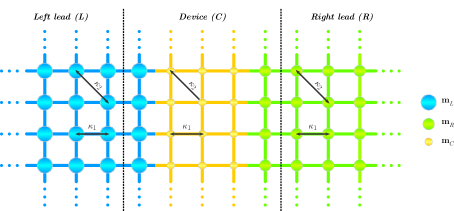
Figure 2: A schematic representation the system consisting of a square lattice with the same lattice constant and force constants ($\kappa_{1}$ for first-neighbor and $\kappa_{2}$ for second-neighbor) throughout. The masses are different in the three regions: they are $m_{L}$ in the left lead, $m_{C}$ in the central region, and $m_{R}$ in the right lead.

	$\omega=1.55$	$\omega=2.20$
$\triangle\mathbf{g}_{L}$	$\left[\begin{array}[]{cc}2.1156&8.4644\\ 8.4688&30.4458\end{array}\right]$$10^{-12}$	$\left[\begin{array}[]{cc}2.1717&0.7383\\ 0.7402&0.3862\end{array}\right]$$10^{-12}$
$\triangle\mathbf{g}_{R}$	$\left[\begin{array}[]{cc}0.9315&3.2897\\ 3.2895&12.0360\end{array}\right]$$10^{-12}$	$\left[\begin{array}[]{cc}0.7092&0.9069\\ 0.9066&2.3428\end{array}\right]$$10^{-12}$
$\triangle\mathbf{B}_{L}$	$\left[\begin{array}[]{cc}2.0924&3.0534\\ 8.9079&11.0897\end{array}\right]$$10^{-12}$	$\left[\begin{array}[]{cc}2.5303&1.0733\\ 1.1024&0.2075\end{array}\right]$$10^{-12}$
$\triangle\mathbf{B}_{R}$	$\left[\begin{array}[]{cc}2.3381&1.8484\\ 7.8625&6.8557\end{array}\right]$$10^{-12}$	$\left[\begin{array}[]{cc}1.5516&0.6837\\ 2.4664&1.2571\end{array}\right]$$10^{-12}$
$\triangle\boldsymbol{\Gamma}_{L}$	$\left[\begin{array}[]{cc}3.0993&6.0824\\ 6.0837&3.0986\end{array}\right]$$10^{-12}$	$\left[\begin{array}[]{cc}3.3946&2.0217\\ 2.0255&0.8398\end{array}\right]$$10^{-12}$
$\triangle\boldsymbol{\Gamma}_{R}$	$\left[\begin{array}[]{cc}3.1228&9.1446\\ 9.1450&3.1148\end{array}\right]$$10^{-12}$	$\left[\begin{array}[]{cc}5.1781&3.0598\\ 3.0615&0.6453\end{array}\right]$$10^{-12}$
$\triangle\mathbf{V}_{L}^{a}$	$\left[\begin{array}[]{cc}3.0985&5.1429\\ 5.1422&3.1002\end{array}\right]$$10^{-12}$	$\left[\begin{array}[]{cc}0.2061&0.5931\\ 0.5897&3.2494\end{array}\right]$$10^{-12}$
$\triangle\mathbf{V}_{R}$	$\left[\begin{array}[]{cc}3.1173&6.5236\\ 6.5243&3.1151\end{array}\right]$$10^{-12}$	$\left[\begin{array}[]{cc}1.6979&1.6577\\ 1.6571&3.1965\end{array}\right]$$10^{-12}$
$\triangle T$	$7.9869\times 10^{-12}$	$0.7000\times 10^{-12}$

Table 2: The absolute value of the differences between various quantities computed using the WFM and the AGF formalisms for $k_{y}=1$. The quantities are the left ($\mathbf{g}_{L}$) and right ($\mathbf{g}_{R}$) surface Green’s functions, the left ($\mathbf{B}_{L}$) and right ($\mathbf{B}_{R}$) Bloch matrices, the left ($\boldsymbol{\Gamma}_{L}$) and right ($\boldsymbol{\Gamma}_{R}$) escape rates and the transmission $T$. In the AGF formalism we used $\eta=10^{{}^{-12}}$.

	$\mathbf{Q}_{inj}$	$\mathbf{Q}_{inj}^{K}$
$\omega=0.50$	$\left[\begin{array}[]{cc}0&0\\ 0&0\end{array}\right]$	$\left[\begin{array}[]{cc}-0.7730-0.0022i&-0.0017-0.5730i\\ -0.0018+0.6537i&-1.0162+0.0030i\end{array}\right]$
$\omega=1.00$	$\left[\begin{array}[]{cc}-0.0072-1.1453i&-0.0000-0.0000i\\ -0.6058+0.0038i&0.0000+0.0000i\end{array}\right]$	$\left[\begin{array}[]{cc}-0.9992-0.5597i&-0.4055-0.6913i\\ -0.2960+0.5285i&-0.3641-0.6208i\end{array}\right]$
$\omega=1.55$	$\left[\begin{array}[]{cc}0.2629-0.1315i&-2.0993+0.8788i\\ -0.2748+0.1374i&-0.1968+0.0824i\end{array}\right]$	$\left[\begin{array}[]{cc}0.2914-0.0385i&-1.2456-1.9046i\\ -0.3046+0.0403i&-0.1168-0.1785i\end{array}\right]$
$\omega=2.20$	$\left[\begin{array}[]{cc}-0.0000-0.0000i&-1.4994-0.5448i\\ -0.0000-0.0000i&-0.2194+0.6038i\end{array}\right]$	$\left[\begin{array}[]{cc}0.6107+0.0604i&1.5771-0.2403i\\ -2.4851-0.2459i&-0.0968-0.6351i\end{array}\right]$

Table 3: The injection matrices computed with our WFM method($\mathbf{Q}_{inj}$) and with the method used in Komyakov et al. [2] ($\mathbf{Q}_{inj}^{K}$), for $k_{y}=1$. We consider three frequencies:$\omega=0.50$, $\omega=1.00$, $\omega=1.55$ and $\omega=2.20$.

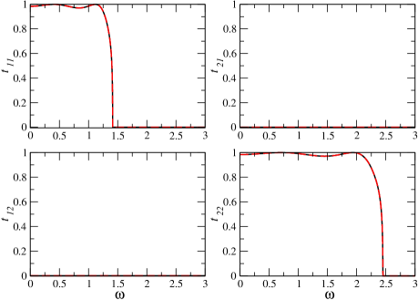
Figure 3: Mode-resolved transmission amplitudes for $k_{y}=0$. Our results are shown in black continued line, and the results obtained using the Fisher-Lee formula are shown in red dashed line.

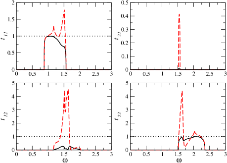
Figure 4: Mode-resolved transmission amplitudes for $k_{y}=1$. Our results are shown in black continued line, and the results obtained using the Fisher-Lee formula are shown in red dashed line. Where relevant a horizontal dotted line is added to mark the maximum allowed value of unity for the transmission amplitude.

4 Applications

In this part, we demonstrate the strength of our method by illustrating its application with a simple model, and also by comparing it to previous common methods. We consider the case of the 2D square lattice, of lattice constant $a$, with the central part made up of three atomic planes as shown in Fig 2. The force constants are identical throughout the system, but we choose to use a different mass for each part of the device. The force constants are $\kappa_{1}$ and $\kappa_{2}=0.5\;\kappa_{1}$ for the first and second-neighbor interactions, respectively. The masses are $m_{L}$ for the left lead, $m_{R}=0.6\;m_{L}$ for the right lead, and $m_{C}=0.8\;m_{L}$ for the central part. We define the frequency unit $\omega_{0}=\sqrt{\kappa_{1}/m_{L}}$. Henceforth the frequency $\omega$ is given in units of $\omega_{0}$.

In Table 2 we report the differences between various quantities computed both with our WFM method and with the AGF method for a wave vector $k_{y}=1$ and for two frequencies: $\omega=1.55$ and $\omega=2.20$. The latter are chosen so as to include both propagating and evanescent or decaying modes. In the AGF method we chose the parameter $\eta=10^{-12}$. In theory the parameter $\eta$ is infinitesimal and one is to take the limit $\eta\to 0^{+}$ to recover the correct result. In the current calculation, however, we have no access to a closed-form final formula, and if a limit is to be taken, it has to be numerical in nature. Our choice of a fixed value is only meant to serve as an illustration. It is clear from Table 2 that indeed all the relevant quantities agree perfectly when computed with either of the methods. The differences are, indeed, due only to the size of the parameter $\eta$. This is a clear demonstration of the complete equivalence of our WFM method and the AGF method as shown above.

In Table 3 we report the values of the injection matrix computed both with our WFM method ($\mathbf{Q}_{inj}$) and with the “classical” WFM by Komyakov et al.[2] ($\mathbf{Q}_{inj}^{K}$) for the wave vector $k_{y}=1$. We considered four frequencies: $\omega=0.50$, $\omega=1.00$, $\omega=1.55$ and $\omega=2.20$. These are chosen so as to include both propagating and evanescent modes. It is clear that, whenever one or both of the modes are decaying, our method yields a vanishing matrix element corresponding to the transmission from that mode. However, the classical method always gives finite matrix elements. As a result, our method selects from the outset only the transmission from a propagating mode. In the classical method this is not the case, and to obtain the final transmission amplitudes one has to zero out by hand the transmission amplitude whenever “incoming” mode is decaying.

We show in Fig. 3 the mode-resolved transmission amplitudes for the case of $k_{y}=0$ as obtained by our method and as obtained using the Fisher-Lee formula. It is evident that our results coincide perfectly with those from the Fisher-Lee formula. In Fig. 4 we show the same quantities computed for $k_{y}=1$. We now can see that the results are very different than one another. Moreover, it is striking to see that the transmission amplitudes computed using the Fisher-Lee relation are in some cases greater than the maximum allowed value of unity. The difference, as discussed above, appears only when the wave vector matrices $\mathbf{C}_{L}^{a}$ and $\mathbf{C}_{R}$ are not orthogonal. This is, indeed, the case for the choice $k_{y}=1$. We surmise that the failure of the Fisher-Lee relation to give proper mode-resolved transmission amplitudes has eluded researchers because they probably checked their results only in the particular situations where the wave vector matrices are orthogonal; this is the case when $k_{y}=0$ as shown above. And, more importantly, many such applications were carried out in the one-dimensional case where such situation is never encountered.

5 Conclusion

In conclusion, we have reformulated the conventional WFM method and completed its equivalence with the AGF approach. Through a clever choice of the evanescent eigenmodes entering the calculation, we need only use four Bloch matrices, getting rid of the redundant four others introduced in earlier literature, and which have no counterparts in the AGF method. This choice also means that the injection matrix selects from the outset the propagating modes as the sole that contribute to the transmission. In order to arrive at the equivalence, we showed how to obtain the group velocity matrices used in the WFM method from the “escape rates” defined in the AGF formalism. This then allowed us to proceed to a more physical spectral decomposition of the transmission amplitude. The “escape rates” are related to the self-energies, and these are computed differently in the WFM and in the AGF formalisms. In the first, they are obtained from the Bloch matrices, and in the second from the surface Green’s functions of the leads. The findings of this study intimate that when proper care is taken in the choice of the phonon modes that enter the machinery of the WFM method, its equivalence with the AGF technique is complete. As an illustration, we applied our method to a simple model and, additionally, we made a thorough comparison with earlier methods. Our results demonstrate the equivalence of the two methods to a very high accuracy, limited only by the machine precision. The comparison with the Fisher-Lee relation sheds a light on its failure to properly decompose the transmission into individual contributions of the phonon modes.

We have succeeded in completing the equivalence of the two most widely used methods in ballistic transport at the nanoscale. Besides, we have devised a procedure that provides a number of advantages when compared to earlier approaches. The main advantages of our method are as follows:

1. We used the inverse of the Bloch factor in the eigenvalue problem of the left lead, conventionally chosen as the side from which the incident phonons arrive. This choice precludes many costly matrix inversions in the following steps of the procedure.

2. We defined four Bloch matrices, instead of eight as in Refs. [2, 32], which are enough to carry out all the subsequent calculations.

3. Our injection matrix selects out the evanescent modes from the outset. In prior methods [2]. the latter are eliminated “by hand” or by using a projector operator to project out their unwanted contribution (Eq. 2.62 in [2]).

4. Each of the four Bloch matrices defined in this work has its equivalent quantity in the AGF method, contrary to the eight matrices defined in prior methods, where four of them have no corresponding quantities in the AGF method.

5. The transmission function in our method is given in terms of the bulk group velocities of the leads. These are guaranteed to be diagonal and positive, and their square roots are clearly defined. However, in prior methods, the transmission function is written in terms of the “escape rates”. These being defined as the difference between a self-energy matrix and its conjugate, are not necessarily real as is assumed in most publications [17, 45, 44, 46].

6. And of utmost importance, we derived a generalized Fisher-Lee formula to properly decompose the transmission function into individual phonon mode contributions, which is valid regardless of the orthogonality of the eigenvectors.

These findings add to a growing body of literature on the theoretical investigation of transport, thermal as well as electronic, through interfaces at the nanoscale. The complete equivalence of the two most widely used methods allows for a better understanding of the underlying physics, especially in the AGF method, where, despite its obvious mathematical superiority, lacks somewhat the transparency inherent to the WFM method.

Appendix A Velocity matrices

Starting from the definition of the Bloch matrix $\mathbf{B}_{R}=\mathbf{C}_{R}\boldsymbol{\Lambda}_{R}\tilde{\mathbf{C}}_{R}$, we have $\mathbf{B}_{R}\mathbf{C}_{R}=\mathbf{C}_{R}\boldsymbol{\Lambda}_{R}$ and $\mathbf{C}_{R}^{\dagger}\mathbf{B}_{R}^{\dagger}=\boldsymbol{\Lambda}_{R}^{\dagger}\mathbf{C}_{R}^{\dagger}$. We make use of these equalities in the definition of the velocity matrix (Eq. 16) and obtain

$$\mathbf{V}_{R}= \mathrm{i}\left[\mathbf{C}_{R}^{\dagger}\,\mathbf{H}_{RR}\,\mathbf{C}_{R}\,\mathbf{\boldsymbol{\Lambda}}_{R}-\mathbf{\boldsymbol{\Lambda}}_{R}^{\dagger}\,\mathbf{C}_{R}^{\dagger}\,\mathbf{H}_{RR}^{\dagger}\,\mathbf{C}_{R}\right]$$

$$= \mathrm{i}\left[\mathbf{C}_{R}^{\dagger}\,\mathbf{H}_{RR}\,\mathbf{B}_{R}\,\mathbf{C}_{R}-\mathbf{C}_{R}^{\dagger}\,\mathbf{B}_{R}^{\dagger}\,\mathbf{H}_{RR}^{\dagger}\,\mathbf{C}_{R}\right]$$

$$= \mathrm{i}\,\mathbf{C}_{R}^{\dagger}\left[\mathbf{H}_{RR}\,\mathbf{B}_{R}-\mathbf{B}_{R}^{\dagger}\,\mathbf{H}_{RR}^{\dagger}\right]\mathbf{C}_{R}$$

$$= \mathrm{i}\,\mathbf{C}_{R}^{\dagger}\left[\mathbf{\boldsymbol{\Sigma}}_{R}-\mathbf{\boldsymbol{\Sigma}}_{R}^{\dagger}\right]\mathbf{C}_{R}$$

$$= \mathrm{i}\,\mathbf{C}_{R}^{\dagger}\left[\mathbf{\boldsymbol{\Sigma}}_{R}-\mathbf{\boldsymbol{\Sigma}}_{R}^{a}\right]\mathbf{C}_{R}$$

$$= \mathbf{C}_{R}^{\dagger}\,\mathbf{\boldsymbol{\Gamma}}_{R}\,\mathbf{C}_{R},$$ (68)

where we used the expressions of the self-energy matrices in terms of the Bloch matrices as given in Eq. 35.

Starting again from the definition of the Bloch matrix $\mathbf{B}_{L}^{a}=\mathbf{C}_{L}^{a}\boldsymbol{\Lambda}_{L}^{a}\tilde{\mathbf{C}}_{L}^{a}$, we have $\mathbf{B}_{L}^{a}\mathbf{C}_{L}^{a}=\mathbf{C}_{L}^{a}\boldsymbol{\Lambda}_{L}^{a}$ and $\mathbf{C}_{L}^{a\dagger}\mathbf{B}_{L}^{a\dagger}=\boldsymbol{\Lambda}_{L}^{a\dagger}\mathbf{C}_{L}^{a\dagger}$. Similarly, we make use of these equalities in the definition of the velocity matrix (Eq. 19) and obtain

$$\mathbf{V}_{L}^{a}= -\mathrm{i}\left[\mathbf{C}_{L}^{a\dagger}\,\mathbf{H}_{LL}^{\dagger}\,\mathbf{C}_{L}^{a}\,\mathbf{\boldsymbol{\Lambda}}_{L}^{a}-\mathbf{\boldsymbol{\Lambda}}_{L}^{a\dagger}\,\mathbf{C}_{L}^{a\dagger}\,\mathbf{H}_{LL}\,\mathbf{C}_{L}^{a}\right]$$

$$= -\mathrm{i}\left[\mathbf{C}_{L}^{a\dagger}\,\mathbf{H}_{LL}^{\dagger}\,\mathbf{B}_{L}^{a}\,\mathbf{C}_{L}^{a}-\mathbf{C}_{L}^{a\dagger}\,\mathbf{B}_{L}^{a\dagger}\,\mathbf{H}_{LL}\,\mathbf{C}_{L}^{a}\right]$$

$$= -\mathrm{i}\,\mathbf{C}_{L}^{a\dagger}\left[\mathbf{H}_{LL}^{\dagger}\,\mathbf{B}_{L}^{a}-\mathbf{B}_{L}^{a\dagger}\,\mathbf{H}_{LL}\right]\mathbf{C}_{L}^{a}$$

$$= -\mathrm{i}\,\mathbf{C}_{L}^{a\dagger}\left[\mathbf{\boldsymbol{\Sigma}}_{L}^{a}-\mathbf{\boldsymbol{\Sigma}}_{L}^{a\dagger}\right]\mathbf{C}_{L}^{a}$$

$$= -\mathrm{i}\,\mathbf{C}_{L}^{a\dagger}\left[\mathbf{\boldsymbol{\Sigma}}_{L}^{a}-\mathbf{\boldsymbol{\Sigma}}_{L}\right]\mathbf{C}_{L}^{a}$$

$$= \mathbf{C}_{L}^{a\dagger}\mathbf{\boldsymbol{\Gamma}}_{L}\,\mathbf{C}_{L}^{a},$$ (69)

where we used the expressions of the self-energy matrices in terms of the Bloch matrices as given in Eq. 51.

Appendix B Injection matrix

From Eq. 40, we have $\mathbf{Q}_{\mathrm{inj}}=\mathbf{H}_{LL}^{\dagger}(\mathbf{B}_{L}^{a}-\mathbf{B}_{L})\mathbf{C}_{L}^{a}$ and from Eqs. 36 and 51, we have

$$\mathbf{Q}_{\mathrm{inj}}=(\boldsymbol{\Sigma}_{L}^{a}-\boldsymbol{\Sigma}_{L})\mathbf{C}_{L}^{a}=i\boldsymbol{\Gamma}_{L}\mathbf{C}_{L}^{a}.$$ (70)

Then, from Eq. 60, the injection matrix reads

$$\mathbf{Q}_{\mathrm{inj}}=i\left(\mathbf{C}_{L}^{a\dagger}\right)^{-1}\mathbf{V}_{L}^{a}.$$

Appendix C Eigenvector matrices from the Green’s functions

From Eqs. 29 and 32, we multiply by $\mathbf{C}_{L}^{a}$ and $\mathbf{C}_{R}$ on the right and obtain

$$\mathbf{B}_{L}^{a}\mathbf{C}_{L}^{a}=\mathbf{C}_{L}^{a}\boldsymbol{\Lambda}_{L}^{a}$$

and

$$\mathbf{B}_{R}\mathbf{C}_{R}=\mathbf{C}_{R}\boldsymbol{\Lambda}_{R}.$$

Also from the expressions of $\mathbf{B}_{L}^{a}$ and $\mathbf{B}_{R}$in terms of the surface Green’s functions(Eqs. 46 and 55), we obtain the following right eigenvalue equation for the eigenvector matrices $\mathbf{C}_{L}^{a}$ and $\mathbf{C}_{R}$:

$$\begin{array}[]{ccc}\mathbf{g}_{L}^{a}\mathbf{H}_{LL}\mathbf{C}_{L}^{a}&=&\mathbf{C}_{L}^{a}\boldsymbol{\Lambda}_{L}^{a},\\ \mathbf{g}_{R}\mathbf{H}_{RR}^{\dagger}\mathbf{C}_{R}&=&\mathbf{C}_{R}\boldsymbol{\Lambda}_{R}.\end{array}$$

These are similar to the expressions found by Ong [32].

References

• [1] Ando T 1991 Phys. Rev. B 44 8017.
• [2] Khomyakov P A , Brocks G, Karpan V, Zwierzycki M and Kelly P J 2005 Phys. Rev. B 72 035450.
• [3] Datta S 1997 Electronic Transport in Mesoscopic Systems (Cambridge University Press).
• [4] Di Ventra M 2008 Electrical Transport in Nanoscale Systems (Cambridge University Press).
• [5] Evers F, Korytár R, Tewari S and van Ruitenbeek J M Advances and challenges in single-molecule electron transport, arXiv:1906.10449 [cond-mat.mes-hall].
• [6] Bell L E 2008 Science 321 1457.
• [7] Dubi Y and Di Ventra M 2011 Rev. Mod. Phys. 83 131.
• [8] Cahill D G, Braun P V, Chen G, Clarke D R, Fan S, Goodson K E, Keblinski P, King W P, Mahan G D, Majumdar A, Maris H J, Phillpot S R, Pop E and Shi L 2014 Appl. Phys. Rev. 1 011305.
• [9] Freericks J K 2006 Transport in multilayered nanostructures: the dynamical mean-field theory approach (Imperial College Press, London).
• [10] Landauer R 1957 IBM J. Res. Dev. 1 233.
• [11] Landauer R 1970 Philos. Mag. 21 863.
• [12] Khomyakov P A and Brocks G 2004 Phys. Rev. B 70 195402.
• [13] Xia K, Zwierzycki M, Talanana M, Kelly P J and Bauer G E W 2006 Phys. Rev. B 73 064420.
• [14] Farmanbar M, Amlaki T and Brocks G, 2016 Phys. Rev.93 205444.
• [15] Chen X, Xu Y, Wang J and Guo H, 2019 Phys. Rev. B 99 064302.
• [16] Mingo N and Yang L 2003 Phys. Rev. B 68 245406.
• [17] Wang J S, Wang J and Lü J T 2008 Eur. Phys. J. B 62 381.
• [18] Zhang W, Fisher T and Mingo N 2007 ASME J. Heat Transfer 129 483.
• [19] Li X and Yang R 2012 Phys. Rev. B 86 054305.
• [20] Gu X, Li X and Yang R 2015 Phys. Rev. B 91 205313.
• [21] Tian Z, Esfarjani K and Chen G 2012 Phys. Rev. B 86 235304.
• [22] Caroli C, Combescot R, Nozieres P and Saint-James D 1971 J. Phys. C 4 916.
• [23] Keldysh L V 1965 Sov. Phys. JETP 20 1018.
• [24] Zhu Y and Liu L 2016 Atomistic Simulation of Quantum Transport in Nanoelectronic Devices (World Scientific, Singapore).
• [25] Krstić P S, Zhang X G and Butler W H 2002 Phys. Rev. B 66 205319
• [26] Giannozzi P, Baroni S, Bonini N, et al., J.Phys.:Condens.Matter 21, 395502 (2009); Giannozzi P, Andreussi O, Brumme T, et al., J.Phys.:Condens.Matter 29, 465901 (2017)
• [27] H. Ebert, D. Ködderitzsch, and J. Minár, Rep. Prog. Phys. 74, 096501 (2011).
• [28] Huang Z, Murthy J Y and Fisher T S 2011 J. Heat Transfer 133 114502.
• [29] Sadasivam S, Waghmare U V and Fisher T S 2017 Phys. Rev. B 96 174302.
• [30] Ong Z Y and Zhang G 2015 Phys. Rev. B 91 174302.
• [31] Latour B, Shulumba N and Minnich A J 2017 Phys. Rev. B 96 104310.
• [32] Ong Z Y 2018 J. Appl. Phys. 124 151101.
• [33] Klöckner J C, Cuevas J C and Pauly F 2018 Phys. Rev. B 97 155432.
• [34] Fisher D S and Lee P A 1981 Phys. Rev. B 23 6851.
• [35] Ferry D K and Goodnick S M 2001 Transport in Nanostructures (Cambridge University Press).
• [36] Sanvito S, Lambert C J, Jefferson J H and Bratkovsky A M 1999 Phys. Rev. B 59 11936.
• [37] Wimmer M 2009 Quantum transport in nanostructures: From computational concepts to spintronics in graphene and magnetic tunnel junctions PhD Thesis Regensburg University.
• [38] Zhang S H, Yang W and Chang K 2017 Phys. Rev. B 95 075421.
• [39] Cohen-Tannoudji C, Diu B and Lalöe F 1977 Quantum Mechanics (John Wiley & Sons, New York).
• [40] Mingo N 2009 Green’s function methods for phonon transport through nano-contacts (Springer, Heidelberg).
• [41] Sadasivam S, Che Y, Huang Z, Chen L, Kumar S and Fisher T S 2014 Annu. Rev. Heat Transfer 17 89.
• [42] Lopez Sancho M P, Lopez Sancho J M and Rubio J 1985 J. Phys. F: Met. Phys. 15 851.
• [43] Velev J and Butler W 2004 J. Phys.: Condens. Matter 16 R637
• [44] Cuevas J C and Scheer E 2017 Molecular Electronics: An Introduction to Theory and Experiment (World Scientic, Singapore, 2nd edition edition).
• [45] Cuevas J C, Yeyati A L and Martín-Rodero A, 1998 Phys. Rev. Lett. 80 1066.
• [46] Häfner M, Viljas J K, Frustaglia D, Pauly F, Dreher M, Nielaba P and Cuevas J C 2008 Phys. Rev. B 77 104409.