Wigner Crystallization of Electrons in a One-Dimensional Lattice:
A Condensation in the Space of States

Abstract

We study the ground state of a system of spinless electrons interacting through a screened Coulomb potential in a lattice ring. By using analytical arguments, we show that, when the effective interaction compares with the kinetic energy, the system forms a Wigner crystal undergoing a first-order quantum phase transition. This transition is a condensation in the space of the states and belongs to the class of quantum phase transitions discussed in J. Phys. A 54, 055005 (2021). The transition takes place at a critical value ${r_{s}}_{c}$ of the usual dimensionless parameter $r_{s}$ (radius of the volume available to each electron divided by effective Bohr radius) for which we are able to provide rigorous lower and upper bounds. For large screening length these bounds can be expressed in a closed analytical form. Demanding Monte Carlo simulations allow to estimate ${r_{s}}_{c}\simeq 2.3\pm 0.2$ at lattice filling $3/10$ and screening length 10 lattice constants. This value is well within the rigorous bounds $0.7\leq{r_{s}}_{c}\leq 4.3$. Finally, we show that if screening is removed after the thermodynamic limit has been taken, ${r_{s}}_{c}$ tends to zero. In contrast, in a bare unscreened Coulomb potential, Wigner crystallization always takes place as a smooth crossover, not as a quantum phase transition.

The Wigner crystal (WC) Wigner , namely, the periodic arrangement of electrons that minimizes the Coulomb interaction energy in the presence of band motion effects Hubbard1978 , has been investigated in several long-range repulsive potential models Sinai1983 ; Bak1982 ; Fratini2004 ; Slavin2005 . Two dimensional 2DEG_1989 ; 2DEG_1996 ; 2DEG_2002 ; 2DEG_2009 ; 2DEG_2017 ; Noda2002 and one-dimensional Siegmund2009 ; VFB2003 electron gases at zero temperature have been extensively studied from a theoretical point of view. A recent experiment succeeded in imaging an electronic WC in one-dimensional nanotubes nanotube .

The occurrence of a WC is often argued by comparing the typical kinetic and Coulomb energies involved. Roughly speaking, the kinetic energy can be evaluated as $\hbar^{2}/(2m^{*}r^{2})$, where $m^{*}$ is the effective electron mass and $r$ the radius of the volume available to each electron, whereas the Coulomb energy can be taken as $e^{2}/r$, where $e$ is the electron charge. These two energies have the same value when $r_{s}\equiv r/a_{B}$, $a_{B}$ being the effective Bohr radius, is equal to the “critical value” ${r_{s}}_{c}=2$. Then one concludes that for $r_{s}>{r_{s}}_{c}$ a WC must show up.

The above argument can be, however, misleading. Consider the case of the unscreened Coulomb potential in a $d$-dimensional space with a fixed value of $r_{s}$. For a gas of $N_{p}$ electrons, the energy per particle of the bare $d$-dimensional Coulomb potential scales as ${N_{p}}^{d-1}$ for $d>1$, and as $\ln N_{p}$ for $d=1$ Dubin . On the other hand, at any dimension $d$, the kinetic energy per particle is independent of $N_{p}$, so that the potential energy overwhelms the kinetic one for $N_{p}$ large enough. In other words: in the thermodynamic limit ($\operatorname{TD-lim}$), ${r_{s}}_{c}\to 0^{+}$ and no quantum phase transition (QPT) takes place, the system being trivially a WC for any $r_{s}>0$; for finite $N_{p}$, instead, the transition from free electron motion to WC obtained by increasing $r_{s}$ is just a smooth crossover, not a QPT.

Screening is, therefore, an essential ingredient Hubbard1978 : the ground-state (GS) energy per particle of the screened potential scales linearly with $N_{p}$ and can fairly compete with the kinetic term. It is only in this case that we can hope to observe a QPT in the $\operatorname{TD-lim}$ by varying $r_{s}$.

We are not aware of any conclusive study on the phase transition nature of the Wigner crystallization, except for the work of Brascamp and Lieb on the $1d$ plasma in a neutralizing background Lieb2002 . Here, we study the ground state of a system of spinless electrons interacting through a screened $3d$ Coulomb potential in a lattice ring. By using analytical arguments, we demonstrate that, for any finite screening length, the Wigner crystallization is a QPT taking place at a finite critical value ${r_{s}}_{c}$ of the parameter $r_{s}$. For ${r_{s}}_{c}$ we provide rigorous upper and lower bounds, which can be cast in an analytical form in the limit of large screening length. The QPT that we find is of first order (according to Ehrenfest classification) and falls within the class of condensations in the space of states introduced in QPT . Demanding Monte Carlo (MC) simulations based on an advanced bias-free code MC allow to estimate a value of ${r_{s}}_{c}$, which is well within the rigorous bounds. Finally, we show that, removing the screening after the $\operatorname{TD-lim}$ has been taken, we have ${r_{s}}_{c}\to 0^{+}$, confirming that a nonzero minimal screening is necessary to have a realistic physical picture.

We briefly recall the mechanism of first-order QPT of QPT . To be specific, let us consider a lattice model with $N$ sites and $N_{p}$ particles described by a Hamiltonian

$$H=K+gV,$$ (1)

where $K$ and $V$ are Hermitian noncommuting operators, and $g$ a free dimensionless parameter, which, without loss of generality, can be taken to be non-negative. Regardless of the details of $K$ and $V$, we represent $H$ in the eigenbasis of $V$ and it is natural to call $V$ the potential operator, and $K$ the hopping operator. To exclude trivial behaviors, we suppose that the eigenvalues of $K$ and $V$ scale linearly with the number of particles $N_{p}$. Since in the two opposite limits $g\to 0$ and $g\to\infty$, the GS of the system tends to the GS of $K$ and $V$, respectively, we wonder if, in the $\operatorname{TD-lim}$, this transition occurs as a QPT taking place at some critical value $g_{c}$.

A quite general kind of QPT is the condensation in the space of states. We decompose the Hilbert space $\mathbb{F}$ of the system as the direct sum of two mutually orthogonal subspaces, denoted condensed and normal, namely, $\mathbb{F}=\mathbb{F}_{\mathrm{cond}}\oplus\mathbb{F}_{\mathrm{norm}}$. The definition of these subspaces is as follows. We write $\mathbb{F}=\mathrm{span}\{|n\rangle\}_{n=1}^{M}$, where $\{|n\rangle\}$ (later on called configurations) is a complete orthonormal set of eigenstates of $V$, i.e., we have $V|n\rangle=V_{n}|n\rangle$, $n=1,\dots,M$, where we assume ordered, possibly degenerate, potential values $V_{1}\leq V_{2}\leq\dots\leq V_{M}$. Given an integer $M_{\mathrm{cond}}<M$, we then define $\mathbb{F}_{\mathrm{cond}}=\mathrm{span}\{|n\rangle\}_{n=1}^{M_{\mathrm{cond}}}$ and $\mathbb{F}_{\mathrm{norm}}=\mathrm{span}\{|n\rangle\}_{n=M_{\mathrm{cond}}+1}^{M}=\mathbb{F}_{\mathrm{cond}}^{\perp}$. This definition essentially relies on the choice of the dimension $M_{\mathrm{cond}}$, which, in view of the ordering of the potential values, marks the maximum potential value included in the condensed subspace

$$\max V_{\mathrm{cond}}=\max\{V_{n}:\leavevmode\nobreak\ |n\rangle\in\mathbb{F}_{\mathrm{cond}}\}=V_{M_{\mathrm{cond}}}.$$ (2)

Consider the GS energies of the system, the condensed, and normal subspaces:

$$E =\inf_{|u\rangle\in\mathbb{F}}\langle u|H|u\rangle/\langle u|u\rangle,$$ (3)

$$E_{\mathrm{cond}} =\inf_{|u\rangle\in\mathbb{F}_{\mathrm{cond}}}\langle u|H|u\rangle/\langle u|u\rangle,$$ (4)

$$E_{\mathrm{norm}} =\inf_{|u\rangle\in\mathbb{F}_{\mathrm{norm}}}\langle u|H|u\rangle/\langle u|u\rangle.$$ (5)

We are interested in the situations where $M_{\mathrm{cond}}/M\ll 1$ and, as a consequence, $M_{\mathrm{norm}}/M\equiv(M-M_{\mathrm{cond}})/M\simeq 1$. This justifies the names condensed and normal assigned to the two subspaces and suggests the following dichotomy argument: since $\mathbb{F}\simeq\mathbb{F}_{\mathrm{norm}}$, we have $E\simeq E_{\mathrm{norm}}$—unless—it is energetically more convenient to “freeze” into the infinitely smaller subspace $\mathbb{F}_{\mathrm{cond}}$, where we get $E\simeq E_{\mathrm{cond}}$.

The above heuristic argument can be cast in rigorous terms as follows. The $\operatorname{TD-lim}$ is defined as the limit $N,N_{p}\to\infty$ with $N_{p}/N=\varrho$ constant. Consider the rescaled energies:

$$\epsilon(g) =\operatorname{TD-lim}E(N,N_{p},g)/N_{p},$$ (6)

$$\epsilon_{\mathrm{cond}}(g) =\operatorname{TD-lim}E_{\mathrm{cond}}(N,N_{p},g)/N_{p},$$ (7)

$$\epsilon_{\mathrm{norm}}(g) =\operatorname{TD-lim}E_{\mathrm{norm}}(N,N_{p},g)/N_{p},$$ (8)

which are finite in view of the assumed scaling properties of $K$ and $V$ (dependence on $\varrho$ is left understood). In QPT we have proved the following general theorem

$$\mbox{if}\leavevmode\nobreak\ \operatorname{TD-lim}{M_{\mathrm{cond}}/M}=0,$$ (9a)

$$\mbox{then}\leavevmode\nobreak\ \epsilon=\min\{\epsilon_{\mathrm{cond}},\epsilon_{\mathrm{norm}}\}.$$ (9b)

This theorem establishes the possibility of a QPT between a normal phase characterized by the energy per particle $\epsilon_{\mathrm{norm}}$, obtained by removing from $\mathbb{F}$ the infinitely smaller subspace $\mathbb{F}_{\mathrm{cond}}$, and a condensed phase characterized by the energy per particle $\epsilon_{\mathrm{cond}}$, obtained by restricting the action of $H$ onto $\mathbb{F}_{\mathrm{cond}}$. The situation is particularly simple for systems characterized by a single parameter as in the case of Eq. (1). If Eq. (9a) holds and, moreover, the functions $\epsilon_{\mathrm{norm}}(g)$ and $\epsilon_{\mathrm{cond}}(g)$ are such that the equation

$$\epsilon_{\mathrm{norm}}(g)=\epsilon_{\mathrm{cond}}(g)$$ (10)

admits a unique finite solution $g=g_{c}$, Eq. (9b) provides

$$\epsilon(g)=\left\{\begin{array}[]{ll}\epsilon_{\mathrm{norm}}(g),&g<g_{c},\\ \epsilon_{\mathrm{cond}}(g),&g>g_{c}.\end{array}\right.$$ (13)

Equations (10) and (13) imply the existence of a first-order QPT at the critical point $g_{c}$. In fact, although in general $\epsilon_{\mathrm{cond}}(g)$ and $\epsilon_{\mathrm{norm}}(g)$ are separately analytic in $g=g_{c}$, on observing that $\epsilon_{\mathrm{cond}}(g)$ and $\epsilon_{\mathrm{norm}}(g)$ are different functions, we conclude that, while $\epsilon(g)$ is continuous at $g=g_{c}$, its first derivative undergoes the discontinuity $|\epsilon_{\mathrm{cond}}^{\prime}(g_{c})-\epsilon_{\mathrm{norm}}^{\prime}(g_{c})|>0$.

Whereas Eq. (9a) can be checked easily, the existence of a finite solution to Eq. (10) can be difficult to prove. A practical approach can be as follows. For $N,N_{p}$ finite with $N_{p}/N=\varrho$ constant, we evaluate $g_{\mathrm{cross}}(N,N_{p})$ as the value of the parameter $g$, if any, solution of the equation

$$E_{\mathrm{norm}}(N,N_{p},g)=E_{\mathrm{cond}}(N,N_{p},g).$$ (14)

Assuming a smooth limiting behavior, we expect

$$g_{c}=\operatorname{TD-lim}g_{\mathrm{cross}}(N,N_{p}).$$ (15)

Even if this limit cannot be exactly evaluated, as in the case of numerical simulations, Eq. (15) can be used to provide strict upper and lower bounds to $g_{c}$ as shown ahead.

To recapitulate, if we find a partition $\mathbb{F}=\mathbb{F}_{\mathrm{cond}}\oplus\mathbb{F}_{\mathrm{norm}}$ such that Eq. (9a) and Eq. (10) are satisfied, then a first-order QPT of the type introduced in QPT occurs at $g=g_{c}$. In general, such a partition is not unique. In fact, for Eq. (10) to admit a solution with condition (9a) satisfied, $\mathbb{F}_{\mathrm{cond}}$ can invariantly be chosen provided that it is not too small and not too large in such a way that neither of the two restrictions of $H$, to $\mathbb{F}_{\mathrm{cond}}$ and to $\mathbb{F}_{\mathrm{norm}}$, have a QPT. In this case, $\epsilon_{\mathrm{cond}}$ and $\epsilon_{\mathrm{norm}}$ are both analytic functions of $g$ at $g=g_{c}$, whereas $\epsilon$ is not. Note that, for finite sizes, different partitions of $\mathbb{F}$ lead, in general, to different values of both $E_{\mathrm{cond}}(g)$ and $E_{\mathrm{norm}}(g)$. Only in the $\operatorname{TD-lim}$ different invariant partitions of $\mathbb{F}$ lead to the same values of $\epsilon_{\mathrm{cond}}(g)$ for $g>g_{c}$ and $\epsilon_{\mathrm{norm}}(g)$ for $g<g_{c}$, namely, $\epsilon(g)$, as indicated by Eq. (13). We will exploit this invariance to get rigorous bounds to $g_{c}$.

We apply the above general strategy to a system of $N_{p}$ electrons interacting in a ring of $N$ sites. As usual, for simplicity and saving computational efforts, we consider spinless particles. The electronic Hamiltonian $H_{e}$ cast in the dimensionless form (1) by $H_{e}/t=H=K+gV$, $t=\hbar^{2}/(2m^{*}a^{2})$ being the hopping coefficient with $m^{*}$ the effective electron mass and $a$ the lattice constant VFB2003 , is given by

$$K =-\sum_{i=1}^{N}\left(c^{\dagger}_{i}c_{i+1}+c^{\dagger}_{i+1}c_{i}\right),$$ (16)

$$V =\sum_{i=1}^{N}\sum_{j=i+1}^{N}v_{i,j}c^{\dagger}_{i}c_{i}c^{\dagger}_{j}c_{j},$$ (17)

where the fermionic annihilation operators obey the periodic condition $c_{i+N}=c_{i}$. We consider a screened Coulomb interaction Hubbard1978

$$v_{i,j}=\frac{1}{d_{i,j}}e^{-ad_{i,j}/R},$$ (18)

$R$ being the screening length and $d_{i,j}=\min(j-i,N+i-j),\quad j>i$, the dimensionless distance between sites $i$ and $j$ in the ring. Screening takes into account the many-body effects not explicitly considered in $H$ and allows for the interaction energy to scale linearly with the number of particles $N_{p}$, as physically expected. The value of $R$ depends on the microscopic details of the system considered. However, whereas the minimum of $V$ has a logarithmic dependence on $R$, see later, the associated GS has a universal structure Hubbard1978 under conditions on $v_{i,j}$ Sinai1983 ; Bak1982 ; Slavin2005 that are fulfilled by Eq. (18) for any $R$. With the above choice for the potential, the dimensionless coupling $g$ in Eq. (1) takes the form of the following Seitz radius rs

$$g=2a/a_{B},\qquad a_{B}=\hbar^{2}/(m^{*}e^{2}).$$ (19)

Now we determine a partition $\mathbb{F}=\mathbb{F}_{\mathrm{cond}}\oplus\mathbb{F}_{\mathrm{norm}}$ which satisfies the conditions (9a) and (10). We recall that, according to Eq. (2), a partition is defined by specifying the maximum potential value allowed in $\mathbb{F}_{\mathrm{cond}}$.

As we show in SM , in the $\operatorname{TD-lim}$ the distribution of the potential values (17) divided by $N_{p}$ tends to a Dirac delta centered at $\overline{V}/N_{p}$, namely, the mean classical value of the potential per particle. This implies that, whenever $\max V_{\mathrm{cond}}/N_{p}<\overline{V}/N_{p}$, we have $M_{\mathrm{cond}}/M\to 0$ in the $\operatorname{TD-lim}$, i.e., Eq. (9a) is satisfied.

To comply with Eq. (10), consider that $E$, $E_{\mathrm{cond}}$, and $E_{\mathrm{norm}}$, are monotonously increasing functions of $g$ convex upward SM and suppose that the critical point is unique. It follows that $g_{c}$ is finite if and only if (i) $\epsilon_{\mathrm{norm}}(0)<\epsilon_{\mathrm{cond}}(0)$ and (ii) $\lim_{g\to\infty}\epsilon_{\mathrm{cond}}(g)/g<\lim_{g\to\infty}\epsilon_{\mathrm{norm}}(g)/g$.

Condition (i) is equivalent to saying that in the $\operatorname{TD-lim}$ $\min K_{\mathrm{norm}}/N_{p}<\min K_{\mathrm{cond}}/N_{p}$. Here and in the following, we use a notation as in Eq. (2), for example, $\min K_{\mathrm{cond}}$ is the smallest eigenvalue of the operator $K$ restricted to the condensed subspace, and so on. It’s easy to prove SM that, if Eq. (9a) is satisfied, the $\operatorname{TD-lim}$ of $\min K_{\mathrm{norm}}/\min K$ is 1, therefore, condition (i) is satisfied if in the $\operatorname{TD-lim}$ $\max V_{\mathrm{cond}}/N_{p}<\overline{V}/N_{p}$, i.e., $\max V_{\mathrm{cond}}\leq\overline{V}-\delta V$, with $\delta V>0$ being an arbitrary $O(N_{p})$ term.

Condition (ii) is equivalent to saying that in the $\operatorname{TD-lim}$ $\min V_{\mathrm{cond}}/N_{p}=\min V/N_{p}<\min V_{\mathrm{norm}}/N_{p}$. Since in the $\operatorname{TD-lim}$ we have $\min V_{\mathrm{norm}}/N_{p}=\max V_{\mathrm{cond}}/N_{p}$, the condition amounts to require $\max V_{\mathrm{cond}}/N_{p}>\min V/N_{p}$, i.e., $\max V_{\mathrm{cond}}\geq\min V+\delta V$, $\delta V>0$ being an arbitrary $O(N_{p})$ term.

In conclusion, the existence of any one of the partitions $\mathbb{F}=\mathbb{F}_{\mathrm{cond}}\oplus\mathbb{F}_{\mathrm{norm}}$ obtained choosing $\min V+O(N_{p})\leq\max V_{\mathrm{cond}}\leq\overline{V}-O(N_{p})$ allows us to say that, provided the screening length $R$ is finite, both Eqs. (9a) and (10) are satisfied. It follows that the Hamiltonian $H=K+gV$ of Eqs. (16-19) undergoes a Wigner crystallization in the form of a first-order QPT of the type introduced in QPT , i.e., as a condensation in the space of states. About the critical parameter $g_{c}$, at this level we just know that it is finite. The following of the Letter is devoted to the construction of upper and lower bounds of $g_{c}$ and, in order to do so, we shall exploit the invariance of the $\operatorname{TD-lim}$ (15) under different partitions of $\mathbb{F}$.

For finite $N$ and $N_{p}$, since $E_{\mathrm{cond}}$ and $E_{\mathrm{norm}}$ are monotonously increasing functions of $g$ convex upward, we have

$$g^{-}_{\mathrm{cross}}\leq g_{\mathrm{cross}}\leq g^{+}_{\mathrm{cross}},$$ (20)

where $g^{+}_{\mathrm{cross}}$ is the intersection point of two curves which are, respectively, a majorant of $E_{\mathrm{cond}}$ and a minorant of $E_{\mathrm{norm}}$, whereas $g^{-}_{\mathrm{cross}}$ is the intersection point of two curves which are, respectively, a minorant of $E_{\mathrm{cond}}$ and a majorant of $E_{\mathrm{norm}}$. Indicating with $g^{\pm}_{c}$ the $\operatorname{TD-lim}$s of $g^{\pm}_{\mathrm{cross}}$, we then have $g^{-}_{c}\leq g_{c}\leq g^{+}_{c}$. The more accurate are the approximations to $E_{\mathrm{cond}}$ and $E_{\mathrm{norm}}$, the tighter are the bounds $g^{\pm}_{c}$. However, we also want to choose these approximations to $E_{\mathrm{cond}}$ and $E_{\mathrm{norm}}$ sufficiently simple to allow for an analytical evaluation of the $\operatorname{TD-lim}$ of $g^{\pm}_{\mathrm{cross}}$.

Let us examine the following inequalities

$$E_{\mathrm{cond}}(g) \leq g\min V_{\mathrm{cond}},$$ (21)

$$E_{\mathrm{norm}}(g) \geq\min K_{\mathrm{norm}}+g\min V_{\mathrm{norm}},$$ (22)

and

$$E_{\mathrm{cond}}(g) \geq\min K_{\mathrm{cond}}+g\min V_{\mathrm{cond}},$$ (23)

$$E_{\mathrm{norm}}(g) \leq\min K_{\mathrm{norm}}+g\max V_{\mathrm{norm}}.$$ (24)

Equations (22), (23) and (24) are Weyl’s inequalities MatrixTheory for the lowest eigenvalue of $H=K+gV$ restricted to the condensed and normal subspaces. Equation (21) follows from $E_{\mathrm{cond}}\leq\langle u|H|u\rangle/\langle u|u\rangle$, $\forall|u\rangle\in\mathbb{F}_{\mathrm{cond}}$, choosing $|u\rangle=|n\rangle$, where $|n\rangle$ is any GS of $V$, and observing that $\langle n|K|n\rangle=0$. From the first and second pair of inequalities we obtain, respectively,

$$g^{+}_{\mathrm{cross}}=\frac{-\min K_{\mathrm{norm}}}{\min V_{\mathrm{norm}}-\min V_{\mathrm{cond}}},$$ (25)

$$g^{-}_{\mathrm{cross}}=\frac{\min K_{\mathrm{cond}}-\min K_{\mathrm{norm}}}{\max V_{\mathrm{norm}}-\min V_{\mathrm{cond}}}.$$ (26)

Consider Eq. (25). We have $\min V_{\mathrm{cond}}=\min V$ relying only on the filling $\varrho$ and the screening length $R$, the other quantities depend also on the choice of the condensed space. We choose $\mathbb{F}_{\mathrm{cond}}$ in order to make $g^{+}_{\mathrm{cross}}$ as small as possible. A way is to make the denominator, therefore $\min V_{\mathrm{norm}}$, as large as possible. We assume $\min V_{\mathrm{norm}}/N_{p}=\max V_{\mathrm{cond}}/N_{p}\to\overline{V}/N_{p}$. In the numerator of (25) we use $\min K_{\mathrm{norm}}/K_{0}\to 1$ SM , where $K_{0}$ is the GS energy of $K$, namely,

$$K_{0}\equiv\min K=-2\sin(\pi N_{p}/N)/\sin(\pi/N).$$ (27)

We thus obtain

$$g^{+}_{c}=\frac{-K_{0}/N_{p}}{\overline{V}/N_{p}-\min V/N_{p}}.$$ (28)

Consider Eq. (26). We have already discussed $\min V_{\mathrm{cond}}$, as for $\max V_{\mathrm{norm}}=\max V$, it is the potential corresponding to the configurations in which the $N_{p}$ electrons are as tighter as possible, i.e., they occupy $N_{p}$ consecutive lattice sites. Thus the denominator of Eq. (26) only depends on the filling $\varrho$ and the screening length $R$. Now we choose $\mathbb{F}_{\mathrm{cond}}$ as small as possible, namely, $\max V_{\mathrm{cond}}\to\min V_{\mathrm{cond}}$. As before, $\min K_{\mathrm{norm}}/K_{0}\to 1$. We can also put $\min K_{\mathrm{cond}}/N_{p}\to 0$ as the number of allowed hoppings in $\mathbb{F}_{\mathrm{cond}}$ is, with this choice of $\max V_{\mathrm{cond}}$, at most $O(1)$. Therefore

$$g^{-}_{c}=\frac{-K_{0}/N_{p}}{\max V/N_{p}-\min V/N_{p}}.$$ (29)

Equations (28) and (29) provide rigorous bounds to $g_{c}$. From Table 1, it follows that, at filling $\varrho=3/10$ and screening length $R=10a$, a QPT takes place, in terms of the parameter $r_{s}$ rs , at a critical value ${r_{s}}_{c}=g_{c}/4\varrho$ in the range $0.7\leq{r_{s}}_{c}\leq 4.5$.

Table 1: $\operatorname{TD-lim}$ of the energies entering Eqs. (28) and (29) and resulting bounds $g^{\pm}_{c}$ obtained at filling $\varrho=N_{p}/N=3/10$ and screening length $R=10a$ dimer .

${\min V}/{N_{p}}$	${\overline{V}}/{N_{p}}$	${\max V}/{N_{p}}$	${K_{0}}/{N_{p}}$	$g^{+}_{c}$	$g^{-}_{c}$
$0.3846$	$0.7056$	$2.3518$	$-1.7168$	$5.4$	$0.84$

In principle, $g_{c}$ could be estimated numerically by Eqs. (14-15), allowing also for a direct evidence of the invariance of the choice of $\mathbb{F}_{\mathrm{cond}}$. In fact, for different values of $\max V_{\mathrm{cond}}$ in the range allowed, we should observe different $g_{\mathrm{cross}}(N,N_{p})$ converging to the same $g_{c}$ in the $\operatorname{TD-lim}$. However, due to the growing speed of the Hilbert space, this program appears hopeless by standard numerical methods unless one uses ad hoc MC simulations.

We wrote a highly parallelized version, see SM for details, of the bias-free MC algorithm derived from an exact probabilistic representation of the quantum evolution operator EPR ; MC , and run it in a computer farm with thousands of nodes. This allowed us to reach the remarkable size $N_{p}=417$, $N=1390$ with a computation time of several days per point, a point being the evaluation of $E_{\mathrm{cond}}(g)$ or $E_{\mathrm{norm}}(g)$ for a single value of $g$ and for a chosen system size. The resulting values of $g_{\mathrm{cross}}(N,N_{p})$, at constant filling $\varrho=N_{p}/N=3/10$ and screening length $R=10a$, are shown in Fig. 1 as a function of $N_{p}$ for different choices of $\max V_{\mathrm{cond}}$. Despite the very slow convergence of $g_{\mathrm{cross}}(N,N_{p})$ to $g_{c}$, note that the plot is shown in a log-log scale, all data sets appear to converge to a common $g_{c}$ whose value is within the rigorous bounds given before. To estimate $g_{c}$, we fit the simple curve $A+B/N_{p}$ to the data obtained for large values of $N_{p}$, separately for each $\max V_{\mathrm{cond}}$. The found values of $A$ suggest convergence to $g_{c}=2.76\pm 0.24$ (i.e., ${r_{s}}_{c}=2.3\pm 0.2$). The first order nature of the QPT is made evident in the inset of Fig. 1, where we report $d(E(N,N_{p},g)/N_{p})/dg$ versus $g$ for different values of $N_{p}$. By increasing $N_{p}$, we observe a developing discontinuity around the above estimate of $g_{c}$. As a further signal of consistency, the derivatives of the GS energy tend to intersect toward a common point $g$ close to $g_{c}$ Binder .

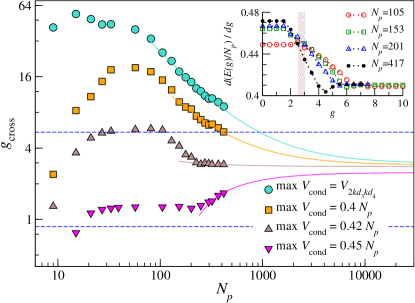
Figure 1: Value of $g_{\mathrm{cross}}(N,N_{p})$, solution of Eq. (14), as a function of $N_{p}$ with filling $N_{p}/N=3/10$ and screening length $R=10a$. Four different condensed subspaces (different $\max V_{\mathrm{cond}}$) are considered V2kd3kd4 . Numerical MC data (symbols) are extrapolated to $N_{p}\to\infty$ by fitting $A+B/N_{p}$ (solid lines) to the points with largest $N_{p}$. The horizontal dashed lines are the rigorous bounds of Eqs. (28) and (29). Inset: derivative of the GS energy per particle versus $g$ for different values of $N_{p}$. The shaded column indicates the value of $g_{c}=2.76\pm 0.24$ extrapolated as explained above.

Finally, we consider the limit $R\gg a$ in which screening becomes negligible. In this limit we are able to express the characteristic potential values, namely, $\min V/N_{p}$, $\max V/N_{p}$ and $\overline{V}/N_{p}$ in a closed analytical form SM We stress that these expressions are derived by first taking the $\operatorname{TD-lim}$ and then picking the leading term for $R\gg a$. By plugging these expressions together with $K_{0}/N_{p}\simeq-2\sin(\pi\varrho)/(\pi\varrho)$, obtained from Eq. (27) for $R\gg a$, into Eqs. (28) and (29), we find rs

$$\frac{\sin(\pi\varrho)/(2\pi\varrho^{2})}{\ln(R/a)-\varrho\ln(\varrho R/a)}\leq{r_{s}}_{c}\leq\frac{\sin(\pi\varrho)/(2\pi\varrho^{2})}{-\varrho\ln(\varrho)}.$$ (30)

Equation (30) allows us to estimate the dependence of ${r_{s}}_{c}$ on $\varrho$ in the range $a/R<\varrho\leq 1$, which, in virtue of the condition $R\gg a$, as a matter of fact coincides with the whole filling range.

In the limit $R/a\to\infty$, the lower bound of Eq. (30) vanishes whereas the upper bound remains finite. This is compatible with, but does not prove that ${r_{s}}_{c}\to 0$ in the limit of infinitely large screening length. However, from Weyl’s inequality $\min V(g+\min K/\min V)\leq\min H\leq\min V(g+\max K/\min V)$ and using the $R\gg a$ expressions of $K_{0}$ and $\min V$, we find

$$\lim_{R/a\to\infty}\operatorname{TD-lim}\frac{E(g)}{N_{p}}=\left\{\begin{array}[]{l}+\infty,\quad\quad\quad\leavevmode\nobreak\ g>0,\\ -2\frac{\sin(\pi\varrho)}{\pi\varrho},\quad g=0.\end{array}\right.$$ (33)

We conclude that, if the $\operatorname{TD-lim}$ is taken first, the Wigner crystallization is always realized as a first-order QPT of the type QPT but the critical parameter ${r_{s}}_{c}\to 0^{+}$ in the limit in which the potential becomes unscreened, $R/a\to\infty$.

Massimo Ostilli and Carlo Presilla

Appendix A Ground states of $K$ and $V$

For a ring of $N$ sites, the dimensionless hopping Hamiltonian is

$$K =-\sum_{i=1}^{N}\left(c^{\dagger}_{i}c_{i+1}+c^{\dagger}_{i+1}c_{i}\right).$$ (S1)

with $c_{i+N}=c_{i}$. The GS of $K$, $|K_{0}\rangle$, is the product state of the $N_{p}$ single-particle states with the lowest single-particle energies among $\epsilon_{n}=-2\cos(2\pi n/N)$, $n=0,\dots,N-1$. For $N_{p}$ odd the corresponding GS energy is

$$K_{0}=\min K=-2\sin(\pi N_{p}/N)/\sin(\pi/N).$$ (S2)

In the same ring, the dimensionless interaction potential reads

$$V=\sum_{i=1}^{N}\sum_{j=i+1}^{N}v_{i,j}c^{\dagger}_{i}c_{i}c^{\dagger}_{j}c_{j}=\sum_{i=1}^{N}\sum_{j=i+1}^{N}v_{i,j}n_{i}n_{j},$$ (S3)

with

$$v_{i,j}=\frac{1}{d_{i,j}}e^{-ad_{i,j}/R},$$ (S4)

where $d_{i,j}$ is the dimensionless distance between sites $i$ and $j$ in the ring

$$d_{i,j}=\min(j-i,N+i-j),\quad j>i.$$ (S5)

At filling $\varrho=p/q$, with $p$ and $q$ coprimes, there are $q$ degenerate classical WCs, i.e., $q$ configurations $(n_{1},n_{2},\dots,n_{N})$, with $n_{i}=0,1$ and $\sum_{i=1}^{N}n_{i}=N_{p}$, which realize the minimum value of the potential (S3). For $p=1$ these are configurations with equidistant fermions SM_Fratini2004 , while for $p>1$ we have a dimer structure SM_Hubbard1978 ; Slavin2005 . For instance, at filling $\varrho=3/10$, we have $\min V=V_{k(d_{3}d_{3}\mathrm{d}_{4})}$, which is the potential of the 10 nonequivalent configurations obtained by repeating $k=N_{p}/3=N/10$ times the sequence $d_{3}d_{3}\mathrm{d}_{4}$, where $d_{3}$ and $d_{4}$ are the so called 3-dimers $(\circ,\circ,\bullet)$ and 4-dimers $(\circ,\circ,\circ,\bullet)$, namely, lattice segments of 3 or 4 sites in which only the last one is occupied.

Appendix B Characteristic values of the screened Coulomb energy

The Wigner Crystallization cannot be clearly understood without an analysis of the distribution of the values of the classical potential. An example of this distribution is given in Fig. S1.

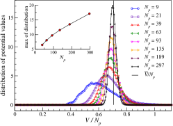
Figure S1: Distribution of $V/N_{p}$ from Eq. (S4) with screening length $R=10a$ and filling $\varrho=3/10$ obtained by random sampling up to $2^{26}$ configurations for different values of $N_{p}$. The vertical line at $\overline{V}/N_{p}$ indicates the Dirac delta distribution obtained in the $\operatorname{TD-lim}$. Inset: maximum value of the distribution as a function of $N_{p}$.

In the following, we evaluate the $\operatorname{TD-lim}$ necessary for the implementation of the equations of the Letter: $\min V/N_{p}$, $\max V/N_{p}$, the classical mean value ${\overline{V}}/{N_{p}}$, and the gap (see Eqs. (31)-(34) of the Letter). As we shall see, compact formulas can be provided in the important limit of large screening length, $R\gg a$. We shall also demonstrate why the distribution of $V/{N_{p}}$ tends to a Dirac delta distribution centered on the mean value.

B.1 Minimum of $V$

Let us evaluate the minima $\min V$, i.e., the value of $V$ evaluated in any of its $q$ GSs (we recall that the filling is $\varrho=p/q$ with $p$ and $q$ coprimes). The GS of $V$ takes the following expression

$$\min V=\sum_{j=1}^{N_{p}-1}v_{1,r(j)}+\sum_{j=r(1)}^{N_{p}-1}v_{r(1),r(j)}+\ldots,\leavevmode\nobreak\$$ (S6)

$$r(j)=1+[N/N_{p}]j+[(N/N_{p}-[N/N_{p}])j],$$ (S7)

where $[\cdot]$ stands for integer part and $r(j)$ represents the position of the $(j+1)$th particle SM_Slavin2005 . When $N/N_{p}$ is an integer (i.e., when $p=1$), we have $r(j)=1+N/N_{p}j$ and in the ring, where the distance is defined as in (S5), the above expression simplifies neatly in

$$\min V=\frac{N_{p}}{2}\sum_{j=1}^{N_{p}-1}v_{1,r(j)}.$$ (S8)

When instead $N/N_{p}$ is not an integer, the approximation $r(j)\simeq 1+N/N_{p}j$ will produce in general not integer values above and below the corresponding exact values of $r(j)$. For large values of $N$ and $N_{p}$ with $N_{p}/N$ fixed, these above and below approximations will tend to be somehow distributed around the exact values of $r(j)$. In such a limit we can hence still use Eq. (S8) as an approximation and, from the explicit expression of the $v_{i,j}$ we get (we suppose $N_{p}$ odd as in the Letter)

$$\min V\simeq N_{p}\sum_{j=1}^{(N_{p}-1)/2}\frac{e^{-d_{1,r(j)}a/R}}{d_{1,r(j)}},$$ (S9)

Note that in the above summation we have only $d_{i,j}=j-i$. In the following, we shall apply the same approximation to all the other terms, i.e., we will take $r(j)\simeq 1+jN/N_{p}$ (which amounts to $d_{1,r(j)}\simeq jN/N_{p}$) thoroughly. By using the variable $x=Naj/N_{p}R$, we get (now we take $N_{p}-1\simeq N_{p}$)

$$\min V\simeq N_{p}\frac{a}{R}\sum_{x=Na/N_{p}R}^{Na/2R}\frac{e^{-x}}{x},$$ (S10)

and

$$\operatorname{TD-lim}\frac{\min V}{N_{p}}\simeq\frac{a}{R}\sum_{x=a/\varrho R}^{\infty}\frac{e^{-x}}{x},$$ (S11)

which in turn gives

$$\lim_{R/a\gg 1}\operatorname{TD-lim}\frac{\min V}{N_{p}}\simeq\varrho\int_{a/\varrho R}^{\infty}dx\frac{e^{-x}}{x}.$$ (S12)

The above integral can be split as a part over the interval $[1,\infty]$ and a part over the interval $[a/\varrho R,1]$. The former is a finite dimensionless constant $I_{1}$, whereas the latter gives

$$\int_{a/\varrho R}^{1}dx\frac{e^{-x}}{x}=\ln(\varrho R/a)+I_{2}.$$ (S13)

where $I_{2}$ is another finite constant. In conclusion, we have

$$\lim_{R/a\gg 1}\operatorname{TD-lim}\frac{\min V}{N_{p}}\simeq\varrho\ln(\varrho R/a)+\mathop{O}(1).$$ (S14)

In general, in the limit $R/a\to\infty$ the term $\mathop{O}(1)$ is a small correction that depends on $\varrho$ and is exactly zero for densities such that $N/N_{p}$ is an integer. See Fig. S2.

B.2 Maximum of $V$

Let us calculate $\max V$, i.e., the maximum value of $V$ evaluated in any of the $N$ ways that exist to put the $N_{p}$ particles in $N_{p}$ consecutive sites. We have

$$\max V=v_{1,2}+ v_{1,3}+v_{1,4}+\ldots+v_{1,N_{p}}+\leavevmode\nobreak\$$

$$v_{2,3}+v_{2,4}+\ldots+v_{2,N_{p}}+\leavevmode\nobreak\$$

$$\quad\quad\quad\quad\leavevmode\nobreak\ +\ldots+\leavevmode\nobreak\$$

$$\quad\quad\quad\quad\quad\quad\leavevmode\nobreak\ \leavevmode\nobreak\ +v_{N_{p}-1,N_{p}},$$ (S15)

which, by using $v_{1,2}=v_{2,3}$, etc., gives

$$\max V=\sum_{n=1}^{N_{p}-1}(N_{p}-n)v_{1,n+1}.$$ (S16)

We can now proceed as in the previous case arriving at

$$\lim_{R/a\gg 1}\operatorname{TD-lim}\frac{\max V}{N_{p}}\simeq\left[\ln(R/a)+\mathop{O}(1)\right]-\lim_{R/a\gg 1}\operatorname{TD-lim}R\frac{e^{-a/R}}{N_{p}},$$ (S17)

or

$$\lim_{R/a\gg 1}\operatorname{TD-lim}\frac{\max V}{N_{p}}\simeq\ln(R/a)+\mathop{O}(1).$$ (S18)

Also in this case, in the limit $R/a\to\infty$ the term $\mathop{O}(1)$ is a small correction that depends on $\varrho$ and is exactly zero for densities such that $N/N_{p}$ is an integer. See Fig. S2.

B.3 Classical mean value and distribution of the normalized values $V/N_{p}$

The classical mean value of $V$ is defined as the average over all configurations. If we indicate by $\overline{\leavevmode\nobreak\ \cdot\leavevmode\nobreak\ }$ these averages, from Eq. (S3) we have

$$\overline{V}=\frac{\sum_{n}\langle n|V|n\rangle}{M}=\sum_{i=1}^{N}\sum_{j=i+1}^{N}v_{i,j}\overline{n_{i}n_{j}}.$$ (S19)

In Eq. (S19) one is tempted to neglect correlations and to replace $\overline{n_{i}n_{j}}$ with $\overline{n_{i}}\cdot\overline{n_{j}}=\varrho^{2}$. In this way we get

$$\frac{\overline{V}}{N_{p}}\simeq\frac{\varrho^{2}}{N_{p}}\sum_{i=1}^{N}\sum_{j=i+1}^{N}v_{i,j}.$$ (S20)

It turns out that this approximation becomes exact in the thermodynamic limit, however, the reason for that is quite not trivial. By analyzing the distribution of the classical $V/N_{p}$ values in the thermodynamic limit, we can simultaneously understand why Eq. (S20) becomes exact and why the distribution tends to a Dirac delta distribution centered at ${\overline{V}}/{N_{p}}$.

In general, $\min V$ is $q$-fold degenerate, whereas $\max V$ is $N$-fold degenerate, and as we consider more and more intermediate values of $V$, the degeneracy grows exponentially fast with the system size. This can be better understood in terms of entropy. Let us first consider the case $\varrho=1/q$ and let us split the $N$ sites into $N/q=N_{p}$ segments each made up of $q$ sites. Let us enumerate these segments from $j=1$ to $N_{p}$. In each segment, we can accommodate a number of particles $m_{j}$ between 0 and $q$ provided that the constrain $\sum_{j}m_{j}=N_{p}$ is satisfied. There are many possible ways to realize a given sequence of segments $\{m_{j}\}$ and the corresponding potential $V$ might be different for each one of such realizations. We are interested in counting the total number of configurations $\mathcal{N}(\{m_{j}\})$ associated to a given sequence of segments $\{m_{j}\}$, independently of the different values of $V$. Taking into account that the particles are indistinguishable and double occupancy of a site is forbidden, the number of configurations $\mathcal{N}(\{m_{j}\})$ associated to a given sequence of segments $\{m_{j}\}$ is

$$\mathcal{N}\Large(\{m_{j}\}\Large)=\delta\left(\sum_{j}m_{j}-N_{p}\right)\prod_{j}\binom{q}{m_{j}},$$ (S21)

For $N$ large, by a small variation of the sequence of segments we can have a large variation of $\mathcal{N}\large(\{m_{j}\}\large)$. In fact, not surprisingly, it is easy to check that, $\ln(\mathcal{N}\large(\{m_{j}\}\large))$, i.e., the canonical entropy, is exponentially peaked around its maximum which is attained by the uniform segment distribution, $\{m_{j}=1\}$. The important point here is that, at $\{m_{j}=1\}$, $V$ still depends on the particular realization of the uniform segment distribution and we are precisely interested in evaluating the mean value of these values of $V$ because in correspondence of the uniform segment distribution $\{m_{j}=1\}$ there are concentrated the most frequent values of $V$ (in fact, as the entropy shows, exponentially more frequent than the other values). For these values we have $V\in[\min V,\max V|_{\{m_{j}=1\}}]$, where $\min V$, as we already know, is obtained by putting, for example, all the particles in the rightmost position of the segments, and $\max V|_{\{m_{j}=1\}}$ is obtained by putting, for example, the particle of the $i$-th segment on the leftmost position of the segment when $i$ is odd, and on the rightmost position when $i$ is even. Notice that, for $\varrho<1/2$ (as thoroughly supposed in our work,) $\max V|_{\{m_{j}=1\}}$ is strictly lower than $\max V$ (it is easy in particular to evaluate it in the limit of large screening length, where we get $\max V|_{\{m_{j}=1\}}/N_{p}\simeq 2\varrho\ln(R/a)$, to be compared with $\max V/N_{p}\simeq\ln(R/a)$ from Eq. (S18)). Notice also that $\min V$, which is $q$-fold degenerate, and $\max V|_{\{m_{j}=1\}}$, which is $2q$-fold degenerate, are just two extremal values of the uniform segment distribution $\{m_{j}=1\}$ but they are not typical. The typical values of $V$ in the range $[\min V,\max V|_{\{m_{j}=1\}}]$ are more complicated and must have exponential degeneracies (or, more in general, nearly degeneracies).

We have so far shown that, in the $\operatorname{TD-lim}$, the distribution of $V/N_{p}$ tends to a Dirac delta distribution centered on its mean value which in turn must coincide with the mean value restricted to the uniform segment distribution, $\{m_{j}=1\}$. It is this latter fact that allows us to evaluate the mean of $V/N_{p}$ in a simple way: since in each segment we have exactly one particle, we are no more concerned with correlations so that the replacement $\overline{n_{i}n_{j}}$ with $\overline{n_{i}}\cdot\overline{n_{j}}=\varrho^{2}$, as in Eq. (S20), is actually exact in the $\operatorname{TD-lim}$. In other words, we can approximate the $N_{p}$ segments as uniformly occupied by a continuous distribution of charge of density $\varrho=1/q$. In particular, in the limit of large screening length Eq. (S20) provides

$$\lim_{R/a\gg 1}\operatorname{TD-lim}\frac{\overline{V}}{N_{p}}\simeq\varrho\ln(R/a)+\mathrm{O}(1).$$ (S22)

The above result has been derived for simplicity in the case $\varrho=1/q$, however, the same arguments can be equally repeated in the general case of $\varrho=p/q$ and the result is still Eqs. (S20) and (S22). See Fig. S2.

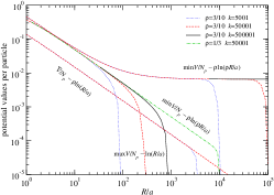
Figure S2: The exact minimum, maximum, and classical mean value of the potential $V$ per particle compared with the leading terms of Eqs. (S14), (S18), and (S22), respectively, as a function of the screening length $R/a$ for filling $\varrho=3/10$ and $\varrho=1/3$. The integer $k=1,2,\ldots$ determines the size of the system: we have $N_{p}=3k$ and $N=10k$ for filling $3/10$ and $N_{p}=k$ and $N=3k$ for filling $1/3$. Provided the system size is sufficiently large ($\operatorname{TD-lim}$ almost reached), when $1/\varrho$ is an integer, the difference between the exact values and the leading terms is always $O(1/(R/a))$ (here we show only the curve relative to $\min V$). When $1/\varrho$ is not an integer, the curve corresponding to $\min V$ tends to a small $\mathrm{O}(1)$ term. All curves show a drop for $R/a$ sufficiently large, meaning that the $\operatorname{TD-lim}$ cannot be considered reached at the used $k$ values for the shown values of $R/a$.

Appendix C Gap of $V$

The gap is defined as the difference between the first excited value of $V$ and its minimum. If $1/\varrho$ is integer (i.e., $p=1$), the former can be obtained by shifting one single particle in the GS of $V$ by one hop toward a first neighbor vacant position. By using the definitions (S5) and (S7), we have

$$\mathrm{gap}(V)=\sum_{j=1}^{N_{p}\leavevmode\nobreak\ -1}v_{2,r(j)}-\sum_{j=1}^{N_{p}-1}v_{1,r(j)}=\sum_{j=1}^{(N_{p}-1)/2}v_{2,r(j)}+\sum_{j=(N_{p}+1)/2}^{N_{p}-1}v_{2,r(j)}-2\sum_{j=1}^{(N_{p}-1)/2}v_{1,r(j)}.$$

On defining the variables $x=(jN/N_{p})a/R$, $x_{1}=(jN/N_{p}-1)a/R$, and $x_{2}=[N-(jN/N_{p}-1)]a/R$, we obtain

$$\mathrm{gap}(V)=\frac{a}{R}\left[\sum_{x_{1}=\min x_{1}}^{\max x_{1}}\frac{e^{-x_{1}}}{x_{1}}+\sum_{x_{2}=\min x_{2}}^{\max x_{2}}\frac{e^{-x_{2}}}{x_{2}}-2\sum_{x=\min x}^{\max x}\frac{e^{-x}}{x}\right],$$ (S23)

where

$$\min x=\frac{1}{\varrho}\frac{a}{R},\qquad\max x=\frac{N_{p}-1}{2\varrho}\frac{a}{R},$$

$$\min x_{1}=\frac{1-\varrho}{\varrho}\frac{a}{R},\qquad\max x_{1}=\frac{N_{p}-1-2\varrho}{2\varrho}\frac{a}{R},$$

$$\min x_{2}=\frac{2}{\varrho}\frac{a}{R},\qquad\max x_{2}=\frac{N_{p}+1}{2\varrho}\frac{a}{R}.$$

In the limit of large screening length we get

$$\lim_{R/a\gg 1}\operatorname{TD-lim}\mathrm{gap}(V)\simeq\varrho\int_{\frac{1-\varrho}{\varrho}\frac{a}{R}}^{\infty}dx_{1}\frac{e^{-x_{1}}}{x_{1}}+\varrho\int_{\frac{2}{\varrho}\frac{a}{R}}^{\infty}dx_{2}\frac{e^{-x_{2}}}{x_{2}}-2\varrho\int_{\frac{1}{\varrho}\frac{a}{R}}^{\infty}dx\frac{e^{-x}}{x},$$ (S24)

which gives

$$\lim_{R/a\gg 1}\operatorname{TD-lim}\mathrm{gap}(V)\simeq-\varrho\ln[2(1-\varrho)].$$ (S25)

Whereas for the cases $1/\varrho$ integer the above formula turns out to be almost exact (e.g., for $\varrho=1/3$, Eq. (S25) gives $\varrho\ln[2(1-\varrho)]=0.0958$, while the exact value of the gap is $0.0986$), when $1/\varrho$ is not an integer, it provides only a rough approximation since, for such cases, the first excited state of $V$ cannot be obtained by simply shifting one single particle in the GS of $V$. In particular, for $\varrho=3/10$ Eq. (S25) gives a value about 50 times larger than the actual value. In general, the first excited state of $V$ corresponds to a not trivial modification of its GS.

Appendix D Monte Carlo simulations

For finite size systems we can evaluate several properties of the GS by means of Monte Carlo simulations, other numerical methods being excluded due to the huge size of the Hilbert space. In the following, we discuss data obtained by an unbiased Monte Carlo code SM_MC1 based on an exact probabilistic representation of the quantum evolution operator SM_EPR1 . Note that we always simulate systems with an odd number of fermions in order to avoid any sign problem SM_Wiese . The code has been parallelized using openMP.

The relevant code parameters SM_MC1 that we used in our simulations are: $2^{14}$ stochastic trajectories (independent Poisson processes), $2^{12}$ reconfigurations and a time $3/N_{p}$ between consecutive reconfigurations (corresponding to about 10 jumps of the Poisson processes). For the largest simulated system with 417 particles in a lattice of 450 sites, this required a computation time of about 200 hours per single $g$ point for each subspace. Since the crossing between $E_{\mathrm{cond}}(g)$ and $E_{\mathrm{norm}}(g)$ can be obtained by simulating both these two GS energies in, at least, 2 $g$ points, we obtain a computation time for $g_{\mathrm{cross}}$ of about 800 hours. The absence of bias effects is checked by evaluating $E$ at $g=0$ and comparing the result with $K_{0}$, the GS energy of $K$, for which we have the explicit formula (S2). The total computation time at this size is, in conclusion, about 1000 hours.

In Fig. S3 we show the behavior of the energies per particle, $E_{\mathrm{cond}}/N_{p}$, $E_{\mathrm{norm}}/N_{p}$ and $E/N_{p}$, as a function of $g$ in the case $N_{p}=15$, $N=50$ and with the choice $\max V_{\mathrm{cond}}=0.4N_{p}$. It is evident that $E$ interpolates between $E_{\mathrm{norm}}$ at $g$ small and $E_{\mathrm{cond}}$ at $g$ large. The functions $E_{\mathrm{cond}}(g)$ and $E_{\mathrm{norm}}(g)$ intersect at $g_{\mathrm{cross}}\simeq 8.3$. Note that, whereas the values of $E_{\mathrm{cond}}$, $E_{\mathrm{norm}}$ and $g_{\mathrm{cross}}$ depend on the choice of the condensed subspace, univocal thermodynamic limits $\epsilon_{\mathrm{cond}}$, $\epsilon_{\mathrm{norm}}$ and $g_{c}$ are obtained for any allowed $\mathbb{F}_{\mathrm{cond}}$.

Figure 2 of the Letter is obtained by using also a suitable importance sampling which turns out to be effective at large values of $g$. Concerning the Inset of Fig. 2, where we evaluate $d(E(N,N_{p},g)/N_{p})/dg$, we have made use of the Savitsky-Golay filter SM_SG applied to the MC data in order to smooth the otherwise too noisy signal (by first applying the filter to the MC data and then evaluating the derivative, or by directly applying the filter to evaluate the derivative produce similar results; the Inset shows the latter).

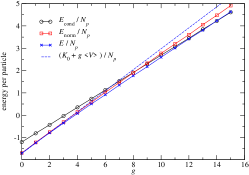
Figure S3: Energies per particle, $E_{\mathrm{cond}}/N_{p}$, $E_{\mathrm{norm}}/N_{p}$ and $E/N_{p}$, for the Hamiltonian $H=K+gV$ as a function of $g$. We have $N_{p}=15$, $N=50$ and screening length $R=10a$. As condensed subspace we use that defined by $V_{\mathrm{cond}}=0.4N_{p}$. The dashed line is the GS energy of $H$ obtained, at the first order of perturbation theory, considering $gV$ as a perturbation of $K$.

Appendix E Perturbation theory

We have not made use of any finite perturbation theory. The following represents only a complementary study that could be used for consistency.

For $g$ small, we can approximate the energy $E$ of the GS of $H$ by using the first order perturbation theory. We have $E=K_{0}+g\left\langle V\right\rangle$, where $\left\langle V\right\rangle=\langle K_{0}|V|K_{0}\rangle$ is

$$\left\langle V\right\rangle =\sum_{i=1}^{N}\sum_{j=i+1}^{N}\frac{e^{-ad_{i,j}/R}}{d_{i,j}}\left(\frac{N_{p}}{N}\right)^{2}$$

$$\qquad\times\left[1-\left(\frac{\sin(\pi N_{p}(j-i)/N)}{N_{p}\sin(\pi(j-i)/N)}\right)^{2}\right].$$ (S26)

In terms of limiting rescaled energies we thus conclude that for $g$ small (see Fig. S3)

$$\epsilon_{\mathrm{norm}}\simeq\operatorname{TD-lim}\frac{K_{0}}{N_{p}}+g\operatorname{TD-lim}\frac{\left\langle V\right\rangle}{N_{p}}.$$

Remark. The GS of $K+gV$ tends to $|K_{0}\rangle$, or to one of the classical WCs, in the limits $g\to 0$ and $g\to\infty$, respectively. Now, whereas for $g$ sufficiently small is safe to assume that the actual GS is a slight deformation of $|K_{0}\rangle$, i.e., a product state of single particle Bloch waves, the investigation of the actual GS for $g$ sufficiently large is quite more complex. In fact, depending on $p$, different ansatzs have been proposed in the past: a Bloch superposition of kink-antikink configurations for $p=1$ SM_Fratini2004 , and of excited dimers for $p>1$ SM_Slavin2005 . However, whereas these ansatzs provide physical appealing insights, they remain heuristic as essentially focus on single mode excitations. There is no reason to exclude a priori that an extensive number of kink-antikink walls ($p=1$), or other nondimer configurations ($p>1$) concur to the actual GS for $g$ finite. In fact, in both cases, the potential values associated to the configurations contributing to these Bloch states differ from the energy of the WCs (i.e., the minima of $V$) by terms $O(1)$, while our condition (ii) on $\mathbb{F}_{\mathrm{cond}}$ requires a larger space, being $\max V_{\mathrm{cond}}=\min V+O(N_{p})$, and only under such a condition a QPT can be reached.

Appendix F Monotonicity and convexity of the GS energies

Consider the Taylor expansion and the infinite perturbation series of the GS energy $E(g)$ both around an arbitrary $g$ and compare term by term the first- and second-order terms of the two expansions. By using the fact that the first-order term of the perturbation series is $\langle E(g)|V|E(g)\rangle/\langle E(g)|E(g)\rangle\geq 0$, we get $\partial E(g)/\partial g\geq 0$ (this result can be equally reached by using the Hellman-Feynman theorem). Next, by using the fact that the second-order term of the perturbation series for the GS energy is always negative or null, we also get $\partial^{2}E(g)/\partial g^{2}\leq 0$. The same argument applies to $E_{\mathrm{cond}}$ and $E_{\mathrm{norm}}$. In conclusion, with respect to $g$, all the GS energies are functions that are monotone increasing and convex upward.

Appendix G Proof that Eq. (9) implies $\min K_{\mathrm{norm}}/K_{0}=1$ in the $\operatorname{TD-lim}$

The starting point is the exact probabilistic representation of the quantum evolution introduced in SM_EPR1 . According to this exact representation, at an imaginary time $t$, we have

$$\langle\bm{n}|e^{-Ht}|\bm{n}_{0}\rangle=\mbox{$\mathsf{E}$}\left(\mathcal{M}^{[0,t)}_{\bm{n}_{0}}\delta_{\bm{n}_{N_{t}},\bm{n}}\right),$$ (S27)

where $\mbox{$\mathsf{E}$}(\cdot)$ is the probabilistic expectation over the continuous time Markov chain of configurations $\bm{n}_{0},\bm{n}_{s_{1}},\dots,\bm{n}_{s_{N_{t}}}$ (or trajectory) defined by the transition matrix

$$P_{\bm{n},\bm{n}^{\prime}}=\frac{|\langle\bm{n}|K|\bm{n}^{\prime}\rangle|}{A(\bm{n})},\qquad A(\bm{n})=\sum_{\bm{n}^{\prime}}|\langle\bm{n}|K|\bm{n}^{\prime}\rangle|,$$ (S28)

and the sequence of jumping times $s_{1},s_{2},\dots,s_{N_{t}}$ obtained from the Poissonian conditional probability density

$$P(s_{k}|s_{k-1})=e^{-\Gamma A(\bm{n}_{s_{k-1}})(s_{k}-s_{k-1})}\Gamma A(\bm{n}_{s_{k-1}}).$$ (S29)

Concretely, starting form the configuration $\bm{n}_{0}$ at time $s_{0}=0$, we draw a configuration $\bm{n}_{s_{1}}$ with probability $P_{\bm{n}_{0},\bm{n}_{s_{1}}}$ at time $s_{1}$ drawn with probability density $P(s_{1}|s_{0})$, then we draw a configuration $\bm{n}_{s_{2}}$ with probability $P_{\bm{n}_{s_{1}},\bm{n}_{s_{2}}}$ at time $s_{2}$ drawn with probability density $P(s_{2}|s_{1})$, and so on until we reach the configuration $\bm{n}_{N_{t}}$ at time $s_{N_{t}}$ such that $s_{N_{t}+1}>t$. Note that the Poisson processes associated to each jump are defined left continuous SM_EPR1 , as a consequence, the configuration $\bm{n}_{N_{t}}$ is the one realized by the Markov chain just before the final time $t$. The stochastic functional $\mathcal{M}^{[0,t)}_{\bm{n}_{0}}$ is then defined as

$$\mathcal{M}^{[0,t)}_{\bm{n}_{0}} =e^{\sum_{k=0}^{N_{t}-1}[\Gamma A(\bm{n}_{s_{k}})-V(\bm{n}_{s_{k}})](s_{k+1}-s_{k})}\cdots e^{[\Gamma A(\bm{n}_{s_{N_{t}}})-V(\bm{n}_{s_{N_{t}}})](t-s_{N_{t}})},$$ (S30)

where $A(\bm{n})$ is called the number of links, or degree of $\bm{n}$, and represents the number of non-null off-diagonal matrix elements $\langle\bm{n}|H|\bm{n}^{\prime}\rangle$.

The exact probabilistic representation (S27) is at the base of the unbiased Monte Carlo simulations used to sample the GS properties (by sending the imaginary time $t$ to sufficiently large values), as explained before (see Figs. S2 and S3). Eq. (S27), however, lends itself also to quite interesting analytical treatments allowing for a direct connection between GS properties and the (virtual) trajectories of the Markov chain SM_ANAL ; ANAL1 . Here we consider the case with no interaction $V\equiv 0$ and $N_{p}$ odd, i.e., a lattice chain of spinless fermions with no sign problem (equivalent to a system of hard-core bosons). As done in SM_ANAL , in this particular case we can easily decompose the expectation of the stochastic functional $\mathcal{M}^{[0,t)}_{\bm{n}_{0}}$ as a sum over trajectories that, starting from a given initial configuration ${\bm{n}_{0}}$, perform $N_{t}=k$ jumps within the time $t$. By integrating out the ordered jumping times $s_{1},s_{2},\dots,s_{k}$ distributed according to the probability density (S29), and by using $\int_{0}^{t}\Gamma ds_{1}\int_{s_{1}}^{t}\Gamma ds_{2}\ldots\int_{s_{k-1}}^{t}\Gamma ds_{k}=(\Gamma t)^{k}/(k!)$, we arrive at

$$\sum_{\bm{n}}\langle\bm{n}|e^{-Ht}|\bm{n}_{0}\rangle=\mbox{$\mathsf{E}$}\left(\mathcal{M}^{[0,t)}_{\bm{n}_{0}}\right)=\sum_{k}^{\infty}\frac{(\Gamma t)^{k}}{k!}\mathcal{N}(\bm{n}_{0};k),$$ (S31)

where $\mathcal{N}(\bm{n}_{0};k)$ counts the total number of trajectories having $k$ jumps (each starting from $\bm{n}_{0}$). Similarly, for the Hamiltonians $H_{\mathrm{cond}}$ and $H_{\mathrm{norm}}$ defined as the Hamiltonian $H$ restricted to the subspaces $\mathbb{F}_{\mathrm{cond}}$ and $\mathbb{F}_{\mathrm{norm}}$, respectively, we have

$$\sum_{\bm{n}\in\mathbb{F}_{\mathrm{cond}}}\langle\bm{n}|e^{-H_{\mathrm{cond}}t}|\bm{n}_{\mathrm{cond}}\rangle=\sum_{k}^{\infty}\frac{(\Gamma t)^{k}}{k!}\mathcal{N}_{\mathrm{cond}}(\bm{n}_{\mathrm{cond}};k),$$ (S32)

$$\sum_{\bm{n}\in\mathbb{F}_{\mathrm{norm}}}\langle\bm{n}|e^{-H_{\mathrm{norm}}t}|\bm{n}_{\mathrm{norm}}\rangle=\sum_{k}^{\infty}\frac{(\Gamma t)^{k}}{k!}\mathcal{N}_{\mathrm{norm}}(\bm{n}_{\mathrm{norm}};k),$$ (S33)

where $\bm{n}_{\mathrm{cond}}$ and $\bm{n}_{\mathrm{norm}}$ are two arbitrary initial configurations of $\mathbb{F}_{\mathrm{cond}}$ and $\mathbb{F}_{\mathrm{norm}}$, respectively. On expanding the lhs of these equations to leading order in $t$ we get

$$\sum_{\bm{n}}\langle\bm{n}|\bm{n}_{0}\rangle e^{-Et}=\sum_{k}^{\infty}\frac{(\Gamma t)^{k}}{k!}\mathcal{N}(\bm{n}_{0};k),$$ (S34)

$$\sum_{\bm{n}\in\mathbb{F}_{\mathrm{cond}}}\langle\bm{n}|\bm{n}_{\mathrm{cond}}\rangle e^{-E_{\mathrm{cond}}t}=\sum_{k}^{\infty}\frac{(\Gamma t)^{k}}{k!}\mathcal{N}_{\mathrm{cond}}(\bm{n}_{\mathrm{cond}};k),$$ (S35)

$$\sum_{\bm{n}\in\mathbb{F}_{\mathrm{norm}}}\langle\bm{n}|\bm{n}_{\mathrm{norm}}\rangle e^{-E_{\mathrm{norm}}t}=\sum_{k}^{\infty}\frac{(\Gamma t)^{k}}{k!}\mathcal{N}_{\mathrm{norm}}(\bm{n}_{\mathrm{norm}};k).$$ (S36)

On the other hand, taking into account that $\mathcal{N}_{\mathrm{cond}}(\bm{n}_{\mathrm{cond}};k)$ and $\mathcal{N}_{\mathrm{norm}}(\bm{n}_{\mathrm{norm}};k)$ are fast growing functions of the space dimensions $M_{\mathrm{cond}}$ and $M-M_{\mathrm{cond}}$, respectively, if condition (9a) is satisfied, $\operatorname{TD-lim}{M_{\mathrm{cond}}/M}=0$, independently from the choice of the initial configurations, we clearly see that, for system size sufficiently large, and for any $k$ larger than some finite threshold

$$\mathcal{N}_{\mathrm{norm}}(\bm{n}_{\mathrm{norm}};k)>\mathcal{N}_{\mathrm{cond}}(\bm{n}_{\mathrm{cond}};k).$$ (S37)

Comparing Eqs. (S35) and (S36) we therefore conclude that, for system size sufficiently large,

$$E_{\mathrm{norm}}<E_{\mathrm{cond}},$$ (S38)

which, plugged into Eq. (9b), proves that $\min K_{\mathrm{norm}}/K_{0}=1$ in the $\operatorname{TD-lim}$.

References

• (1) E. Wigner, On the interaction of electrons in metals, Phys. Rev. 46, 1002 (1934).
• (2) J. Hubbard, Generalized Wigner lattices in one dimension and some applications to tetracyanoquinodimethane(TCNQ) salts, Phys. Rev. B 17, 494 (1978).
• (3) S. E. Burkov and Y. G. Sinai, Phase diagrams of one-dimensional lattice models with long-range antiferromagnetic interaction, Russ. Math. Surv. 38, 235 (1983).
• (4) P. Bak and R. Bruinsma, One-Dimensional Ising Model and the Complete Devil’s Staircase, Phys. Rev. Lett. 49, 249 (1982).
• (5) S. Fratini, B. Valenzuela, and D. Baeriswyl, Incipient quantum melting of the one-dimensional Wigner lattice, Synth. Met. 141, 193 (2004).
• (6) V. Slavin, Low-energy spectrum of one-dimensional generalized Wigner lattice, Phys. Status Solidi B 242, 2033 (2005).
• (7) B. Tanatar and D. M. Ceperley, Ground state of the two-dimensional electron gas, Phys. Rev. B 39, 5005 (1989).
• (8) F. Rapisarda and G. Senatore, Diffusion Monte Carlo study of electrons in two-dimensional layers, Aust. J. Phys. 49, 161 (1996).
• (9) C. Attaccalite, S. Moroni, P. Gori-Giorgi, and G. B. Bachelet, Correlation Energy and Spin Polarization in the 2D Electron Gas, Phys. Rev. Lett. 88, 256601 (2002).
• (10) N. D. Drummond and R. J. Needs, Phase Diagram of the Low-Density Two-Dimensional Homogeneous Electron Gas, Phys. Rev. Lett. 102, 126402 (2009).
• (11) M. Zarenia, D. Neilson, B. Partoens, and F. M. Peeters, Wigner crystallization in transition metal dichalcogenides: A new approach to correlation energy, Phys. Rev. B 95, 115438 (2017).
• (12) Y. Noda and M. Imada, Quantum Phase Transitions to Charge-Ordered and Wigner-Crystal States under the Interplay of Lattice Commensurability and Long-Range Coulomb Interactions, Phys. Rev. Lett. 89, 176803 (2002).
• (13) M. Siegmund, M. Hofmann, and O. Pankratov, Density functional study of collective electron localization: Detection by persistent current, J. Phys. Condens. Matter 21 155602 (2009).
• (14) B. Valenzuela, S. Fratini, and D. Baeriswyl, Charge and spin order in one-dimensional electron systems with long-range Coulomb interactions, Phys. Rev. B 68, 045112 (2003).
• (15) I. Shapir, A. Hamo, S. Pecker, C. P. Moca, Ö Legeza, G. Zarand and S. Ilani,Imaging the electronic Wigner crystal in one-dimension, Science, 364, 870 (2019).
• (16) D. H. E. Dubin, Minimum energy state of the one-dimensional Coulomb chain, Phys. Rev. E 55, 4017 (1997).
• (17) H. J. Brascamp, E. H. Lieb, Some inequalities for Gaussian measures and the long-range order of the one-dimensional plasma, edited by M. Loss and M. B. Ruskai, in Inequalities (Springer, Berlin, Heidelberg, 2002).
• (18) M. Ostilli and C. Presilla, First-order quantum phase transitions as condensations in the space of states, J. Phys. A 54, 055005 (2021).
• (19) M. Ostilli and C. Presilla, Exact Monte Carlo time dynamics in many-body lattice quantum systems, J. Phys. A 38, 405 (2005).
• (20) The relation between our parameter $g$ and the parameter $r_{s}$ usually appearing in the literature is as follows. In a one-dimensional lattice of spacing $a$ with $N$ sites and $N_{p}$ electrons, the radius of the volume available to each electron is $r=(aN/N_{p})/2$. Therefore $r_{s}\equiv r/a_{B}=g/4\varrho$.
• (21) See Supplemental Material at ¡url¿ for details, which includes Refs. Wiese ; SG ; ANAL ; ANAL1 .
• (22) M. Troyer and U.-J. Wiese, Computational Complexity and Fundamental Limitations to Fermionic Quantum Monte Carlo Simulations, Phys. Rev. Lett. 94, 170201 (2005).
• (23) A. Savitzky and M. J. E. Golay, Smoothing and differentiation of data by simplified least squares procedures, Anal. Chem., 36, 1627 (1964).
• (24) M. Ostilli and C. Presilla, An analytical probabilistic approach to the ground state of lattice quantum systems: Exact results in terms of a cumulant expansion, J. Stat. Mech., (2005) P04007.
• (25) M. Ostilli and C. Presilla, The exact ground state for a class of matrix Hamiltonian models: Quantum phase transition and universality in the thermodynamic limit, J. Stat. Mech., (2006) P11012.
• (26) J. N. Franklin Matrix Theory, (Dover Publications, New York, 1993).
• (27) At this filling $\min V=V_{k(d_{3}d_{3}\mathrm{d}_{4})}$, which is the potential associated to the so-called dimer configuration $d_{3}d_{3}\mathrm{d}_{4}$ repeated $k=N_{p}/3=N/10$ times, see Refs. Hubbard1978 ; Slavin2005 and comments in Ref. SM .
• (28) M. Beccaria, C. Presilla, G. F. De Angelis, and G. Jona Lasinio, An exact representation of the fermion dynamics in terms of Poisson processes and its connection with Monte Carlo algorithms, Europhys. Lett. 48, 243 (1999).
• (29) K. Binder, Finite Size Scaling Analysis of Ising Model Block Distribution Functions, Z. Phys. B 43, 119-140 (1981).
• (30) The potential $\max V_{\mathrm{cond}}=V_{2kd_{3}k\mathrm{d}_{4}}$ is the potential of the most excited configuration with $2k$ dimers $d_{3}$ and $k$ dimers $\mathrm{d}_{4}$, where $k=N_{p}/3=N/10$. The value $V_{2kd_{3}k\mathrm{d}_{4}}/N_{p}$ depends on $N_{p}$ but in $\operatorname{TD-lim}$ $V_{2kd_{3}k\mathrm{d}_{4}}/N_{p}\to 0.3925$.
Supplemental Material for

References

• (1) S. Fratini, B. Valenzuela, and D. Baeriswyl, “Incipient quantum melting of the one-dimensional Wigner lattice”, Synthetic Metals 141, 193 (2004).
• (2) J. Hubbard, “Generalized Wigner lattices in one dimension and some applications to tetracyanoquinodimethane(TCNQ) salts”, Phys. Rev. B 17, 494 (1978).
• (3) V. Slavin, “Low-energy spectrum of one-dimensional generalized Wigner lattice”, Phys. Stat. Sol. (b) 242, 2033 (2005).
• (4) M. Ostilli and C. Presilla, “Exact Monte Carlo time dynamics in many-body lattice quantum systems”, J. Phys. A 38, 405 (2005).
• (5) M. Beccaria, C. Presilla, G. F. De Angelis, G. Jona Lasinio, “An exact representation of the fermion dynamics in terms of Poisson processes and its connection with Monte Carlo algorithms ”, Europhys. Lett. 48, 243 (1999).
• (6) M. Troyer, U.-J. Wiese, “Computational Complexity and Fundamental Limitations to Fermionic Quantum Monte Carlo Simulations”, Phys. Rev. Lett. 94, 170201 (2005).
• (7) A. Savitzky, M. J. E. Golay, “Smoothing and Differentiation of Data by Simplified Least Squares Procedures”, Analytical Chemistry, 36, 1627 (1964).
• (8) M. Ostilli and C. Presilla, “An analytical probabilistic approach to the ground state of lattice quantum systems: exact results in terms of a cumulant expansion”, J. Stat. Mech., P04007 (2005).
• (9) M. Ostilli and C. Presilla, “The Exact ground state for a class of matrix Hamiltonian models: quantum phase transition and universality in the thermodynamic limit”, J. Stat. Mech., P11012 (2006).