Forman-Ricci curvature and Persistent homology of unweighted complex networks

Abstract

We present the application of topological data analysis (TDA) to study unweighted complex networks via their persistent homology. By endowing appropriate weights that capture the inherent topological characteristics of such a network, we convert an unweighted network into a weighted one. Standard TDA tools are then used to compute their persistent homology. To this end, we use two main quantifiers: a local measure based on Forman’s discretized version of Ricci curvature, and a global measure based on edge betweenness centrality. We have employed these methods to study various model and real-world networks. Our results show that persistent homology can be used to distinguish between model and real networks with different topological properties.

1 Introduction

Recent advances in topological data analysis (TDA) Zomorodian and Carlsson (2005); Edelsbrunner and Harer (2008); Carlsson (2009) have made it a powerful tool in data science. TDA has lead to important applications in different areas of science. For example, in astrophysics, TDA has be used for analysis of the Cosmic Microwave Background (CMB) radiation data Pranav et al. (2016); in imaging, TDA has been used for feature detection in 3D gray-scale images Günther et al. (2011); in biology, TDA has been used for detection of breast cancer type with high survival rates Nicolau et al. (2011) and understanding cell fate from single-cell RNA sequencing data Rizvi et al. (2017). The main tool in TDA is that of persistent homology Zomorodian and Carlsson (2005); Edelsbrunner and Harer (2008); Carlsson (2009), which has the power to detect the topology of the underlying data. The field of algebraic topology Munkres (2018) provides the basic mathematical tool required for TDA, namely that of homology. The conceptual roots of persistent homology, however, are in differential topology, in particular Morse theory Edelsbrunner and Harer (2008).

Network science Watts and Strogatz (1998); Barabási and Albert (1999); Albert and Barabási (2002); Newman (2010); Barabási (2016), on the other hand, investigates the topological and dynamical properties of various complex networks, that encode interactions between various agents in the natural as well as artificial setting. The ability to understand and predict the nature of these interactions is a key challenge. Historically, graph theory Bollobas (1998); Newman (2010); Barabási (2016) has provided the main tools and techniques for studying such networks, via their graph representation. Although graph theory has provided significant insights into such problems, recent studies have shown that such techniques do not adequately capture higher-order interactions and correlations arising in networks De Silva and Ghrist (2007); Horak et al. (2009); Petri et al. (2013, 2014); Bianconi (2015); Wu et al. (2015); Sizemore et al. (2016); Courtney and Bianconi (2017); Ritchie et al. (2017); Courtney and Bianconi (2018); Kartun-Giles and Bianconi (2019); Iacopini et al. (2019); Kannan et al. (2019). These higher-order phenomena can be encoded in hypergraph Klamt et al. (2009); Zlatić et al. (2009) and simplicial complex De Silva and Ghrist (2007); Horak et al. (2009); Lee et al. (2012); Petri et al. (2013, 2014); Sizemore et al. (2016); Iacopini et al. (2019) representations of networks. The tools of TDA are applicable to any simplicial complex and can be used to determine the important topological characteristics of networks. In this work, we employ TDA to study the persistent homology of unweighted and undirected simple graphs arising from model and real-world networks.

Previous research in this direction have investigated the persistent homology of weighted and undirected networks Petri et al. (2013, 2014). The filtration scheme required to compute persistent homology in weighted networks was then provided by the edge weights Petri et al. (2013, 2014). However, this technique is not immediately applicable to unweighted graphs due to the absence of edge weights. At present, due to insufficient information, the interaction networks underlying many real-world complex systems are available only as unweighted and undirected graphs. Examples of such unweighted and undirected real networks include the Yeast protein interaction network Jeong et al. (2001), the US Power Grid network Leskovec et al. (2007) and the Euro road network Šubelj and Bajec (2011). In order to reveal the higher-order topological features of such real-world networks, it is important to develop methods to study persistent homology in unweighted and undirected networks. A simple way to devise such a method would be to transform the given unweighted graph into an edge-weighted graph by assigning certain weights to all edges, and then, using the induced filtration to compute persistent homology. However, a priori it is not evident which edge weighting scheme would capture the topological characteristics of different types of unweighted networks.

Previously, Horak et al. Horak et al. (2009) used a dimension-based weighting scheme for unweighted networks where the weights are simply the dimension of the simplices. In particular, Horak et al. assign all edges with the weight $+1$ to study persistent homology in unweighted networks. However, we have recently shown that the dimension-based filtration scheme of Horak et al., though computationally fast, may not be able to conclusively distinguish between various model networks Kannan et al. (2019). In recent work Kannan et al. (2019), we gave another weighting method based on a discrete Morse function as introduced by Robin Forman Forman (1998, 2002), which assigns weights to each simplex in the clique complex corresponding to the unweighted graph according to a global acyclicity constraint. This method Kannan et al. (2019) simplifies the topological structure of the underlying simplicial complex, that leads to a computationally efficient way to compute homology and persistent homology. Moreover, we also showed that the persistent homology computed using this method was able to distinguish various unweighted model networks having different topological characteristics, the difference being quantified by the averaged bottleneck distance between the corresponding persistence diagrams Kannan et al. (2019). A natural question then is whether other choices of weights can also be used to distinguish such unweighted networks via persistent homology.

In the present contribution, we shall use both local and global network quantifiers for obtaining edge weighting schemes to compute persistent homology, namely that of discrete Ricci curvature Forman (2003); Sreejith et al. (2016, 2017); Samal et al. (2018), also introduced by R. Forman Forman (2003), which plays the role of local curvature in a discrete setting, and edge betweenness centrality Freeman (1977); Girvan and Newman (2002); Newman (2010) which is an edge-based measure analogous to the classical betweenness centrality for vertices of a graph. We shall show that the simpler methods introduced here to study persistent homology based on Forman-Ricci curvature or edge betweenness centrality are also able to distinguish unweighted model networks like our recent method Kannan et al. (2019) based on discrete Morse functions. However, note that the advantages in topological simplification and computational efficiency that result from using a discrete Morse function are lost with the simpler method presented here. Nevertheless, if the sole goal is to compute persistent homology in unweighted networks, the weighting schemes presented here are likely to be much simpler to use in practice. In this context, we have also applied our methods to study the persistent homology of some real-world networks. Note that our recent method based on discrete Morse functions Kannan et al. (2019) and the simpler methods presented here based on Forman-Ricci curvature or edge betweenness centrality are much better at distinguishing between different types of model networks in comparison to dimension-based method of Horak et al. Horak et al. (2009).

The remainder of the paper is organized as follows. In the Theory section, we present an overview of the concepts needed to study persistent homology in unweighted networks based on Forman-Ricci curvature and edge betweenness centrality. In the Datasets section, we describe the model and real networks analyzed here. In the Results section, we describe our new methods to study persistent homology in unweighted networks, and its application to both model and real-world networks. In the last section, we conclude with a brief summary and future outlook.

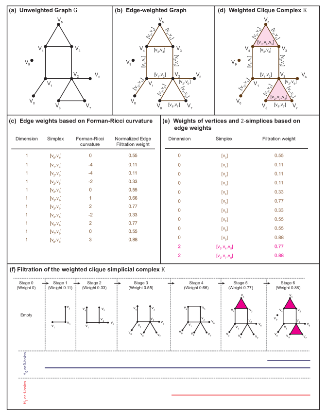
Figure 1: Schematic figure illustrating our method to study persistent homology in an unweighted and undirected network using Forman-Ricci curvature. (a) An example of an unweighted graph $G$. (b) Transformation of the unweighted graph into an edge-weighted graph using Forman-Ricci curvature. (c) Assignment of normalized filtration weights to edges in the weighted graph shown in (b) based on Forman-Ricci curvature. (d) Weighted clique simplicial complex $K$ corresponding to the unweighted graph $G$. (e) Assignment of normalized filtration weights to vertices ($0$-simplices) and $2$-simplices in the weighted clique complex shown in (d) based on edge weights. (f) Filtration of the weighted clique complex $K$ based on the ascending sequence of weights assigned to simplices. Barcodes depict that there is a $0$-hole (or connected component) that persists across the 6 stages of the filtration while another $0$-hole is born at the last stage on addition of the isolated vertex $v_{9}$. Moreover, a $1$-hole is born at stage 4 on addition of the edge $[v_{3},v_{4}]$.

2 Theory

2.1 Clique complex of a graph

Let $G(V,E)$ be a finite simple graph with $V$ being the set of vertices and $E$ being the set of edges. Each edge in the graph $G$ is an unordered pair of distinct vertices. We remark that a simple graph does not contain self-loops or multi-edges Bollobas (1998). An induced subgraph $K$ of $G$ that is complete is called a clique. We can view $G$ as a finite clique simplicial complex $K$ where a $p$-dimensional simplex (or $p$-simplex) is determined by a set of $p+1$ vertices that form a clique Zomorodian and Carlsson (2005); Edelsbrunner and Harer (2008). Specifically, a $p$-simplex is a polytope which is the convex hull of its $p+1$ vertices. Note that a simplex can be thought of as a generalization of points, lines, triangles, tetrahedron, and so on in higher dimensions. In the clique complex $K$, $0$-simplices correspond to vertices in $G$, $1$-simplices to edges in $G$, $2$-simplices to triangles in $G$, and so on. Given a $p$-simplex $\alpha$ in $K$, a face $\gamma$ of $\alpha$ is determined by a subset of the vertex set of $\alpha$ of cardinality less than or equal to $p+1$. Dually, a co-face $\beta$ of $\alpha$ is a simplex that contains $\alpha$ as a face. The dimension of a clique simplicial complex $K$ is the maximum dimension of its constituent simplices. An orientation of a $p$-simplex is given by an ordering of its constituent vertices Munkres (2018). Moreover, two orientations of a simplex are equivalent if they differ by an even permutation of its vertices.

2.2 Persistent homology of a simplicial complex

A simplicial complex is a collection $K$ of simplices which satisfies following two properties Munkres (2018). Firstly, any face $\gamma$ of a simplex $\alpha$ in $K$ is also included in $K$. Secondly, if two simplices $\alpha$ and $\beta$ in $K$ have a non-empty intersection $\gamma$, then $\gamma$ is a common face of $\alpha$ and $\beta$. A subcomplex $K^{\prime}$ of a simplicial complex $K$ is a collection of simplices in $K$ such that $K^{\prime}$ is also a simplicial complex. A filtration on a simplicial complex $K$ is given by a nested sequence of subcomplexes $K_{i}$, $i=0,1,\ldots,n$, such that:

$$\emptyset=K_{0}\subseteq K_{1}\subseteq\ldots\subseteq K_{n}=K.$$

For a simplicial complex $K$ with a given filtration, one can define its persistent homology groups as follows. First we fix a base field $\mathbb{F}$ Munkres (2018). The set of all oriented $p$-simplices in $K$ generate a free group $C_{p}$ over $\mathbb{F}$, called $p^{\text{th}}$-chain group Munkres (2018). An element in $C_{p}$ is called a $p$-chain, and is given by a finite formal sum:

$$C_{p}=\sum_{i=1}^{N}c_{i}\alpha_{i}$$

where the coefficients $c_{i}$ are in $\mathbb{F}$, and $\alpha_{i}$ are oriented $p$-simplices in $K$ Munkres (2018). Component-wise addition endows $C_{p}$ with the structure of a group, whose identity element is given by the unique $p$-chain with all coefficients $c_{i}$ equal to zero. If a $p$-simplex $\alpha$ is given an opposite orientation, then it is represented as $-\alpha$ in $C_{p}$, and gives the inverse of $\alpha$ in $C_{p}$. To define the persistent homology groups, we use the so-called boundary operator $\partial_{p}$, which is a map $\partial_{p}:C_{p}\rightarrow C_{p-1}$.

For an oriented $p$-simplex $\alpha=[x_{0},x_{1},\ldots,x_{p}]$ (i.e., the ordered vertex set $\{x_{0},x_{1},\ldots,x_{p}\}$ of $\alpha$), we define the boundary operator $\partial_{p}$ as:

$$\partial_{p}(\alpha)=\sum_{i=0}^{p}(-1)^{i}[x_{0},\ldots,\hat{x}_{i},\ldots,x_{p}]$$

where $[x_{0},\ldots,\hat{x}_{i},\ldots,x_{p}]$ denotes the $(p-1)$-face of $\alpha$ obtained by removing the vertex $x_{i}$ Munkres (2018). Since the right hand side of the above equation is a linear combination of $(p-1)$-simplices, it belongs to $C_{p-1}$. One can then extend the definition of $\partial_{p}$ to all elements of $C_{p}$ by linearity. The boundary operators satisfy the fundamental property:

$$\partial_{p}\circ\partial_{p+1}=0.$$

The kernel of the boundary operator is called the group of $p$-cycles and denoted by $Z_{p}$ Munkres (2018). It is given by the set of elements in $C_{p}$ that is mapped to $0$ in $C_{p-1}$ by the boundary operator $\partial_{p}$:

$$Z_{p}=\operatorname{Ker}(\partial_{p})=\{c\in C_{p}|\partial_{p}(c)=0\}.$$

A $p$-boundary is a $p$-cycle which lies in the image of the boundary operator $\partial_{p+1}$. The set of $p$-boundaries is denoted by $B_{p}$ and is a subgroup of $Z_{p}$ Munkres (2018).

$$B_{p}=\operatorname{Image}(\partial_{p+1})=\{c\in C_{p}|\exists b\in C_{p+1},\partial_{p+1}(b)=c\}.$$

Thus, the $p$-homology group is defined as Munkres (2018):

$$H_{p}(K)=\frac{Z_{p}(K)}{B_{p}(K)}.$$

Note that $H_{p}$ is a vector space over the field $\mathbb{F}$. The $p$-Betti number $\beta_{p}$ is given by the dimension of the homology group $H_{p}$. Informally, $\beta_{p}$ represents the number of holes in the $p$-homology group.

Now, every subcomplex $K_{i}$ in the filtration of the simplicial complex $K$ has an index $i$ associated with it. Also, for each $K_{i}$ there exists its corresponding $p$-chain, $p$-boundary operators, and thus, $p$-boundaries and $p$-cycles. We shall denote the $p$-cycles of $K_{i}$ as $Z^{i}_{p}$ and the $p$-boundaries of $K_{i}$ as $B^{i}_{p}$. The $j$-persistent $p$-homology of $K_{i}$ is defined as Zomorodian and Carlsson (2005); Edelsbrunner and Harer (2008):

$$H^{i,j}_{p}=\frac{Z^{i}_{p}}{(B^{i+j}_{p}\cap Z^{i}_{p})}$$ (1)

and the corresponding $j$-persistent $p$-Betti number as:

$$\beta^{i,j}_{p}=\operatorname{dim}(H^{i,j}_{p}).$$ (2)

A $p$-homology class $\alpha$ is born at $K_{i}$ if it is not in the image of the map induced on $p$-homology by the inclusion $K_{i-1}\subseteq K_{i}$ . Furthermore, if $\alpha$ is born at $K_{i}$, we say that it dies entering $K_{i+j}$, if it becomes the boundary of a $(p+1)$-chain in $K_{i+j}$. The persistent homology group $H^{i,j}_{p}$ thus encodes information of $p$-homology classes that are born at the filtration index $i$ and survive until the index $i+j$. Each $p$-hole across the filtration can be characterized by its birth and death. By studying persistent homology, the persistence of such holes can be quantified, thus revealing the importance of the corresponding topological features across the filtration.

2.2.1 Filtration of a weighted simplicial complex

Let $K$ be a simplicial complex, endowed with a set of numerical numbers called weights associated with its simplices, i.e. to each of its constituent simplices $\alpha$ is assigned a number $w(\alpha)$. To study the persistent homology of such simplicial complexes, we can consider the following filtration on $K$ Zomorodian and Carlsson (2005); Edelsbrunner and Harer (2008). Given a real number $r$, we define the subcomplex $K(r)$ as:

$$K(r)=\bigcup_{\{\alpha:w(\alpha)\leq r\}}\bigcup_{\beta\leq\alpha}\beta$$ (3)

In simple terms, $K(r)$ is the smallest simplicial subcomplex of $K$ containing simplices which have weight less than or equal to $r$. Note that all faces $\beta$ of an simplex $\alpha$ of weight less than $r$ are admitted to this subcomplex, irrespective of the weight of $\beta$. In the particular case of a finite simplicial complex $K$ with simplices $\alpha_{i},i=1,2,\ldots,n$, we can arrange the corresponding weights $w(\alpha_{i})$ in ascending order, say $\lambda_{1}\leq\lambda_{2}\leq\cdots\leq\lambda_{n}$. Then the associated filtration of $K$ is given by:

$$\emptyset\subseteq K(\lambda_{1})\subseteq K(\lambda_{2})\subseteq\ldots\subseteq K(\lambda_{n})=K$$ (4)

Throughout this work, we shall consider the particular case of a finite weighted simplicial complex arising from a finite edge-weighted simple graph, i.e. a graph with weights assigned to all its edges. The clique complex of such an edge-weighted graph already has weights on its $1$-simplices corresponding to its edges, and we can extend this weighting scheme to any $0$-simplex $\beta$ or $2$-simplex $\sigma$ by defining their weights $w(\beta)$ and $w(\sigma)$ by the following min/max formulae:

$$w(\beta)=\min\{w(\alpha):\alpha\text{ is a 1-dimensional co-face of }\beta\}\ \text{and}$$

$$w(\sigma)=\max\{w(\alpha):\alpha\text{ is a 1-dimensional face of }\sigma\}.$$ (5)

Weights of higher-dimensional simplices can be defined in a similar way. Note that with these weights, we enforce the following conditions. Any vertex of an edge $e$ that is included in a subcomplex containing $e$ has weight less than or equal to $e$. Moreover, if a collection of edges forms a higher-dimensional simplex $\gamma$, then $\gamma$ is included in a subcomplex that includes the edge with the maximum weight. With respect to the filtration induced by this weighting scheme arranged in increasing order $\lambda_{1}\leq\lambda_{2}\leq\cdots\leq\lambda_{n}$, one can now compute the persistent homology groups of $K$ as defined above. The persistence of a class in $p$-homology that is born at the $i^{\text{th}}$-stage of the filtration and dies at the $j^{\text{th}}$-stage is then defined to be $\lambda_{j}-\lambda_{i}$, where $\lambda_{i}$ is the weight associated to the $i^{\text{th}}$-subcomplex $K(\lambda_{i})$ as above.

2.2.2 Barcode diagrams

The $p^{\text{th}}$-barcode diagram for a given filtration of a finite simplicial complex $K$ gives a graphical summary of the birth and death of $p$-holes across the filtration Ghrist (2008). In this work, the x-axis of the $p^{\text{th}}$-barcode diagram corresponds to the filtration weights of $p$-simplices in $K$; the filtration weights have been normalized to lie in the range 0 to 1. A horizontal line in the $p^{\text{th}}$-barcode diagram of $K$ is referred to as a barcode. A barcode that begins at a x-axis value of $w_{i}$ and ends at a x-axis value of $w_{j}$ represents a $p$-hole in $K$ whose birth and death weights are $w_{i}$ and $w_{j}$, respectively. The number of barcodes between $w_{i}$ and $w_{j}$ in the diagram is precisely the $p$-Betti number $\beta^{i,j-i}$, i.e., the dimension of the persistent homology group $H^{i,j-i}_{p}$.

2.2.3 Persistence diagrams and bottleneck distance between them

Given two multisets $X$ and $Y$ in $\mathbb{R}^{2}$, the $\infty$-Wasserstein distance or bottleneck distance between them is defined as:

$$W_{\infty}(X,Y)=\inf_{\eta:X\rightarrow Y}\text{sup}_{x\in X}||x-\eta(x)||_{\infty}.$$

In the above equation, the supremum is taken over all bijections $\eta:X\rightarrow Y$ (with the convention that a point with multiplicity $k\in\mathbb{N}$ is considered as $k$ individual points) and for $(a,b)\in\mathbb{R}^{2}$, $||(a,b)||_{\infty}:=\max\{|a|,|b|\}$ Di Fabio and Ferri (2015).

Given a filtration of a weighted simplicial complex $K$ with weights $w_{i},i=1,2,\cdots,n$, the $p^{\text{th}}$-persistence diagram $D^{p}K$, is defined as follows. Consider the multiset of points $W^{p}K:=\{(w_{i},w_{j}):w_{i}<w_{j},i,j=1,2,\cdots,n\}$ with each point $(w_{i},w_{j})$ endowed with the multiplicity $\mu_{p}(w_{i},w_{j})$ given by Di Fabio and Ferri (2015):

$$\mu_{p}(w_{i},w_{j}):=\lim_{\epsilon\rightarrow 0^{+}}(\beta_{w_{i}+\epsilon}^{w_{j}-\epsilon}-\beta_{w_{i}+\epsilon}^{w_{j}+\epsilon}+\beta_{w_{i}-\epsilon}^{w_{j}+\epsilon}-\beta_{w_{i}-\epsilon}^{w_{j}-\epsilon})$$

where $\beta_{x}^{y}$ is the dimension of the image of the induced map in $p$-homology from $K(x)$ to $K(y)$ for $x,y\in\mathbb{R}$ with $x<y$. Denote by $\Delta$ the diagonal in $\mathbb{R}^{2}$ considered as a multiset with infinite multiplicity given to each of its points. The persistence diagram $D^{p}K$ is the subset of $W^{p}_{K}\cup\Delta$ consisting of points $(u,v)$ with $\mu_{p}(u,v)>0$. In this work, we consider the total persistence diagram Cohen-Steiner et al. (2007) given by the union of all $D^{p}K$ for $0\leq p\leq\operatorname{dim}{K}$. Thereafter, we consider the bottleneck distance Cohen-Steiner et al. (2007) between total persistence diagrams considered as multisets in $\mathbb{R}^{2}$.

2.3 Forman-Ricci curvature

In previous work Sreejith et al. (2016, 2017); Samal et al. (2018), some of us have ported a discretization of the classical notion of Ricci curvature due to Robin Forman Forman (2003) to graphs or networks. Briefly, in Riemannian geometry, curvature measures the amount of deviation of a smooth Riemannian manifold from being Euclidean. The Ricci curvature tensor quantifies the dispersion of geodesic lines in the neighbourhood of a given tangential direction as well as volume growth of metric balls. Forman Forman (2003) has proposed a discretization of the classical Ricci curvature based on the Bochner-Weitzenböck formula which measures the difference between the Laplace-Beltrami operator and the connection Laplacian Jost (2017). Forman’s discretized version of the Ricci curvature is applicable to a large class of topological objects, namely, weighted $CW$-complexes which includes graphs and simplicial complexes Forman (2003); Sreejith et al. (2016).

Starting from a graph or network, one may construct a two-dimensional polyhedral complex by inserting a solid triangle into any connected triple of vertices or cycle of length 3, a solid quadrangle into a cycle of length 4, a solid pentagon into a cycle of length 5, and so on. The mathematical definition of Forman-Ricci curvature Forman (2003) for general weighted $CW$-complexes is also applicable to such a two-dimensional polyhedral complex constructed from a graph, and is given by:

$${\rm F}(e)=w_{e}\left[\sum_{e<f}\frac{w_{e}}{w_{f}}+\sum_{v<e}\frac{w_{v}}{w_{e}}\right.-\left.\sum_{\hat{e}\parallel e}\left|\sum_{\hat{e},e<f}\frac{\sqrt{w_{e}\cdot w_{\hat{e}}}}{w_{f}}-\sum_{v<e,v<\hat{e}}\frac{w_{v}}{\sqrt{w_{e}\cdot w_{\hat{e}}}}\right|\right]\;;$$

where $w_{e}$ denotes the weight of edge $e$, $w_{v}$ denotes the weight of vertex $v$, $w_{f}$ denotes the weight of face $f$, $\sigma<\tau$ means that $\sigma$ is a face of $\tau$, and $||$ signifies parallelism, i.e. the two cells have a common parent (higher dimensional co-face) or a common child (lower dimensional face), but not both a common parent and common child Samal et al. (2018). For the particular case of restricted two-dimensional complexes containing only triangular faces $t$ while ignoring faces consisting of more than 3 vertices, the above equation simplifies to Samal et al. (2018):

$${\rm F}(e)=w_{e}\left[\sum_{e<t}\frac{w_{e}}{w_{t}}+(\frac{w_{v_{1}}}{w_{e}}+\frac{w_{v_{2}}}{w_{e}})\right.-\left.\sum_{e_{v_{1}},e_{v_{2}}\ \sim\ e,\ e_{v_{1}},e_{v_{2}}\ \nless\ t}\left(\frac{w_{v_{1}}}{\sqrt{w_{e}\cdot w_{e_{v_{1}}}}}+\frac{w_{v_{2}}}{\sqrt{w_{e}\cdot w_{e_{v_{2}}}}}\right)\right]\;;$$ (6)

where $w_{e}$ is the weight of the edge $e$ under consideration, $w_{v_{1}}$ and $w_{v_{2}}$ denote the weights associated with the vertices $v_{1}$ and $v_{2}$, respectively, which anchor the edge $e$ under consideration. In the above equation, $e_{v_{1}}\sim e$ and $e_{v_{2}}\sim e$ denote the set of edges incident on vertices $v_{1}$ and $v_{2}$, respectively, after excluding the edge $e$ under consideration which connects the two vertices $v_{1}$ and $v_{2}$. While computing the Forman-Ricci curvature of an edge in an unweighted graph $G$, we substitute in the above equation $w_{t}=w_{e}=w_{v}=1,\;\forall\ t\in T(G),e\in E(G),v\in V(G)$, where $T(G)$, $E(G)$ and $V(G)$ represent the set of triangular faces, edges and vertices, respectively. Note that the above definition (Eq. 6) of the Forman-Ricci curvature of an edge or $1$-simplex in the restricted two-dimensional complex constructed from a graph was referred to as augmented Forman-Ricci curvature in earlier contributions Samal et al. (2018); Saucan et al. (2019). For brevity, we here refer to the quantity defined in Eq. 6 as Forman-Ricci curvature of an edge. From a geometric point of view, the Forman-Ricci curvature quantifies the information spread at the ends of edges in a network. Higher information spread at the ends of an edge implies more negative value for its Forman-Ricci curvature. In this work, we employ Forman-Ricci curvature of an edge (given by Eq. 6) to transform an unweighted graph into a weighted graph which captures the local curvature properties (Figure 1).

2.4 Edge Betweenness Centrality

Edge betweenness centrality Freeman (1977); Girvan and Newman (2002); Newman (2010) quantifies the importance of edges for global information flow in networks. For any edge $e$, this measure is computed based on the number of shortest paths between different pairs of vertices in the network that contain the considered edge $e$. Formally, in a graph $G(V,E)$, the edge betweenness centrality of an edge $e\in E$ is given by:

$${\rm EBC}(e)=\sum_{v_{i}}\sum_{v_{j},v_{j}\neq v_{i}}\frac{\sigma_{v_{i}v_{j}}(e)}{\sigma_{v_{i}v_{j}}}$$ (7)

where $\sigma_{v_{i}v_{j}}$ gives the number of shortest paths between vertices $v_{i}$ and $v_{j}$ in the network and $\sigma_{v_{i}v_{j}}(e)$ gives the number of shortest paths between vertices $v_{i}$ and $v_{j}$ in the network that contain the considered edge $e$. Note that an edge with a high edge betweenness centrality is critical for maintaining information flow in the network.

3 Datasets

The proposed method for studying persistent homology in unweighted networks has been investigated in different network models, namely, Erdös-Renyi (ER) model Erdös and Rényi (1961), Watts-Strogatz (WS) model Watts and Strogatz (1998), Barabási-Albert (BA) model Barabási and Albert (1999), and the Hyperbolic Graph Generator (HGG) Krioukov et al. (2010). We give brief descriptions of each below.

• ER model: The ER model has two parameter $n$ and $p$, where $n$ is the number of vertices and $p$ is the probability for the existence of an edge between distinct pairs of vertices. ER graph is obtained by starting with a set of vertices and connecting a distinct pair of vertices by an edge with probability $p$. The presence of an edge between any two pairs of vertices is independent of the other edges.

• WS model: The WS model can be characterized by three parameters: $n$, the number of vertices; $k$, the number of neighbours the vertex has before rewiring; and $p$, the rewiring probability. The construction of the WS graph begins with a graph with $n$ vertices where each vertex has $k$ nearest neighbours. Thereafter, the endpoints of each edge is chosen randomly based on the rewiring probability and it is rewired to another randomly chosen vertex with uniform probability.

• BA model: The BA model generates a scale-free graph with $n$ vertices by satisfying the so-called preferential attachment condition. Under preferential attachment scheme, at each iteration step, the graph expansion takes place by addition of a new vertex with $m$ edges to existing vertices in such a way that existing vertices with higher degree have more probability to gain additional edges to the new vertex than the vertices with lower degree. In the BA model, the probability of connecting the new vertex to an existing vertex is directly proportional to the degree of that vertex at that time. The BA model generates graphs with power-law degree distribution Barabási and Albert (1999).

• Hyperbolic random graphs: The input parameters of HGG are the number of vertices $n$, the target average degree $k$, the target exponent $\gamma$ of the power-law degree distribution and temperature $T$. For the construction of a hyperbolic random graph, HGG scatters $n$ vertices on a hyperbolic space and the existence of an edge between the vertices is based on a probability value, which is given by a function of the hyperbolic distance between the vertices. The vertex degree distribution in the hyperbolic random graphs produced by HGG follow a power-law. The HGG generates a hyperbolic random graph for $\gamma=[0,\infty)$.

• Spherical random graphs: Similar to the hyperbolic random graph, a spherical random graph can be constructed using HGG by scattering $n$ vertices on a sphere of radius $R$, and the probability for existence of an edge between two vertices is a function of the spherical distance between the vertices. The HGG model produces a spherical random graph for $\gamma=\infty$.

In addition to model networks, the proposed method has also been studied in the following seven real-world networks.

• Yeast protein interaction network Jeong et al. (2001) with 1870 vertices representing proteins and 2277 edges signifying protein-protein interactions.

• Human protein interaction network Rual et al. (2005) with 3133 vertices representing proteins and 6726 edges signifying protein-protein interactions.

• US Power Grid network Leskovec et al. (2007) with 4941 vertices representing generators, transformers and substations in the Western states of USA and the 6594 edges signifying power links between them.

• Euro road network Šubelj and Bajec (2011) with 1174 vertices corresponding to cities in Europe and the 1417 edges signifying roads linking the cities.

• Email network Guimera et al. (2003) with 1133 vertices representing users in the University of Rovira i Virgili and 5451 edges signifying the existence of at least one Email communication between pairs of users.

• Route views network Leskovec et al. (2007) with 6474 vertices corresponding to autonomous systems and 13895 edges signifying communication between the autonomous systems or vertices.

• Hamsterster friendship network Kunegis (2013) with 1858 vertices representing the users and 12534 edges signifying friendships between the users.

We remark that self-loops have been omitted while constructing the clique complexes from the undirected graphs corresponding to real networks. Note that the dataset of model and real-world networks analyzed here using the proposed methods based on Forman-Ricci curvature or edge betweenness centrality were also studied using our previous method Kannan et al. (2019) based on discrete Morse theory.

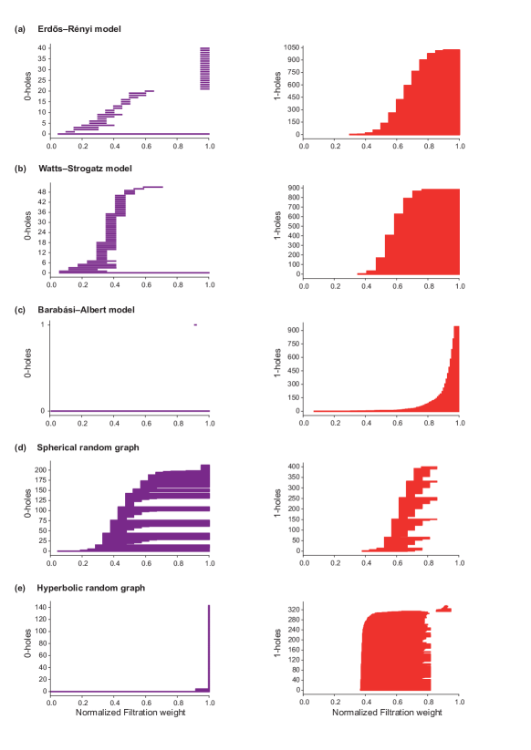
Figure 2: $H_{0}$ and $H_{1}$ barcode diagrams obtained using our new method based on Forman-Ricci curvature in model networks with average degree 4. (a) ER model with $n=1000$ and $p=0.004$. (b) WS model with $n=1000$, $k=4$ and $p=0.5$. (c) BA model with $n=1000$ and $m=2$. (d) Spherical random graphs produced from HGG model with $n=1000$, $T=0$, $k=4$ and $\gamma=\infty$. (e) Hyperbolic random graphs produced from HGG model with $n=1000$, $T=0$, $k=4$ and $\gamma=2$.

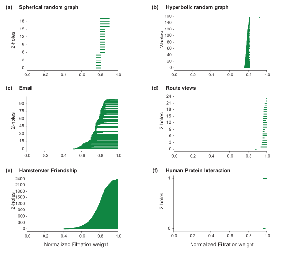
Figure 3: $H_{2}$ barcode diagrams obtained using our new method based on Forman-Ricci curvature in model and real networks. (a) Spherical random graph produced from HGG model with $n=1000$, $T=0$, $k=4$ and $\gamma=\infty$. (b) Hyperbolic random graph produced from HGG model with $n=1000$, $T=0$, $k=4$ and $\gamma=2$. (c) Email communication. (d) Route views. (e) Hamsterster friendship. (f) Human protein interaction.

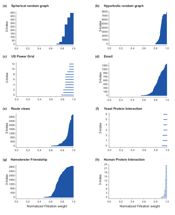
Figure 4: $H_{3}$ barcode diagrams obtained using our new method based on Forman-Ricci curvature in model and real networks. (a) Spherical random graph produced from HGG model with $n=1000$, $T=0$, $k=4$ and $\gamma=\infty$. (b) Hyperbolic random graph produced from HGG model with $n=1000$, $T=0$, $k=4$ and $\gamma=2$. (c) US Power Grid. (d) Email communication. (e) Route views. (f) Yeast protein interaction. (g) Hamsterster friendship. (h) Human protein interaction.

Figure 5: Bottleneck distance between persistence diagrams obtained using our new method based on Forman-Ricci curvature in model networks with average degree 4. For each of the five model networks, 10 random samples are generated by fixing the number of vertices $n$ and other parameters of the model. We report the distance (rounded to two decimal places) between two different models as the average of the distance between each of the possible pairs of the 10 sample networks corresponding to the two models along with the standard error.

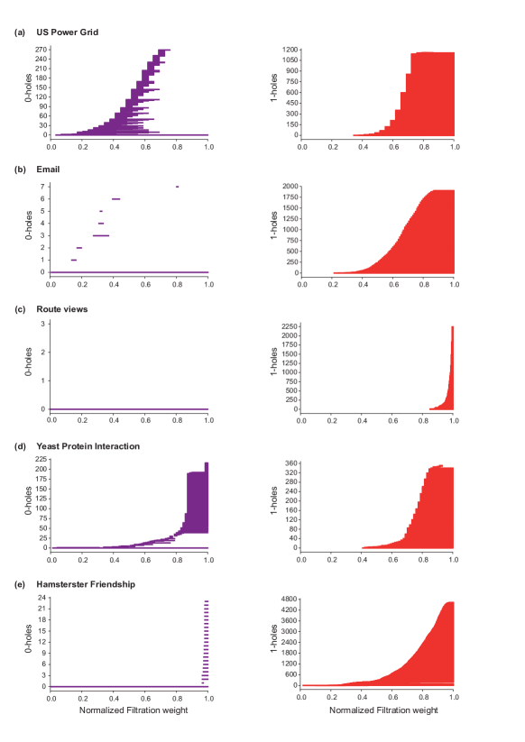
Figure 6: $H_{0}$ and $H_{1}$ barcode diagrams obtained using our new method based on Forman-Ricci curvature in real networks. (a) US Power Grid. (b) Email communication. (c) Route views. (d) Yeast protein interaction. (e) Hamsterster friendship.

4 Results and Discussion

4.1 Persistent homology of unweighted networks using Forman-Ricci curvature

We here present a new method based on Forman-Ricci curvature Sreejith et al. (2016, 2017); Samal et al. (2018) to study persistent homology in unweighted and undirected networks. Essentially, our method relies on transforming an unweighted and undirected graph $G$ into an edge-weighted network followed by construction of a weighted clique simplicial complex $K$.

We begin by transforming a given unweighted and undirected network into an edge-weighted network by assigning weights to edges based on their Forman-Ricci curvature (Figure 1). The Forman-Ricci curvature of each edge in an unweighted network can be computed using Equation 6 as described in the Theory section. Thereafter, we assign weights to edges in the network by normalization of the associated Forman-Ricci curvatures using the following formula:

$$w(e)=\frac{\rm{F}(e)-(\rm{F}_{\text{min}}-\epsilon)}{(\rm{F}_{\text{max}}+\epsilon)-(\rm{F}_{\text{min}}-\epsilon)}$$ (8)

where $w(e)$ is the weight of edge $e$, $\rm{F}(e)$ is the Forman-Ricci curvature of edge $e$, $\rm{F}_{\text{min}}$ and $\rm{F}_{\text{max}}$ are the minimum value and maximum value, respectively, of the Forman-Ricci curvature across all edges in the network, and $\epsilon$ is a positive number which is taken here to be 1. In sum, the above formula gives the weights of edges in the weighted network corresponding to the given unweighted and undirected network. In schematic Figure 1, we show this transformation of an unweighted and undirected graph into an edge-weighted network using an example.

Next, we construct a weighted clique simplicial complex starting from the edge-weighted network as follows (Figure 1). The $1$-simplices or edges in the clique complex corresponding to the edge-weighted network already have normalized weights based on their Forman-Ricci curvature. Based on the weights of $1$-simplices or edges, we assign weights to $0$-simplices or vertices such that the weight of a vertex in the clique complex is equal to the minimum of the weights of edges incident on the vertex (Equation 5). In other words, the weight of the $0$-simplex is the minimum of the weights of its $1$-dimensional co-faces in the clique complex. Similarly, we assign weights to $2$-simplices such that the weight of a $2$-simplex in the clique complex is equal to the maximum of the weights of its $1$-dimensional faces or edges (Equation 5). In the same manner, we can assign weights to higher-dimensional simplices (see Theory section). For example, the weight of a $3$-simplex in the clique complex is equal to the maximum of the weights of its $2$-dimensional faces. In schematic Figure 1, we show this construction of a weighted clique simplicial complex starting from an edge-weighted network using an example.

To construct a weighted clique simplicial complex corresponding to an unweighted and undirected network, our scheme hinges on assignment of weights to $0$-simplices (vertices) based on weights of their $1$-dimensional co-faces (i.e., edges attached to vertices). In many real-world networks, there are isolated vertices which are not attached to any edges in the graph. In our scheme, isolated vertices ($0$-simplices) are assigned weights equal to the maximum of the weights given to any simplex in the clique complex. In the example shown in schematic Figure 1, we assign weight to the isolated vertex $v_{9}$ in the weighted clique complex as described above.

After constructing the weighted clique complex $K$ corresponding to a given unweighted and undirected graph $G$, we investigate the persistent homology of the simplicial complex via the associated filtration described in Equation 4 in the Theory section. In order to construct this filtration of the weighted clique complex $K$, the assigned weights $w(\alpha_{i})$ to simplices $\alpha_{i}$ in $K$ are arranged in an increasing order, say $\lambda_{1}\leq\lambda_{2}\leq\cdots\leq\lambda_{n}$, and thereafter, the sequence of subcomplexes, $K(\lambda_{1})\subseteq K(\lambda_{2})\subseteq\cdots\subseteq K(\lambda_{n})$ is used to compute the persistent homology groups of $K$ as described in the Theory section. In schematic Figure 1, we show this filtration of the weighted clique complex corresponding to an unweighted and undirected network using an example.

In previous work Sreejith et al. (2016, 2017); Samal et al. (2018), it was shown that edges critical for the robustness of a complex network have highly negative Forman-Ricci curvature. From Equation 8, it follows that the assigned weights to edges or $1$-simplices in the weighted clique complex $K$ constructed by our scheme is likely to be inversely proportional to their importance from robustness perspective. Noteworthy, critical edges for the integrity of the network are likely to be added in the initial stages of the filtration of the weighted clique complex $K$, and thus, our method for studying the persistent homology revolves around the central idea that the more important features of the network are included in the initial stages of filtration.

We emphasize that the proposed method summarized in Figure 1 to study persistent homology in unweighted networks basically relies on transforming an unweighted network into an edge-weighted graph which is then used to construct a weighted clique complex. In principle, an edge-weighted graph can be obtained from an unweighted graph by assigning weights to edges based on any edge-centric measure. In our method summarized in Figure 1, we have chosen the edge-centric measure, Forman-Ricci curvature, for this transformation. Another possible and attractive choice of an edge-centric measure for this transformation is the edge betweenness centrality Freeman (1977); Girvan and Newman (2002); Newman (2010).

In this work, we have also explored this alternate choice of edge betweenness centrality to construct edge-weighted networks and study the persistent homology of unweighted networks. The edge betweenness centrality of an edge in an unweighted network can be computed using Equation 7 as described in the Theory section. Thereafter, we can assign weights to edges in the network by normalization of the associated edge betweenness centralities using the following formula:

$$w(e)=\frac{(\rm{EBC}_{\text{max}}+\epsilon)-\rm{EBC}(e)}{(\rm{EBC}_{\text{max}}+\epsilon)-(\rm{EBC}_{\text{min}}-\epsilon)}$$ (9)

where $w(e)$ is the weight of edge $e$, $\rm{EBC}(e)$ is the edge betweenness centrality of edge $e$, $\rm{EBC}_{\text{min}}$ and $\rm{EBC}_{\text{max}}$ are the minimum value and maximum value, respectively, of the edge betweenness centrality across all edges in the network, and $\epsilon$ is a positive number which is taken here to be 1. Since the edges with high edge betweenness centrality are highly critical for information flow in the network, the above equation assigns lower weights to such critical edges to ensure their addition during initial stages of the filtration.

In the main text of this paper, we report results from the investigation of persistent homology in unweighted networks using our method based on Forman-Ricci curvature. In the supplementary information (SI) of this paper, we report results from the investigation of persistent homology in unweighted networks using our method based on alternate choice of edge betweenness centrality. In the sequel, we will show that the qualitative and quantitative results obtained in unweighted model and real networks using our method based on Forman-Ricci curvature is very similar to our method based on edge betweenness centrality. However, the calculation of edge betweenness centrality requires computing all shortest paths between every distinct pair of vertices in the network, and thus, it is much more computationally expensive than Forman-Ricci curvature. Therefore, our method based on Forman-Ricci curvature is a better choice from a computational perspective to study persistent homology in unweighted and undirected networks.

4.2 Implementation in model and real networks

In this work, we have investigated five model networks and seven real-world networks using our methods based on Forman-Ricci curvature and edge betweenness centrality described in the preceding section to study persistent homology in unweighted and undirected networks.

For a given unweighted and undirected network $G$, either model or real-world, we first construct the corresponding edge-weighted network based on Forman-Ricci curvature (Equation 8) or edge betweenness centrality (Equation 9); thereafter, we construct a weighted clique simplicial complex $K$ and then study the corresponding filtration based on the edge weights as described in the preceding section. We remark that our investigation of the persistent homology in model and real networks is limited to the $3$-dimensional clique simplicial complex $K$ corresponding to $G$. That is, we only include $p$-simplices which have $0\leq p\leq 3$ while constructing the weighted clique simplicial complex $K$ starting from an unweighted graph $G$. For these computations of persistent homology in model and real networks, we use GUDHI Maria et al. (2014) which is a C++ based library for Topological Data Analysis (http://gudhi.gforge.inria.fr/).

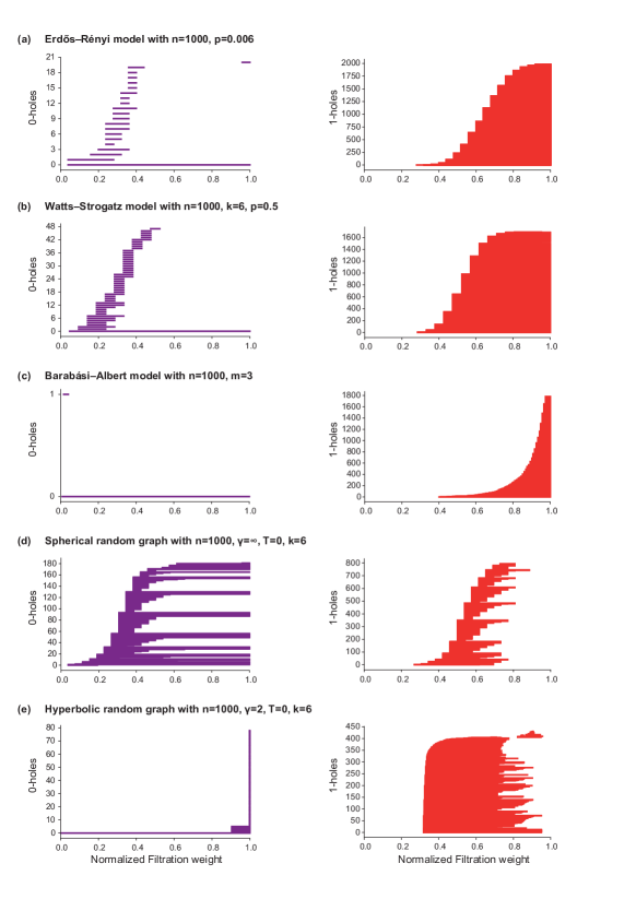
Figure S1: $H_{0}$ and $H_{1}$ barcode diagrams obtained using our new method based on Forman-Ricci curvature in model networks with average degree 6.

In the following, we present our results from application of our method based on Forman-Ricci curvature to study persistent homology in model and real networks (Figure 1). We have studied here five different model networks, namely, ER, WS, BA, spherical random graphs and hyperbolic random graphs (see Datasets section). The $0$-holes or $H_{0}$ barcode diagram gives the number of connected components in the network at every stage of the filtration. We find that the ER and WS networks possess a large number of components throughout the filtration in comparison to BA networks where there is typically a single component which persists across the entire filtration (Figure 2, SI Figures S1 and S2). This suggests that the simplices which are critical for the overall connectivity of the network are introduced during the initial stages of the filtration of BA networks in contrast to ER and WS networks. The $H_{1}$ barcode diagram indicates the presence of $1$-holes in the network. We find that the $1$-holes appear earlier during filtration in ER and WS networks in comparison to BA networks where $1$-holes appear towards the end of filtration (Figure 2, SI Figures S1 and S2). Thus, the $H_{0}$ and $H_{1}$ barcode diagrams are able to qualitatively distinguish scale-free BA networks from random ER networks and small-world WS networks (Figure 2, SI Figures S1 and S2). Lastly, $H_{2}$ and $H_{3}$ barcode diagrams do not provide any insight into the structure of ER, WS and BA networks due to the lack of $2$-holes and $3$-holes.

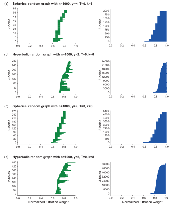
Figure S3: $H_{2}$ and $H_{3}$ barcode diagrams obtained using our new method based on Forman-Ricci curvature in model networks with average degree 6 and 8.

The ER, WS and BA networks can be distinguished from both spherical and hyperbolic random graphs based on significantly larger number of $0$-holes or connected components in the later (Figure 2, SI Figures S1 and S2). Though the number of components in the spherical and hyperbolic random graphs are similar, the patterns of filtration sequence is a distinguishing factor. The $0$-holes in the spherical random graph are more distributed across the filtration sequence, while there are very few $0$-holes in the hyperbolic random graph for most part of the filtration with the introduction of a large number of $0$-holes just before the end of the filtration. This can be understood by the presence of many isolated vertices in the hyperbolic random graphs which are assigned maximum weight in the corresponding weighted clique complex, and thus, appear at the end of filtration (Figure 2, SI Figures S1 and S2). Moreover, $1$-holes and $2$-holes appear during intermediate stages of filtration in both spherical and hyperbolic random graphs, however, these holes do not persist till the end of filtration (Figures 2-3, SI Figures S1-S3). Noteworthy, there are many more $3$-holes in hyperbolic random graphs in comparison to spherical graphs (Figure 4, SI Figure S3). Overall, these features enable qualitative distinction between hyperbolic and spherical model graphs with very different underlying geometry.

The barcode diagrams for the five model networks obtained from our method based on Forman-Ricci curvature can be used to make a qualitative distinction between different types of networks (Figure 2-4, SI Figures S1-S3). For a quantitative distinction between the topological features of the five model networks, we use the bottleneck distance between total persistence diagrams obtained from our method based on Forman-Ricci curvature as described in the Theory section. From Figure 5, it is seen that the bottleneck distance between BA and ER or WS networks of similar average degree is higher than the distance between ER and WS networks. Furthermore, the bottleneck distance is high between spherical and hyperbolic random graphs of similar average degree. Overall, the bottleneck distances between the total persistence diagrams for the five model networks provide a quantitative validation of the applicability of our method based on Forman-Ricci curvature to reveal distinct topological features in unweighted and undirected networks.

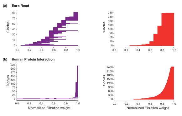
Figure S4: $H_{0}$ and $H_{1}$ barcode diagrams obtained using our new method based on Forman-Ricci curvature in real networks. (a) Euro road. (b) Human protein interaction.

We have also studied here seven well-known real-world networks (see Datasets section). From the $H_{0}$ barcode of the US Power Grid network, it is clear that there is one connected component which persists across the entire filtration despite many transient components appearing and disappearing during intermediate stages of filtration (Figure 6). The $H_{0}$ barcode diagrams of the E-mail and Route views networks are similar in the sense that the number of connected components across the entire filtration is low (Figure 6). The $H_{0}$ barcode diagrams of the two biological networks, namely Human protein interaction and Yeast protein interaction show a sudden increase in the number of connected components at the final stage of filtration (Figure 6, SI Figure S4). The $H_{0}$ barcode diagram of the Euro road network displays a distributed pattern with components spanning across varied intervals of filtration (SI Figure S4). The $H_{1}$ barcode diagrams of the seven real networks are similar in the respect that there is typically an increase in the number of $1$-holes around the middle to later stages of filtration (Figure 6, SI Figure S4). We also display the $H_{2}$ and $H_{3}$ barcode diagrams for real networks in Figures 3 and 4, respectively. Note that the Euro road network is devoid of $2$-holes and $3$-holes, while the Yeast protein interaction network and US Power Grid network are devoid or $2$-holes (Figures 3 and 4). In sum, the barcode diagrams obtained using our method based on Forman-Ricci curvature can be used to reveal differences between model and real networks.

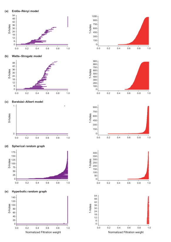
Figure S5: $H_{0}$ and $H_{1}$ barcode diagrams obtained using our new method based on edge betweenness centrality in model networks with average degree 4.

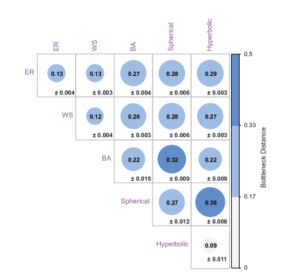
Figure S10: Bottleneck distance between persistence diagrams obtained using our new method based on edge betweenness centrality in model networks with average degree 4. For each of the five model networks, 10 random samples are generated by fixing the number of vertices $n$ and other parameters of the model. We report the distance (rounded to two decimal places) between two different models as the average of the distance between each of the possible pairs of the 10 sample networks corresponding to the two models along with the standard error.

In the above paragraphs, we reported our results from application of our method based on Forman-Ricci curvature to study persistent homology in unweighted networks, both model and real-world. As described in the preceding section, we can also apply an alternate method based on edge betweenness centrality to study persistent homology in unweighted networks, both model and real-world. In SI Figures S5-S9, we present the $H_{0}$, $H_{1}$, $H_{2}$ and $H_{3}$ barcode diagrams obtained using our alternate method based on edge betweenness centrality in five model and seven real-world networks. Based on SI Figures S5-S9, it is evident that we are also able to make qualitative distinction between varied model networks using the barcode diagrams obtained from our method based on edge betweenness centrality, and these results are similar to results described above from our method based on Forman-Ricci curvature. Moreover, in SI Figure S10, we display the bottleneck distances between persistence diagrams corresponding to the five model networks obtained using the alternate method based on edge betweenness centrality, and these results are also similar to those shown in Figure 5 which are obtained using our method based on Forman-Ricci curvature.

4.3 Comparison with method based on discrete Morse theory

Classical Morse theory on smooth manifolds has been a rich theory to detect the topology of the underlying space Morse (1934). However, it requires a smooth structure to probe the topology via real-valued smooth functions. Robin Forman introduced discrete Morse theory, the discrete counterpart of classical Morse theory Forman (1998, 2002), which is applicable to a large class of topological objects called $CW$-complexes, even those which lack smoothness. Similar to classical Morse theory, this discretized version also captures the topology of the underlying object. A fundamental notion in discrete Morse theory is that of critical cells, which are the discrete analogues of equilibrium points of a Morse function, i.e. points on which its gradient vanishes. The number of such critical cells is intricately related to the Betti numbers and the Euler characteristic of the topological space via the Morse inequalities Forman (1998, 2002).

In our previous work Kannan et al. (2019), we have used discrete Morse theory of Robin Forman to set weights on the clique complex of an unweighted graph. We also gave an algorithm to produce a near-optimal discrete Morse function, in the sense that the number of so-called critical simplices of the function is close to the theoretical minimum given by Betti numbers. The advantages of this approach lies in the ability for preprocessing of the simplicial complex, which leads to significant simplification that in turn, leads to computational efficiency for homology calculations Mischaikow and Nanda (2013); Harker et al. (2014). In principle, one can use this method independent of TDA, for example to study combinatorial topology aspects of such complexes Shareshian (2001). As an application to TDA, we Kannan et al. (2019) used this method to compute the persistent homology of the model and real-world networks which are also analyzed in this contribution, and showed that it was able to distinguish between various networks with different topological features.

Our present method focusses on the computation of persistent homology only, setting aside the computational advantages of using a near-optimal discrete Morse function. We have shown that even though we lose the simplified topological structure provided by discrete Morse theory, we can still apply other weighting schemes using local and global measures like Forman-Ricci curvature and edge betweenness centrality, to compute persistent homology of various networks. Indeed, the new method also distinguishes the various model networks as well as the previous method using discrete Morse theory. Therefore, using these new weighting schemes can be seen as a tradeoff between computational efficiency and applicability of TDA to unweighted graphs.

5 Conclusions

This work is meant to provide techniques to apply TDA, for the investigation of topological properties of unweighted networks. We employ two methods to convert an unweighted network into a weighted network. The first one is a discretized version of Ricci curvature which takes into account only local information around an edge in the network, while the second one is a global quantifier which measures the importance of an edge based on the number of shortest paths between any two distinct vertices of the network passing through that edge. Once we have a weighted graph, standard techniques allow us to obtain a filtration of the associated clique complexes, and thereby compute their persistent homology (Figure 1). We have applied this method to study five different kinds of model networks. We also show that this method can distinguish different model networks via the averaged bottleneck distance between the corresponding persistence diagrams (Figure 5). We also apply the same techniques to study some well-known real-world networks to obtain insights into their underlying topology. In future work, we plan to apply these techniques to networks arising out of physical systems, with the goal of trying to find correlations between dynamics of such systems and their underlying topology via the application of TDA.

Funding

This work was supported by Max Planck Society, Germany, through the award of a Max Planck Partner Group in Mathematical Biology (to A.S.) and Science and Engineering Research Board (SERB), Department of Science and Technology (DST) India through the award of a MATRICS grant [MTR/2017/000835] (to I.R.).

Declaration of Competing Interest

None.

Acknowledgments

S.V. and S.J.R. thank the Institute of Mathematical Sciences (IMSc), Chennai, India for their local hospitality and R. Nadarajan for encouragement.

Author contributions

I.R. and A.S. designed the study and developed the method. S.V. and S.J.R. performed the simulations. I.R. and A.S. analyzed results. I.R., S.V., S.J.R. and A.S. wrote the manuscript. All authors reviewed and approved the manuscript.

SUPPLEMENTARY INFORMATION (SI)

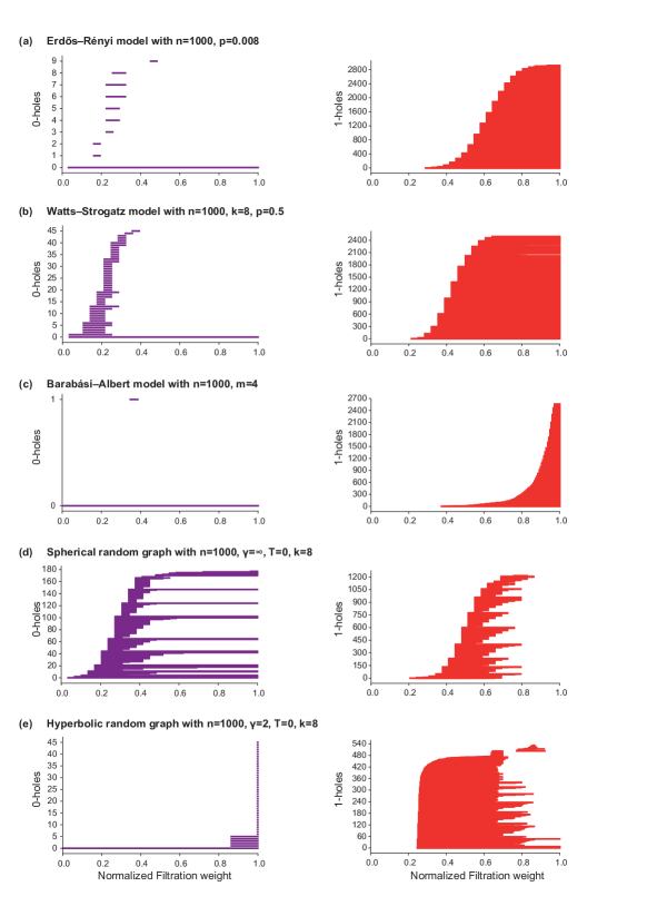
Figure S2: $H_{0}$ and $H_{1}$ barcode diagrams obtained using our new method based on Forman-Ricci curvature in model networks with average degree 8.

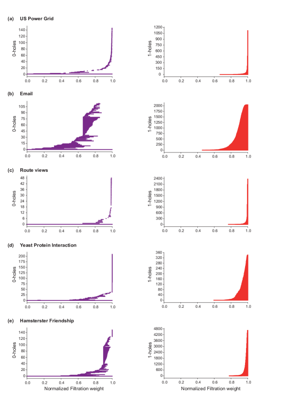
Figure S6: $H_{0}$ and $H_{1}$ barcode diagrams obtained using our new method based on edge betweenness centrality in real networks. (a) US Power Grid. (b) Email communication. (c) Route views. (d) Yeast protein interaction. (e) Hamsterster friendship.

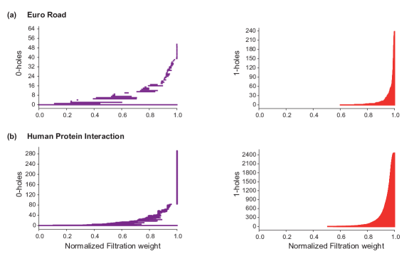
Figure S7: $H_{0}$ and $H_{1}$ barcode diagrams obtained using our new method based on edge betweenness centrality in real networks. (a) Euro road. (b) Human protein interaction.

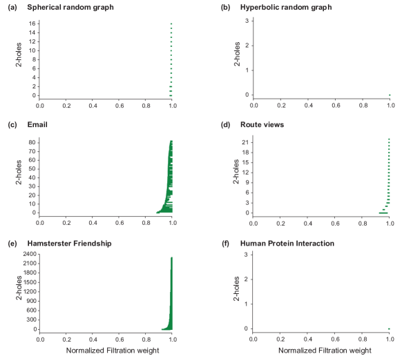
Figure S8: $H_{2}$ barcode diagrams obtained using our new method based on edge betweenness centrality in model and real networks. (a) Spherical random graph produced from HGG model with $n=1000$, $T=0$, $k=4$ and $\gamma=\infty$. (b) Hyperbolic random graph produced from HGG model with $n=1000$, $T=0$, $k=4$ and $\gamma=2$. (c) Email communication. (d) Route views. (e) Hamsterster friendship. (f) Human protein interaction.

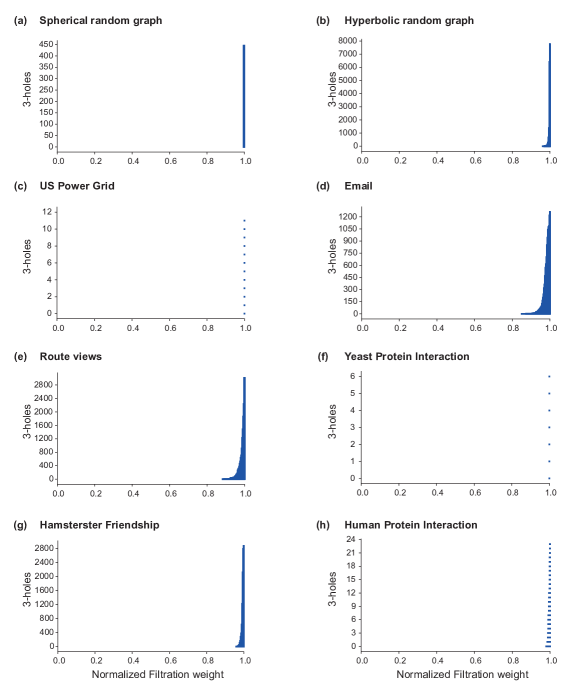
Figure S9: $H_{3}$ barcode diagrams obtained using our new method based on edge betweenness centrality in model and real networks. (a) Spherical random graph produced from HGG model with $n=1000$, $T=0$, $k=4$ and $\gamma=\infty$. (b) Hyperbolic random graph produced from HGG model with $n=1000$, $T=0$, $k=4$ and $\gamma=2$. (c) US Power Grid. (d) Email communication. (e) Route views. (f) Yeast protein interaction. (g) Hamsterster friendship. (h) Human protein interaction.

References

- Zomorodian and Carlsson (2005) A. Zomorodian and G. Carlsson, Discrete & Computational Geometry 33, 249 (2005).
- Edelsbrunner and Harer (2008) H. Edelsbrunner and J. Harer, Contemporary Mathematics 453, 257 (2008).
- Carlsson (2009) G. Carlsson, Bulletin of the American Mathematical Society 46, 255 (2009).
- Pranav et al. (2016) P. Pranav, H. Edelsbrunner, R. Van de Weygaert, G. Vegter, M. Kerber, B. Jones, and M. Wintraecken, Monthly Notices of the Royal Astronomical Society 465, 4281 (2016).
- Günther et al. (2011) D. Günther, J. Reininghaus, I. Hotz, and H. Wagner, in 2011 24th SIBGRAPI Conference on Graphics, Patterns and Images (IEEE, 2011) pp. 25–32.
- Nicolau et al. (2011) M. Nicolau, A. Levine, and G. Carlsson, Proceedings of the National Academy of Sciences USA 108, 7265 (2011).
- Rizvi et al. (2017) A. H. Rizvi, P. G. Camara, E. K. Kandror, T. J. Roberts, I. Schieren, T. Maniatis, and R. Rabadan, Nature Biotechnology 35, 551 (2017).
- Munkres (2018) J. Munkres, Elements of algebraic topology (CRC Press, 2018).
- Watts and Strogatz (1998) D. J. Watts and S. H. Strogatz, Nature 393, 440 (1998).
- Barabási and Albert (1999) A. L. Barabási and R. Albert, Science 286, 509 (1999).
- Albert and Barabási (2002) R. Albert and A. L. Barabási, Reviews of Modern Physics 74, 47 (2002).
- Newman (2010) M. E. J. Newman, Networks: An Introduction (Oxford University Press, 2010).
- Barabási (2016) A.-L. Barabási, Network Science (Cambridge University Press, 2016).
- Bollobas (1998) B. Bollobas, Modern Graph Theory (Springer, 1998).
- De Silva and Ghrist (2007) V. De Silva and R. Ghrist, Notices of the American mathematical society 54 (2007).
- Horak et al. (2009) D. Horak, S. Maletić, and M. Rajković, Journal of Statistical Mechanics: Theory and Experiment , P03034 (2009).
- Petri et al. (2013) G. Petri, M. Scolamiero, I. Donato, and F. Vaccarino, PloS One 8, e66506 (2013).
- Petri et al. (2014) G. Petri, P. Expert, F. Turkheimer, R. Carhart-Harris, D. Nutt, P. J. Hellyer, and F. Vaccarino, Journal of The Royal Society Interface 11, 20140873 (2014).
- Bianconi (2015) G. Bianconi, Europhysics Letters 111, 56001 (2015).
- Wu et al. (2015) Z. Wu, G. Menichetti, C. Rahmede, and G. Bianconi, Scientific Reports 5, 10073 (2015).
- Sizemore et al. (2016) A. Sizemore, C. Giusti, and D. Bassett, Journal of Complex Networks 5, 245 (2016).
- Courtney and Bianconi (2017) O. T. Courtney and G. Bianconi, Physical Review E 95, 062301 (2017).
- Ritchie et al. (2017) M. Ritchie, L. Berthouze, and I. Z. Kiss, Journal of complex networks 5, 1 (2017).
- Courtney and Bianconi (2018) O. T. Courtney and G. Bianconi, Physical Review E 97, 052303 (2018).
- Kartun-Giles and Bianconi (2019) A. P. Kartun-Giles and G. Bianconi, Chaos, Solitons & Fractals: X 1, 100004 (2019).
- Iacopini et al. (2019) I. Iacopini, G. Petri, A. Barrat, and V. Latora, Nature Communications 10, 2485 (2019).
- Kannan et al. (2019) H. Kannan, E. Saucan, I. Roy, and A. Samal, Scientific Reports 9, 13817 (2019).
- Klamt et al. (2009) S. Klamt, U. Haus, and F. Theis, PLoS Computational Biology 5, e1000385 (2009).
- Zlatić et al. (2009) V. Zlatić, G. Ghoshal, and G. Caldarelli, Physical Review E 80, 036118 (2009).
- Lee et al. (2012) H. Lee, H. Kang, M. Chung, B.-N. Kim, and D. Lee, IEEE transactions on medical imaging 31, 2267 (2012).
- Jeong et al. (2001) H. Jeong, S. P. Mason, A. L. Barabási, and Z. N. Oltvai, Nature 411, 41 (2001).
- Leskovec et al. (2007) J. Leskovec, J. Kleinberg, and C. Faloutsos, ACM Transactions on Knowledge Discovery from Data (TKDD) 1, 2 (2007).
- Šubelj and Bajec (2011) L. Šubelj and M. Bajec, European Physical Journal B 81, 353 (2011).
- Forman (1998) R. Forman, Advances in Mathematics 134, 90 (1998).
- Forman (2002) R. Forman, Sém. Lothar. Combin. 48, 1 (2002).
- Forman (2003) R. Forman, Discrete and Computational Geometry 29, 323 (2003).
- Sreejith et al. (2016) R. Sreejith, K. Mohanraj, J. Jost, E. Saucan, and A. Samal, Journal of Statistical Mechanics: Theory and Experiment , P063206 (2016).
- Sreejith et al. (2017) R. P. Sreejith, J. Jost, E. Saucan, and A. Samal, Chaos, Solitons & Fractals 101, 50 (2017).
- Samal et al. (2018) A. Samal, R. P. Sreejith, J. Gu, S. Liu, E. Saucan, and J. Jost, Scientific Reports 8, 8650 (2018).
- Freeman (1977) L. C. Freeman, Sociometry 40, 35 (1977).
- Girvan and Newman (2002) M. Girvan and M. Newman, Proceedings of the National Academy of Sciences USA 99, 7821 (2002).
- Ghrist (2008) R. Ghrist, Bulletin of the American Mathematical Society 45, 61 (2008).
- Di Fabio and Ferri (2015) B. Di Fabio and M. Ferri, in Image Analysis and Processing — ICIAP 2015, edited by V. Murino and E. Puppo (Springer International Publishing, Cham, 2015) pp. 294–305.
- Cohen-Steiner et al. (2007) D. Cohen-Steiner, H. Edelsbrunner, and J. Harer, Discrete & Computational Geometry 37, 103 (2007).
- Jost (2017) J. Jost, Riemannian Geometry and Geometric Analysis, 7th ed. (Springer International Publishing, 2017).
- Saucan et al. (2019) E. Saucan, R. P. Sreejith, R. P. Vivek-Ananth, J. Jost, and A. Samal, Chaos, Solitons & Fractals 118, 347 (2019).
- Erdös and Rényi (1961) P. Erdös and A. Rényi, Bull. Inst. Internat. Statist 38, 343 (1961).
- Krioukov et al. (2010) D. Krioukov, F. Papadopoulos, M. Kitsak, A. Vahdat, and M. Boguná, Physical Review E 82, 036106 (2010).
- Rual et al. (2005) J. F. Rual, K. Venkatesan, T. Hao, T. Hirozane-Kishikawa, A. Dricot, N. Li, G. F. Berriz, F. D. Gibbons, M. Dreze, N. Ayivi-Guedehoussou, and et al, Nature 437, 1173 (2005).
- Guimera et al. (2003) R. Guimera, L. Danon, A. Diaz-Guilera, F. Giralt, and A. Arenas, Physical Review E 68, 065103 (2003).
- Kunegis (2013) J. Kunegis, in Proceedings of the 22nd International Conference on World Wide Web companion (ACM, New York, NY, USA, 2013) pp. 1343–1350.
- Maria et al. (2014) C. Maria, J.-D. Boissonnat, M. Glisse, and M. Yvinec, in International Congress on Mathematical Software (Springer, 2014) pp. 167–174.
- Morse (1934) M. Morse, The calculus of variations in the large, Vol. 18 (American Mathematical Society, 1934).
- Mischaikow and Nanda (2013) K. Mischaikow and V. Nanda, Discrete & Computational Geometry 50, 330 (2013).
- Harker et al. (2014) S. Harker, K. Mischaikow, M. Mrozek, and V. Nanda, Foundations of Computational Mathematics 14, 151 (2014).
- Shareshian (2001) J. Shareshian, Topology 40, 681 (2001).