Hypercubic cluster states in the phase modulated quantum optical frequency comb

Abstract

We propose and fully analyze the simplest technique to date to generate light-based universal quantum computing resources, namely 2D, 3D and, in general, $n$-hypercubic cluster states. The technique uses two standard optical components: first, a single optical parametric oscillator pumped below threshold by a monochromatic field, which generates Einstein-Podolsky-Rosen entangled states, a.k.a. two-mode-squeezed states, over the quantum optical frequency comb; second, phase modulation at frequencies multiple of the comb spacing (via RF or optical means). The unprecedented compactness of this technique paves the way to implementing quantum computing on chip using quantum nanophotonics.

Introduction. For quantum information technology to become a reality, quantum engineering must come of age. A promising approach is quantum photonics, marrying fundamental quantum optics with integrated photonics. On the fundamental side, quantum optics provides a scalable platform for continuous-variable (CV) universal quantum computing (QC), based on qumodes (e.g. quantum optical fields) rather than qubits  [1, 2, 3, 4, 5], as has been based demonstrated with temporal or spectral phase-locked quantum optical combs, emitted by optical parametric oscillators (OPOs). The interference of shifted, two-mode-squeezed quantum optical combs has been shown to yield cluster states [6, 7], which are universal quantum computing resources [8, 3], in the spectral domain [9, 10, 11] and in the temporal domain [12, 13, 14, 15], with thousands to millions of entangled qumodes. Other schemes, based on the spatial degrees of freedom have been been accomplished [16] or proposed [17, 18]. It is important to note that CVQC can be made fault tolerant at reachable squeezing levels [19, 20].

Most of the aforementioned work in the temporal and spectral domains relied on interfering two to four straddling squeezed quantum combs, as originally proposed in Refs. 21 and also 22. In this paper, we show that a single comb is in fact sufficient to generate $n$-hypercubic cluster states of arbitrary dimension $n$. Such states are universal resources for quantum computing for $n=2$ [8], For $n=3$, they can also allow quantum error correction topological encoding [23].

Our implementation uses the spectral domain, i.e., the quantum optical frequency comb (QOFC) emitted by a single OPO that is phase modulated by a sparse discrete spectrum (either inside or outside of the OPO cavity). Remarkably, the dimension of the cluster graph is determined by the number of modulation frequencies and its size is determined by their spacing.

This discovery was made possible by a general analysis of the generated Gaussian graph state, factoring in concrete experimental parameters such as finite squeezing, pump amplitude, and modulation depth [25]. Our results account for all graph errors and allow us to drastically simplify experimental configurations, paving the way to compact realizations of large-scale cluster entanglement using a single OPO on chip [26, 27, 28, 29, 30].

The paper is organized as follows. In Section I, we recall the quantum description of phase modulation and outline the derivation of the quantum state obtained for a two-mode-squeezed input. In Section II, we present our theoretical results and show that a single phase-modulated OPO can generate precisely defined, $n$-hypercubic cluster states. In Section III we thoroughly analyze graph errors and the full effects of finite squeezing. We then conclude.

I Phase modulation of Gaussian states

I.1 Quantum optical phase modulation

Phase modulation (PM) at frequency $\Omega$ of a monochromatic carrier field of frequency $\omega_{o}$ creates harmonic sidebands at frequencies $\omega_{\scriptscriptstyle n}=\omega_{\scriptscriptstyle o}+n\Omega$ ($n\in\mathbb{Z}$) and of amplitudes the Bessel functions of the first kind

$$e^{i[\omega_{o}t+m\sin(\Omega t+\phi)]}=e^{i\omega_{o}t}\sum_{n=-\infty}^{\infty}J_{n}(m)\,e^{in(\Omega t+\phi)},$$ (1)

where $m$ is the modulation index and $\phi$ the PM phase. An effective quantum model of PM [31] is the multiport frequency-domain beamsplitter (Fig.1)

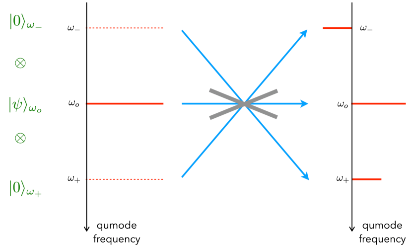
Figure 1: Quantum model of phase modulation at frequency $\Omega$ by a 3$\times$3 frequency-domain beamsplitter, Eq. (2) [31], symbolized by the unphysical gray element that features two frequency-domain “reflective,” and one “transmissive,” possibilities for each input beam (blue lines) at $\omega_{\scriptscriptstyle\pm}$=$\omega_{\scriptscriptstyle o}$$\pm$$\Omega$. For simplicity, we didn’t draw modulation sidebands of order greater than 1. An arbitrary input state is given in green, containing 3 qumodes (red lines) indexed by their frequency. A key point is that the carrier qumode at $\omega_{o}$ is coupled by PM to the input vacuum modes. When $\left|\,\psi\,\right\rangle$ is a coherent state, the output remains a product of coherent states.

Hamiltonian

$$H_{\textit{PM}}=\hbar\frac{\alpha}{\tau}e^{-i\phi}\sum_{j=-\infty}^{\infty}a_{j}a_{j+\Omega}^{\dagger}+\text{H.c.},$$ (2)

where $\alpha=m/2$, $\tau$ is the interaction time in the phase modulator, and $a_{j}$ is the annihilation operator of the qumode of frequency $j$ in units of the qumode spacing, i.e., of the free spectral range (FSR) of the OPO. We take $\Omega$ in units of the FSR from Eq. (2) on. Unitarity of quantum mechanics requiring there be as many input ports as there are output ports, PM of a single qumode will feature vacuum contamination at the sideband frequencies $\omega_{\pm}$, Fig.1. Such inputs are undesirable as random vacuum fluctuations decorrelate squeezed and entangled quantum states.

The use of a QOFC input to PM replaces vacuum inputs with QOFC qumodes when $\Omega$ is an integer, Fig.2. Throughout this paper the input state will be a two-mode squeezed QOFC generated by a monochromatically pumped, below-threshold OPO of Hamiltonian

$$H_{\textit{TMS}}=i\hbar\frac{r}{\tau^{\prime}}\sum_{j=1}^{N}a^{{\dagger}}_{j}a^{{\dagger}}_{p-j}+\text{H.c.},$$ (3)

where $p$ is the pump frequency in FSR units, $r$ is the squeezing parameter and $\tau^{\prime}$ approximates the OPO cavity lifetime. This Hamiltonian generates two-mode squeezing [33] between qumodes $j$ and $p$-$j$, thereby creating an arbitrarily good approximation of an EPR pair [34].

In Section II, we derive the $N$-qumode quantum state created by two different quantum evolutions: first, by an externally modulated OPO, for which the output state is

$$\left|\,\text{out}\,\right\rangle=\exp(-\tfrac{i\tau}{\hbar}H_{\textit{PM}})\exp(-\tfrac{i\tau^{\prime}}{\hbar}H_{\textit{TMS}})\left|\,0\,\right\rangle^{\otimes^{N}},$$ (4)

second, by an intrinsically phase-modulated OPO (e.g. with intracavity electro-optic modulation—EOM), described by

$$\left|\,\text{out}\,\right\rangle=\exp[-\tfrac{i\tau^{\prime}}{\hbar}(H_{\textit{TMS}}+H_{\textit{PM}})]\left|\,0\,\right\rangle^{\otimes^{N}}.$$ (5)

One final word about the Hamiltonians of Eqs. (2) & (3): we took the number of qumodes to be infinite in the former and finite in the latter, taking into account the phasematching bandwidth. This raises the question of qumodes at the edge of the phasematching bandwidth being coupled to vacuum modes which will degrade the entanglement. In addition, the edge of the phasematching bandwidth isn’t sharp from one mode to its nearest neighbor so we can expect some variations of the entanglement in that region. While these concerns are legitimate, the resulting graph imperfections will remain confined to the boundary of the cluster state, due to its local nature, i.e. the ends of a 1D chain, the perimeter of a 2D graph, and the enveloping area of a 3D graph. Since, for cluster states, any local imperfections can be removed by single-qubit/qumode measurements [6, 7, 35], these defects can be efficiently erased compared to the computation requirements which involve measurements of the bulk of the graph. We now outline the derivation procedure.

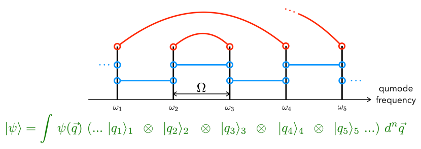
Figure 2: Quantum description of PM at frequency $\Omega$ (blue lines) of the two-mode-squeezed (red lines, pump frequency $\omega_{\scriptscriptstyle 2}+\omega_{\scriptscriptstyle 3}$) QOFC: because the modulation frequency equals the qumode spacing, there is no vacuum input and a unitary operation can be realized solely on the initial comb state $\left|\,\psi\,\right\rangle$.

I.2 Output state derivation

We proceed in three steps: first, deriving the symplectic matrix $\bf S$ of the quantum evolution in the Heisenberg picture, second, deducing from it the covariance matrix $\mathbf{\Sigma}$ of the state, third, obtaining the adjacency matrix $\bf V$ and error matrix $\bf U$ of the corresponding graph state. An additional fourth step is warranted in the case of cascaded Hamiltonians, Eq. (4), which employs a Möbius transformation.

I.2.1 Quantum evolution and covariance matrix

Any $N$-mode Gaussian Hamiltonian (i.e., quadratic in the field variables, we ignore displacements) yields a linear system of Heisenberg equations

$$\frac{d\mathbf{x}}{dt}=\mathbf{G}\mathbf{x},$$ (6)

where $\bf G$ is a symmetric matrix and where we posed x=$({\bf Q},{\bf P})^{T}$, Q=$(Q_{1},...,Q_{N})^{T}$, P=$(P_{1},...,P_{N})^{T}$. Equation (6) can be solved by diagonalizing $\mathbf{G}=\mathbf{R}\mathbf{G}_{\text{diag}}\mathbf{R}^{-1}$, yielding the solution

$${\bf x}(\tau)=\mathbf{S}\,{\bf x}(0),$$ (7)

where the symplectic matrix $\mathbf{S}$ is given by

$$\mathbf{S}=\mathbf{R}\,e^{\tau\mathbf{G}_{\text{diag}}}\,\mathbf{R}^{-1}.$$ (8)

Note that, in a sequence of unitary operations, the symplectic matrix ordering is the Schrödinger picture one

$${\mathbf{x}}(\tau_{n})={\mathbf{S}_{n}}{\mathbf{S}_{n-1}}\cdot\cdot\cdot{\mathbf{S}_{1}}{\mathbf{x}}(0)={\mathbf{S}}{\mathbf{x}}(0).$$ (9)

Once $\mathbf{S}$ is known, we obtain the covariance matrix $\mathbf{\Sigma}$, which contains all information about the Gaussian state,

$$\mathbf{\Sigma}=\frac{1}{2}\,\mathbf{S}\mathbf{S}^{T}.$$ (10)

An important property of $\mathbf{\Sigma}$ is that it is related to the complex graph of the Gaussian state [36], which we now briefly introduce.

Reminders on graph and cluster states

A qubit graph state is canonically defined the following way [6, 37]: graph vertices $j$ denote qubits in state $\left|\,+\,\right\rangle_{j}=(\left|\,0\,\right\rangle_{j}+\left|\,1\,\right\rangle_{j})/\sqrt{2}$ and graph edges $(j,k)$ denote controlled $Z$ gates $\text{CZ}_{jk}$. The stabilizers of a graph state—the operators that leave the state unchanged—form a group of Pauli generators $X_{j}\bigotimes_{k\in\mathbf{N}_{j}}Z_{k}$, where $j$=1,…,$N$ denotes each graph vertex and $\mathbf{N}_{j}$ is the neighborhood of $j$, i.e., the set of all vertices sharing an edge with $j$. A graph state can have any graph but the term “cluster state” is usually reserved for graph states that are sparse enough to allow measurement-based quantum computing [38, 39, 40]. In this paper, we use the “cluster state” moniker as the states we propose to generate are all sparse and adequate for one-way QC.

The exact analogues of qubit graph states for CV quantum information are well defined [7, 35, 1]. A Gaussian cluster state is composed of vertices $j$ denoting phase-squeezed states $S_{j}(r)\left|\,0\,\right\rangle_{j}=e^{\frac{r}{2}(a_{j}^{{\dagger}2}-a_{j}^{2})}\left|\,0\,\right\rangle_{j},$ where $r$ is the squeezing parameter. Here “phase” pertains to the phase quadrature $P=(a-a^{\dagger})/(i\sqrt{2})$. The edges $(j,k)$ of the cluster state graph denote the quantum nondemolition [41] controlled-phase interaction $\exp(iQ_{j}Q_{k})$, where $Q=(a+a^{\dagger})/\sqrt{2}$ is the field amplitude quadrature. In the limit of infinite squeezing, the CV graph state stabilizers are the generators of the Weyl-Heisenberg displacement group, e.g.  $e^{-iP_{j}}\bigotimes_{k\in\mathbf{N}_{j}}e^{iQ_{k}}$. This leads to the equivalent definition of operators that multiply the state by 0, a.k.a. nullifiers: $P_{j}-\sum_{k\in\mathbf{N}_{j}}Q_{k}$. Finally, note that fault-tolerant QC is theoretically possible for finitely squeezed Gaussian states [19].

I.2.2 Derivation of the Gaussian state graph

A qubit graph state is described by an unweighted adjacency matrix whose entries denote edge presence (value 1) or absence (value 0). Gaussian states are described by a complex-weighted  adjacency matrix $\mathbf{Z}=\mathbf{V}+i\mathbf{U}$, where V is the exact analog to the adjacency matrix of a qubit graph state [1] and U is the error matrix, which will be discussed in detail in Section III.

Any Gaussian state $\left|\,\psi\,\right\rangle$ can be defined by its nullifying operators, or nullifiers

$$({\bf P}-{\bf Z}{\bf Q})\left|\,\psi\,\right\rangle=\mathbf{0}\left|\,\psi\,\right\rangle,$$ (11)

which are, obviously, the logarithms of the stabilizers of $\left|\,\psi\,\right\rangle$. Because $\bf Z$ is complex in general, these nullifiers are non-Hermitian and cannot be measured, which makes measurement-based quantum computing problematic since it must proceed by measuring, among other things, graph nullifiers [35]. Thus, only Gaussian states with $\bf Z$ real, i.e. with $\bf Z$=$\bf V$ and $\bf U$=$\mathbf{0}$, can be proper cluster states.

However, measurement-based quantum computing is still possible with $\bf U$$\neq$$\mathbf{0}$. In that case, we use the (arbitrarily good) approximate nullifiers given by Hermitian operators ${\bf P}-{\bf V}{\bf Q}$, which verify [36]

$${\rm cov}[{\bf P}-{\bf V}{\bf Q}] =\frac{1}{2}\,{\bf U},$$ (12)

where we defined the covariance matrix in the standard way for vector operator $\bf A$ with zero expectation values in state $\left|\,\psi\,\right\rangle$,

$$({\rm cov}[\mathbf{A}])_{jk}=\frac{1}{2}\left\langle\,\psi\,\right|\{A_{j}^{\dagger},A_{k}\}\left|\,\psi\,\right\rangle.$$ (13)

We can deduce from Eq. (12) that an arbitrary Gaussian state of matrix $\bf Z$ can be accurately considered as a cluster state of matrix $\bf V$ iff

(i), the error matrix U is diagonal [25] and,

(ii), it verifies ${\rm Tr}[\mathbf{U}]\to 0$ in the limit of infinite squeezing [36].

In that case, $\mathbf{P}-\bf VQ$ are squeezed, uncorrelated Hermitian operators. Proper examination of $\bf U$ in light of requirements (i,ii) is therefore crucial and will be presented in Section III.

We are now ready to determine the Gaussian graph matrix $\bf Z$ from the covariance matrix. The relation between the two is [36]

$$\mathbf{\Sigma}_{x}={\rm cov}[\mathbf{x}]=\frac{1}{2}\begin{pmatrix}\mathbf{U}^{-1}&\mathbf{U}^{-1}\mathbf{V}\\ \mathbf{V}\mathbf{U}^{-1}&\mathbf{U}+\mathbf{V}\mathbf{U}^{-1}\mathbf{V}\end{pmatrix},$$ (14)

where the block structure coïncides with the definition of x. One final remark highlights the importance of $\bf U$. The covariance matrix can be rewritten, using the rewritten symplectic vector $\mathbf{y}=(\mathbf{Q},\mathbf{P}-\mathbf{V}\mathbf{Q})^{T}$, as

$$\mathbf{\Sigma}_{y}={\rm cov}[\mathbf{y}]=\frac{1}{2}\begin{pmatrix}\mathbf{U}^{-1}&\mathbb{O}\\ \mathbb{O}&\mathbf{U}\end{pmatrix}.$$ (15)

An allowable strategy for diagonalizing U so that it verifies (i,ii) above is to apply local symplectic operations, which are equivalent to local unitaries (LU), to qumodes [36, 25] since these cannot change the state’s entanglement. We will be making abundant use of this property.

I.2.3 Derivation of the graph for cascaded Hamiltonians [Eq. (4)]

As mentioned in Section I.1, we will consider PM either external or intrinsic to the OPO. Both options can be tackled using the procedure outlined above, with the former, cascading option making use of Eq. (9). Another, equivalent way to treat the cascading case is the Möbius transformation [36]

$${\bf Z^{\prime}}=({\bf C}+{\bf DZ})({\bf A}+{\bf BZ})^{-1}.$$ (16)

where the second symplectic matrix is in the form ${\bf S}=\left(\begin{smallmatrix}{\bf A}&{\bf B}\\ {\bf C}&{\bf D}\end{smallmatrix}\right)$. Even though numerical calculations were used in this paper to solve the whole Heisenberg system, it is interesting to give, for reference, the analytic expression of the PM symplectic matrix

$$\mathbf{S}^{(PM)}=\begin{pmatrix}\mathbf{M}&\mathbb{O}\\ \mathbb{O}&\mathbf{M}\end{pmatrix},$$ (17)

where we have, for $\Omega=1$,

$$\mathbf{M}_{jk} ={\rm J}_{k-j}(m)-(-1)^{j}\,{\rm J}_{k+j}(m),$$ (18)

for $\phi$=$\pi/2$ in Eq. (2). This gives the well-known phase modulation spectrum, as was first obtained by Capmany and Fernández-Pousa [31]. Note that $\mathbf{S}^{(PM)}$ may not be block-diagonal for other values of $\phi$, which will lead to couplings between amplitude and phase quadratures. These are therefore totally controllable by setting $\phi$ experimentally.

II Cluster state generation in the phase-modulated EPR QOFC

We now demonstrate cluster state generation by external phase modulation of the EPR QOFC emitted by a monochromatically pumped OPO below threshold. We will also consider the case of the intrinsically modulated OPO at the end of the section. Figure 3 depicts the experimental configuration.

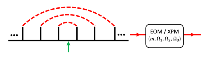
Figure 3: Phase modulation of a single QOFC. An OPO with a single pump frequency, whose half is denoted by the green arrow, creates TMS qumode pairs as indicated by the red dashed lines. Electro-optic phase modulation, or Kerr-medium cross phase modulation, is then done at index $m$ and frequencies $\Omega_{1,2,3}$.

A doubly resonant OPO is pumped at a single frequency $\omega_{p}$ such that frequency $\omega_{p}/2$ is set exactly halfway between 2 OPO mode frequencies (usually by a phaselock loop [9, 10]), as per the green arrow in Fig.3. This generates independent EPR qumode pairs in two-mode-squeezed (TMS) states [33, 43], a.k.a. the EPR QOFC. While entanglement scalability is already present in this case, it manifests itself only as the scaling of the number of copies of a bipartite EPR state, rather than as the scaling of the size of a multipartite state. Phase modulation by the EOM of the OPO QOFC will change that: by modulating at one, two or three frequencies, we can knit up 1D, 2D (square-grid), 3D (cubic) cluster states. We postulate that this extends to $n$-hypercubic cluster states, using $n$ modulation frequencies.

Note that, for every graph presented in this paper, we conducted a thorough analysis of the errors due to finite squeezing and imperfections due to nonlocal modulation couplings. This analysis will be detailed in Section III.

II.1 Generation of 1D cluster states

Following the steps in Sections I.2 & I.2.3, we derive the complex adjacency matrix $\bf Z$ of the created Gaussian state for $\Omega_{1}$=1, $r$=2.3, and for $m$=0, 0.1, 0.2, 0.5, and 1 rad. Figure 4 displays the real and imaginary parts of $\bf Z$, $\bf V$ and $\bf U$, after the appropriate LUs were applied; these LUs are Fourier transforms, i.e., rotations by $\pi/2$ in quadrature phase space $(Q,P)$, exerted on the lower-frequency-half qumodes, i.e., on all qumodes left of the green arrow in Fig.3).

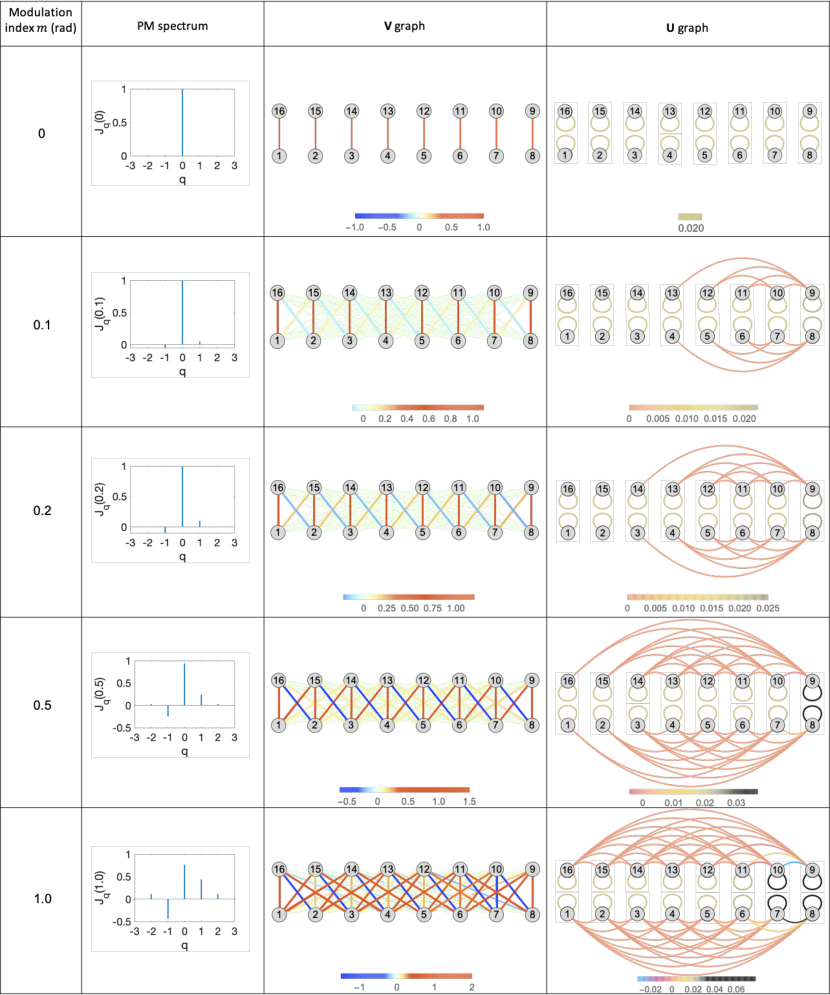
Figure 4: $\mathbf{V}$ and $\mathbf{U}$ graphs for the state generated by OPO-extrinsic PM at $\Omega_{1}$=1 and $r$=2.3, for different $m$. The pump frequency is equal to the sum of the frequencies of all vertical qumode pairs in the $\bf V$ and $\bf U$ graph columns. Note that the mode labeled “0” in the PM spectrum column is any of the QOFC qumodes in the $\bf V$ and $\bf U$ graph columns. All self loops that have the same color in each $\bf U$ graph have a value of 0.02, regardless of the value of $m$.

We can immediately see that phase modulation yields multipartite entanglement, which is a first essential result of this paper. We now examine the particular graphs that can be generated by this method, turning first to the effect of the modulation index parameter $m$. The initial case $m=0$ corresponds to EPR pairs from the OPO with no phase modulation. When the latter is turned on, additional edges are created, whose weights increase with $m$, as the EPR weights decrease. The classical FM spectra in the left column of Fig.4 give a good illustration of the effect on the quantum graph of the oscillations with $m$ of the Bessel-function amplitudes.

OPO-intrinsic versus OPO-extrinsic PM

In all cases presented in this paper, i.e., the 1D, 2D, and 3D graphs, we calculated both the extrinsic [Eq. (4)] and intrinsic [Eq. (5)] cases. We found that both methods give the same graphs, but that the intrinsic method has a lower level of error, as described in Section III. Because of the experimental simplicity of just placing an EOM after an OPO, we chose to present these extrinsic-OPO results in greater detail in Section II, also thereby placing an upper bound on the imperfections.

Back to Fig.4, the onset of next-nearest neighbor couplings in the quantum graph coïncides, unsurprisingly, with the growth of the first-order modulation sidebands, decrease of the carrier, and rise of the second harmonic sidebands. Such nonlocal graph edges are a known hindrance to one-way quantum computing [38, 39, 40]. However, we will show in Section III that this problem can be circumvented upon closer, rigorous inspection of the edges’ weights, which can always be found to be too small to be observable, when $m$ isn’t too large. Note also that this optimal $m$ will decrease as the squeezing parameter $r$ increases.

Remarkably, the imaginary part of the graph (rightmost column of Fig.4), given by the error matrix $\mathbf{U}$, complements the $\bf V$ graph, which clearly tends toward a complete bipartite graph with increasing $m$. In a sense, $\bf U$ leaves $\bf V$ globally invariant in terms of its bipartite structure, i.e., while $\bf V$ only connects qumode set $\{1,\dots,8\}$ to qumode set $\{9,\dots,16\}$ in Fig.4, $\bf U$ only connects qumodes within each of these two sets.

The same property that spurious edges can always be made small enough will appear in the $\mathbf{U}$ graph. In Section III, we will show that $\bf U$ is weak enough to validate this experimental technique.

Another crucial point that can be made immediately is that ${\rm Tr}[\mathbf{}\mathbf{U}]\to 0$ when $r\gg 1$, as required and illustrated in Fig.5, where ${\rm Tr}[\mathbf{}\mathbf{U}]$ is plotted and shown to adhere to the theoretical value obtained analytically for two-mode squeezed states [36].

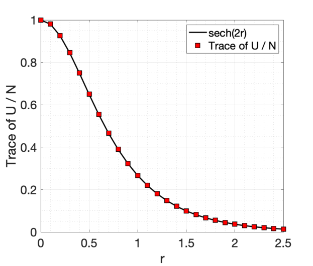
Figure 5: Plot of the average trace of $\bf U$ versus the squeezing parameter $r$, compared to the function $\text{sech}(2r)$. This $\mathbf{U}$ matrix is for the externally modulated QOFC at $\Omega_{1}$=1.

This point is important: it means that PM of two-mode-squeezed pairs doesn’t detract from the fact that the overall cluster state error is solely determined by the amount of initial squeezing. One should indeed, remember that $\bf U$, being symmetric positive semidefinite, must tend to zero as a whole when its trace tends to zero as per requirement (ii).

At this point, we anticipate the conclusions of the rigorous error analysis of Section III and ignore the weak edges in the whole complex graph to focus on the cluster states constructed by the dominant edges. We only have to limit the modulation index $m$ to low enough a value, keeping the PM couplings nearest-neighbor so as not to get nonlocal edges. The resulting graph is given by Fig.6(a).

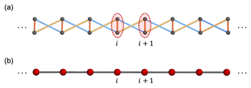
Figure 6: (a), $\bf V$ graph of Fig.4, revealing its typical structure for 1D cluster state. Two modes that are in the red dashed circle are the EPR-qumodes. (b), compact representation of the graph using EPR macronodes.

Swapping every other vertical pair of qumodes shows the graph to be a 1D “ladder” whose rungs are the initial EPR-pair qumodes. This dual graph structure connected by the initial EPR pairs will actually be a feature of the 2D and 3D graphs as well. In order to simplify the graph rendering in this case, we will bunch these EPR pairs into “EPR macronodes,” as in Fig.6(b). This ladder state spans the whole phasematching bandwidth of the OPO, which can reach 10 THz in our previous work [45]. With a typical mode spacing of 1GHz [9, 10], this yields on the order of $10^{4}$ entangled qumodes in this linear cluster state.

As is well known, the 1D graph isn’t enough to generate the universal gate set in one-way quantum computing, for which a 2D graph is required.

II.2 Generation of 2D cluster states

The experimental configuration of Fig.3 is surprisingly versatile: just adding modulation frequencies allows to increase the dimension of the graph lattice. Again, we send the reader to Section III for a detailed analysis of all graph imperfections and why they are negligible.

Driving the EOM with two modulation signals at frequencies $\Omega_{1,2}$ transforms Eq. (2) into

$$H_{PM2}=\hbar\left[{\frac{\alpha_{1}}{\tau}e^{-i\phi_{1}}\sum_{j=-\infty}^{\infty}a_{j}a_{j+\Omega_{1}}^{\dagger}+\frac{\alpha_{2}}{\tau}e^{-i\phi_{2}}\sum_{j=-\infty}^{\infty}a_{j}a_{j+\Omega_{2}}^{\dagger}}\right]+\text{H.c.}$$ (19)

Here we set $\phi_{1}=\phi_{2}=\pi/2$, $\alpha_{1}=\alpha_{2}$, and follow the same procedure as in the 1D case, which yields the square-grid cluster state of Fig.7.

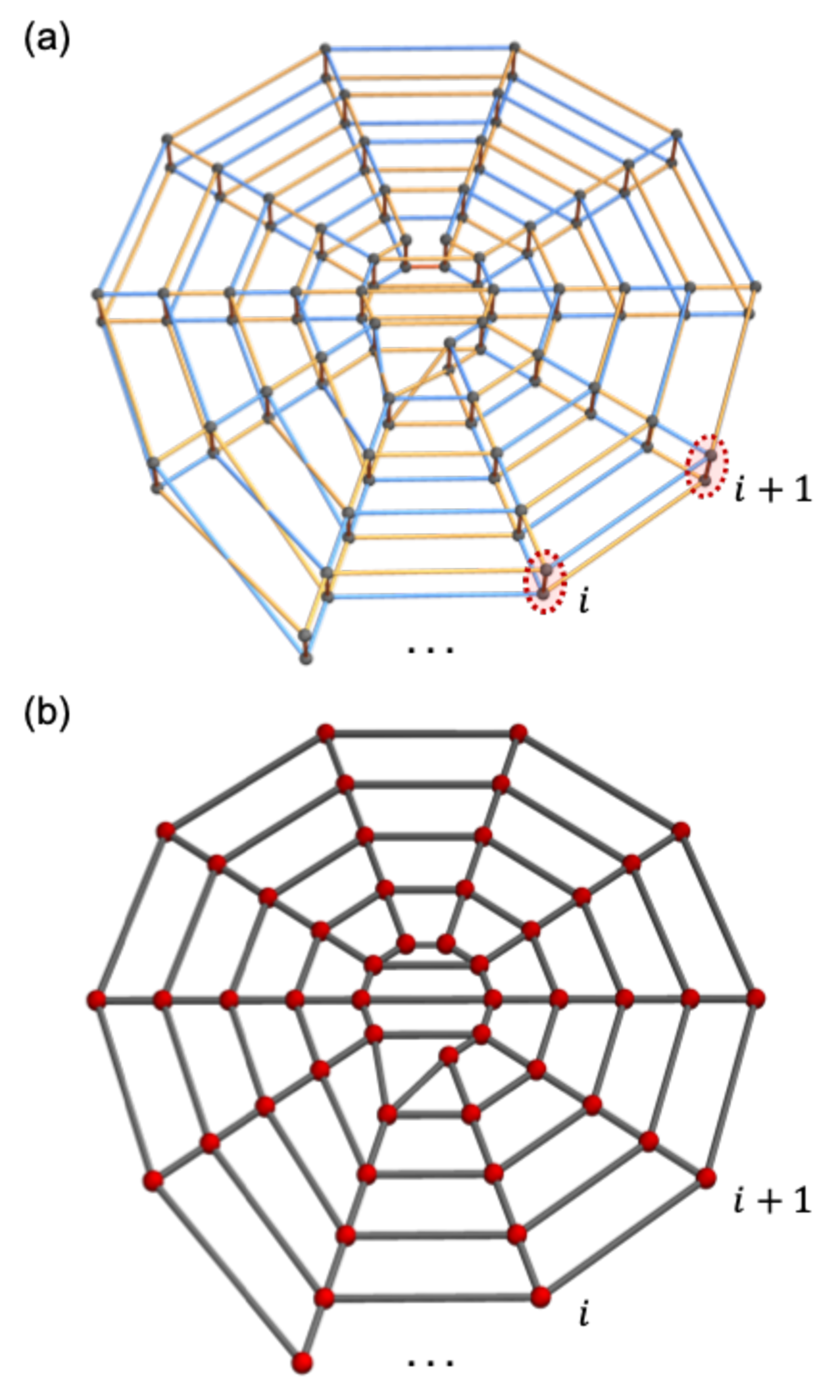
Figure 7: (a), square-grid cluster state created with $\Omega_{1}$=1, $\Omega_{2}$=10. Two modes circled by red dashed lines are EPR-qumodes, one of which is on the upper layer and the other one is on the bottom layer. (b), same graph, over EPR macronodes. The width of this square lattice is the number of “spokes” in the graph: $\Omega_{2}/\Omega_{1}=10$.

One can interpret this case in the following way: PM at frequency $\Omega_{1}$=1 creates next-neighbor coupling in the QOFC which forms a ladder graph; PM at frequency $\Omega_{2}$=10 then introduces additional coupling every 10 modes which is tantamount to spiraling the ladder into the two-layer square-grid cluster state of Fig.7(a). As in Fig.6(b), a more streamlined version of the graph can be obtained by considering EPR macronodes, Fig.7(b).

This is an important result because the square-grid cluster state is a resource for universal quantum computing.

As was mentioned earlier, the width of the square lattice, which is the number of ”spokes”, is simply the ratio $\Omega_{2}/\Omega_{1}$, the total number $N$ of qumodes being determined by the phasematching bandwidth of the OPO’s nonlinear medium. In the case of our previous experiments [9, 10], for which we estimated $N\sim 10^{4}$ [45], a 100 $\times$ 100 square cluster grid could therefore be created with PM at 1 and 100 GHz for a 1 GHz mode spacing. Note also that, in this case, the quasi-phasematching bandwidth can be further engineered to be larger.

II.3 Generation of 3D cluster states

At this point, we make the general claim that simply adding another modulation frequency adds another dimension to the EPR-macronode graph, extending this procedure to yield hypercubic cluster graphs. We illustrate this in the 3D case, which is relevant to quantum computing because the 3D architecture is a known base for implementing topological error encoding over cluster states [23].

With modulation frequencies $\{\Omega_{1},\Omega_{2},\Omega_{3}\}=\{1,8,80\}$, the quantum derivation yields the graph state pictured over EPR macronodes in Fig.8.

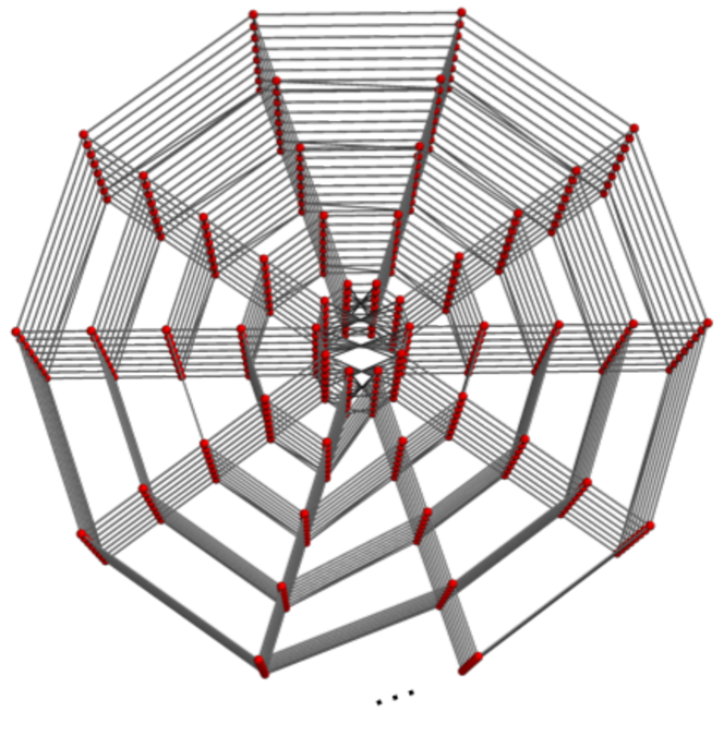
Figure 8: Cubic cluster state, over $N$=400 EPR macronodes, obtained from $\{\Omega_{1},\Omega_{2},\Omega_{3}\}=\{1,8,80\}$. Number of ”spokes”:10. Length: 8 macronodes. Spoke length: 5 macronodes.

The 6-edge valence of each graph vertex is clear in their vast majority. Note that, as always for cluster states, any local imperfections (graph center) in the graph can be removed by single-qumode measurements [6, 7, 35].

Finally, the ratio of PM frequencies determines the graph’s, here cylindrical, structure: the number of “spokes” is set by $\Omega_{3}/\Omega_{2}$ and the length of the cylinder is set by $\Omega_{2}/\Omega_{1}$. The radius of the spokes increases with the mode number $N$ as $N/\Omega_{3}$. In the example of Fig.8, a cubic cluster state is created over 400 macronodes in cylindrical shape with 10 ”spokes”, 5 set of macronodes in the radial direction, and a cylinder 8 macronodes long.

We now turn to the details of graph validation by scrutinizing the effects of the off-diagonal elements of $\bf U$.

III Graph error analysis

As we mentioned earlier, an arbitrary Gaussian state is a valid cluster state iff

(i), the error matrix U is diagonal [25] and,

(ii), it verifies ${\rm Tr}[\mathbf{U}]\to 0$ in the limit of infinite squeezing [36].

While requirement (ii) has been systematically fulfilled in all previous realizations of CV cluster states [47, 9, 10, 13, 14, 15], requirement (i) had not been considered until very recently [25], largely because all previous experimental realizations of cluster states had a diagonal $\bf U$. In this paper, $\bf U$ is not always diagonal, which can be seen as the price to pay for the considerable simplification of the experimental setup. We therefore evaluate the contribution of off-diagonal elements of $\bf U$ and determine the precise conditions under which they can be neglected.

Before we deal with error matrix $\bf U$, we first assume it fulfills both (i) and (ii) and focus on the effect of the weak, undesirable edges in $\bf V$ that can be seen in Fig.4 but not in Fig.6.

III.1 Effect of a spurious graph edge: bipartite case

We first take the simplest example of a canonical cluster state: in the unphysical limit of infinite squeezing, a single qumode 1 has, by definition, nullifier $P_{1}$. In the realistic case of finite squeezing, the exact nullifier of qumode 1 in a single-mode squeezed (SMS) state of squeezing parameter $r_{1}$ is

$$\mathcal{N}_{s1} =S_{1}(r_{1})\,a_{1}\,S_{1}^{\dagger}(r_{1})=P_{1}-ie^{-2r_{1}}\,Q_{1}.$$ (20)

These nullifiers are given by the complex $\bf Z$ graph, which always exists, but they are non-Hermitian, which makes the graph unsuited for quantum computing. A cluster state can be well defined as long as the imaginary part of $\bf Z$, $\bf U$, fulfills requirements (i,ii). Finite squeezing is not a problem so long as it reaches a fault tolerant value, which has been theoretically proven to be within experimental reach  [19].

Two phase-squeezed qumodes coupled by gate ${\rm C_{Z}}=\exp(i\varepsilon Q_{1}Q_{2})$ form a Gaussian cluster state of nullifiers

$$\mathcal{N}_{1} ={\rm C_{Z}}\,\mathcal{N}_{s1}\,{\rm C_{Z}}^{\dagger}=P_{1}-ie^{-2r_{1}}\,Q_{1}+\varepsilon\,Q_{2}$$ (21)

$$\mathcal{N}_{2} ={\rm C_{Z}}\,\mathcal{N}_{s2}\,{\rm C_{Z}}^{\dagger}=P_{2}-ie^{-2r_{2}}\,Q_{2}+\varepsilon\,Q_{1},$$ (22)

where $\bf U$ is diagonal and vanishes with increasing squeezing. We now ask the following question: if we wrongly assumed qumode 1 to be isolated when it is, in fact, linked to qumode 2 by a graph edge of small weight $\varepsilon$, how large could $\varepsilon$ be before its effects are detectable?

To answer this question, we must first relate it to the actual physical measurements we can make on qumode 1. Under the assumption that we have two single-mode phase-squeezed states, the lowest measurement noise should be obtained by measuring the phase quadrature operator $P_{1}$, typically by homodyne detection. In the case of a phase-squeezed qumode 1, observable $P_{1}$ has squeezed noise given by

$$(\Delta P_{1})^{2}={}_{1}\!\left\langle\,0\,\right|S_{1}(r_{1})^{\dagger}\,P_{1}^{2}\,S_{1}(r_{1})\left|\,0\,\right\rangle_{1}=\frac{1}{2}\,e^{-2r_{1}}.$$ (23)

We now assume $P_{1}$ when qumode 1 also has a $\rm C_{Z}$ graph edge of weight $\varepsilon$ with qumode 2 (squeezed by $r_{2}$), then we have

$$(\Delta P_{1})^{2} ={\,}_{12}\!\left\langle\,00\,\right|S_{2}^{\dagger}S_{1}^{\dagger}{\rm C_{Z}}^{{\dagger}}\,P_{1}^{2}\,{\rm C_{Z}}S_{1}S_{2}\left|\,00\,\right\rangle_{12}$$ (24)

$$={\,}_{12}\!\left\langle\,00\,\right|(P_{1}\,e^{-2r_{1}}-\varepsilon\,Q_{2}\,e^{2r_{2}})^{2}\left|\,00\,\right\rangle_{12}$$ (25)

$$=\frac{1}{2}\,e^{-2r_{1}}\left[1+\varepsilon^{2}\,e^{2(r_{1}+r_{2})}\right].$$ (26)

Comparing Eqs. (23) & (26), we deduce the condition for neglecting a graph edge of weight $\varepsilon$:

$$\varepsilon\ll\varepsilon_{\text{min}}=e^{-(r_{1}+r_{2})}$$ (27)

where $\varepsilon_{\text{min}}$ is the edge weight at which the quantum noise is raised by 3 dB on a single qumode quadrature measurement.

We now connect this reasoning to the formalism of Gaussian graphical calculus [36] and, in particular, Eq. (12). The procedure is the following: we define a “trimmed” version of the original graph Z=V+iU by zeroing all entries $\mathbf{V}_{jk}<\varepsilon_{\text{min}}$. In this case, it yields $\mathbf{V}^{\prime}=\mathbb{O}$ and a diagonal error matrix

$$\mathbf{U}^{\prime} =2\,\text{cov}[\mathbf{P}-\mathbf{V}^{\prime}\mathbf{Q}]$$ (28)

$$=2\,\text{cov}[\mathbf{P}]$$ (29)

$$=\begin{pmatrix}e^{-2r_{1}}\left[1+\varepsilon^{2}e^{2(r_{1}+r_{2})}\right]&0\\ 0&e^{-2r_{2}}\left[1+\varepsilon^{2}e^{2(r_{1}+r_{2})}\right]\end{pmatrix}$$ (30)

with the general condition for ${\rm Tr}[\mathbf{U}^{\prime}]\to 0$

$$\varepsilon\ll e^{-(r_{1}+r_{2})},$$ (31)

which is identical to Eq. (27).

III.2 Effect of spurious graph edges: multipartite case

As Eq. (15) makes clear, an off-diagonal element of $\bf U$ has the general physical meaning of a correlation between two cluster-state nullifiers. Such covariances must be zero in order for the cluster state to be adequate for one-way quantum computing. However, we can derive a good quantitative estimate of the level at which such covariances can be neglected, for a given squeezing level (${\rm Tr}[\mathbf{}\mathbf{U}]$) of the graph. This estimate is the error vector $\mathbf{\Gamma}$ defined by

$$\Gamma_{j}=\frac{1}{\mathbf{U}_{jj}}\sum_{k\neq j}|\mathbf{U}_{jk}|.$$ (32)

Assuming $\mathbf{U}_{jj}$ is of the order of a squeezing factor $e^{-2r_{j}}$ (see Fig.5), which ensures (ii), then (i) can be fulfilled if each and every qumode $j$ satisfies

$$\Gamma_{j}\ll 1.$$ (33)

This can even be relaxed a bit if one remember that local imperfections in cluster states can be measured out: if a majority of qumodes verify Eq. (33), then the few of them that don’t can be taken out of the graph by measuring $Q_{j}$ [7, 35].

The procedure of Eq. (28) can be straightforwardly applied to the multipartite case: after zeroing out weak edges in $\bf V$, we seek to diagonalize $\bf U$ by applying LUs, here Fourier transforms, i.e., rotations by $\pi/2$ in phase space, and inspect the final $\mathbf{U}^{\prime}$. If diagonalization wasn’t successful (it’s not always possible [25]), we evaluate $\mathbf{\Gamma}$ to assess the closeness of the state to a perfect cluster state.

Since we have noticed that $\bf U$ tends to be less and less diagonal as the dimensionality of the graph increases, we illustrate this procedure in the least favorable case of the cubic lattice produced by external PM. To obtain the graph of Fig.8 (as well as of Figs.6 & 7), all $\bf V$-edges weaker than a threshold value $\varepsilon_{\text{min}}$ were neglected. From this new $\mathbf{V}^{\prime}$, a new error matrix $\mathbf{U}^{\prime}$ was computed using Eq. (28).

Figure 9 displays the effect of such graph “trimming” on requirement (i), i.e., ${\rm Tr}[\mathbf{}\mathbf{U}]$ the cubic lattice cluster state, for different values of the squeezing parameter $r$.

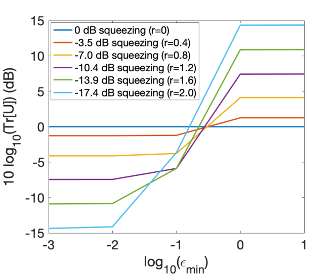
Figure 9: Effect of graph “trimming” (removing all graph edges smaller than $\varepsilon_{\text{min}}$), on the trace of $\mathbf{U}$, in the case of a cubic lattice produced by external FM. $\Omega_{1}=1$, $\Omega_{2}=8$, $\Omega_{3}=80$, $m=0.05$.

The important conclusion from this graph is that there always exist an $\varepsilon_{\text{min}}$ such that requirement (ii) is fulfilled. Hence, graph trimming can always be performed, no matter how large the squeezing is, which ensures one can perform graph trimming above the fault tolerance threshold.

We now turn to the equally critical requirement (i) for the cubic graph state of Fig.8. The components of error vector $\bf\Gamma$ of $\mathbf{U}^{\prime}$ were computed for all 1000 qumodes in the state and plotted in Fig.10,

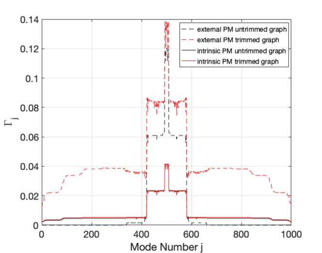
Figure 10: $\mathbf{\Gamma}$ plot for the cubic lattice, for PM either external or internal to the OPO. $\Omega_{1}=1$, $\Omega_{2}=8$, $\Omega_{3}=80$, $m=0.05$, $r=1.2$, $\varepsilon_{\text{min}}$=0.01.

which addresses both cases of cascaded EPR pair generation and PM, and integrated PM in the OPO. In the former case (black dashed lines), only a small portion of the graph (the center of Fig.8) has values of $\Gamma_{j}$ marginally larger than 0.1, and these can be measured out. Remarkably, the values of $\Gamma_{j}$ are close to zero for the vast majority of modes of the graph (0-400 and 600-1000), which corresponds to the bulk of the cubic lattice. Unsurprisingly, trimming the graph yields an increase of the error $\Gamma_{j}$ (red dashed lines) but, clearly, within manageable levels.

In the case of PM intrinsic to the OPO (solid lines), the cubic graph is clearly “cleaner” from the start as the values of $\mathbf{\Gamma}$ are much lower and trimming has much less of an effect.

IV Conclusion

We demonstrated that the “bare bone” resources constituted by a monochromatically pumped, below-threshold OPO along with phase modulation at multiples on the cavity spacing enable the generation of CV cluster states of arbitrary dimension, to arbitrarily low error level, compatible with the fault tolerance threshold predicted for CV quantum computing. The graph dimension is fully determined by the number and the ratio of phase modulation frequencies. For all squeezing levels, there exist modulation parameters that yield experimentally valid cluster states (see Supplemental Material). Of particular interest is the enhanced performance of phase modulation intrinsic to the OPO, as opposed to external to it. This experimental configuration is remarkably simple and compact and a marked simplification of all previous experimental realizations of large-scale cluster states, CV or otherwise. Note that these cluster states are deterministically and unconditionally generated, to the difference of other frequency-comb approaches that propose probabilistic linear-optics quantum computing [49] or employ postselected photonic qubits [50]. Note that the frequency bandwidth of the fastest modulator involved dictates the final size of the generated cluster state. Even though we have used, throughout this paper, the example of an EOM for the phase modulator, even faster options exist such as cross phase modulation in a Kerr medium, to which our analysis fully applies. Finally, the conceptual simplicity of this approach makes it well suited for implementations in integrated photonics.

Funding

This work was supported by NSF grants PHY-1820882, DMR-1839175, and EECS-1842641, and by BSF grant 2017743.

Disclosures

The authors declare no conflicts of interest.

Supplemental Documents

See Supplement 1 for supporting content.

References

- Pfister [2020] O. Pfister, Continuous-variable quantum computing in the quantum optical frequency comb, Journal of Physics B: Atomic, Molecular and Optical Physics 53, 012001 (2020).
- Pfister et al. [2004] O. Pfister, S. Feng, G. Jennings, R. Pooser, and D. Xie, Multipartite continuous-variable entanglement from concurrent nonlinearities, Phys. Rev. A 70, 020302 (2004).
- Menicucci et al. [2006] N. C. Menicucci, P. van Loock, M. Gu, C. Weedbrook, T. C. Ralph, and M. A. Nielsen, Universal quantum computation with continuous-variable cluster states, Phys. Rev. Lett. 97, 110501 (2006).
- Menicucci et al. [2008] N. C. Menicucci, S. T. Flammia, and O. Pfister, One-way quantum computing in the optical frequency comb, Phys. Rev. Lett. 101, 130501 (2008).
- Flammia et al. [2009] S. T. Flammia, N. C. Menicucci, and O. Pfister, The optical frequency comb as a one-way quantum computer, J. Phys. B, 42, 114009 (2009).
- Briegel and Raussendorf [2001] H. J. Briegel and R. Raussendorf, Persistent entanglement in arrays of interacting particles, Phys. Rev. Lett. 86, 910 (2001).
- Zhang and Braunstein [2006] J. Zhang and S. L. Braunstein, Continuous-variable Gaussian analog of cluster states, Phys. Rev. A 73, 032318 (2006).
- Raussendorf and Briegel [2001] R. Raussendorf and H. J. Briegel, A one-way quantum computer, Phys. Rev. Lett. 86, 5188 (2001).
- Pysher et al. [2011] M. Pysher, Y. Miwa, R. Shahrokhshahi, R. Bloomer, and O. Pfister, Parallel generation of quadripartite cluster entanglement in the optical frequency comb, Phys. Rev. Lett. 107, 030505 (2011).
- Chen et al. [2014] M. Chen, N. C. Menicucci, and O. Pfister, Experimental realization of multipartite entanglement of 60 modes of a quantum optical frequency comb, Phys. Rev. Lett. 112, 120505 (2014).
- Roslund et al. [2014] J. Roslund, R. Medeiros de Araújo, S. Jiang, C. Fabre, and N. Treps, Wavelength-multiplexed quantum networks with ultrafast frequency combs, Nat. Photon. 8, 109 (2014).
- Yokoyama et al. [2013] S. Yokoyama, R. Ukai, S. C. Armstrong, C. Sornphiphatphong, T. Kaji, S. Suzuki, J. Yoshikawa, H. Yonezawa, N. C. Menicucci, and A. Furusawa, Ultra-large-scale continuous-variable cluster states multiplexed in the time domain, Nat. Photon. 7, 982 (2013).
- Yoshikawa et al. [2016] J.-i. Yoshikawa, S. Yokoyama, T. Kaji, C. Sornphiphatphong, Y. Shiozawa, K. Makino, and A. Furusawa, Invited article: Generation of one-million-mode continuous-variable cluster state by unlimited time-domain multiplexing, APL Photonics 1, 060801 (2016).
- Asavanant et al. [2019] W. Asavanant, Y. Shiozawa, S. Yokoyama, B. Charoensombutamon, H. Emura, R. N. Alexander, S. Takeda, J.-i. Yoshikawa, N. C. Menicucci, H. Yonezawa, and A. Furusawa, Generation of time-domain-multiplexed two-dimensional cluster state, Science 366, 373 (2019), https://science.sciencemag.org/content/366/6463/373.full.pdf .
- Larsen et al. [2019] M. V. Larsen, X. Guo, C. R. Breum, J. S. Neergaard-Nielsen, and U. L. Andersen, Deterministic generation of a two-dimensional cluster state, Science 366, 369 (2019), https://science.sciencemag.org/content/366/6463/369.full.pdf .
- Armstrong et al. [2012] S. Armstrong, J.-F. Morizur, J. Janousek, B. Hage, N. Treps, P. K. Lam, and H.-A. Bachor, Programmable multimode quantum networks, Nat. Commun. 3:1026, 1 (2012).
- Pooser and Jing [2014] R. Pooser and J. Jing, Continuous-variable cluster-state generation over the optical spatial mode comb, Phys. Rev. A 90, 043841 (2014).
- Yang et al. [2020] R. Yang, J. Zhang, I. Klich, C. González-Arciniegas, and O. Pfister, Spatiotemporal graph states from a single optical parametric oscillator, Phys. Rev. A 101, 043832 (2020).
- Menicucci [2014] N. C. Menicucci, Fault-tolerant measurement-based quantum computing with continuous-variable cluster states, Phys. Rev. Lett. 112, 120504 (2014).
- Fukui et al. [2018] K. Fukui, A. Tomita, A. Okamoto, and K. Fujii, High-threshold fault-tolerant quantum computation with analog quantum error correction, Phys. Rev. X 8, 021054 (2018).
- Menicucci [2011] N. C. Menicucci, Temporal-mode continuous-variable cluster states using linear optics, Phys. Rev. A 83, 062314 (2011).
- Wang et al. [2014a] P. Wang, M. Chen, N. C. Menicucci, and O. Pfister, Weaving quantum optical frequency combs into hypercubic cluster states, Phys. Rev. A 90, 032325 (2014a).
- Raussendorf et al. [2006] R. Raussendorf, J. Harrington, and K. Goyal, A fault-tolerant one-way quantum computer, Ann. Phys. (NY) 321, 2242 (2006).
- Note [1] As we’ll show below, the phase modulator can be integrated in the OPO itself.
- González-Arciniegas et al. [2019] C. González-Arciniegas, P. Nussenzveig, M. Martinelli, and O. Pfister, Hidden multipartite entanglement in Gaussian cluster states, arXiv:1912.06463 [quant-ph] (2019), arXiv:1912.06463 [quant-ph] .
- Fürst et al. [2011] J. U. Fürst, D. V. Strekalov, D. Elser, A. Aiello, U. L. Andersen, C. Marquardt, and G. Leuchs, Quantum light from a whispering-gallery-mode disk resonator, Phys. Rev. Lett. 106, 113901 (2011).
- Dutt et al. [2015] A. Dutt, K. Luke, S. Manipatruni, A. L. Gaeta, P. Nussenzveig, and M. Lipson, On-chip optical squeezing, Phys. Rev. Applied 3, 044005 (2015).
- Lenzini et al. [2018] F. Lenzini, J. Janousek, O. Thearle, M. Villa, B. Haylock, S. Kasture, L. Cui, H.-P. Phan, D. V. Dao, H. Yonezawa, P. K. Lam, E. H. Huntington, and M. Lobino, Integrated photonic platform for quantum information with continuous variables, Sci. Adv. 4, 10.1126/sciadv.aat9331 (2018), https://advances.sciencemag.org/content/4/12/eaat9331.full.pdf .
- Mondain et al. [2019] F. Mondain, T. Lunghi, A. Zavatta, E. Gouzien, F. Doutre, M. D. Micheli, S. Tanzilli, and V. D’Auria, Chip-based squeezing at a telecom wavelength, Photon. Res. 7, A36 (2019).
- Vaidya et al. [2020] V. D. Vaidya, B. Morrison, L. G. Helt, R. Shahrokshahi, D. H. Mahler, M. J. Collins, K. Tan, J. Lavoie, A. Repingon, M. Menotti, N. Quesada, R. C. Pooser, A. E. Lita, T. Gerrits, S. W. Nam, and Z. Vernon, Broadband quadrature-squeezed vacuum and nonclassical photon number correlations from a nanophotonic device, Science Advances 6, 10.1126/sciadv.aba9186 (2020), https://advances.sciencemag.org/content/6/39/eaba9186.full.pdf .
- Capmany and Fernández-Pousa [2010] J. Capmany and C. R. Fernández-Pousa, Quantum model for electro-optical phase modulation, J. Opt. Soc. Am. B 27, A119 (2010).
- Note [2] Note that a full treatment of the OPO spectrum can be done using the input-output formalism [51] but it is not required here to capture the essential physics.
- Ou et al. [1992] Z. Y. Ou, S. F. Pereira, H. J. Kimble, and K. C. Peng, Realization of the Einstein-Podolsky-Rosen paradox for continuous variables, Phys. Rev. Lett. 68, 3663 (1992).
- Einstein et al. [1935] A. Einstein, B. Podolsky, and N. Rosen, Can quantum-mechanical description of physical reality be considered complete?, Phys. Rev. 47, 777 (1935).
- Gu et al. [2009] M. Gu, C. Weedbrook, N. C. Menicucci, T. C. Ralph, and P. van Loock, Quantum computing with continuous-variable clusters, Phys. Rev. A 79, 062318 (2009).
- Menicucci et al. [2011] N. C. Menicucci, S. T. Flammia, and P. van Loock, Graphical calculus for Gaussian pure states, Phys. Rev. A 83, 042335 (2011).
- Hein et al. [2004] M. Hein, J. Eisert, and H. J. Briegel, Multiparty entanglement in graph states, Phys. Rev. A 69, 062311 (2004).
- Bacon [2009] D. Bacon, Too entangled to quantum compute one-way, Physics 2, 38 (2009).
- Gross et al. [2009] D. Gross, S. T. Flammia, and J. Eisert, Most quantum states are too entangled to be useful as computational resources, Phys. Rev. Lett. 102, 190501 (2009).
- Bremner et al. [2009] M. J. Bremner, C. Mora, and A. Winter, Are random pure states useful for quantum computation?, Phys. Rev. Lett. 102, 190502 (2009).
- Yurke [1985] B. Yurke, Optical back-action-evading amplifiers, J. Opt. Soc. Am. B 2, 732 (1985).
- Note [3] Note that weighted graph states over qumodes are still stabilizer states, whereas they aren’t over qubits.
- Schori et al. [2002] C. Schori, J. L. Sörensen, and E. S. Polzik, Narrow-band frequency tunable light source of continuous quadrature entanglement, Phys. Rev. A 66, 033802 (2002).
- Note [4] Note that requirement (i) remains crucial as we cannot reach this infinite squeezing limit experimentally and, again, a fault tolerance threshold has been proven to exist in this case of finite squeezing [19].
- Wang et al. [2014b] P. Wang, W. Fan, and O. Pfister, Engineering large-scale entanglement in the quantum optical frequency comb: influence of the quasiphasematching bandwidth and of dispersion, arXiv:1403.6631 [physics.optics] (2014b).
- Note [5] Note that this is true even though the cluster state is a Gaussian state and that universal quantum computing requires non-Gaussian resources for exponential speedup and quantum error correction. This is strictly equivalent to the qubit case where cluster states stabilized by Pauli operators, globally invariant under Clifford operations (just like CV clusters are stabilized by Weyl-Heisenberg displacements, globally invariant under Gaussian operations), even though non-Clifford resources are required to achieve exponential speedup. In both cases, the necessary respective non-Gaussian and non-Clifford gates are realized by like measurements on the cluster state.
- Yukawa et al. [2008] M. Yukawa, R. Ukai, P. van Loock, and A. Furusawa, Experimental generation of four-mode continuous-variable cluster states, Phys. Rev. A 78, 012301 (2008).
- Note [6] Unsurprisingly, must decrease when increases. This will require lowering in turn so as to keep the spurious edges weak.
- Lukens and Lougovski [2017] J. M. Lukens and P. Lougovski, Frequency-encoded photonic qubits for scalable quantum information processing, Optica 4, 8 (2017).
- Kues et al. [2019] M. Kues, C. Reimer, J. M. Lukens, W. J. Munro, A. M. Weiner, D. J. Moss, and R. Morandotti, Quantum optical microcombs, Nature Photonics 13, 170 (2019).
- Gardiner and Zoller [2004] C. Gardiner and P. Zoller, Quantum Noise, A Handbook of Markovian and Non-Markovian Quantum Stochastic Methods with Applications to Quantum Optics, 3rd ed., Springer Series in Synergetics (Springer, 2004).