An Entropy-based Variable Feature Weighted Fuzzy k-Means Algorithm for High Dimensional Data

Abstract

This paper presents a new fuzzy k-means algorithm for the clustering of high dimensional data in various subspaces. Since, In the case of high dimensional data, some features might be irrelevant and relevant but may have different significance in the clustering. For a better clustering, it is crucial to incorporate the contribution of these features in the clustering process. To combine these features, in this paper, we have proposed a new fuzzy k-means clustering algorithm in which the objective function of the fuzzy k-means is modified using two different entropy term. The first entropy term helps to minimize the within-cluster dispersion and maximize the negative entropy to determine clusters to contribute to the association of data points. The second entropy term helps to control the weight of the features because different features have different contributing weights in the clustering process for obtaining the better partition of the data. The efficacy of the proposed method is presented in terms of various clustering measures on multiple datasets and compared with various state-of-the-art methods.

I Introduction

Clustering is a method that tries to organize unlabelled input data points into clusters or groups such that data points within a cluster have the most similarity than those belonging to different clusters, i.e., to maximize the intra-cluster similarity while minimizing the inter-cluster similarity. Based on belongingness, in the literature, clustering algorithms have been classified into various categories: hierarchical, density-based, grid-based, partition-based, and model-based clustering [1, 2, 3, 4]. Among them, the partition-based clustering is most widely studied. The most popular partition-based k-means algorithms reported in the literature are well known due to their performance in clustering large scale datasets, however these algorithms are susceptible to the initial cluster centers [5, 6, 7]. Ruspini [8] and Bezdek [9] have presented fuzzy variants of the k-means algorithm, where each data point can be a subset of multiple clusters with a different membership degree. However, the major problem with the k-means and fuzzy k-means algorithm remain the same, i.e., all features are assumed equally important during the clustering. Due to that, these algorithms are easily affected by the outliers.

To overcome the above limitations, feature weighted techniques had been studied by assigning different feature weight values based on the usefulness of the features in the identification of the clusters. In partition-based methods, k-means (KM)[10] and fuzzy c-means (FCM) [11] clustering algorithms have been more explored due to its simplicity and data handling characteristics. Feature weighted clustering algorithms, i.e, weighted k-means (WKM) [12], entropy weighted k-means (EWKM) [13], sparse k-means (SKM) [14], weighted fuzzy c-means (WFCM) [15], feature weighted FCM based on simultaneous clustering and attribute discrimination (SCAD) [16], and feature reduction FCM [17], have been studied in the past. The WKM is an extension of KM in which features are assigned equal weights to all clusters. The EWKM is the entropy weighted clustering method in which features are assigned distinct weights in the various clusters. The SKM uses the $L_{1}$ norm in the objective function, which helps for making the feature weights zero when the feature weights are smaller than a predefined threshold. To improve the learning performance of FCM, the WFCM is proposed in which the feature weights are learned through the gradient descent method. The SCAD is presented to improve the FCM performance by simultaneous clustering of the data with attribute discrimination.

The variable weighting of features in the clustering is an important research area in machine learning, which automatically determines the weight of each feature based on its significance in the clustering process [12, 13, 18]. For learning the number of cluster (k), the differences between clusters, based on the relevance of individual features in each cluster have been considered, which overcomes the problem of k-means and fuzzy k-means clustering algorithms in which all features are considered equally important during the clustering process. Specifically, for handling the sparse and high dimensional data, the contribution of each feature is essential, maybe some of the features are irrelevant, but they have different significance to the clustering process [19, 20].

For a better clustering, this paper present a novel entropy-based variable feature weighted fuzzy k-means algorithm for clustering the data by considering the different feature weights in each cluster. These features have various contributions to identify the data points in a cluster during the clustering process. The difference in the contribution of these features is formulated in terms of weight that can be expressed as the degree of certainty to the cluster. In the clustering, the decrease of the weight entropy in a cluster shows the increase of certainty of a subset of features with more substantial weights in the determination of the cluster. However, the membership entropy makes the clustering is insensitive to the initial cluster centers. In the proposed approach, we have simultaneously minimized inter-cluster dispersion, maximizes the negative data points-to-clusters membership entropy, and negative weight entropy to impel more number of features to contribute to the identification of a cluster.

The major contributions are briefly summarized as follows:

1. For handling the high dimensional, sparse and noisy data, the fuzzy k-means objective function is modified to increase the robustness using the fuzzy membership entropy with weight entropy in the objective function.

2. The fuzzy membership entropy helps in minimizing the within-cluster dispersion and maximize inter-cluster dispersion to identify the data points in a cluster.

3. The weighted feature entropy helps to simulate more dimensions to add different contributions for the identification of data points in a cluster.

The rest of the paper is organized as follows: Section II describes the proposed methodology. Experimentation and comparisons of the proposed method with various state-of-the-art methods are discussed in Section III. Finally, Section IV concludes the complete paper.

II Proposed Methodology

In this section, we present a novel entropy-based variable feature weighted fuzzy k-means clustering algorithm by considering the different contributions of each feature in each cluster. In the proposed approach, the weighted fuzzy k-means algorithm is combined with membership entropy and feature weighted entropy term simultaneously. As defined in (1) the first term measure the dissimilarity between the samples within clusters, the second term measures the membership entropy between samples and clusters during the clustering process, and the third term, i.e., the entropy of the feature weights, represents the degree of certainty to the features in the identification of a cluster.

Let us consider a data matrix $X=[X_{1},X_{2},\dots,X_{n}]\in R^{m\times n}$, $m$ and $n$ are the number of features and number of samples respectively. Here, $X_{i}=[x_{i1},x_{i2},\dots,x_{im}]^{\prime}\in R^{m}$ is the $i^{th}$ sample in the data matrix. To group the data matrix $X$ into $k$ number of clusters, the following objective function can be minimized

$$\begin{split}P(U,V,W)=\sum_{i=1}^{n}\sum_{j=1}^{k}\sum_{l=1}^{m}\mu_{ij}w_{jl}D_{ij}^{l}+\sum_{i=1}^{n}\lambda_{i}\sum_{j=1}^{k}\mu_{ij}\log\mu_{ij}\\ +\sum_{j=1}^{k}\gamma_{j}\sum_{l=1}^{m}w_{jl}\log w_{jl}\end{split}$$ (1)

subject to

$$\begin{split}\sum_{j=1}^{k}\mu_{ij}=1,\,\,0\leq\mu_{ij}\leq 1,\,\,1\leq i\leq n\\ and\\ \sum_{l=1}^{m}w_{jl}=1,\,\,0\leq w_{jl}\leq 1,\,\,1\leq j\leq k\end{split}$$ (2)

where, $D_{ij}^{l}=(x_{il}-v_{jl})^{2},$ is the dissimilarity measure between $i^{th}$ sample and $j^{th}$ cluster, $x_{il}$ is the value of $l^{th}$ feature of $i^{th}$ sample, $v_{jl}$ is the value of $l^{th}$ feature of $j^{th}$ cluster, $U=[u_{ij}]$ is the $n\times k$, fuzzy partition matrix, $u_{ij}$ is the membership degree value of the $j^{th}$ cluster of $i^{th}$ sample, $V=[v_{jl}]$ is the $k\times m$, matrix having the cluster centers, $W=[w_{jl}]$ is an $k\times m$, weight matrix, $w_{jl}$ is the weight value of $l^{th}$ feature to $j^{th}$ cluster, $\gamma_{i}$ and $\lambda_{j}$ are the input parameters used to control the fuzzy partition and feature weight, respectively.

II-A Optimization Procedure

The objective function, as given in (1), is a constrained nonlinear optimization problem whose solutions are unknown. The main aim is to minimize $P$ with respect to $U$, $V$, and $W$ using alternating optimization method. In the alternating optimization method, first we fix $U=\hat{U}$ and $W=\hat{W}$ and minimize $P$ with respect to $V$. Then we fix $U=\hat{U}$ and $V=\hat{V}$ and minimize $P$ with respect to $W$. Afterward, we fix $V=\hat{V}$ and $W=\hat{W}$ and minimize $P$ with respect to $U$.

First for the fixed $U$ and $W$ the objective function $P(U,V,W)$ is minimized with respect to $V$ as

$$\frac{\partial\hat{P}(U,V,W)}{\partial\hat{v}_{jl}}=-2\sum_{i=1}^{n}\mu_{ij}w_{jl}(x_{il}-v_{jl})=0$$ (3)

From (3) the cluster center can be obtained using

$$v_{jl}=\frac{w_{jl}\sum_{i=1}^{n}\mu_{ij}x_{il}}{w_{jl}\sum_{i=1}^{n}\mu_{ij}}$$ (4)

From the above equation two cases are arises.

Case 1: If $w_{jl}=0$, the $l^{th}$ feature is totally irrelevant respective to the $j^{th}$ cluster. Hence, for any value of $v_{jl}$, this feature will not contribute to the overall weighted distance computation. Therefore, in this case, any random value can be taken for $v_{jl}$.

Case 2: If $w_{jl}\neq 0$, the $l^{th}$ feature is relevant respective to the $j^{th}$ cluster, then the (4) is written as

$$v_{jl}=\frac{\sum_{i=1}^{n}\mu_{ij}x_{il}}{\sum_{i=1}^{n}\mu_{ij}}$$ (5)

Then for given $V=\hat{V}$, the constraint optimization problem in (1) is changed into unconstrained minimization problem using Lagrangian multiplier technique as follows:

$$\begin{split}\hat{P}(U,W,\alpha,\delta)=\sum_{i=1}^{n}\sum_{j=1}^{k}\sum_{l=1}^{m}\mu_{ij}w_{jl}D_{ij}^{l}+\sum_{i=1}^{n}\lambda_{i}\sum_{j=1}^{k}\mu_{ij}\log\mu_{ij}\\ +\sum_{j=1}^{k}\gamma_{j}\sum_{l=1}^{m}w_{jl}\log w_{jl}-\sum_{i=1}^{n}\alpha_{i}\left(\sum_{j=1}^{k}\mu_{ij}-1\right)\\ -\sum_{j=1}^{k}\delta_{j}\left(\sum_{l=1}^{m}w_{jl}-1\right)\end{split}$$ (6)

where, $\alpha=[\alpha_{1},\alpha_{2},\dots,\alpha_{n}]$ and $\delta=[\delta_{1},\delta_{2},\dots,\delta_{k}]$ are the vectors containing the Lagrangian multipliers. If $(\hat{U},\hat{W},\hat{\alpha},\hat{\delta})$ are the optimal values of $\hat{P}(U,W,\alpha,\delta)$, then the gradient with respect to these variable are vanishes.

$$\begin{split}\frac{\partial\hat{P}(U,W,\alpha,\delta)}{\partial\hat{\mu}_{ij}}=\sum_{l=1}^{m}w_{jl}D_{ij}^{l}+\lambda_{i}(1+\log\mu_{ij})-\alpha_{i}=0\\ 1\leq i\leq n,\,\,1\leq j\leq k,\end{split}$$ (7)

$$\begin{split}\frac{\partial\hat{P}(U,W,\alpha,\delta)}{\partial\hat{w}_{jl}}=\sum_{i=1}^{n}\mu_{ij}D_{ij}^{l}+\gamma_{j}(1+\log w_{jl})-\delta_{j}=0\\ 1\leq j\leq k,\,\,1\leq l\leq m,\end{split}$$ (8)

$$\frac{\partial\hat{P}(U,W,\alpha,\delta)}{\partial\hat{\alpha}_{i}}=\sum_{j=1}^{k}\mu_{ij}-1=0$$ (9)

and,

$$\frac{\partial\hat{P}(U,W,\alpha,\delta)}{\partial\hat{\delta}_{j}}=\sum_{l=1}^{m}w_{jl}-1=0$$ (10)

the (7) and (8) can be simplified as

$$\mu_{ij}=\exp\left(\frac{-\sum_{l=1}^{m}w_{jl}D_{ij}^{l}}{\lambda_{i}}\right)\exp\left(\frac{\alpha_{i}}{\lambda_{i}}\right)\exp(-1)$$ (11)

$$w_{jl}=\exp\left(\frac{-\sum_{i=1}^{n}\mu_{ij}D_{ij}^{l}}{\gamma_{j}}\right)\exp\left(\frac{\delta_{j}}{\gamma_{j}}\right)\exp(-1)$$ (12)

By substituting (11) in (9) and (12) in (10), we have

$$\begin{split}\sum_{j=1}^{k}\mu_{ij}=\sum_{j=1}^{k}\exp\left(\frac{-\sum_{l=1}^{m}w_{jl}D_{ij}^{l}}{\lambda_{i}}\right)\exp\left(\frac{\alpha_{i}}{\lambda_{i}}\right)\exp(-1)\\ =\exp\left(\frac{\alpha_{i}}{\lambda_{i}}\right)\exp(-1)\sum_{j=1}^{k}\exp\left(\frac{-\sum_{l=1}^{m}w_{jl}D_{ij}^{l}}{\lambda_{i}}\right)=1\\ \exp\left(\frac{\alpha_{i}}{\lambda_{i}}\right)\exp(-1)=\frac{1}{\sum_{j=1}^{k}\exp\left(\frac{-\sum_{l=1}^{m}w_{jl}D_{ij}^{l}}{\lambda_{i}}\right)}\end{split}$$ (13)

Similarly,

$$\begin{split}\sum_{l=1}^{m}w_{jl}=\sum_{l=1}^{m}\exp\left(\frac{-\sum_{i=1}^{n}\mu_{ij}D_{ij}^{l}}{\gamma_{j}}\right)\exp\left(\frac{\delta_{j}}{\gamma_{j}}\right)\exp(-1)\\ =\exp\left(\frac{\delta_{j}}{\gamma_{j}}\right)\exp(-1)\sum_{l=1}^{m}\exp\left(\frac{-\sum_{i=1}^{n}\mu_{ij}D_{ij}^{l}}{\gamma_{j}}\right)=1\\ \exp\left(\frac{\delta_{j}}{\gamma_{j}}\right)\exp(-1)=\frac{1}{\sum_{l=1}^{m}\exp\left(\frac{-\sum_{i=1}^{n}\mu_{ij}D_{ij}^{l}}{\gamma_{j}}\right)}\end{split}$$ (14)

By substituting (14) in (12) and (13) in (11), we obtain

$$w_{jl}=\frac{\exp\left(\frac{-\sum_{i=1}^{n}\mu_{ij}D_{ij}^{l}}{\gamma_{j}}\right)}{\sum_{l=1}^{m}\exp\left(\frac{-\sum_{i=1}^{n}\mu_{ij}D_{ij}^{l}}{\gamma_{j}}\right)}$$ (15)

$$\mu_{ij}=\frac{\exp\left(\frac{-\sum_{l=1}^{m}w_{jl}D_{ij}^{l}}{\lambda_{i}}\right)}{\sum_{j=1}^{k}\exp\left(\frac{-\sum_{l=1}^{m}w_{jl}D_{ij}^{l}}{\lambda_{i}}\right)}$$ (16)

As shown in (15) and (16) the feature weights within the cluster and membership degree of the data points are depend on each other. The dependency of both term on each other helps to find the better partition of the dataset which are reflected in the results and discussion section.

II-B Parameter Selection

The choice of parameters $\gamma_{j}$ and $\lambda_{i}$ in (15) and (16) are essential to the performance of the proposed approach since they reflect the importance of the second and third term relative to the first term in (1). The parameter $\lambda_{i}$ controls the clustering process in two ways: First, when $\lambda_{i}$ is large such that the first term in (1), i.e., within-cluster dispersion, is small in comparison to the second term, then the second term plays a crucial role to minimize (1). In the clustering process, it is trying to assign data points to more than one cluster to make the second term more negative. When the membership degrees $\mu_{ij}$ of a data point to all clusters are the same, the membership entropy value is large. Since the locations of points are fixed, to get the largest entropy, move the cluster centers to the same location. Second, when $\lambda_{i}$ is small, the first term is large, and it will play the role of minimizing the within-cluster dispersion. However, the control parameter $\gamma_{j}$ is used to control the feature weights, when $\gamma_{j}$ is positive, then the weight $w_{jl}$ as given in (15) is inversely proportional to $\sum_{i=1}^{n}\mu_{ij}D_{ij}^{l}$. The small of this term will make large $w_{jl}$, i.e., $l^{th}$ features in $j^{th}$ cluster are more important. If $\gamma_{j}$ in (15) is too large, the third term will dominate, and all features in $j^{th}$ cluster will be relevant and assigned equal weights of $\frac{1}{m}$. The parameters $\lambda_{i}$ and $\gamma_{j}$ in (15) and (16) are computed by (17) and (18) in iteration, t, as

$$\lambda_{i}=K_{1}\frac{\sum_{j=1}^{k}\sum_{l=1}^{m}\mu_{ij}^{t-1}w_{jl}^{t-1}(D_{ij}^{l})^{t-1}}{\sum_{j=1}^{k}\mu_{ij}^{t-1}\log\mu_{ij}^{t-1}}$$ (17)

$$\gamma_{j}=K_{2}\frac{\sum_{i=1}^{n}\sum_{l=1}^{m}\mu_{ij}^{t-1}w_{jl}^{t-1}(D_{ij}^{l})^{t-1}}{\sum_{l=1}^{m}w_{jl}^{t-1}\log w_{jl}^{t-1}}$$ (18)

The parameter $K_{1}$ and $K_{2}$ are a constant, and the superscript ($t-1$) represents the values in iteration ($t-1$). The presented approach is briefly described in Algorithm 1 as follows:

Algorithm 1 An Entropy based Variable Weighted Fuzzy k-Means Algorithm

1:Give the number of cluster $k,$ randomly initialize cluster center $V^{(0)},$ randomly initialize feature weight $W^{(0)},$ and initialize randomly control parameter $\lambda^{0}$ and $\gamma^{0}$

2:Repeat

3:Update the feature weight matrix $W$ using (15)

4:Update the fuzzy partition matrix $U$ using (16)

5:Update the cluster center matrix $V$ using (5)

6:Update parameters $\lambda_{i}$ and $\gamma_{j}$ using (17) and (18)

7:Until The objective function achieves its local minimum value or centers stabilize

Table I: dataset descriptions

Datasets	# of samples	# of features	# of cluster
Iris [21]	$150$	$4$	3
Ionosphere [21]	$351$	$34$	2
Ovarian cancer [22]	$253$	$15154$	2
Colon cancer [23]	$62$	$2000$	2
Ovarian cancer [24]	$216$	$4000$	2
Glioma [25]	$50$	$4434$	4
Lung cancer [25]	$203$	$3312$	$5$

Table II: performance measure in terms of AR, RI, and NMI (in %)

Datasets		KM [10]	EWKM [13]	AFKM [20]	FCM [11]	SCAD [16]	Proposed Approach
Iris [21]	AR	88.67	89.78	90.67	82.67	88.67	92.67
	RI	87.37	88.39	88.93	82.78	87.37	91.23
	NMI	74.19	77.80	72.44	65.22	74.19	78.99
Ionosphere [21]	AR	64.10	71.08	70.37	54.42	70.94	71.23
	RI	53.85	58.77	58.18	50.25	58.65	58.89
	NMI	00.00	13.35	12.64	02.53	12.99	13.49
Ovarian cancer [22]	AR	55.73	55.73	55.73	64.81	56.13	81.03
	RI	50.46	50.46	50.46	54.18	50.56	69.13
	NMI	00.71	00.71	07.00	07.44	00.95	27.11
Colon cancer [23]	AR	51.61	53.23	53.23	51.61	53.23	55.65
	RI	49.23	49.39	49.39	49.23	49.39	49.84
	NMI	02.27	04.59	01.27	01.27	04.59	05.33
Ovarian cancer [24]	AR	56.02	76.85	71.29	64.81	71.30	86.29
	RI	50.50	64.25	58.88	54.18	58.88	82.83
	NMI	00.00	32.24	18.19	07.44	18.76	46.95
Glioma [25]	AR	48.00	64.00	62.00	56.00	54.00	66.00
	RI	70.12	74.37	73.96	70.94	72.65	75.35
	NMI	44.45	51.86	49.41	46.74	49.61	47.86
Lung cancer [25]	AR	49.75	62.44	51.72	55.56	59.61	64.04
	RI	61.09	64.11	58.98	51.48	56.67	58.57
	NMI	45.75	49.16	42.50	27.33	19.99	26.86

Table III: performance measure in terms of PC, CE, XB and DI

Datasets			AFKM [10]	FCM [11]	SCAD[16]	Proposed Approach
	True cluster	Validity indices	Optimal cluster (values)	Optimal cluster (values)	Optimal cluster (values)	Optimal cluster (values)
Iris [21]	3	PC	3 (0.798)	3 (0.783)	3 (0.783)	3 (0.822)
		CE	3 (0.299)	3 (0.395)	3 (0.395)	3 (0.294)
		XB	3 (3.614)	3 (4.231)	3 (4.230)	3 (3.575)
		DI	3 (0.030)	3 (0.105)	3 (0.105)	3 (0.052)
Ionosphere [21]	2	PC	2 (0.500)	2 (0.651)	2 (0.651)	2 (0.729)
		CE	2 (0.693)	2 (0.521)	2 (0.521)	2 (0.394)
		XB	2 (2.061)	2 (3.156)	2 (3.157)	2 (3.176)
		DI	2 (0.081)	2 (0.071)	2 (0.071)	2 (0.082)
Ovarian cancer [22]	2	PC	2 (0.915)	2 (0.779)	2 (0.773)	2 (0.935)
		CE	2 (0.143)	2 (0.365)	2 (0.374)	2 (0.106)
		XB	2 (2.583)	2 (2.072)	2 (2.087)	2 (2.170)
		DI	2 (0.118)	2 (0.118)	2 (0.118)	2 (0.133)
Colon cancer [23]	2	PC	2 (0.500)	2 (0.568)	2 (0.568)	2 (0.733)
		CE	2 (0.693)	2 (0.622)	2 (0.622)	2 (0.394)
		XB	2 (0.982)	2 (0.997)	2 (0.997)	2 (1.114)
		DI	2 (0.311)	2 (0.326)	2 (0.326)	2 (0.271)
Ovarian cancer [24]	2	PC	2 (0.869)	2 (0.779)	2 (0.773)	2 (0.884)
		CE	2 (0.215)	2 (0.365)	2 (0.374)	2 (0.129)
		XB	2 (1.834)	2 (2.072)	2 (2.087)	2 (1.633)
		DI	2 (0.165)	2 (0.118)	2 (0.118)	2 (0.094)
Glioma [25]	4	PC	4 (0.465)	4 (0.252)	4 (0.263)	4 (0.637)
		CE	4 (0.926)	4 (1.382)	4 (1.360)	4 (0.664)
		XB	4 (0.607)	4 (0.406)	4 (0.405)	4 (0.910)
		DI	4 (0.434)	4 (0.474)	4 (0.397)	4 (0.412)
Lung cancer[25]	5	PC	5 (0.308)	5 (0.200)	5 (0.200)	5 (0.729)
		CE	5 (1.309)	5 (1.609)	5 (1.609)	5 (0.497)
		XB	5 (0.419)	5 (0.292)	5 (0.292)	5 (0.975)
		DI	5 (0.431)	5 (0.342)	5 (0.364)	5 (0.451)

III Results and Discussion

The proposed approach is validated on the various datasets as described in Table I and efficacy is presented in terms of various clustering performance measures such as accuracy rate (AR), rand index (RI) [26] and normalized mutual information (NMI) [27]. These performance measure are mathematically written as follows:

$$AR=\frac{1}{n}\sum_{j=1}^{k}n(k_{j})$$ (19)

$$RI=\frac{f_{1}+f_{2}}{f_{1}+f_{2}+f_{3}+f_{4}}$$ (20)

$$NMI=\frac{I(X:Y)}{[H(X)+H(Y)]/2}$$ (21)

where, $n(k_{j})$ denote the number of data points correctly obtained in cluster $j$, $n$ is the total number of data points. The large value of AR represents better clustering performance. The RI index is used to measure the similarity between the two clustering partitions. Let $k$ is the number of actual clusters, and $k^{*}$ is the number of clusters obtained through the various clustering methods. For a pair of points $(\text{x}_{i},\text{x}_{j})$, $f_{1}$ is the number of pairs of points that are the same in clusters $k$ and $k^{*}$, $f_{2}$ is the number of pairs of points that are same in cluster $k$ and different in cluster $k^{*}$, $f_{3}$ is the number of pairs of points that are different in cluster $k$, and same in cluster $k^{*}$, and $f_{4}$ is the number of pairs of points that are different in clusters $k$, and $k^{*}.$ In the clustering, NMI is used to measure the information of a term to contribute for making the correct classification decision, and its values always lie in between $0$ and $1$.

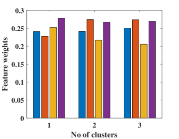
Figure 1: Feature weights for the IRIS dataset in all three clusters.

The above clustering performance measures are supervised i.e., a number of cluster k is known. However, it is generally unknown in clustering. Therefore, to find the effectiveness of proposed approach we have used different cluster validity indices, i.e., Partition Coefficient (PC) [28], Xie and Beni’s (XB) Index [29], Classification Entropy (CE) [30], and Dunn’s Index (DI) [31]. These validity indices are mathematically written as follows:

$$PC=\frac{1}{n}\sum_{j=1}^{k}\sum_{i=1}^{n}\mu_{ij}^{2}$$ (22)

$$CE=-\frac{1}{n}\sum_{j=1}^{k}\sum_{i=1}^{n}\mu_{ij}\log\mu_{ij}$$ (23)

$$XB=\frac{\sum_{j=1}^{k}\sum_{i=1}^{n}\mu_{ij}^{2}||x_{j}-v_{i}||^{2}}{n\min_{ij}||x_{j}-v_{i}||^{2}}$$ (24)

$$DI=\min_{i\in k}\Big{\{}\min{j\in k,i\neq j}\Big{\{}\frac{\min_{x\in k_{i},y\in k_{j}d(x,y)}}{\max_{i\in k}\{\max_{x,y\in k}d(x,y)\}}\Big{\}}$$ (25)

The range of PC lies in between $[1/k,1]$, if PC is closer to $1$ represents the best partition, whereas closer to $1/k$, the partition becomes fuzzier in the clustering. CE measures the fuzziness of the cluster partition similar to the PC, smaller the values of CE move towards the optimal cluster. In XB, the numerator represents the compactness of the fuzzy partition, and denominator denotes the strength between clusters, smaller the values of XB move towards the optimal cluster. DI measure the compactness in the well-separated clusters. The large value of DI represent better clustering results.

The proposed approach is validated on both small and high dimension datasets and compared with various state-of-the-art methods, i.e., KM, EWKM, AFKM, FCM, and SCAD. The KM algorithm gives equal importance to all features in the clustering and unable to provide the optimal clusters. This problem is overcome by the EWKM clustering, where different weight is assigned to the features in the clustering process. But the problem with this algorithm is in weight assignment because weight values depend on the initial cluster center. If the initial cluster center changed, the algorithm would lead to different clustering performance and unable converge. In the AFKM, an entropy term is added in the cost function to obtain the optimal cluster in the dataset, but the problem is that it treats all features equally in the clustering process. FCM assigns the soft partition of the data. Still, it gives equal importance to all features, however, in the SCAD they consider the different features weight in the different cluster, but they do not consider the entropy which controls the partition. In the proposed approach, the objective function is simultaneously optimized by taking weight entropy and fuzzy partition entropy. The weight entropy help to assign the relevant feature weight to the feature in the clustering whereas, fuzzy partition help to find the optimal number of the partition. The weight control and fuzzy partition control parameter in the case of EWKM and AFKM are heuristics, however, in the case of SCAD, weight control parameters are updated automatically in each iteration, but the fuzzy partition is not consistent. In the proposed approach, weight control and fuzzy partition control parameters are updated automatically in each iteration, and a better fuzzy partition is obtained due to relevant feature weight assignment during the clustering process.

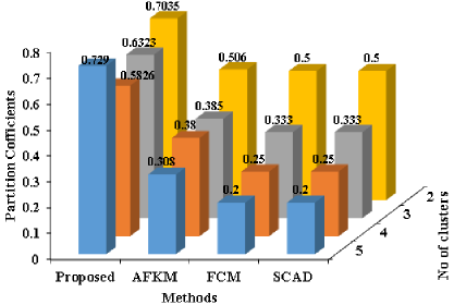
Figure 2: PC for the Lung dataset in varying the number of clusters.

As shown in Table II, the clustering performance in terms of AR, RI, and NMI of the proposed approach is much better for both high dimension and non-sparse datasets in comparison to state-of-the-art methods. The cluster validity index, i.e., PC, CE, XB, and DI, are also computed and compared with state-of-the-art methods, as given in Table III. The cluster validity measure shows that the proposed approach is able to provide the optimal clustering result with improved clustering performance. As shown in Table IV, the computational complexity of the proposed approach is little large in comparison to state-of-the-art methods due to the second and third term in the objective function. However, due to these terms, the clustering performance are improved.

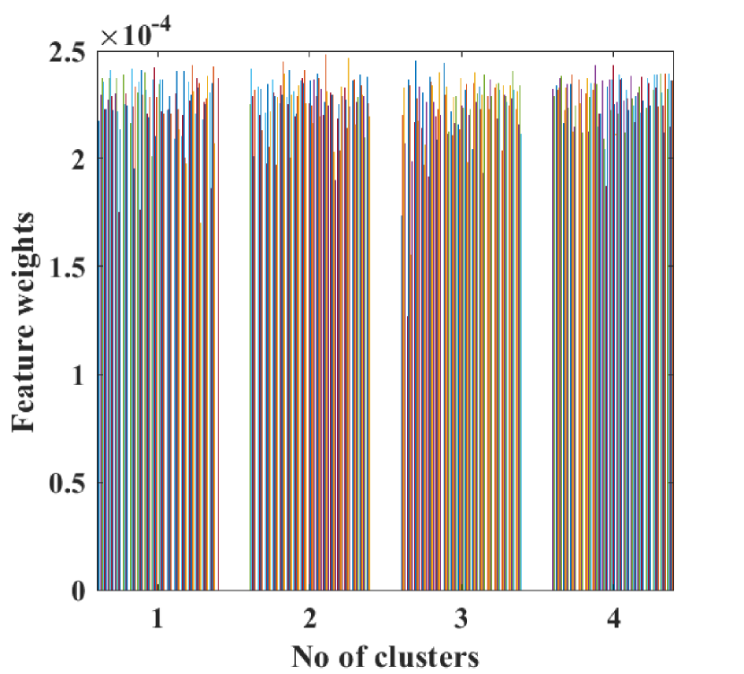
Figure 3: Feature weights for the GLIOMA dataset.

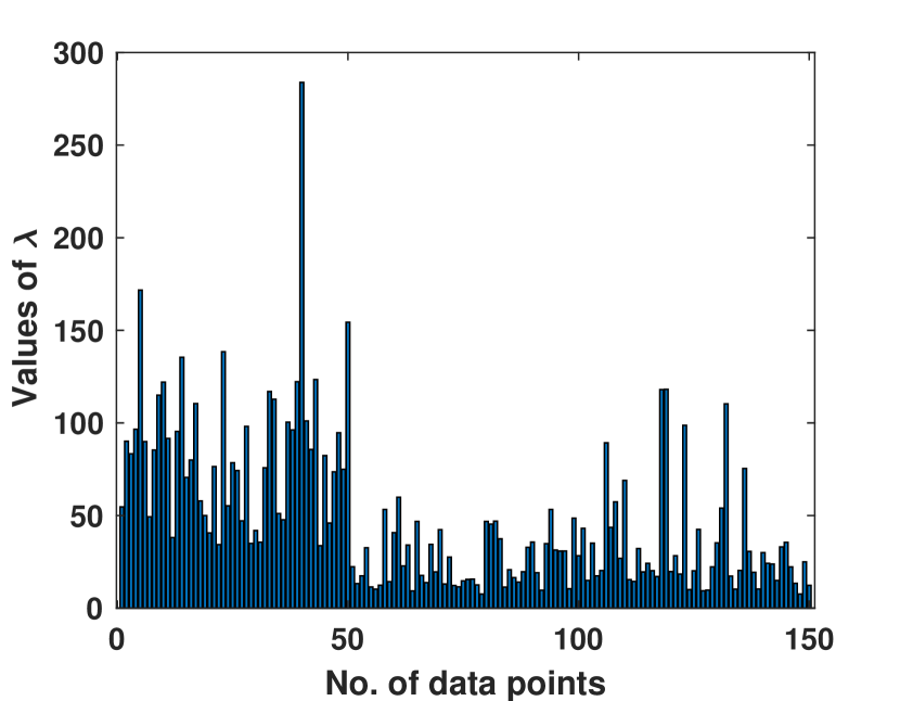
Figure 4: The values of $\lambda$ for the IRIS dataset

The contribution of weight in each cluster corresponding to the features is also plotted for the IRIS and GLIOMA dataset, as shown in Figures 1 and 4. As shown in Figures 1 and 4, the features have different weight contribution in each cluster, which generalize the approach. The fuzzy partition coefficients are shown in Figure 2 by varying the number of cluster which shows that proposed approach provide the better partition. The fuzzy partition control parameters are also plotted to show how parameters are changed from each iteration. The results in Tables II and III are computed by running all algorithms in ten trials independently, and average results are reported.

Table IV: computational complexity of the methods

Methodology	Computational Complexity
KM [10]	$O(nkm)$
EWKM [13]	$O(nkm^{2})$
AFKM [20]	$O(nk^{2}m)$
FCM [11]	$O(nk^{2}m)$
SCAD [16]	$O(nk^{2}m+nkm^{2})$
Proposed Approach	$O(nk^{2}m+nkm^{2})$

IV Conclusion

In this paper, an entropy-based variable feature weighted fuzzy k-means algorithm is presented for the clustering of high dimensional data with improved performance. In this approach, two different entropy terms are added in the objective function which helps in identifying the better clustering structure of the data. The major advantage of the presented method is that the clustering performance are consistent because it is insensitive to the initial cluster center due to the assignment of different feature weights to each cluster in the clustering process. The performance is compared with state-of-the-art methods in terms of different clustering measures, which shows that the proposed approach is a new clustering algorithm to partition the data with improved performance. In the future, correlation between the features can be considered to minimize the effect of redundant features, and the proposed method can be extended to categorical or mixed attributes.

References

- [1] J. C. Bezdek, Pattern recognition with fuzzy objective function algorithms. New York: Plenum, 1981.
- [2] G. Karypis, E.-H. S. Han, and V. Kumar, “Chameleon: Hierarchical clustering using dynamic modeling,” Computer, no. 8, pp. 68–75, 1999.
- [3] H.-P. Kriegel, P. Kröger, J. Sander, and A. Zimek, “Density-based clustering,” Wiley Interdisciplinary Reviews: Data Mining and Knowledge Discovery, vol. 1, no. 3, pp. 231–240, 2011.
- [4] C. Ordonez and E. Omiecinski, “FREM: fast and robust EM clustering for large data sets,” in Proceedings of the eleventh international conference on Information and knowledge Mgmt. ACM, 2002, pp. 590–599.
- [5] A. K. Jain and D. R. C., Algorithms for clustering data. Prentice Hall, 1988.
- [6] M. R. Anderberg, Clustering analysis for applications. Academic, 1988.
- [7] G. H. Ball and D. J. Hall, “A clustering technique for summarizing multivariate data,” Behavioral science, vol. 12, no. 2, pp. 153–155, 1967.
- [8] E. H. Ruspini, “A new approach to clustering,” Information and Control, vol. 15, no. 1, pp. 22–32, 1969.
- [9] J. C. Bezdek, “A convergence theorem for the fuzzy isodata clustering algorithms,” IEEE Transactions on Pattern Analysis & Machine Intelligence, no. 1, pp. 1–8, 1980.
- [10] J. MacQueen et al., “Some methods for classification and analysis of multivariate observations,” in Proceedings of the fifth Berkeley symposium on mathematical statistics and probability, vol. 1, no. 14. Oakland, CA, USA, 1967, pp. 281–297.
- [11] J. C. Bezdek, R. Ehrlich, and W. Full, “FCM: The fuzzy c-means clustering algorithm,” Computers & Geosciences, vol. 10, no. 2-3, pp. 191–203, 1984.
- [12] J. Z. Huang, M. K. Ng, H. Rong, and Z. Li, “Automated variable weighting in k-means type clustering,” IEEE Transactions on Pattern Analysis & Machine Intelligence, no. 5, pp. 657–668, 2005.
- [13] L. Jing, M. K. Ng, and J. Z. Huang, “An entropy weighting k-means algorithm for subspace clustering of high-dimensional sparse data,” IEEE Transactions on Knowledge & Data Engineering, no. 8, pp. 1026–1041, 2007.
- [14] D. M. Witten and R. Tibshirani, “A framework for feature selection in clustering,” Journal of the American Statistical Association, vol. 105, no. 490, pp. 713–726, 2010.
- [15] X. Wang, Y. Wang, and L. Wang, “Improving fuzzy c-means clustering based on feature-weight learning,” Pattern Recognition Letters, vol. 25, no. 10, pp. 1123–1132, 2004.
- [16] H. Frigui and O. Nasraoui, “Unsupervised learning of prototypes and attribute weights,” Pattern Recognition, vol. 37, no. 3, pp. 567–581, 2004.
- [17] S. Yang, Miin and Y. Nataliani, “A feature-reduction fuzzy clustering algorithm based on feature-weighted entropy,” IEEE Transactions on Fuzzy Systems, vol. 26, no. 2, pp. 817–835, 2017.
- [18] D. S. Modha and W. S. Spangler, “Feature weighting in k-means clustering,” Machine Learning, vol. 52, no. 3, pp. 217–237, 2003.
- [19] X. Chen, et al., “TW-k-means: Automated two-level variable weighting clustering algorithm for multiview data,” IEEE Transactions on Knowledge & Data Engineering, vol. 25, no. 4, pp. 932–944, 2011.
- [20] M. J. Li et al., “Agglomerative fuzzy k-means clustering algorithm with selection of number of clusters,” IEEE Transactions on Knowledge & Data Engineering, vol. 20, no. 11, pp. 1519–1534, 2008.
- [21] D. Dua and C. Graff, “UCI machine learning repository,” 2017. [Online]. Available: http://archive.ics.uci.edu/ml
- [22] http://cilab.ujn.edu.cn/datasets.htm, [Online; accessed 01-Nov-2019].
- [23] U. Alon, et al., “Broad patterns of gene expression revealed by clustering analysis of tumor and normal colon tissues probed by oligonucleotide arrays,” Proceedings of the National Academy of Sciences, vol. 96, no. 12, pp. 6745–6750, 1999.
- [24] https://in.mathworks.com/help/stats/sample-data-sets.html, [Online; accessed 01-Nov-2019].
- [25] http://featureselection.asu.edu/datasets.php, [Online; accessed 01-Nov-2019].
- [26] W. M. Rand, “Objective criteria for the evaluation of clustering methods,” Journal of the American Statistical Association, vol. 66, no. 336, pp. 846–850, 1971.
- [27] X. He, D. Cai, and P. Niyogi, “Laplacian score for feature selection,” in Advances in Neural Information Processing Systems, 2006, pp. 507–514.
- [28] J. C. Bezdek, “Numerical taxonomy with fuzzy sets,” Journal of Mathematical Biology, vol. 1, no. 1, pp. 57–71, 1974.
- [29] X. L. Xie and G. Beni, “A validity measure for fuzzy clustering,” IEEE Transactions on Pattern Analysis & Machine Intelligence, no. 8, pp. 841–847, 1991.
- [30] J. C. Bezdek, “Cluster validity with fuzzy sets,” 1973.
- [31] J. C. Dunn, “Well-separated clusters and optimal fuzzy partitions,” Journal of Cybernetics, vol. 4, no. 1, pp. 95–104, 1974.