Quadruply Stochastic Gradient Method for Large Scale Nonlinear Semi-Supervised Ordinal Regression AUC Optimization

Abstract

Semi-supervised ordinal regression (S²OR) problems are ubiquitous in real-world applications, where only a few ordered instances are labeled and massive instances remain unlabeled. Recent researches have shown that directly optimizing concordance index or AUC can impose a better ranking on the data than optimizing the traditional error rate in ordinal regression (OR) problems. In this paper, we propose an unbiased objective function for S²OR AUC optimization based on ordinal binary decomposition approach. Besides, to handle the large-scale kernelized learning problems, we propose a scalable algorithm called QS³ORAO using the doubly stochastic gradients (DSG) framework for functional optimization. Theoretically, we prove that our method can converge to the optimal solution at the rate of $O(1/t)$, where $t$ is the number of iterations for stochastic data sampling. Extensive experimental results on various benchmark and real-world datasets also demonstrate that our method is efficient and effective while retaining similar generalization performance.

Introduction

Supervised ordinal regression (OR) problems have made great process in the past few decades, such as (?; ?; ?; ?; ?). However, in various practical fields, such as facial beauty assessment (?), credit rating (?), social sciences (?) or more, collecting a large amount of ordinal labeled instances is time-consuming, while unlabeled data are available in abundance. Often, the finite ordinal data are insufficient to learn a good ordinal regression model. To improve the performance of the classifiers, one needs to incorporate unlabeled instances into the training process. So far, semi-supervised ordinal regression (S²OR) problems have attracted great attention in machine learning communities, such as (?; ?).

To evaluate the performance of an OR model, many metrics could be used, e.g., the mean absolute error, the mean squared error. However, Waegeman, De Baets and Boullart, (?) have shown that OR models which minimize these errors do not necessarily impose a good ranking on the data. To handle this problem, many researchers start to use AUC or concordance index in solving OR problems since AUC is defined on an ordinal scale, such as (?; ?; ?; ?). We summarized several representative OR algorithms in Table 1.

However, existing AUC optimization methods focus on supervised OR problems, and none of them can be applied to semi-supervised learning problems. The main challenge is how to incorporate unlabeled instances into the AUC optimization process. For the semi-supervised learning research field in general, many existing methods, such as (?; ?), have leveraged the cluster assumptions, which states that similar instances tend to share the same label, to solve this problem. However, the clustering assumption is rather restrictive and may mislead a model towards a biased solution. Nevertheless, recent works (?; ?) have shown that the clustering assumption is actually unnecessary at least for binary classification problems. In the same vein, we propose an objective function of S²OR AUC optimization based on ordinal binary decomposition without using the clustering assumption. Specifically, for a $k$ classes OR problem, we use $k-1$ hyperlanes to decompose the orginal problem into $k-1$ binary semi-supervised AUC optimization problems, where the AUC risk can be viewed as a linear combination of AUC risk between labeled instances and AUC risk between labeled and unlabeled instances. Then, the overall AUC risk in S²OR is equivalent to the mean of AUC for $k-1$ subproblems.

Table 1: Several representative OR algorithms. ($D$ denotes the number of random features, $k$ denotes the number of classes, $n$ denotes the number of training samples, and $t$ denotes number of iterations.)

Learning setting	Algorithm	Reference	AUC	Computational complexity	Space complexity
Supervised	ALOR	Fathony et al, (?)	No	$O(n^{3})$	$O(n^{2})$
	SVOREX	Chu et al, (?)	No	$O(n^{3})$	$O(n^{2})$
	VUS	Waegeman et al, (?)	Yes	$O(n^{3})$	$O(n^{2})$
	MultiRank	Uematsu and Lee, (?)	Yes	$O(n^{3})$	$O(n^{2})$
Semi-supervised	TOR	Seah et al, (?)	No	$O(n^{3})$	$O(n^{2})$
	SSORERM	(?)	No	$O(n^{3})$	$O(n^{2})$
	SSGPOR	Srijith et al, (?)	No	$>O(n^{3})$	$O(n^{2})$
	ManifoldOR	Liu et al, (?)	No	$O(n^{3})$	$O(n^{2})$
	QS3ORAO	Ours	Yes	$O(Dt^{2})$	$O(Dn)$

Nonlinear data structures widely exist in many real-world problems, and kernel method is a typical way to solve such problems. However, kernel-based methods are hardly scalable. Specifically, the kernel matrix needs $O(n^{2}d)$ operations to be calculated and $O(n^{2})$ to be stored, where $n$ denotes the number of training data and $d$ denotes the dimensionality of the data. Besides, the bottlenecks of the computational complexities become more severe in solving pairwise learning problems such as AUC optimization. In addition, as required by AUC computation, the OR learning problem needs to be decomposed into several binary classification sub-problems, which further increases the problem size and computational complexity. Thus, the new challenge is how to scale up kernel-based S²OR AUC optimization.

Scaling up kernel method has attracted greate attend in machining (?; ?; ?; ?; ?). Recently, Dai et al, (?) proposed doubly stochastic gradient (DSG) method to scale up kernel-based algorithms. Specifically, in each iteration, DSG randomly samples a data instance and its random features to compute the doubly stochastic functional gradient, and then the model function can be updated by using this gradient. However, the original DSG cannot be applied to solve the kernel-based S²OR AUC optimization. On the one hand, optimizing AUC is a pairwise problem which is much more complicated than the pointwise problem considered in standard DSG framework. On the other hand, S²OR optimization problems need to handle two different types of data, i.e., unlabeled dataset and the datasets of class $i$, while standard DSG focuses on minimizing the empirical risk on a single dataset with all data instances labeled.

To address these challenging problems, inspride by (?; ?), we introduce multiple sources of randomness. Specifically, we randomly sample a positive instance, a negative instance, an unlabeled instance, and their random features in each subproblem to calculate the approximated stochastic gradients of our objective function in each iteration. Then the ranking function can be iteratively updated. Since we randomly sample instances from four data sources in each subproblem, we denote our method as quadruply stochastic gradient S²OR AUC optimization method (QS³ORAO). Theoretically, we prove that our proposed QS³ORAO can converge to the optimal solution at the rate of $O(1/t)$. Extensive experimental results on benchmark datasets and real-world datasets also demonstrate that our method is efficient and effective while retaining similar generalization performance.

Contributions. The main contributions of this paper are summarized as follows.

1. We propose an objective function for solving S²OR AUC optimization problems in an unbiased manner. To the best of our knowledge, this is the first objective formulation incorporating the unlabeled data into the AUC optimization process in OR problems.

2. To optimize the objective function under the kernel learning setting, we propose an efficient and scalable S²OR AUC optimization algorithm, QS³ORAO, based on DSG framework.

3. We provide the convergence analysis of QS³ORAO, which indicates that an ideal $O(1/t)$ convergence rate is possible under certain mild assumptions.

Related Works

Semi-Supervised Ordinal Regression

In real-world applications, labeled instances are often costly to calibrate or difficult to obtain. This has led to a lot of efforts to study how to make full use of unlabeled data to improve the accuracy of classification, such as (?; ?; ?). Many existing methods incorporate unlabeled instances into learning propose by using various restrictive assumptions. For example, Seah, Tsang and Ong, (?) proposed TOR based on cluster assumption, where the instances share the same label if there are close to each other. Liu et al, (?) proposed a semi-supervised OR method, ManifoldOR, based on the assumption that the input data are distributed into a lower-dimensional manifold (?). Besides, Srijith et al, (?) proposed SSGPOR based on the low density separation assumption (?). We summarized these semi-supervised OR algorithms in Table 1. Note, in our semi-supervised OR AUC method, we do not need these restrictive assumptions.

Kernel Approximation

Kernel approximation is a common method to scale up kernel-based algorithms, which can be decomposed into two categories. One is data-dependent methods, such as greedy basis selection techniques (?), incomplete Cholesky decomposition (?), Nyström method (?). In order to achieve a low generalization performance, these methods usually need a large amount of training instances to compute a low-rank approximation of the kernel matrix, which may have high memory requriement. Another one is data-independent methods, which directly approximates the kernel function unbiasedly with some basis functions, such as random Fourier feature (RFF) (?). However, RFF method needs to save large amounts of random features. Instead of saving all the random features, Dai et al, (?) proposed DSG algorithm to use pseudo-random number generators to generate the random features on-the-fly, which has been widely used (?; ?; ?). Our method can be viewed as an extension of (?). However, OR is much more complicated than binary classification, since OR involves $k$ classes with ordering constraint, while (?) only studies binary classification. How the $k$ ordered classes could be learnt under the DSG framework is a novel and challenging problem. Theoretically, whether and to what extent the convergence property remains true is also a non-trivial problem.

Preliminaries

In this section, we first give a brief review of the AUC optimization framework in supervised ordinal regression settings, and then we propose our objective function in S²OR AUC optimization problems. Finally, we give a brief review of random Fourier features.

Supervised Ordinal Regression AUC Optimization

Let $x\in\mathbb{R}^{d}$ be a $d$-dimensional data instance and $y=\{1,\cdots,k\}$ be the label of each instance. Let $p(x,y)$ be the underlying joint distribution density of $\{x,y\}$. In supervised OR problems, the labeled datasets of each class can be viewed as drawn from the conditional distributional density $p(x|y)$ as follows,

$$\mathcal{D}_{j}=\{x_{i}^{j}\}_{i=1}^{n_{j}}\sim p(x|y=j),\;j=1,\cdots,k.$$

Generally speaking, the vast majority of existing ordinal regression models can be represented as ,

$$h(x)=\left\{\begin{matrix}1,&\mathrm{if}&f(x)<b_{1}\\ j,&\mathrm{if}&b_{j-1}<f(x)<b_{j},j=2,\cdots,k-1\\ k,&\mathrm{if}&f(x)>b_{k-1}\end{matrix}\right.,$$

where $b_{1}<\cdots<b_{k-1}$ denote the thresholds and $f:\mathbb{R}^{d}\mapsto\mathbb{R}$ is commonly referred as a ranking function (?). The model $h$ means that we need to consider $k-1$ parallel hyperplanes, $f(x)-b_{j}$, which decompose the ordinal target variables into $k-1$ binary classification subproblems. Therefore, the problem of calculating the AUC in OR problems can be transformed to that of calculating AUC in $k-1$ binary subproblems.

In binary classification, AUC means the probability that a randomly sampled positive instance receive a higher ranking than a randomly drawn negative instance. Thus, to calculate AUC in $j$-th subproblem, we need to define which part is positive. Fortunately, in OR problems, instances can naturally be ranked by their ordinal labels. Therefore, for the $j$-th binary classification hyperplane, the first consecutive $j$ categories, $1,\cdots,j$, can be regarded as negative, and the rest of the classes, ${j+1},\cdots,k$, can be regarded as positive. Then we obtain two new datasets as follows,

$$\mathcal{D}_{n}^{j}=\mathcal{D}_{1}\cup\cdots\cup\mathcal{D}_{j}\sim p^{j}_{-}=\dfrac{\sum_{i=1}^{j}\theta_{i}p(x|y=i)}{\sum_{i=1}^{j}\theta_{i}},$$

$$\mathcal{D}_{p}^{j}=\mathcal{D}_{j+1}\cup\cdots\cup\mathcal{D}_{k}\sim p^{j}_{+}=\dfrac{\sum_{i=j+1}^{k}\theta_{i}p(x|y=i)}{\sum_{i=j+1}^{k}\theta_{i}},$$

where $\theta_{i}$ denotes class prior of each class. Then AUC in each binary subproblem can be calculated by

$$\mathrm{AUC}=1-\mathbb{E}_{x_{p}^{j}\sim p^{j}_{+}}\left[\mathbb{E}_{x_{n}^{j}\sim p^{j}_{-}}\left[l_{01}\left(f(x_{p}^{j}),f(x_{n}^{j})\right)\right]\right],$$

where $l_{01}(u,v)=\dfrac{1}{2}\left(1-\mathrm{sign}(u-v)\right)$ and $\mathbb{E}_{x\sim p(\cdot)}$ denotes the expectation over distribution $p(\cdot)$. The zero-one loss can be replaced by squared pairwise loss function $l_{s}(u,v)=(1-u+v)^{2}$ (?; ?). While in real-world problems, the distribution is unknown and one usually uses the empirical mean to replace the expectation. Thus, the second term can be rewritten as

$$R^{j}_{\mathrm{PN}} =\mathbb{E}_{x_{p}^{j}\in\mathcal{D}_{p}^{j}}\left[\mathbb{E}_{x_{n}^{j}\in\mathcal{D}_{n}^{j}}\left[l_{01}\left(f(x_{p}^{j}),f(x_{n}^{j})\right)\right]\right],$$ (1)

where $\mathbb{E}_{x\in\mathcal{D}}$ denotes the empirical mean on the dataset $\mathcal{D}$. Equation (1) can be viewed as AUC risk between positive and negative instances. Obviously, maximizing AUC is equivalent to minimizing AUC risk $R_{\mathrm{PN}}$.

According to (?), the goal of AUC optimization in OR problems is to train a ranking function $f$ which can minimize the overall AUC risk of $k-1$ subproblems,

$$R_{\alpha}=\dfrac{1}{k-1}\sum_{j=1}^{k-1}R^{j}_{\mathrm{PN}}.$$ (2)

Semi-Supervised Ordinal Regression AUC Optimization

In semi-supervised OR problems, the unlabeled data can be viewed as drawn from the marginal distribution $p(x)$ as follows,

$$\mathcal{D}_{u}=\{x_{i}^{u}\}_{i=1}^{n_{u}}\sim p(x),$$ (3)

where $p(x)=\sum_{j=1}^{k}\theta_{j}p(x|y=j)$. For the $j$-th subproblem, the unlabeled data can be viewed as drawn from distribution $p^{j}(x)=\pi^{j}p^{j}_{+}+(1-\pi^{j})p^{j}_{-}$, where $\pi^{j}=\sum_{i=j+1}^{k}\theta_{i}$.

The key idea to incorporate the unlabeled instances into the binary AUC optimization process is to treat the unlabeled instances as negative and then compare them with positive instances; treat them as positive and compare them with negative data (?). Thus, the AUC risk $R^{j}_{\mathrm{PU}}$ between positive and unlabeled instances and the AUC risk $R^{j}_{\mathrm{NU}}$ between unlabeled and negative instances can be defined as follow,

$$R_{\mathrm{PU}}^{j} =\mathbb{E}_{x_{p}^{j}\in\mathcal{D}_{p}^{j}}\left[\mathbb{E}_{x_{u}^{j}\in\mathcal{D}_{u}}\left[l_{01}\left(f(x_{p}^{j}),f(x_{u}^{j})\right)\right]\right],$$ (4)

$$R_{\mathrm{NU}}^{j} =\mathbb{E}_{x_{u}^{j}\in\mathcal{D}_{u}}\left[\mathbb{E}_{x_{n}^{j}\in\mathcal{D}_{n}^{j}}\left[l_{01}\left(f(x_{u}^{j}),f(x_{n}^{j})\right)\right]\right],$$ (5)

Xie and Li, (?) have shown that $R^{j}_{\mathrm{PU}}$ and $R^{j}_{\mathrm{NU}}$ are equivalent to $R^{j}_{\mathrm{PN}}$ with a linear transformation as follows,

$$R^{j}_{\mathrm{PN}}=R^{j}_{\mathrm{PU}}+R^{j}_{\mathrm{NU}}-\dfrac{1}{2}.$$ (6)

Thus, the AUC risk $R^{j}_{\mathrm{PNU}}$ for the $j$-th binary semi-supervised problem is

$$R^{j}_{\mathrm{PNU}}=\gamma^{j}R^{j}_{\mathrm{PN}}+(1-\gamma^{j})\left(R^{j}_{\mathrm{PU}}+R^{j}_{\mathrm{NU}}-\dfrac{1}{2}\right),$$ (7)

where the first term is the AUC risk computed from the labeled instances only, the second term is an estimation AUC risk using both labeled and unlabeled instances and $\gamma^{j}$ is trade-off parameter. Similar to Equation (2), the overall AUC risk for the $k-1$ hyperplanes in the S²OR problem can be formulated as follows,

$$R_{\mu}=\dfrac{1}{k-1}\sum_{j=1}^{k-1}R^{j}_{\mathrm{PNU}}.$$ (8)

To avoid overfitting caused by directly minimizing Equation (8), a regularization term is usually added as follows,

$$\mathcal{L}(f)=\dfrac{\lambda}{2}\parallel f\parallel_{\mathcal{H}}^{2}+\dfrac{1}{k-1}\sum_{j=1}^{k-1}R^{j}_{\mathrm{PNU}},$$ (9)

where $\parallel\cdot\parallel_{\mathcal{H}}$ denotes the norm in RKHS $\mathcal{H}$, $\lambda>0$ is regularization parameter .

Random Fourier Feature

For any continuous, real-valued, symmetric and shift-invariant kernel function $k(x,x^{\prime})$, according to Bochner Theorem (?), there exists a nonnegative Fourier transform function as $k(x,x^{\prime})=\int_{\mathbb{R}^{d}}p(\omega)e^{j\omega^{T}(x-x^{\prime})}d\omega$, where $p(w)$ is a density function associated with $k(x,x^{\prime})$. The integrand $e^{j\omega^{T}(x-x^{\prime})}$ can be replaced with $\cos\omega^{T}(x-x^{\prime})$ (?). Thus, the feature map for $m$ random features of $k(x,x^{\prime})$ can be formulated as follows.

$$\phi_{\omega}(x)=\sqrt{1/D}[\cos(\omega_{1}^{T}x),\cdots,\cos(\omega_{m}^{T}x),$$

$$\sin(\omega_{1}^{T}x),\cdots,\sin(\omega_{m}^{T}x)]^{T},$$

where $\omega_{i}$ is randomly sampled according to the density function $p(\omega)$. Obviously, $\phi^{T}_{\omega}(x)\phi_{\omega}(x^{\prime})$ is an unbiased estimate of $k(x,x^{\prime})$.

Quadruply Stochastic Gradient Method

Based on the definition of the ranking function $f\in\mathcal{H}$, we can obtain $\nabla f(x)=k(x,\cdot)$, and $\nabla\parallel f\parallel_{\mathcal{H}}^{2}=2f$. To calculate the gradient of objective function, we use the squared pairwise loss $l_{s}(u,v)$ function to replace zero-one loss $l_{01}(u,v)$. Then we can obtain the full gradient of our objective function w.r.t. $f$ as follows,

$$\nabla\mathcal{L} =\dfrac{1}{k-1}\sum_{j=1}^{k-1}(\gamma^{j}\mathbb{E}_{x_{p}^{j}\in\mathcal{D}_{p}^{j}}[\mathbb{E}_{x_{n}^{j}\in\mathcal{D}_{n}^{j}}[l_{1}^{\prime}(f(x_{p}^{j}),f(x_{n}^{j}))k(x_{p}^{j},\cdot)$$

$$+l_{2}^{\prime}(f(x_{p}^{j}),f(x_{n}^{j}))k(x_{n}^{j},\cdot)]]$$

$$+(1-\gamma^{j})(\mathbb{E}_{x_{p}^{j}\in\mathcal{D}_{p}^{j}}[\mathbb{E}_{x_{u}^{j}\in\mathcal{D}_{u}}[l_{1}^{\prime}(f(x_{p}^{j}),f(x_{u}^{j}))k(x_{p}^{j},\cdot)$$

$$+l_{2}^{\prime}(f(x_{p}^{j}),f(x_{u}^{j}))k(x_{u}^{j},\cdot)]]$$

$$+\mathbb{E}_{x_{u}^{j}\in\mathcal{D}_{u}}[\mathbb{E}_{x_{n}^{j}\in\mathcal{D}_{n}^{j}}[l_{1}^{\prime}(f(x_{u}^{j}),f(x_{n}^{j}))k(x_{u}^{j},\cdot)$$

$$+l_{2}^{\prime}(f(x_{u}^{j}),f(x_{n}^{j}))k(x_{n}^{j},\cdot)]]))+\lambda f$$

where $l_{1}^{\prime}(u,v)$ denotes the derivative of $l_{s}(u,v)$ w.r.t. the first argument in the functional space, $l_{2}^{\prime}(u,v)$ denotes the derivative of $l_{s}(u,v)$ w.r.t. the second argument in the functional space.

Stochastic Functional Gradients

Directly calculating the full gradient is time-consuming. In order to reduce the computational complexity, we update the ranking function using a quadruply stochastic framework. For each subproblem, we randomly sample a positive instance $x^{j}_{p}$ from $\mathcal{D}_{p}^{j}$, a negative instance $x^{j}_{n}$ from $\mathcal{D}_{n}^{j}$ and an unlabeled instance $x_{u}$ from $\mathcal{D}_{u}$ in each iteration.

For convenience, we use $l_{i}^{j}$, $i=1,\cdots,6$, to denote the abbreviation of $l_{1}^{\prime}(f(x_{p}^{j}),f(x_{n}^{j}))$, $l_{2}^{\prime}(f(x_{p}^{j}),f(x_{n}^{j}))$, $l_{1}^{\prime}(f(x_{p}^{j}),f(x_{u}^{j}))$, $l_{2}^{\prime}(f(x_{p}^{j}),f(x_{u}^{j}))$, $l_{1}^{\prime}(f(x_{u}^{j}),f(x_{n}^{j}))$, $l_{2}^{\prime}(f(x_{u}^{j}),f(x_{n}^{j}))$ in $j$-th subproblem, respectively. Then the stochastic gradient of Equation (8) w.r.t $f$ can be calculated by using these random instances,

$$\xi(\cdot) =\dfrac{1}{k-1}\sum_{j=1}^{k-1}(\gamma^{j}(l_{1}^{j}k(x_{p}^{j},\cdot)+l_{2}^{j}k(x_{n}^{j},\cdot))$$

$$+(1-\gamma^{j})(l_{3}^{j}k(x_{p}^{j},\cdot)+l_{4}^{j}k(x_{u}^{j},\cdot)$$

$$+l_{5}^{j}k(x_{u}^{j},\cdot)+l_{6}^{j}k(x_{n}^{j},\cdot)))$$ (10)

Kernel Approximation

When calculating the gradient $\xi(\cdot)$, we still need to calculate the kernel matrix. In order to further reduce the complexity, we introduce random Fourier features into gradient $\xi(\cdot)$. Then we can obtain the following approximated gradient,

$$\zeta(\cdot) =\dfrac{1}{k-1}\sum_{j=1}^{k-1}(\gamma^{j}(l_{1}^{j}\phi_{\omega}(x_{p}^{j})\phi_{\omega}(\cdot)+l_{2}^{j}\phi_{\omega}(x_{n}^{j})\phi_{\omega}(\cdot))$$

$$+(1-\gamma^{j})(l_{3}^{j}\phi_{\omega}(x_{p}^{j})\phi_{\omega}(\cdot)+l_{4}^{j}\phi_{\omega}(x_{u}^{j})\phi_{\omega}(x)$$

$$+l_{5}^{j}\phi_{\omega}(x_{u}^{j})\phi_{\omega}(\cdot)+l_{6}^{j}\phi_{\omega}(x_{n}^{j})\phi_{\omega}(\cdot)))$$ (11)

Obviously, we have $\xi(\cdot)=\mathbb{E}_{\omega}[\zeta(\cdot)]$. Besides, since four sources of randomness of each subproblem, $x_{p}^{j}$, $x_{n}^{j}$, $x_{u}^{j}$, $\omega$, are involved in calculating gradient $\zeta(\cdot)$, we can denote the approximated gradient $\zeta(\cdot)$ as quadruply stochastic functional gradient.

Update Rules

For convenience, we denote the function value as $h(x)$ while using the real gradient $\xi(\cdot)$, and $f(x)$ while using the approximated gradient $\zeta(\cdot)$. Obviously, $h(x)$ is always in the RKHS $\mathcal{H}$ while $f(x)$ may be outside $\mathcal{H}$. We give the update rules of $h(\cdot)$ as follows,

$$h_{t+1}(\cdot) =h_{t}(\cdot)-\eta_{t}\nabla\mathcal{L}(h)=\sum_{i=1}^{t}a^{i}_{t}\xi^{i}(\cdot),\quad\forall\;t>1$$

where $\eta_{t}$ denotes the step size in $t$-th iteration, $a_{t}^{i}=-\eta_{t}\prod_{j=i+1}^{t}(1-\eta_{j}\lambda)$ and $h_{0}^{1}(\cdot)=0$.

Since $\zeta(\cdot)$ is an unbiased estimate of $\xi(\cdot)$, they have the similar update rules. Thus, the update rule by using $\zeta_{j}(\cdot)$ is

$$f_{t+1}(\cdot) =f_{t}(\cdot)-\eta_{t}\nabla\mathcal{L}(f)=\sum_{i=1}^{t}a^{i}_{t}\zeta^{i}(\cdot),\quad\forall\;t>1$$

where $f_{0}^{1}(\cdot)=0$.

In order to implement the algorithm in a computer program, we introduce sequences of constantly-changing coefficients $\{\alpha_{i}\}_{i=1}^{t}$. Then the update rules can be rewritten as

$$f(x) =\sum_{i=1}^{t}\alpha_{i}\phi_{\omega}(x),$$ (12)

$$\alpha_{i} =-\dfrac{\eta_{i}}{k-1}\sum_{j=1}^{k-1}(\gamma^{j}(l_{1}^{j}\phi_{w}(x^{j}_{p})+l_{2}^{j}\phi_{w}(x^{j}_{n}))$$

$$+(1-\gamma^{j})(l_{3}^{j}\phi_{w}(x^{j}_{p})+l_{4}^{j}\phi_{w}(x^{j}_{u})$$

$$+l_{5}^{j}\phi_{w}(x^{j}_{n})+l_{6}^{j}\phi_{w}(x^{j}_{u}))),$$ (13)

$$\alpha_{j} =(1-\eta_{i}\lambda)\alpha_{j},\;for\;j=1,\cdots,i-1,$$ (14)

Calculate the Thresholds

Since the thresholds are ignored in AUC optimization, an additional strategy is required to calculate them. As all the function values $f(x)$ of labeled instances are already known, the thresholds can be calculated by minimizing the following equation, which penalizes every erroneous threshold of all the binary subproblems (?).

$$\min_{\textbf{b}}\mathcal{L}_{AT}=\sum_{i=1}^{n_{l}}\left(\sum_{j=1}^{y_{i}-1}\delta(f(x_{i})-b_{j})+\sum_{j=y_{i}}^{k}\delta(b_{j}-f(x_{i}))\right),$$

where $n_{l}$ denotes the number of labeled instances, $\delta(\cdot)$ denotes the surrogate loss functions and $b_{k}=\infty$. Obviously, it is a Linear Programming problem and can be easily solved. Besides, the solution has following property (Proof in Appendix).

Lemma 1

Let $\textbf{b}^{*}=[b_{1}^{*},\cdots,b_{k-1}^{*}]$ be the optimal solution, we have that $\textbf{b}^{*}$ is unique and $b_{1}^{*}<\cdots<b_{k-1}^{*}$.

Algorithms

The overall algorithms for training and prediction are summarized in Algorithm 1 and 2. Instead of saving all the random features, we following the pseudo random number generator setting of (?) with seed $i$ to generate random features in each iteration. We only need to save the seed $i$ and keep it aligned between training and prediction, then we can regenerate the same random features. We also use the coefficients to speed up calculating the function value. Specifically, each iteration of the training algorithm executes the following steps.

1. Randomly Sample Data Instances: We can randomly sample a batch instances from class $i,\cdots,k$ and unlabeled dataset respectively, and then conduct the data of $k-1$ subproblems instead of sampling instances for each subproblem.

2. Approximate the Kernel Function:  Sample $\omega_{i}\sim p(\omega)$ with random seed $i$ to calculate the random features on-the-fly. We keep this seed aligned between prediction and training to regenerate the same random features.

3. Update Coefficients:   We compute the current coefficient $\alpha_{i}$ in $i$-th loop, and then update the former coefficients $\alpha_{j}$ for $j=1,\cdots,i-1$.

Algorithm 1 QS³ORAO

0:  $p(\omega)$, $\phi_{\omega}(x)$, $l(u,v)$, $\lambda$, $\gamma_{i}$, $\sigma$, $k$, $t$.

0:  $\{\alpha_{i}\}_{i=1}^{t}$, $b_{1},\cdots,b_{k-1}$

1:  for $i=1,...,t$ do

2:     for $j=1,\cdots,k-1$ do

3:        Sample $x^{j}_{p}$ from $\mathcal{D}_{j+1}\cup\cdots\cup\mathcal{D}_{k}$.

4:        Sample $x^{j}_{n}$ from $\mathcal{D}_{1}\cup\cdots\cup\mathcal{D}_{j}$.

5:        Sample $x^{j}_{u}\sim\mathcal{D}_{u}$.

6:     end for

7:     Sample $\omega_{i}\sim p(\omega)$ with seed $i$.

8:     for $j=1,\cdots,k-1$ do

9:        $f(x_{i})=$Predict$(x_{i},\{\alpha_{j}\}_{j=1}^{i-1},\{\beta_{j}\}_{j=1}^{i-1})$.

10:     end for

11:     $\alpha_{i}=-\dfrac{\eta_{i}}{k-1}\sum_{j=1}^{k-1}(\gamma(l_{1}^{j}\phi_{w}(x^{j}_{p})+l_{2}^{j}\phi_{w}(x^{j}_{n}))+(1-\gamma)(l_{3}^{j}\phi_{w}(x^{j}_{p})+l_{4}^{j}\phi_{w}(x^{j}_{u})+l_{5}^{j}\phi_{w}(x^{j}_{n})+l_{6}^{j}\phi_{w}(x^{j}_{u})))$

12:     $\alpha_{j}=(1-\eta_{j}\lambda)\alpha_{j}\;for\;j=1,...,i-1$.

13:  end for

14:  Minimize $\mathcal{L}_{AT}$ to find threshold $b_{1},\cdots,b_{k-1}$.

Algorithm 2 $f(x)=$Predict$(x,\{\alpha_{i}\}_{i=1}^{t})$

0:  $p(\omega),\phi_{\omega}(x)$

0:  $f(x)$

1:  Set $f(x)=0$.

2:  for $i=1,...,t$ do

3:     Sample $\omega_{i}\sim p(\omega)$ with seed $i$.

4:     $f(x)=f(x)+\alpha_{i}\phi_{\omega}(x)$

5:  end for

Convergence Analysis

In this section, we prove that QS³ORAO converges to the optimal solution at the rate of $O(1/t)$. We first give several assumptions which are common in theoretical analysis.

Assumption 1

There exists an optimal solution $f^{*}$ to the problem (9).

Assumption 2

(Lipschitz continuous). The first order derivative of $l_{s}(u,v)$ is $L_{1}$-Lipschitz continous in terms of $u$ and $L_{2}$-Lipschitz continous in terms of $v$.

Assumption 3

(Bound of derivative). Assume that, we have $|l_{1}^{\prime}(u,v)|\leq M_{1}$ and $|l_{2}^{\prime}(u,v)|\leq M_{2}$, where $M_{1}>0$ and $M_{2}>0$.

Assumption 4

(Bound of kernel function). The kernel function is bounded, i.e., ${k}(x,x^{\prime})\leq\kappa$, where $\kappa>0$.

Assumption 5

(Bound of random features norm). The random features norm is bounded, i.e., $|\phi_{\omega}(x)\phi_{\omega}(x^{\prime})|\leq\phi$.

Then we prove that $f_{t}$ can converge to the optimal solution $f^{*}$ based on the framework in (?). Since $f_{t}$ may outside the RKHS, we use $h_{t}$ as an intermediate value to decompose the error between $f_{t}$ and $f^{*}$:

$$|f_{t}(x)-f^{*}(x)|^{2}\leq 2|f_{t}(x)-h_{t}(x)|^{2}+2\kappa\parallel h_{t}-f^{*}\parallel_{\mathcal{H}}^{2},$$

where the first term can be regarded as the error caused by random features and the second term can be regarded as the error caused by randomly sampling data instances. We first give the bound of these two errors in Lemma 2 and Lemma 4 respectively. All the detailed proofs are in Appendix.

Lemma 2 (Error due to random features)

Assume $\chi$ denote the whole training set. For any $x\in\chi$, we have

$$\mathbb{E}_{x_{p}^{t},x_{n}^{t},x_{u}^{t},w_{t}}\left[\left|f_{t}(x)-h_{t}(x)\right|\right]\leq B^{2}_{1,t+1},$$ (15)

where $B^{2}_{1,t+1}:=M^{2}({\kappa}+{\phi})^{2}\sum_{i=1}^{t}|a_{t}^{i}|$, $M=\dfrac{1}{k-1}\sum_{j=1}^{k-1}(2-\gamma^{j})(M_{1}+M_{2})$, and $B_{1,1}=0$.

Lemma 3

Suppose $\eta_{i}=\dfrac{\theta}{i}$ ($1\leq i\leq t$) and $\theta\lambda\in(1,2)\cup\mathbb{Z}_{+}$. We have $|a_{t}^{i}|\leq\dfrac{\theta}{t}$ and $\sum_{i=1}^{t}|a_{t}^{i}|^{2}\leq\dfrac{\theta^{2}}{t}$.

Remark 1

According to Lemmas 2 and 5, the error caused by random features has the convergence rate of $O(1/t)$ with proper learning rate and $\theta\lambda\in(1,2)$.

Lemma 4 (Error due to random data)

Set $\eta_{t}=\dfrac{\theta}{t}$, $\theta>0$, such that $\theta\lambda\in(1,2)\cup\mathbb{Z}_{+}$, we have

$$\mathbb{E}_{x_{p}^{t},x_{n}^{t},x_{u}^{t},\omega_{t}}\left[\|h_{t+1}-f^{*}\|_{\mathcal{H}}^{2}\right]\leq\dfrac{Q_{1}^{2}}{t},$$ (16)

where $Q_{1}=\max\left\{\|f^{*}\|_{\mathcal{H}},\frac{Q_{0}+\sqrt{Q_{0}^{2}+(2\theta\lambda-1)(1+\theta\lambda)^{2}\theta^{2}\kappa M^{2}}}{2\theta\lambda-1}\right\}$, $Q_{0}=\sqrt{2}\kappa^{1/2}(\kappa+\phi)LM\theta^{2}$ and $L=\dfrac{1}{k-1}\sum_{j=1}^{k-1}(2-\gamma^{j})(L_{1}+L_{2})$.

According to Lemma 2 and Lemma 4, we can bound the error between $f_{t}$ and $f^{*}$.

Theorem 1 (Convergence in expectation)

Let $\chi$ denote the whole training set in semi-supervised learning problem. Set $\eta_{t}=\dfrac{\theta}{t}$, $\theta>0$, such that $\theta\lambda\in(1,2)\cup\mathbb{Z}_{+}$. $\forall x\in\chi$, we have

$$\mathbb{E}_{x_{t}^{p},x_{t}^{n},x_{t}^{u},\omega_{t}}\left[|f_{t+1}(x)-f^{*}(x)|^{2}\right]\leq\dfrac{2C^{2}+2\kappa Q^{2}_{1}}{t},$$

where $C^{2}=(\kappa+\phi)^{2}M^{2}\theta^{2}$.

Remark 2

Theorem 1 means that for any given $x$, the evaluated value of $f_{t+1}$ at $x$ will converge to that of $f^{*}$ at the rate of $O(1/t)$. This rate is the same as that of standard DSG even though our problem is much more complicated and has multiple sources of randomness.

Experiments

Table 2: Datasets used in the experiments.

	Name	Features	Samples	classes
Discretized	3D	3	434,874	5
	Sgemm	14	241,600	5
	Year	90	463,715	5
	Yolanda	100	400,000	5
Real-world	Baby	1000	160,792	5
	Beauty	1000	198,502	5
	Clothes	1000	278,677	5
	Pet	1000	157,836	5

In this section, we present the experimental results on various benchmark and real-world datasets to demonstrate the effectiveness and efficiency of our proposed Q³ORAO.

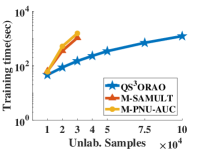
(a) 3D

(b) Sgemm

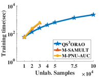
(c) Year

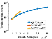
(d) Yolanda

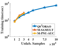
(e) Baby

(f) Beauty

(g) Clothes

(h) Pet

Figure 1: The training time of QS³ORAO, M-SAMULT and M-PNU-AUC against different sizes of unlabeled samples, where the sizes of labeled samples are fixed at 500. (The lines of M-SAMULT and M-PNU-AUC are incomplete because their implementations crash on larger training sets.)

​​​​​​​​​​​

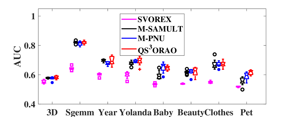
Figure 2: The boxplot of AUC results on unlabeled datasets for SVOREX, M-PNU-AUC, M-SAMULT and our QS³ORAO.

Experimental Setup

We compare the AUC results and running time of Q³ORAO with other methods summarized as follows,

1. SVOREX: Supervised OR algorithm proposed in (?).

2. M-PNU-AUC: Multi class version of PNU-AUC (?), which focuses on binary semi-supervised AUC optimization.

3. M-SAMULT: Multi class version of SAMULT (?), which focuses on binary semi-supervised AUC optimization.

We implemented QSG-ORS²AO, SVOREX and SAMULT in MATLAB. We used the MATLAB code from https://github.com/t-sakai-kure/PNU as the implementation of PNU-AUC. Originally, both PNU-AUC and SAMULT focus on binary semi-supervised AUC optimization problems. We extend them to multi-class version by using a multiclass training paradigm. Specifically, similar to our binary decomposition in our method, we use PNU-AUC and SAMUlT to training $k-1$ classifiers, $f_{j}(x)$, $j=1,\cdots,k-1$, Then we calculate the average AUC of unlabeled by Equation (2). We denote these multiclass versions as M-PNU-AUC and M-SAMULT. For all algorithms, we use the squared pairwise loss function $l(u,v)=(1-u+v)^{2}$ and Gaussian kernel $k(x,x^{\prime})=\exp(\sigma\parallel x-x^{\prime}\parallel^{2})$. The hyper-parameters ($\lambda$ and $\sigma$) were chosen via 5-fold cross-validation from the region $\{(\lambda,\gamma)|2^{-3}\leq\lambda\leq 2^{3},2^{-3}\sigma\leq 2^{3}\}$. The trade-off parameters $\{\gamma^{j}\}$ for $k-1$ subproblems were searched from $0$ to $1$ at intervals of $0.1$.

Note all the experiments were run on a PC with 56 2.2GHz cores and 80GB RAM and all the results are the average of $10$ trials.

Datasets

Table 2 summarizes $4$ regression datasets collected from UCI, LIBSVM repositories and $4$ real-world datasets from Amazon product datasets. We discretize the regression datasets into equal-frequency bins. For real-world datasets, we first use TF-IDF to process text data, and then reduce the data dimensions to $1000$ by using SVD. To conduct the experiments for semi-supervised problems, we randomly sample 500 labeled instances and drop labels of the rest instances. All the data features are normalized to $[0,1]$ in advance.

Results and Disscussion

Figure 2 presents the AUC results on the unlabeled dataset of these algorithms. The results show that in most cases, our proposed QS³ORAO has the highest AUC results. In addition, we also compare the AUC results with supervised method SVOREX which uses 500 labeled instances to train a model. Obviously, our semi-supervised learning method has higher AUC than SVOREX, which demonstrate that incorporating unlabeled instances can improve the performance.

Figure 1 presents the training time against different size of unlabeled samples. The two lines of M-SAMULT and M-PNU-AUC are incomplete. This is because these two methods need to save the whole kernel matrix, and as unlabeled data continues to increase, they are all out of memory. In contrast, QS³ORAO only need to keep $m$ random features in each iteration. This low memory requirement allows it to do an efficient training for large scale datasets. Besides, we can easily find that our method is faster than M-SAMULT and M-PNU-AUC when the number of unlabeled instances is larger than $10000$. This is because the M-SAMULT and M-PNU-AUC need $O(n^{3})$ operations to compute the inverse of kernel matrix. Differently, QS³ORAO uses RFF to approximate the kernel function, and each time it only needs $O(Dn)$ operations to calculate the random features with seed $i$.

Based on these results, we conclude that QSG-S2AUC is superior to other state-of-the-art algorithms in terms of efficiency and scalability, while retaining similar generalization performance.

Conclusion

In this paper, we propose an unbiased objective function of semi-supervised OR AUC optimization and propose a novel scalable algorithm, QS³ORAO to solve it. We decompose the original problem by $k-1$ parallel hyperplanes to $k-1$ binary semi-supervised AUC optimization problems. Then we use a DSG-based method to achieve the optimal solution. Even though this optimization process contains four sources of randomness, theoretically, we prove that QS³ORAO has a convergence rate of $O(1/t)$. The experimental results on various benchmark datasets also demonstrate the superiority of the proposed QS³ORAO.

Appendix A Detailed Proof of Ordered Rule of Thresholds

Proof 1

Firstly, take $i$-th subproblem into consideration, define the threshold is $b$. We have datasets $\{x_{i}\in\mathcal{D}_{1}\cup\cdots\cup\mathcal{D}_{j}|f(x_{i})-b<0\}$ and $\{x_{i}\in\mathcal{D}_{j+1}\cup\cdots\cup\mathcal{D}_{k}|f(x_{i})-b>0\}$. Equation (15) is equivalent to

$$e_{j}(b) =\sum_{x_{i}\in\mathcal{D}_{1}\cup\cdots\cup\mathcal{D}_{j}}(b-f(x_{i}))^{2}$$

$$+\sum_{x_{i}\in\mathcal{D}_{j+1}\cup\cdots\cup\mathcal{D}_{k}}(f(x_{i})-b)^{2}$$ A

According to the strict convexity of (1), that $b^{*}$ is unique. Then we can conclude that $\textbf{b}^{*}$ is unique.

Then we prove the order between thesholds. The derivative of $e_{j}(b)$ with respect to $b_{k}$ is

$$g_{j}(b) =\dfrac{\partial e_{j}(b)}{\partial b}$$

$$=2\sum_{x_{i}\in\mathcal{D}_{1}\cup\cdots\cup\mathcal{D}_{j}}(b-f(x_{i}))$$

$$-2\sum_{x_{i}\in\mathcal{D}_{j+1}\cup\cdots\cup\mathcal{D}_{k}}(f(x_{i})-b)$$ (17)

Suppose $b_{j}^{*}\geq b_{j+1}^{*}$. We have $g_{j}(b_{j+1}^{*})<0$ since $b_{j}^{*}$ is the minimizer of $e_{j}(b)$. Besides, since $b_{j+1}^{*}$ is minimizer of $e_{j+1}(b)$, we have $g_{k+1}(b_{j+1}^{*})=0$. Thus, we have $g_{j+1}(b_{j+1}^{*})-g_{k}(b_{j+1}^{*})>0$. However, we also have

$$\quad g_{j+1}(b_{j+1}^{*})-g_{k}(b_{j+1}^{*})$$

$$=-\sum_{x_{i}\in\mathcal{D}_{j+1}}(b_{j+1}-f(x_{i}))-2\sum_{x_{i}\in\mathcal{D}_{j+1}}(f(x_{i})-b_{j+1})\leq 0.$$ (18)

So we have $b_{j}^{*}<b_{j+1}^{*}$ and similary we can get $b_{1}^{*}<\cdots<b_{k-1}^{*}$

Appendix B Detailed Proof of Convergence Rate

In this section, we give detailed proof of Lemmas 2-4 and Theorem 1.

Proof of Lemma 2

Here we give the detailed proof of lemma 2.

Proof 2

We denote $A_{i}(x)=A_{i}(x;x_{i}^{p},x_{i}^{n},x_{i}^{u},\omega_{i}):=a_{t}^{i}(\zeta_{i}(x)-\xi_{i}(x))$. According to the assumption in section 5, $A_{i}(X)$ have a bound:

$$|A_{i}(x)| \leq |a_{t}^{i}|\left(|\zeta_{i}(x)|+|\xi_{i}(x)|\right)$$

$$\leq |a_{t}^{i}|(\dfrac{1}{k-1}\sum_{j=1}^{k-1}(\gamma^{j}(l_{1}^{j}k(x_{i}^{p},x)+l_{2}^{j}k(x_{i}^{n},x))$$

$$+(1-\gamma^{j})(l_{3}^{j}k(x_{i}^{p},x)+l_{4}^{j}k(x_{i}^{u},x)$$

$$+l_{5}^{j}k(x_{i}^{u},x)+l_{6}^{j}k(x_{i}^{n},x)))$$

$$+\dfrac{1}{k-1}\sum_{j=1}^{k-1}(\gamma^{j}(l_{1}^{j}\phi_{\omega}(x^{p})\phi_{\omega}(x)+l_{2}^{j}\phi_{\omega}(x^{n})\phi_{\omega}(x)$$

$$+(1-\gamma^{j})(l_{3}^{j}\phi_{\omega}(x^{p})\phi_{\omega}(x)+l_{4}^{j}\phi_{\omega}(x^{u})\phi_{\omega}(x)$$

$$+l_{5}^{j}\phi_{\omega}(x^{u})\phi_{\omega}(x)+l_{6}^{j}\phi_{\omega}(x^{n})\phi_{\omega}(x)))))$$

$$\leq |a_{t}^{i}|(\dfrac{1}{k-1}\sum_{j=1}^{k-1}(\gamma^{j}(M_{1}+M_{2})$$

$$+(1-\gamma^{j})(M_{1}+M_{2}+M_{1}+M_{2}))\kappa$$

$$+\dfrac{1}{k-1}(\gamma^{j}(M_{1}+M_{2})$$

$$+(1-\gamma^{j})(M_{1}+M_{2}+M_{1}+M_{2}))\phi)$$

$$= M(\kappa+\phi)|a_{t}^{i}|$$

Then we obtain the lemma 2. This completes the proof.

Proof of lemma 5

Lemma 5

Suppose $\eta_{i}=\dfrac{\theta}{i}$ ($1\leq i\leq t$) and $\theta\lambda\in(1,2)\cup\mathbb{Z}_{+}$. We have $|a_{t}^{i}|\leq\dfrac{\theta}{t}$ and $\sum_{i=1}^{t}|a_{t}^{i}|^{2}\leq\dfrac{\theta^{2}}{t}$.

Proof 3

Obviously, $|a_{t}^{i}|\leq\dfrac{\theta}{t}$. Then we have

$$|a_{t}^{i}| =|a_{t}^{i+1}\dfrac{\eta_{i}}{\eta_{i+1}}(1-\lambda\eta_{i+1})|$$

$$=\dfrac{i+1}{i}|1-\dfrac{\lambda\theta}{i+1}|\cdot|a_{t}^{i+1}|$$

$$=|\dfrac{i+1-\lambda\theta}{i}|\cdot|a_{t}^{i+1}|$$

When $\lambda\theta\in(1,2),\forall i\geq 1$, we have $i-1<i+1-\lambda\theta<i$, so $|a_{t}^{i}|<|a_{t}^{i+1}|\leq\dfrac{\theta}{t}$ and $\sum_{i=1}^{t}\leq\dfrac{\theta^{2}}{t}$. When $\lambda\theta\in\mathbb{Z}_{+}$, if $i>\lambda\theta-1$, then $|a_{t}^{i}|<|a_{t}^{i+1}|\leq\dfrac{\theta}{t}$. If $i\leq\lambda\theta-1$, then $|a_{t}^{i}|=0$. So we get $\sum_{i=1}^{t}|a_{t}^{i}|^{2}\leq\dfrac{\theta^{2}}{t}$. Therefore, we obtain the lemma 5. This completes the proof.

Proof of Lemma 4

In $j$-th subproblem, we denote that $l_{1}^{\prime}(h(x_{t}^{p}),h(x_{t}^{n}))$, $l_{2}^{\prime}(h(x_{t}^{p}),h(x_{t}^{n}))$, $l_{1}^{\prime}(h(x_{t}^{p}),h(x_{t}^{u}))$, $l_{2}^{\prime}(h(x_{t}^{p}),h(x_{t}^{u}))$, $l_{1}^{\prime}(h(x_{t}^{u}),h(x_{t}^{n}))$ and $l_{2}^{\prime}(h(x_{t}^{u}),h(x_{t}^{n}))$ as $\tilde{l}_{1}^{j}$, $\tilde{l}_{2}^{j}$, $\tilde{l}_{3}^{j}$, $\tilde{l}_{4}^{j}$, $\tilde{l}_{5}^{j}$ and $\tilde{l}_{6}^{j}$, respectively. In addition,

We define the following three different gradient terms,

$$g_{t} = \xi_{t}+\lambda h_{t}$$

$$= \dfrac{1}{k-1}\sum_{j=1}^{k-1}(\gamma^{j}(l_{1}^{j}k(x_{t}^{p},\cdot)+l_{2}^{j}k(x_{t}^{n},\cdot))$$

$$+(1-\gamma^{j})(l_{3}^{j}k(x_{t}^{p},\cdot)+l_{4}^{j}k(x_{t}^{u},\cdot)$$

$$+l_{5}^{j}k(x_{t}^{u},\cdot)+l_{6}^{j}k(x_{t}^{n},\cdot)))+\lambda h_{t}$$

$$\hat{g_{t}} = \hat{\xi_{t}}+\lambda h_{t}$$

$$= \dfrac{1}{k-1}\sum_{j=1}^{k-1}(\gamma^{j}(\tilde{l}_{1}^{j}k(x_{t}^{p},\cdot)+\tilde{l}_{2}^{j}k(x_{t}^{n},\cdot))$$

$$+(1-\gamma^{j})(\tilde{l}_{3}^{j}k(x_{t}^{p},\cdot)+\tilde{l}_{4}^{j}k(x_{t}^{u},\cdot)$$

$$+\tilde{l}_{5}^{j}k(x_{t}^{u},\cdot)+\tilde{l}_{6}^{j}k(x_{t}^{n},\cdot)))+\lambda h_{t}$$

$$\bar{g_{t}} = \mathbb{E}_{x_{t}^{p},x_{t}^{n},x_{t}^{u}}[\hat{g_{t}}]$$

$$= \mathbb{E}_{x_{t}^{p},x_{t}^{n}x_{t}^{u}}[\dfrac{1}{k-1}\sum_{j=1}^{k-1}(\gamma(\tilde{l}_{1}^{j}k(x_{t}^{p},\cdot)+\tilde{l}_{2}^{j}k(x_{t}^{n},\cdot))$$

$$+(1-\gamma)(\tilde{l}_{3}^{j}k(x_{t}^{p},\cdot)+\tilde{l}_{4}^{j}k(x_{t}^{u},\cdot)$$

$$+\tilde{l}_{5}^{j}k(x_{t}^{u},\cdot)+\tilde{l}_{6}^{j}k(x_{t}^{n},\cdot)))]+\lambda h_{t}$$

Note that from our previous definition, we have $h_{t+1}=h_{t}-\eta_{t}g_{t},\forall t\geq 1$.

Denote $A_{t}=\parallel h_{t}-f^{*}\parallel_{\mathcal{H}}^{2}$. Then we have

$$A_{t+1} = \parallel h_{t}-f^{*}-\eta_{t}g_{t}\parallel_{\mathcal{H}}^{2}$$

$$= A_{t}+\eta_{t}^{2}\parallel g_{t}\parallel_{\mathcal{H}}^{2}-2\eta_{t}\langle h_{t}-f^{*},g_{t}\rangle_{\mathcal{H}}$$

$$= A_{t}+\eta_{t}^{2}\parallel g_{t}\parallel_{\mathcal{H}}^{2}-2\eta_{t}\langle h_{t}-f^{*},\bar{g_{t}}\rangle_{\mathcal{H}}$$

$$+2\eta_{t}\langle h_{t}-f^{*},\bar{g_{t}}-\hat{g_{t}}\rangle_{\mathcal{H}}+2\eta_{t}\langle h_{t}-f^{*},\hat{g_{t}}-g_{t}\rangle_{\mathcal{H}}$$

Because of the strongly convexity of loss function and optimality condition, we have

$$\langle h_{t}-f^{*},\bar{g_{t}}\rangle_{\mathcal{H}}\geq\lambda\parallel h_{t}-f^{*}\parallel_{\mathcal{H}}^{2}$$

Hence, we have

$$A_{t+1} \leq(1-2\eta_{t}\lambda)A_{t}+\eta_{t}^{2}\parallel g_{t}\parallel_{\mathcal{H}}^{2}+2\eta_{t}\langle h_{t}-f^{*},\bar{g_{t}}-\hat{g_{t}}\rangle_{\mathcal{H}}$$

$$\quad+2\eta_{t}\langle h_{t}-f^{*},\hat{g_{t}}-g_{t}\rangle_{\mathcal{H}},\forall t\geq 1$$ (19)

Let us denote $\mathcal{M}_{t}=\parallel g_{t}\parallel_{\mathcal{H}}^{2}$, $\mathcal{N}_{t}=\langle h_{t}-f^{*},\bar{g_{t}}-\hat{g_{t}}\rangle_{\mathcal{H}}$, $\mathcal{R}_{t}=\langle h_{t}-f^{*},\hat{g_{t}}-g_{t}\rangle_{\mathcal{H}}$. Firstly, we show that $\mathcal{M}_{t}$, $\mathcal{N}_{t}$, $\mathcal{R}_{t}$ are bounded. Specifically, for $t\geq 1$, we have

$$\mathcal{M}_{t}\leq\kappa M^{2}(1+\lambda c_{t})$$ (20)

where $c_{t}:=\sqrt{\sum_{i,j=1}^{t-1}|a_{t-1}^{i}||a_{t-1}^{j}|}$

$$\mathbb{E}_{x_{t}^{p},x_{t}^{n},x_{t}^{u},\omega_{t}}[\mathcal{N}_{t}]=0$$ (21)

$$\mathbb{E}_{x_{t}^{p},x_{t}^{n}x_{t}^{u},\omega_{t}}[\mathcal{R}_{t}]\leq\kappa^{1/2}LB_{1,t}\sqrt{\mathbb{E}_{x_{t-1}^{p},x_{t-1}^{n},x_{t-1}^{u},\omega_{t-1}}[A_{t}]}$$ (22)

where $M:=\dfrac{1}{k-1}\sum_{j=1}^{k-1}(2-\gamma^{j})(M_{1}+M_{2})$, $L:=\dfrac{1}{k-1}\sum_{j=1}^{k-1}(2-\gamma^{j})(L_{1}+L_{2})$ and $A_{t}=\parallel h_{t}-f^{*}\parallel_{\mathcal{H}}^{2}$.

Proof 4

The proof of Eq. (20):

$$\mathcal{M}_{t}=\parallel g_{t}\parallel_{\mathcal{H}}^{2}=\parallel\xi_{t}+\lambda h_{t}\parallel_{\mathcal{H}}^{2}\leq\left(\parallel\xi\parallel_{\mathcal{H}}+\lambda\parallel h_{t}\parallel_{\mathcal{H}}\right)^{2}$$

and

$$\parallel\xi_{t}\parallel_{\mathcal{H}} = \parallel\dfrac{1}{k-1}\sum_{j=1}^{k-1}(\gamma^{j}(l_{1}^{j}k(x_{t}^{p},\cdot)+l_{2}^{j}k(x_{t}^{n},\cdot))$$

$$+(1-\gamma^{j})(l_{3}^{j}k(x_{t}^{p},\cdot)+l_{4}^{j}k(x_{t}^{u},\cdot)$$

$$+l_{5}^{j}k(x_{t}^{u},\cdot)+l_{6}^{j}k(x_{t}^{n},\cdot)))\parallel_{\mathcal{H}}$$

$$\leq \kappa^{1/2}(\dfrac{1}{k-1}\sum_{j=1}^{k-1}(\gamma^{j}(M_{1}+M_{2})$$

$$+(1-\gamma^{j})(M_{1}+M_{2}+M_{1}+M_{2})))$$

$$= \kappa^{1/2}M$$

Then we have:

$$\|h_{t}\|_{\mathcal{H}}^{2} = \sum_{i=1}^{t-1}\sum_{j=1}^{t-1}a_{t-1}^{i}a_{t-1}^{j}\dfrac{1}{k-1}\sum_{j=1}^{k-1}[\gamma^{j}(l_{1}^{j}k(x_{i}^{p},\cdot)+l_{2}^{j}k(x_{i}^{n},\cdot))$$

$$+(1-\gamma^{j})(l_{3}^{j}k(x_{i}^{p},\cdot)+l_{4}^{j}k(x_{i}^{u},\cdot)$$

$$+l_{5}^{j}k(x_{i}^{u},\cdot)+l_{6}^{j}k(x_{i}^{n},\cdot))]$$

$$\cdot\dfrac{1}{k-1}\sum_{j=1}^{k-1}[\gamma^{j}(l_{1}^{j}k(x_{j}^{p},\cdot)+l_{2}^{j}k(x_{j}^{n},\cdot))$$

$$+(1-\gamma^{j})(l_{3}^{j}k(x_{j}^{p},\cdot)+l_{4}^{j}k(x_{j}^{u},\cdot)$$

$$+l_{5}^{j}k(x_{j}^{u},\cdot)+l_{6}^{j}k(x_{j}^{n},\cdot))]$$

$$\leq \kappa\dfrac{1}{(k-1)^{2}}\sum_{n,m}^{k-1}\sum_{i=1}^{t-1}\sum_{j=1}^{t-1}a_{t-1}^{i}a_{t-1}^{j}[\gamma^{j}\gamma^{j}(M_{1}+M_{2})^{2}$$

$$+2\gamma^{j}(1-\gamma^{j})(M_{1}+M_{2})(M_{1}+M_{2}+M_{1}+M_{2})$$

$$+(1-\gamma^{j})^{2}(M_{1}+M_{2}+M_{1}+M_{2})^{2}]$$

$$= \kappa\sum_{i=1}^{t-1}\sum_{j=1}^{t-1}a_{t-1}^{i}a_{t-1}^{j}[\dfrac{1}{k-1}\sum_{j=1}^{k-1}(2-\gamma^{j})(M_{1}+M_{2})]^{2}$$

$$= \kappa M^{2}\sum_{i=1}^{t-1}\sum_{j=1}^{t-1}a_{t-1}^{i}a_{t-1}^{j}$$

Then we obtain Eq. (20).

Proof 5

The proof of Eq. (21)

$$\mathbb{E}_{x_{t}^{p},x_{t}^{n},x_{t}^{u},\omega_{t}}[\mathcal{N}_{t}]$$

$$= \mathbb{E}_{x_{t-1}^{p},x_{t-1}^{n},x_{t-1}^{u},\omega_{t}}$$

$$\left[\mathbb{E}_{x_{t}^{p},x_{t}^{n},x_{t}^{u}}[\langle h_{t}-f^{*},\bar{g_{t}}-\hat{g_{t}}\rangle_{\mathcal{H}}|x_{t-1}^{p},x_{t-1}^{u},\omega_{t}]\right]$$

$$= \mathbb{E}_{x_{t-1}^{p},x_{t-1}^{n},x_{t-1}^{u},\omega_{t}}\left[\langle h_{t}-f^{*},\mathbb{E}_{x_{t-1}^{p},x_{t-1}^{n},x_{t-1}^{u}}[\bar{g_{t}}-\hat{g_{t}}]\rangle_{\mathcal{H}}\right]$$

$$= 0$$

Proof 6

The proof of Eq. (22)

$$\mathbb{E}_{x_{t}^{p},x_{t}^{n},x_{t}^{u},\omega_{t}}[\mathcal{R}_{t}]$$

$$= \mathbb{E}_{x_{t}^{p},x_{t}^{n},x_{t}^{u},\omega_{t}}[\langle h_{t}-f^{*},\hat{g_{t}}-g_{t}\rangle_{\mathcal{H}}]$$

$$= \mathbb{E}_{x_{t}^{p},x_{t}^{n},x_{t}^{u},\omega_{t}}[\langle h_{t}-f^{*},\dfrac{1}{k-1}\sum_{j=1}^{k-1}\gamma^{j}[(l_{1}^{j}-\tilde{l}_{1}^{j})k(x_{t}^{p},\cdot)$$

$$+(l_{2}^{j}-\tilde{l}_{2}^{j})k(x_{t}^{n},\cdot)]$$

$$+(1-\gamma^{j})[(l_{3}^{j}-\tilde{l}_{3}^{j})k(x_{t}^{p},\cdot)+(l_{4}^{j}-\tilde{l}_{4}^{j})k(x_{t}^{u},\cdot)$$

$$+(l_{5}^{j}-\tilde{l}_{5}^{j})k(x_{t}^{u},\cdot)+(l_{6}^{j}-\tilde{l}_{6}^{j})k(x_{t}^{n},\cdot)]\rangle_{\mathcal{H}}]$$

$$\leq \mathbb{E}_{x_{t}^{p},x_{t}^{p},x_{t}^{u},\omega_{t}}[\parallel h_{t}-f^{*}\parallel_{\mathcal{H}}$$

$$\cdot\dfrac{1}{k-1}\sum_{j=1}^{k-1}\gamma^{j}[|l_{1}^{j}-\tilde{l}_{1}^{j}|\cdot\parallel k(x_{t}^{p},\cdot)\parallel_{\mathcal{H}}$$

$$+|l_{2}^{j}-\tilde{l}_{2}^{j}|\parallel k(x_{t}^{n},\cdot)\parallel_{\mathcal{H}}]$$

$$+(1-\gamma^{j})[|l_{3}^{j}-\tilde{l}_{3}^{j}|\parallel k(x_{t}^{p},\cdot)\parallel_{\mathcal{H}}+|l_{4}^{j}-\tilde{l}_{4}^{j}|\parallel k(x_{t}^{u},\cdot)\parallel_{\mathcal{H}}$$

$$+|l_{5}^{j}-\tilde{l}_{5}^{j}|\parallel k(x_{t}^{u},\cdot)\parallel_{\mathcal{H}}+|l_{6}^{j}-\tilde{l}_{6}^{j}|\parallel k(x_{t}^{n},\cdot)\parallel_{\mathcal{H}}]]$$

$$\leq \kappa^{1/2}\mathbb{E}_{x_{t}^{p},x_{t}^{u},x_{t}^{u},\omega_{t}}[\parallel h_{t}-f^{*}\parallel_{\mathcal{H}}$$

$$\cdot\dfrac{1}{k-1}\sum_{j=1}^{k-1}[\gamma^{j}(|l_{1}^{j}-\tilde{l}_{1}^{j}|+|l_{2}^{j}-\tilde{l}_{2}^{j}|)$$

$$+(1-\gamma^{j})(|l_{3}^{j}-\tilde{l}_{3}^{j}|+|l_{4}^{j}-\tilde{l}_{4}^{j}|+|l_{5}^{j}-\tilde{l}_{5}^{j}|+|l_{6}^{j}-\tilde{l}_{6}^{j}|)]]$$

$$\leq \kappa^{1/2}\mathbb{E}_{x_{t}^{p},x_{t}^{n},x_{t}^{u},\omega_{t}}[\|h_{t}-f^{*}\|_{\mathcal{H}}$$

$$\cdot\dfrac{1}{k-1}\sum_{j=1}^{k-1}[\gamma^{j}(L_{1}|f_{t}(x_{t}^{p})-h_{t}(x_{t}^{p})|$$

$$+L_{2}|f_{t}(x_{t}^{n})-h_{t}(x_{t}^{n})|)$$

$$+(1-\gamma^{j})(L_{1}|f_{t}(x_{t}^{p})-h_{t}(x_{t}^{p})|+L_{2}|f_{t}(x_{t}^{u})-h_{t}(x_{t}^{u})|$$

$$+L_{1}|f_{t}(x_{t}^{u})-h_{t}(x_{t}^{u})|+L_{2}|f_{t}(x_{t}^{n})-h_{t}(x_{t}^{n})|)]]$$

$$\leq \kappa^{1/2}\sqrt{\mathbb{E}_{x_{t}^{p},x_{t}^{n},x_{t}^{u},\omega_{t}}[A_{t}]}$$

$$\cdot\sqrt{[\dfrac{1}{k-1}\sum_{j=1}^{k-1}(2-\gamma^{j})(L_{1}+L_{2})]^{2}B_{1,t}^{2}}$$

$$\leq \kappa^{1/2}LB_{1,t}\sqrt{\mathbb{E}_{x_{t-1}^{p},x_{t-1}^{n},x_{t-1}^{u},\omega_{t-1}}[A_{t}]}$$

The first and third inequalities are due to Cauchy-Schwarz Inequality and the second inequality is due to the Assumption 3. And the last step is due to the Lemma 2 and the definition of $A_{t}$.

After proving the Eq. (20)-(22) separately, let us denote $e_{t}=\mathbb{E}_{x_{t}^{p},x_{t}^{u},\omega_{t}}[A_{t}]$, given the above bounds, we arrive the following recursion,

$$e_{t+1}\leq(1-2\eta_{t}\lambda)e_{t}+\kappa M^{2}\eta_{t}^{2}(1+\lambda c_{t})^{2}+2\kappa^{1/2}L\eta_{t}B_{1,t}\sqrt{e_{t}}$$

When $\eta_{t}=\dfrac{\theta}{t}$ with $\theta$ such that $\theta\lambda\in(1,2)\cup\mathbb{Z}_{+}$, from Lemma 5, we have $|a_{t}^{i}|\leq\dfrac{\theta}{t}$, $\forall 1\leq i\leq t$. Consequently, $c_{t}\leq\theta$ and $B_{1,t}^{2}\leq M^{2}(\kappa+\phi)^{2}\dfrac{\theta^{2}}{t-1}$. Applying these bounds to the above recursion, we have $e_{t+1}\leq(1-\dfrac{2\theta\lambda}{t})e_{t}+\kappa^{2}\dfrac{\theta^{2}}{t^{2}}(1+\lambda\theta)^{2}+2\kappa^{1/2}\dfrac{\theta}{t}L\eta_{t}\sqrt{M^{2}(\kappa+\phi)^{2}\dfrac{\theta^{2}}{t-1}}\sqrt{e_{t}}$ and then it can be rewritten as:

$$e_{t+1}\leq(1-\dfrac{2\theta\lambda}{t})e_{t}+\dfrac{\beta_{1}}{t}\sqrt{\dfrac{e_{t}}{t}}+\dfrac{\beta_{2}}{t^{2}}$$

where $\beta_{1}=2\sqrt{2}\kappa^{1/2}LM(\kappa+\phi)\theta^{2}$ ($\sqrt{\dfrac{t}{t-q}}\leq\sqrt{2}$) and $\beta_{2}=\kappa M^{2}\theta^{2}(1+\lambda\theta)^{2}$. Reusing Lemma 14 in [Dai et al., 2014] with $\eta=2\theta\lambda>1$ leads to

$$e_{t+1}\leq\dfrac{Q_{1}^{2}}{t}$$

where

$$Q_{1}=\max\left\{\parallel f^{*}\parallel_{\mathcal{H}},\dfrac{Q_{0}+\sqrt{Q_{0}^{2}+(2\theta\lambda-1)(1+\theta\lambda)^{2}\theta^{2}\kappa M^{2}}}{2\theta\lambda-1}\right\}$$

and $Q_{0}=2\sqrt{2}\kappa^{1/2}(\kappa+\phi)LM\theta^{2}$.

Proof of Theorem 1

Proof 7

Substitute Lemma 2 and 4 into Eq. (16), we have that

$$\mathbb{E}_{x_{t}^{p},x_{t}^{u},\omega_{t}}[|f_{t}(x)-f^{*}(x)|^{2}] \leq 2\mathbb{E}_{x_{t}^{p},x_{t}^{u},\omega_{t}}[|f_{t}(x)-h_{t+1}(x)|^{2}]$$

$$+2\kappa\mathbb{E}_{x_{t}^{p},x_{t}^{u},\omega_{t}}[\parallel h_{t}-f^{*}\parallel_{\mathcal{H}}]$$

$$\leq 2B_{1,t+1}^{2}+2\kappa\dfrac{Q_{1}^{2}}{t}$$

$$\leq \dfrac{2C^{2}+2\kappa Q_{1}^{2}}{t}$$

where the last inequality is due to Lemma 5. In this way, we obtain the final result on convergence in expectation. This completes the proof.

References

• [Belkin, Niyogi, and Sindhwani 2006] Belkin, M.; Niyogi, P.; and Sindhwani, V. 2006. Manifold regularization: A geometric framework for learning from labeled and unlabeled examples. Journal of machine learning research 7(Nov):2399–2434.
• [Chapelle, Scholkopf, and Zien 2009] Chapelle, O.; Scholkopf, B.; and Zien, A. 2009. Semi-supervised learning. IEEE Transactions on Neural Networks 20(3):542–542.
• [Chu and Keerthi 2007] Chu, W., and Keerthi, S. S. 2007. Support vector ordinal regression. Neural computation 19(3):792–815.
• [Dai et al. 2014] Dai, B.; Xie, B.; He, N.; Liang, Y.; Raj, A.; Balcan, M.-F. F.; and Song, L. 2014. Scalable kernel methods via doubly stochastic gradients. In Advances in NIPS, 3041–3049.
• [Drineas and Mahoney 2005] Drineas, P., and Mahoney, M. W. 2005. On the nyström method for approximating a gram matrix for improved kernel-based learning. journal of machine learning research 6(Dec):2153–2175.
• [Fathony, Bashiri, and Ziebart 2017] Fathony, R.; Bashiri, M. A.; and Ziebart, B. 2017. Adversarial surrogate losses for ordinal regression. In Advances in NIPS, 563–573.
• [Fine and Scheinberg 2001] Fine, S., and Scheinberg, K. 2001. Efficient svm training using low-rank kernel representations. Journal of Machine Learning Research 2(Dec):243–264.
• [Fujino and Ueda 2016] Fujino, A., and Ueda, N. 2016. A semi-supervised auc optimization method with generative models. In ICDM, 883–888.
• [Fullerton and Xu 2012] Fullerton, A. S., and Xu, J. 2012. The proportional odds with partial proportionality constraints model for ordinal response variables. Social science research 41(1):182–198.
• [Fürnkranz, Hüllermeier, and Vanderlooy 2009] Fürnkranz, J.; Hüllermeier, E.; and Vanderlooy, S. 2009. Binary decomposition methods for multipartite ranking. In Joint European Conference on Machine Learning and Knowledge Discovery in Databases, 359–374. Springer.
• [Gao and Zhou 2015] Gao, W., and Zhou, Z.-H. 2015. On the consistency of auc pairwise optimization. In IJCAI, 939–945.
• [Gao et al. 2013] Gao, W.; Jin, R.; Zhu, S.; and Zhou, Z.-H. 2013. One-pass auc optimization. In International Conference on Machine Learning, 906–914.
• [Geng et al. 2019] Geng, X.; Gu, B.; Li, X.; Shi, W.; Zheng, G.; and Huang, H. 2019. Scalable semi-supervised svm via triply stochastic gradients. In IJCAI.
• [Gu et al. 2015] Gu, B.; Sheng, V. S.; Tay, K.; Romano, W.; and Li, S. 2015. Incremental support vector learning for ordinal regression. IEEE Transactions on Neural Networks and Learning Systems 26:1403–1416.
• [Gu et al. 2018a] Gu, B.; Shan, Y.; Geng, X.; and Zheng, G. 2018a. Accelerated asynchronous greedy coordinate descent algorithm for svms. In IJCAI, 2170–2176.
• [Gu et al. 2018b] Gu, B.; Xin, M.; Huo, Z.; and Huang, H. 2018b. Asynchronous doubly stochastic sparse kernel learning. In Thirty-Second AAAI Conference on Artificial Intelligence.
• [Gu, Huo, and Huang 2019] Gu, B.; Huo, Z.; and Huang, H. 2019. Scalable and efficient pairwise learning to achieve statistical accuracy. In Proceedings of the AAAI Conference on Artificial Intelligence, volume 33, 3697–3704.
• [Gu, Xian, and Huang 2019] Gu, B.; Xian, W.; and Huang, H. 2019. Asynchronous stochastic frank-wolfe algorithms for non-convex optimization. IJCAI-19.
• [Gu 2018] Gu, B. 2018. A regularization path algorithm for support vector ordinal regression. Neural Networks 98:114–121.
• [Han et al. 2018] Han, B.; Yao, Q.; Yu, X.; Niu, G.; Xu, M.; Hu, W.; Tsang, I.; and Sugiyama, M. 2018. Co-teaching: Robust training of deep neural networks with extremely noisy labels. In Advances in NIPS, 8527–8537.
• [Kim and Ahn 2012] Kim, K.-j., and Ahn, H. 2012. A corporate credit rating model using multi-class support vector machines with an ordinal pairwise partitioning approach. Computers & Operations Research 39(8):1800–1811.
• [Li et al. 2017] Li, X.; Gu, B.; Ao, S.; Wang, H.; and Ling, C. X. 2017. Triply stochastic gradients on multiple kernel learning. In UAI.
• [Liu et al. 2011] Liu, Y.; Liu, Y.; Zhong, S.; and Chan, K. C. 2011. Semi-supervised manifold ordinal regression for image ranking. In Proceedings of the 19th ACM international conference on Multimedia, 1393–1396. ACM.
• [Niu et al. 2016] Niu, Z.; Zhou, M.; Wang, L.; Gao, X.; and Hua, G. 2016. Ordinal regression with multiple output cnn for age estimation. In Proceedings of the CVPR, 4920–4928.
• [Rahimi and Recht 2008] Rahimi, A., and Recht, B. 2008. Random features for large-scale kernel machines. In Advances in NIPS, 1177–1184.
• [Rudin 2017] Rudin, W. 2017. Fourier analysis on groups. Courier Dover Publications.
• [Sakai, Niu, and Sugiyama 2018] Sakai, T.; Niu, G.; and Sugiyama, M. 2018. Semi-supervised auc optimization based on positive-unlabeled learning. Machine Learning 107(4):767–794.
• [Seah, Tsang, and Ong 2012] Seah, C.-W.; Tsang, I. W.; and Ong, Y.-S. 2012. Transductive ordinal regression. IEEE transactions on neural networks and learning systems 23(7):1074–1086.
• [Shi et al. 2019] Shi, W.; Gu, B.; Li, X.; Geng, X.; and Huang, H. 2019. Quadruply stochastic gradients for large scale nonlinear semi-supervised auc optimization. In IJCAI.
• [Smola and Schölkopf 2000] Smola, A. J., and Schölkopf, B. 2000. Sparse greedy matrix approximation for machine learning.
• [Srijith, Shevade, and Sundararajan 2013] Srijith, P.; Shevade, S.; and Sundararajan, S. 2013. Semi-supervised gaussian process ordinal regression. In Joint European conference on machine learning and knowledge discovery in databases, 144–159. Springer.
• [Tsuchiya et al. 2019] Tsuchiya, T.; Charoenphakdee, N.; Sato, I.; and Sugiyama, M. 2019. Semi-supervised ordinal regression based on empirical risk minimization. CoRR abs/1901.11351.
• [Uematsu and Lee 2014] Uematsu, K., and Lee, Y. 2014. Statistical optimality in multipartite ranking and ordinal regression. IEEE transactions on pattern analysis and machine intelligence 37(5):1080–1094.
• [Waegeman and De Baets 2010] Waegeman, W., and De Baets, B. 2010. A survey on roc-based ordinal regression. In Preference learning. Springer. 127–154.
• [Waegeman, De Baets, and Boullart 2008] Waegeman, W.; De Baets, B.; and Boullart, L. 2008. Roc analysis in ordinal regression learning. Pattern Recognition Letters 29(1):1–9.
• [Wang et al. 2015] Wang, S.; Li, D.; Petrick, N.; Sahiner, B.; Linguraru, M. G.; and Summers, R. M. 2015. Optimizing area under the roc curve using semi-supervised learning. Pattern recognition 48(1):276–287.
• [Xie and Li 2018] Xie, Z., and Li, M. 2018. Semi-supervised auc optimization without guessing labels of unlabeled data.
• [Yan 2014] Yan, H. 2014. Cost-sensitive ordinal regression for fully automatic facial beauty assessment. Neurocomputing 129:334–342.
• [Yu et al. 2019] Yu, S.; Gu, B.; Ning, K.; Chen, H.; Pei, J.; and Huang, H. 2019. Tackle balancing constraint for incremental semi-supervised support vector learning. In Proceedings of the 25th ACM SIGKDD International Conference on Knowledge Discovery & Data Mining, 1587–1595. ACM.
• [Zhang et al. 2019] Zhang, C.; Ren, D.; Liu, T.; Yang, J.; and Gong, C. 2019. Positive and unlabeled learning with label disambiguation. In Proceedings of IJCAI-19, 4250–4256.